

Submitted:
12 October 2026
Posted:
13 October 2026
You are already at the latest version
Abstract
Credit-risk models may become unreliable when longitudinal observations are incomplete and predictive uncertainty is ignored. We propose a Structured Dynamic Bayesian Network and Bayesian Neural Network (Structured DBN + BNN) combining borrower-conditioned latent-state transitions, differentiable filtering, complementary GRU and direct-input encoders, and variational Bayesian discrimination. Training-time masking improves robustness to missing evidence, while reconstruction regularizes the latent states. At inference, Monte Carlo sampling, validation-based temperature scaling, predictive entropy, and mutual information support calibrated prediction and uncertainty-aware triage. On the Default of Credit Card Clients dataset, ten paired seeded evaluations show competitive clean-data discrimination, with an AUROC of 0.7828. Under 30% MCAR missingness, the model achieves an AUROC of 0.7623 and achieves a higher mean AUROC than the principal baselines drawn from recurrent, Bayesian, and Transformer model families; similar robustness is observed under MAR, MNAR, and recent-month removal. At 10% selective coverage, entropy-based ranking reduces the mean error to 3.51%. These findings show that the framework’s main benefit is robust, uncertainty-aware prediction when temporal evidence is incomplete, rather than uniformly superior discrimination on complete data.
Keywords:
credit risk prediction
; dynamic Bayesian network
; Bayesian neural network
; uncertainty quantification
; missing data
1. Introduction
Credit scoring maps borrower information to default risk, supporting approval and monitoring decisions [1]. Machine-learning methods offer nonlinear discrimination [2], while recent reviews highlight diverse representations and learning strategies [3]. Yet credit histories are longitudinal: repayment status, bill amounts, and payments evolve, while recent observations may be delayed or missing. Robustness to incomplete temporal evidence is important [4]. Existing methods address this only partially. Flattened models ignore state evolution, whereas recurrent networks lack structured transitions. Dynamic Bayesian networks provide latent-state filtering [5], and variational Bayesian neural networks capture weight-related epistemic uncertainty through posterior predictive averaging [6]. Credit-risk research has begun to quantify predictive uncertainty [7], but calibration remains essential because discrimination alone does not ensure reliable probabilities [8]. Practical models should combine temporal structure, missing-data robustness, calibration, and uncertainty-aware triage.
Related studies in financial machine learning and probabilistic modeling address complementary issues. Hidden-state modeling has been used to characterize heterogeneous firm trajectories under incomplete market signals [9]. Structured inference networks learn nonlinear state-space models through recurrent variational approximations [10]. Additive feature attribution supports individual prediction explanations [11], while sparse-dense representations have been studied in financial document retrieval [12]. In fraud detection, classifiers trained on investigator feedback and delayed labels address distinct sources of supervision [13]. Transformer-based methods have also been used to represent temporal and relational patterns in financial transactions [14]. Example-dependent cost-sensitive trees incorporate financial losses into decision rules [15]. Bayesian conditional density estimation supports likelihood-free posterior inference [16]. Zhang et al. propose kernel-adaptive synthetic posterior estimation (KASPE), which learns posterior representations from simulated datasets without explicit likelihood evaluations [17]. Zhu and Zhang introduce AIM, an amortized Bayesian inference framework for multistate transition models that supports efficient posterior estimation and uncertainty quantification [18]. Financial named-entity recognition research has separately examined confidence under domain shift [19]. These methods provide context for Bayesian inference and temporal state modeling, but do not directly establish robustness for longitudinal credit-default prediction.
Recent credit-risk studies further illustrate several closely related methodological directions. Regarding temporal modeling, recurrent neural networks have been applied to retail customers’ credit histories [20], while Transformer architectures have been used to predict multi-horizon corporate default from longitudinal observations [21]. Regarding incomplete credit information, GAN-based multiple imputation has been proposed to reconstruct missing credit-risk data [22]. Regarding uncertainty-aware decision making, profit and risk have been evaluated under uncertain cost parameters [23], three-way decision models have been used to identify uncertain cases among Chinese SMEs [24], and profit-based uncertainty measures have been incorporated into credit-scoring systems with a rejection option [25]. These studies demonstrate the importance of temporal representations, missing-data handling, and uncertainty-aware decisions. However, these issues are generally addressed separately, leaving a need for an integrated framework that models borrower-specific temporal dynamics while maintaining robust and calibrated predictions when monthly evidence is incomplete.
We propose a Structured DBN + BNN for default prediction using static attributes and six monthly observations. Static features determine initial latent states and borrower-specific transitions, while differentiable Bayesian filtering incorporates monthly evidence. Trajectory summaries are fused with GRU and direct-input MLP representations and classified by a variational Bayesian discriminator. Training uses masking for robustness to missing data, auxiliary reconstruction for regularization, and validation-only temperature scaling to calibrate predictions.
Our contributions are: (1) structured borrower-specific temporal evolution; (2) fusion of filtering, observation-level encoders, and Bayesian uncertainty; and (3) ten-seed comparisons with tree, recurrent, static-Bayesian, and Transformer–MC-dropout baselines under MCAR, recent-block, MAR, and MNAR missingness, with sensitivity and CPU cost/scaling analyses. Sections II–IV present the method, experiments, and conclusions.
2. Method
2.1. Problem Formulation and Architecture
Let be a credit-risk dataset with customers. The static vector contains time-invariant customer attributes (e.g., demographic information and static credit history). The ordered sequence consists of monthly observations from the oldest to the most recent month; in this application , and each comprises repayment status, bill amount, and payment amount after training-set transformations. The binary label indicates whether the customer defaults in the following month.
Our goal is to predict default probability while quantifying uncertainty. Calibration is evaluated separately and, when necessary, adjusted using validation data. The architecture combines three complementary components. A static-conditioned DBN models borrower-specific temporal transitions and filters monthly evidence. Parallel GRU and direct-input MLP pathways preserve observation-level information that may be lost in the finite-state representation. A variational Bayesian discriminator captures epistemic uncertainty arising from limited data. As shown in Figure 1, static covariates determine the initial-state distribution and transition matrix, while monthly observations update the latent-state trajectory. The terminal state, trajectory summary, GRU representation, and MLP features are fused for Bayesian prediction. An auxiliary reconstruction branch regularizes the latent states during training but is removed at inference. Together, these components preserve temporal structure without forcing information through a discrete-state bottleneck.
2.2. Structured Dynamic Bayesian Network
For customer , the static covariates determine an initial distribution over latent states and a row-stochastic transition matrix:
Here, outputs a matrix, allowing customer-specific dynamics within a shared state space. At month , an evidence network maps to a -dimensional vector normalized by softmax. Starting from , the state probabilities follow a differentiable Bayesian-style prediction–update recursion [5]:
This update combines the propagated state distribution with current evidence and is implemented in the log domain for numerical stability.
The posterior sequence also supports auxiliary reconstruction. Each posterior is mapped to an expected embedding , where is a learnable state-embedding matrix. Factor-specific decoders reconstruct the monthly features from . This branch regularizes the latent representation during training and is removed at inference.
A learned additive-attention network scores each monthly posterior and normalizes the scores over time to obtain weights . The trajectory summary is:
The terminal posterior represents the most recent inferred condition, while aggregates information across months. Both enter the fusion module. Attention weights serve only temporal aggregation and are not interpreted as causal or feature-level attributions.
2.3. Complementary Encoders and Bayesian Discriminator
A unidirectional GRU encodes the monthly sequence into its final hidden state . In parallel, a direct-input MLP encodes the flattened sequence into , preserving the fixed month–feature order. These pathways retain observation-level information complementary to the latent-state representation. Their outputs are fused with the static attributes and DBN summaries:
The fusion network applies a linear transformation, layer normalization, ReLU, and dropout. A two-layer Bayesian discriminator with a ReLU hidden activation then maps to a logit and sigmoid default probability. Its weights and biases follow a diagonal Gaussian variational posterior:
The mean and softplus-transformed scale are trainable, with a standard normal prior. Each forward pass samples parameters from ; posterior averaging yields the prediction, while variation across samples supports uncertainty estimation.
2.4. Training, Calibration, and Uncertainty
During training, each temporal input element is independently set to zero with probability . All predictive pathways use the corrupted sequence, while reconstruction targets the original sequence. This masking provides data augmentation for incomplete observations. Unlike separate GAN-based multiple imputation [21], reconstruction is an auxiliary training objective. The total loss is:
Here, is mini-batch mean binary cross-entropy, is the KL divergence from the variational posterior to the standard normal prior, and is Smooth-L1 reconstruction loss averaged over customers and months. The coefficients and control regularization, and denotes the number of customers in the training split. Masking promotes missing-data robustness, whereas reconstruction constrains the latent representation.
At inference, we draw parameter samples from and average their predicted default probabilities:
A scalar temperature is fitted on validation logits, and the classification threshold maximizes validation F1. Test labels are not used for calibration, threshold selection, or tuning. With denoting binary entropy, uncertainty is summarized by:
Predictive entropy measures total predictive uncertainty and ranks cases for selective prediction. Mutual information measures disagreement under the variational weight posterior and serves only as a diagnostic triage signal. Evaluation uses error at fixed coverage; it does not establish the economic optimality targeted by profit-based rejection [24] or reliability under untested distribution shifts.
3. Experiments
3.1. Dataset and Evaluation Protocol
Experiments used the Default of Credit Card Clients dataset [26]. After cleaning, 29,965 customers remained, with a 22.1% default rate. Inputs comprised five static attributes—credit limit, age, sex, education, and marital status—and six ordered monthly observations of repayment status, bill amount, and payment amount.
For ten seeds (42–51), stratified training/validation/test splits were 64%/16%/20%. Preprocessing was fitted only on training data: continuous static variables were robustly scaled, categorical attributes one-hot encoded, and monthly monetary variables signed-log transformed, percentile clipped, and robustly scaled. All models used identical splits and perturbations within each seed.
Results are reported as mean ± standard deviation across paired evaluations. AUROC and AUPRC assess ranking, F1 uses a validation-selected threshold, and Brier score and ten-bin ECE assess probability quality. Because repeated holdouts overlap, paired effect magnitude and consistency are emphasized rather than independent-cohort inference. Stress tests comprised 10%–30% MCAR masking; removal of the latest one to three months; MAR based on observed credit limit and age; MNAR favoring extreme transformed monthly values; and Gaussian feature noise with standard deviations of 0.1–0.3. MAR and MNAR targeted 30% temporal missingness, and models were not adapted after corruption.
3.2. Comparison Methods and Implementation
Comparators included Logistic Regression, GRU, Static BN + BNN, flattened and lag-summary XGBoost/LightGBM, and a temporal Transformer with MC dropout. Transformer-based default prediction has been studied in corporate credit markets [20]; our comparator is a compact implementation for the present six-month consumer dataset. It used one encoder layer, a 32-dimensional representation, four heads, a 64-dimensional feed-forward layer, learned positional embeddings, and 0.15 dropout. Mean-pooled temporal and projected static features were fused, with 100 stochastic passes estimating probabilities and predictive entropy. These baselines cover linear, recurrent, Bayesian, attention-based, and boosted-tree models.
Neural models used AdamW, batch size 256, up to 80 epochs, and validation-AUROC early stopping. Dynamic models used 12 states, hidden dimension 128, learning rate 3 × 10⁻⁴, KL weight 0.02, reconstruction weight 0.10, and a 10% denoising mask only in the full model. Bayesian and MC-dropout predictions averaged 100 samples; boosted trees used 500 estimators. Primary experiments shared a Windows CPU environment with 14 PyTorch threads. Sensitivity and data-size analyses used seed 42 and 30 samples and were treated as exploratory.
3.3. Clean Performance and Ablation
On complete data, the proposed model achieves AUROC 0.7828 ± 0.0073, within 0.0013 of XGBoost with lag summaries and comparable to the GRU and Transformer. Relative to Static BN + BNN, mean AUROC increases by 0.0034, with a paired 95% interval of 0.0019–0.0051 and positive differences in all ten seeds. The clean-data results therefore support competitive rather than uniformly superior discrimination.

Table 1.
Clean-test performance across ten repeated evaluations.
| Model | F1 | AUROC | AUPRC | Brier | ECE |
|---|---|---|---|---|---|
| Logistic Regression | 0.5207 ± 0.0083 | 0.7456 ± 0.0078 | 0.5045 ± 0.0093 | 0.1428 ± 0.0014 | 0.0275 ± 0.0040 |
| XGBoost (flattened) | 0.5437 ± 0.0082 | 0.7825 ± 0.0065 | 0.5583 ± 0.0126 | 0.1343 ± 0.0016 | 0.0106 ± 0.0024 |
| XGBoost (lag summary) | 0.5455 ± 0.0088 | 0.7841 ± 0.0066 | 0.5576 ± 0.0116 | 0.1340 ± 0.0016 | 0.0101 ± 0.0021 |
| LightGBM (flattened) | 0.5393 ± 0.0074 | 0.7782 ± 0.0071 | 0.5537 ± 0.0127 | 0.1352 ± 0.0016 | 0.0139 ± 0.0043 |
| LightGBM (lag summary) | 0.5422 ± 0.0085 | 0.7786 ± 0.0063 | 0.5521 ± 0.0120 | 0.1353 ± 0.0018 | 0.0137 ± 0.0026 |
| Transformer + MC Dropout | 0.5440 ± 0.0093 | 0.7822 ± 0.0079 | 0.5505 ± 0.0113 | 0.1348 ± 0.0018 | 0.0155 ± 0.0042 |
| GRU | 0.5434 ± 0.0084 | 0.7830 ± 0.0068 | 0.5494 ± 0.0127 | 0.1348 ± 0.0019 | 0.0131 ± 0.0030 |
| Static BN + BNN | 0.5378 ± 0.0090 | 0.7795 ± 0.0068 | 0.5419 ± 0.0117 | 0.1355 ± 0.0016 | 0.0123 ± 0.0037 |
| Structured DBN + BNN (proposed) | 0.5415 ± 0.0088 | 0.7828 ± 0.0073 | 0.5494 ± 0.0133 | 0.1349 ± 0.0020 | 0.0132 ± 0.0043 |
Mean ± standard deviation over ten evaluations; bold indicates the best mean.
Table 2.
Ablation of Temporal Transitions, Reconstruction, and Denoising.
| Model | Clean AUROC | 30% random missing | Latest month missing |
|---|---|---|---|
| Static BN + BNN | 0.7795 ± 0.0068 | 0.7436 ± 0.0088 | 0.7120 ± 0.0111 |
| Dynamic DBN + BNN | 0.7820 ± 0.0074 | 0.7531 ± 0.0085 | 0.7252 ± 0.0092 |
| Dynamic + reconstruction | 0.7813 ± 0.0073 | 0.7530 ± 0.0091 | 0.7233 ± 0.0090 |
| Full structured model | 0.7828 ± 0.0073 | 0.7623 ± 0.0080 | 0.7423 ± 0.0088 |
The ablation attributes the principal robustness gains to explicit temporal transitions and training-time denoising. Adding reconstruction alone leaves random-missing AUROC essentially unchanged and slightly lowers latest-month AUROC. Reconstruction is therefore retained as a latent-representation constraint, but it is not claimed to provide an independent predictive gain. Adding denoising to the reconstruction-enabled dynamic model yields the largest improvements, reaching 0.7623 under 30% random missingness and 0.7423 after latest-month removal.
3.4. Robustness to Missing and Noisy Temporal Evidence
Table III shows that the proposed model records the highest mean AUROC among the five principal models under 30% MCAR, MAR, and MNAR missingness and after removal of the latest month.
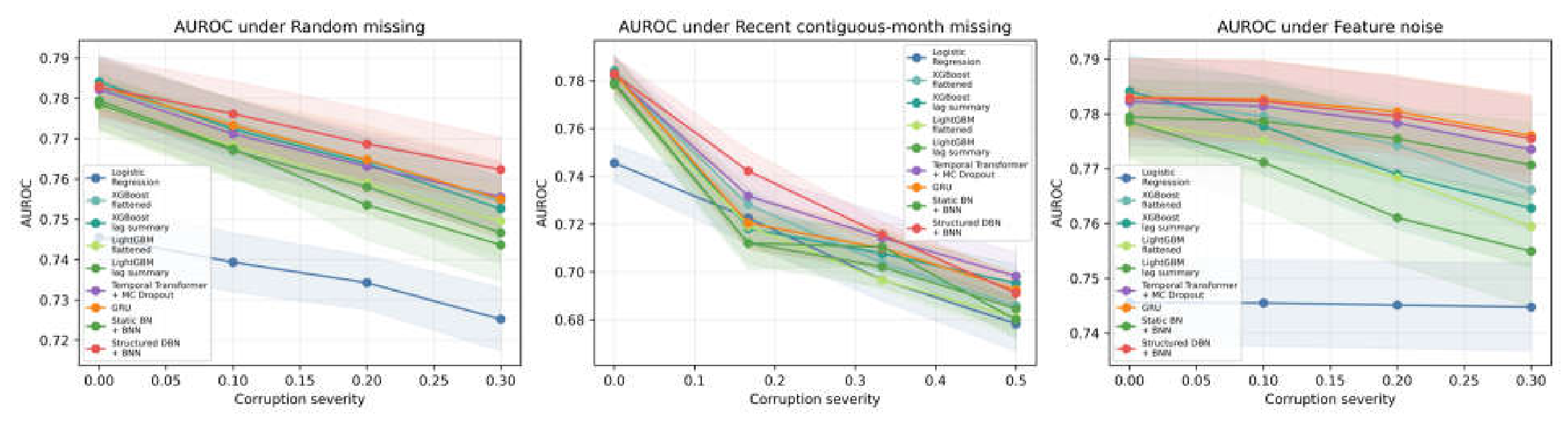
Figure 2 complements these fixed-severity comparisons by tracing AUROC across increasing random missingness, recent-block removal, and additive feature noise. The proposed model’s mean degradation from clean data is −0.0205 under 30% MCAR and −0.0406 after latest-month removal, compared with −0.0266 and −0.0504 for the Transformer. Under feature noise of severity 0.30, the proposed model achieves an AUROC of 0.7755 ± 0.0080, remaining comparable to the GRU at 0.7760 ± 0.0073 and the Transformer at 0.7735 ± 0.0092. The advantage is not universal under extreme information loss: when the three most recent months are removed, the Transformer reaches 0.6983 compared with 0.6912 for the proposed model. These results support robustness across several corruption settings rather than uniform superiority under every perturbation.
Table 3.
AUROC Across Clean Data and Four Missingness Mechanisms.
| Model | Clean | 30% MCAR | Latest month | 30% MAR | 30% MNAR |
|---|---|---|---|---|---|
| XGBoost (lag summary) | 0.7841 ± 0.0066 | 0.7527 ± 0.0078 | 0.7182 ± 0.0082 | 0.7531 ± 0.0082 | 0.7255 ± 0.0083 |
| Transformer + MC Dropout | 0.7822 ± 0.0079 | 0.7556 ± 0.0086 | 0.7318 ± 0.0098 | 0.7540 ± 0.0088 | 0.7239 ± 0.0090 |
| GRU | 0.7830 ± 0.0068 | 0.7550 ± 0.0095 | 0.7204 ± 0.0112 | 0.7544 ± 0.0097 | 0.7243 ± 0.0105 |
| Static BN + BNN | 0.7795 ± 0.0068 | 0.7436 ± 0.0088 | 0.7120 ± 0.0111 | 0.7468 ± 0.0088 | 0.7084 ± 0.0122 |
| Structured DBN + BNN | 0.7828 ± 0.0073 | 0.7623 ± 0.0080 | 0.7423 ± 0.0088 | 0.7611 ± 0.0088 | 0.7331 ± 0.0104 |
Mean ± standard deviation over ten evaluations. MAR and MNAR use a 30% target temporal missingness rate; no test-time adaptation was used. Bold indicates the best mean within the displayed models.
3.5. Calibration, Selective Prediction, and Sensitivity
Table 4.
Probability Quality and Threshold Utility Under Missing Evidence.
| Condition | Model | Brier | ECE | F1 |
|---|---|---|---|---|
| 30% MCAR | Transformer + MC Dropout | 0.1436 | 0.0404 | 0.4756 |
| 30% MCAR | GRU | 0.1432 | 0.0314 | 0.4946 |
| 30% MCAR | Static BN + BNN | 0.1449 | 0.0249 | 0.4768 |
| 30% MCAR | Structured DBN + BNN | 0.1409 | 0.0274 | 0.5062 |
| Latest month | Transformer + MC Dropout | 0.1555 | 0.0754 | 0.4028 |
| Latest month | GRU | 0.1555 | 0.0670 | 0.4212 |
| Latest month | Static BN + BNN | 0.1604 | 0.0748 | 0.3395 |
| Latest month | Structured DBN + BNN | 0.1489 | 0.0511 | 0.4512 |
Under 30% MCAR, the proposed model achieves the lowest Brier score and highest F1, while Static BN + BNN has the lowest ECE. After latest-month removal, the proposed model performs best on all three metrics. At 10% selective coverage, it yields the lowest error (3.51% ± 0.99%), compared with 3.82% for the Transformer, 4.09% for GRU, and 4.34% for Static BN + BNN; at 20% coverage, its 5.15% error is close to the Transformer’s 5.10%. The effective latent-state count is 10.77 ± 0.42. In the exploratory seed-42 analysis, AUROC ranges from 0.7714 to 0.7757 across K ∈ {4, 8, 12, 16, 24}, with Brier and ECE ranges of 0.1359–0.1390 and 0.0109–0.0340. AUROC varies by at most 0.0008 across tested prior, KL, and reconstruction settings, whereas ECE ranges from 0.0177 to 0.0300, indicating stable ranking but greater calibration sensitivity. Error at fixed coverage does not establish the lending-profit improvements targeted by profit-based rejection methods [24].
3.6. Computational Cost and Scalability
All runtimes were measured in the same CPU-only Windows environment. Structured DBN + BNN required 271.2 ± 159.3s for training and contained 177,650 parameters, versus 106.3 ± 69.3s and 11,425 parameters for the Transformer, 63.0 ± 32.7s and 18,177 for GRU, and 38.8 ± 24.4s and 8,206 for Static BN + BNN. The proposed model was therefore 2.55 times slower than the Transformer and 4.30 times slower than GRU. With 100 Monte Carlo samples and batch size 256, median CPU inference latency was 146.9ms, or approximately 1,743 customers/s.
In the single-seed scalability analysis, using 25%, 50%, and 100% of the training data required 35.9, 52.2, and 310.6s and achieved AUROCs of 0.7623, 0.7698, and 0.7757. These results illustrate the accuracy–cost trade-off but do not establish linear scaling because early stopping and CPU workload affect runtime.
4. Conclusions
This study introduced a Structured DBN + BNN for uncertainty-aware credit-risk prediction from longitudinal borrower records. Across ten paired seeded evaluations, the model achieved competitive complete-data discrimination (AUROC 0.7828) and showed its clearest advantage when temporal evidence was incomplete. Under 30% MCAR missingness, AUROC remained 0.7623, while uncertainty-based selective prediction reduced error to 3.51% at 10% coverage. Ablation results indicate that explicit temporal transitions and training-time denoising, rather than reconstruction alone, provide the main robustness gains.
The evaluation is limited to one public dataset with six monthly observations, and all missingness mechanisms are synthetic. Because institution identifiers and absolute application or cohort dates are unavailable, genuine cross-institutional or temporally separated validation could not be performed. Repeated holdouts overlap, extreme recent-block missingness remains challenging, latent states are diagnostic rather than causal, and the variational posterior only approximates parameter uncertainty. The model also incurs higher computational cost than simpler baselines. External validation under naturally occurring missingness, calibration drift, and institutional or temporal distribution shifts remains necessary before deployment.
References
- Hand, D.J.; Henley, W.E. Statistical Classification Methods in Consumer Credit Scoring: A Review. J. R. Stat. Soc. Ser. A (Statistics Soc. 1997, 160, 523–541. [CrossRef]
- Lessmann, S.; Baesens, B.; Seow, H.-V.; Thomas, L.C. Benchmarking state-of-the-art classification algorithms for credit scoring: An update of research. Eur. J. Oper. Res. 2015, 247, 124–136. [CrossRef]
- Zhang, X.; Yu, L. Consumer credit risk assessment: A review from the state-of-the-art classification algorithms, data traits, and learning methods. Expert Syst. Appl. 2023, 237. [CrossRef]
- Zhang, W.; Lim, M.K.; Yang, M.; Li, X.; Ni, D. Using deep learning to interpolate the missing data in time-series for credit risks along supply chain. Ind. Manag. Data Syst. 2023, 123, 1401–1417. [CrossRef]
- Ghahramani, Z. AN INTRODUCTION TO HIDDEN MARKOV MODELS AND BAYESIAN NETWORKS. Int. J. Pattern Recognit. Artif. Intell. 2001, 15, 9–42. [CrossRef]
- C. Blundell, J. Cornebise, K. Kavukcuoglu, and D. Wierstra, “Weight uncertainty in neural networks,” in Proceedings of the 32nd International Conference on Machine Learning, vol. 37, pp. 1613–1622, 2015. Available: https://proceedings.mlr.press/v37/blundell15.html.
- Nagl, M.; Nagl, M.; Rösch, D. Quantifying uncertainty of machine learning methods for loss given default. Front. Appl. Math. Stat. 2022, 8. [CrossRef]
- C. Guo, G. Pleiss, Y. Sun, and K. Q. Weinberger, “On calibration of modern neural networks,” in Proceedings of the 34th International Conference on Machine Learning, vol. 70, pp. 1321–1330, 2017. Available: https://proceedings.mlr.press/v70/guo17a.html.
- X. Han and Y. Xiao, “Decomposing firm-level crisis responses from incomplete market signals: Evidence from China’s IT sector during COVID-19,” arXiv:2606.10297, 2026. [CrossRef]
- Krishnan, R.; Shalit, U.; Sontag, D. Structured Inference Networks for Nonlinear State Space Models. Proc. AAAI Conf. Artif. Intell. 2017, 31. [CrossRef]
- S. M. Lundberg and S.-I. Lee, “A unified approach to interpreting model predictions,” in Advances in Neural Information Processing Systems, vol. 30, 2017. Available: https://proceedings.neurips.cc/paper/2017/hash/8a20a8621978632d76c43dfd28b67767-Abstract.html.
- C. Wu and Y. Lin, “Evidence-unit fairness and the limits of query-adaptive sparse-dense fusion in financial document retrieval,” arXiv:2608.00183, 2026. [CrossRef]
- Pozzolo, A.D.; Boracchi, G.; Caelen, O.; Alippi, C.; Bontempi, G. Credit Card Fraud Detection: A Realistic Modeling and a Novel Learning Strategy. IEEE Trans. Neural Netw. Learn. Syst. 2017, 29, 3784–3797. [CrossRef]
- Q. Yan, “Temporal heterogeneous graph transformer for credit card fraud detection,” arXiv:2609.07100, 2026. [CrossRef]
- Bahnsen, A.C.; Aouada, D.; Ottersten, B. Example-dependent cost-sensitive decision trees. Expert Syst. Appl. 2015, 42, 6609–6619. [CrossRef]
- G. Papamakarios and I. Murray, “Fast ε-free inference of simulation models with Bayesian conditional density estimation,” in Advances in Neural Information Processing Systems, vol. 29, pp. 1028–1036, 2016. Available: https://proceedings.neurips.cc/paper/2016/hash/6aca97005c68f1206823815f66102863-Abstract.html.
- R. Zhang, O. A. Chkrebtii, and D. Xiu, “Likelihood-free posterior density learning for uncertainty quantification in inference problems,” arXiv:2508.00167, 2025. [CrossRef]
- Y. Zhu and R. Zhang, “AIM: Amortized inference for multistate transition models,” arXiv:2607.23294, 2026. [CrossRef]
- Z. Zheng, B. Li, J. Yao, and J. Long, “Reliable financial named entity recognition under domain shift: Confidence estimation and selective prediction,” arXiv:2608.19558, 2026. [CrossRef]
- Smirnov, V.S.; Stupnikov, S.A. A Deep Learning Approach to Credit Scoring Using Credit History Data. Lobachevskii J. Math. 2023, 44, 198–204. [CrossRef]
- Korangi, K.; Mues, C.; Bravo, C. A transformer-based model for default prediction in mid-cap corporate markets. Eur. J. Oper. Res. 2022, 308, 306–320. [CrossRef]
- Zhao, F.; Lu, Y.; Li, X.; Wang, L.; Song, Y.; Fan, D.; Zhang, C.; Chen, X. Multiple imputation method of missing credit risk assessment data based on generative adversarial networks. Appl. Soft Comput. 2022, 126. [CrossRef]
- Xu, Y.; Kou, G.; Peng, Y.; Ding, K.; Ergu, D.; Alotaibi, F.S. Profit- and risk-driven credit scoring under parameter uncertainty: A multiobjective approach. Omega 2023, 125. [CrossRef]
- Pang, M.; Wang, F.; Li, Z. Credit risk prediction based on an interpretable three-way decision method: Evidence from Chinese SMEs. Appl. Soft Comput. 2024, 157. [CrossRef]
- Xu, Y.; Kou, G.; Ergu, D. Profit-based uncertainty estimation with application to credit scoring. Eur. J. Oper. Res. 2025, 325, 303–316. [CrossRef]
- Yeh, I.-C.; Lien, C.-H. The comparisons of data mining techniques for the predictive accuracy of probability of default of credit card clients. Expert Syst. Appl. 2009, 36, 2473–2480. [CrossRef]
Figure 1.
Architecture of the proposed Structured DBN + BNN. The static-conditioned DBN and complementary GRU/MLP encoders feed a feature-fusion module and variational BNN; the dashed reconstruction branch is used only during training.
Figure 1.
Architecture of the proposed Structured DBN + BNN. The static-conditioned DBN and complementary GRU/MLP encoders feed a feature-fusion module and variational BNN; the dashed reconstruction branch is used only during training.
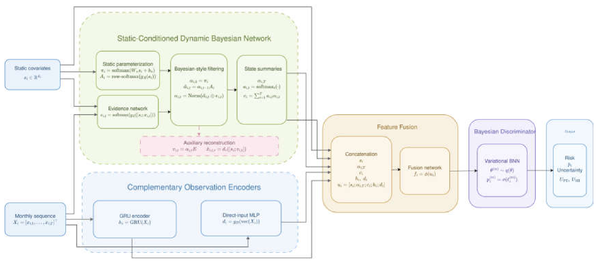
Figure 2.
Mean AUROC versus corruption severity under random missingness, recent contiguous-month removal, and Gaussian feature noise. Solid lines and shading show means ±1 SD over ten paired seeded evaluations. Recent-block severities 1/6–3/6 remove the last one to three months; noise severity is its standard deviation.
Disclaimer/Publisher’s Note: The statements, opinions and data contained in all publications are solely those of the individual author(s) and contributor(s) and not of MDPI and/or the editor(s). MDPI and/or the editor(s) disclaim responsibility for any injury to people or property resulting from any ideas, methods, instructions or products referred to in the content. |
© 2026 by the authors. Licensee MDPI, Basel, Switzerland. This article is an open access article distributed under the terms and conditions of the Creative Commons Attribution (CC BY) license (http://creativecommons.org/licenses/by/4.0/).
Copyright: This open access article is published under a Creative Commons CC BY 4.0 license, which permit the free download, distribution, and reuse, provided that the author and preprint are cited in any reuse.