

Submitted:
20 September 2026
Posted:
21 September 2026
You are already at the latest version
Abstract
We study a critical homogeneous continuous-time Markov branching-immigration system whose offspring and immigration generating functions are regularly varying at the point~1 of orders \(1+\nu\) and \(\delta\) with \(\nu,\delta\in(0,1]\), the slowly varying factors being controlled through their index functions. Two numbers govern the classification: the difference \(\gamma=\delta-\nu\) of the two orders and the limit \(\Lambda_{\infty}\) of the ratio of the immigration factor to the offspring one. We classify the state space completely: positive recurrent for \(\gamma>0\), transient for \(\gamma< 0\), and on the boundary \(\gamma=0\) null recurrent or transient according as \(\Lambda_{\infty}\le{\nu}\) or \(\Lambda_{\infty}>\nu\), which at \(\nu=\delta=1\) reduces to the classical threshold. In each regime we identify the limiting generating function of the normalised transition functions together with the exact rate of convergence to it, uniformly in the argument on compact subsets of [0,1), the transient rate under two further inequalities on the parameters; and we carry every rate to the individual transition probabilities, with no monotonicity hypothesis, by a complex-analytic argument resting on a factorisation that criticality forces. The constants are made accessible by an exact integral identity for the survival probability of the system without immigration, which also yields a three-term expansion of that probability in closed form. A numerical section on explicit models confirms the constants and the rates.
Keywords:
Markov branching system
; criticality
; immigration
; regular variation
; index function
; state classification
; null recurrence
; invariant measure
; strong ratio limit property
; local limit theorem
; rate of convergence
MSC: 60J80; 60J27; 60F05; 26A12
1. Introduction
Branching systems are among the oldest and most persistent models of population growth, and the continuous-time Markov branching system is the member of the family in which the interplay between reproduction and time is the most transparent: an individual alive at time t waits an exponential time and is then replaced by a random number of offspring, independently of everything else. Throughout the paper t is time and runs over the axis , while s is the argument of a generating function and runs over ; both are fixed formally in Section 2, and s is allowed to be complex only in Section 9 and in the numerical check of its bounds in Section 10. Adding an immigration stream, so that new individuals enter the population at the epochs of an independent Poisson-type mechanism, turns the model into a genuinely different object. The population can no longer become extinct in the absolute sense, and the question of long-time behaviour becomes a question about the recurrence structure of an irreducible Markov chain on the nonnegative integers. Classical accounts are given in [3,14,36], and the immigration model itself goes back to Sevastyanov [35], Yang [40] and Pakes [30]; in discrete time see Foster and Williamson [10] and Zubkov [42], and, for the process stopped at the origin, Ivanoff and Seneta [21].
The critical case, in which the mean offspring number per individual is exactly one, is at the same time the most delicate and the most informative. Under a second moment condition on the offspring law and a first moment condition on the immigration law, Sevastyanov [35] and Pakes [30] showed that the transition functions decay polynomially and that a limiting generating function exists after multiplication by , where is the ratio of the immigration mean to half the offspring variance. The power series expansion of that limit generates an invariant measure; for the system without immigration the corresponding structure is the theorem of Kesten, Ney and Spitzer [23]. Li, Chen and Pakes [25] refined the picture considerably, and Imomov [15] added rates of convergence under finiteness of the third derivative of the offspring generating function and of the second derivative of the immigration one.
Once the second moment of the offspring law is infinite the classical normalisation collapses, because the constant that drives it is no longer defined. The natural replacement is a regular variation hypothesis: the offspring generating function and the immigration generating function are taken regularly varying at the point 1, of orders and with and with slowly varying factors and . These are the hypotheses , of Section 2, where both functions are written out in full; the classical case is . Besides the two orders, one number built from the slowly varying factors will matter throughout, the limit , introduced formally at (13). In discrete time, limit theorems for the critical process with immigration and infinite offspring variance go back to Pakes [31], and regularly varying immigration has been taken up more recently in [4,5]. This exact setting was worked out in [18,25], where it was shown that the sign of the single parameter separates a recurrent from a transient regime, and four of the present authors [17] developed the transient side of that dichotomy in detail; rates of convergence in the two regimes were taken up in [16]. That line of work leaves open the boundary between the two regimes, the normalisation of the transient one and the control of the slowly varying factors, and the present paper answers all three.
Nothing is said there about the boundary , which is precisely the stratum containing the classical case ; and the classical case is known to split further, into a recurrent and a transient part, according to the size of . One expects a dichotomy on the whole of the boundary, and we prove that there is one: for the state space is null recurrent when and transient when , with as above. At this reduces exactly to the classical threshold. Together with the two open regimes this gives a complete classification of the state space, stated as Theorem 6 below.
In the transient regime it is the normalisation that has to be corrected. When the transition functions decay at a stretched exponential rate, and the correct normalising factor is with
where is the reciprocal of the survival probability of the branching system without immigration. With the simpler factor used there, the limit exists only under the additional hypothesis , which cuts a null set out of the parameter space. Carrying the constant through the normalisation costs nothing and removes the hypothesis altogether; this is Theorem 7.
The slowly varying factors themselves call for a control of a different kind. The standard device is to postulate a remainder in the shift relation and then to suppress the dependence of on the shift . The suppression has a cost. All of the estimates in this circle of problems are driven not by but by the index function of the representation theorem, and the two are proportional with a factor that depends on and is not identically equal to one. We therefore state the hypotheses directly in terms of the index function, and record the relation to the shift remainder as a lemma. The gain is not only cleanliness. The identity that the index function satisfies is exact, and the exact identity, given as Lemma 3 below, produces a three-term asymptotic expansion of the survival probability,
in which is the limit of the slowly varying factor of the offspring generating function, is the limit of times its index function, and is a constant built from the same data; all three are written out in terms of alone in Theorem 2. When is constant the exact identity behind this expansion degenerates to , where is the auxiliary function introduced at (12) below, which is both elementary and classical; it is for a genuinely varying , including a non-constant one with , that the expansion has content. A two-term form of it, with a logarithmic correction of the same shape but retaining an implicitly defined norming function, is [17, Thm. 1]; the coefficient carried there is the present one at , which is a hypersurface of the parameter space and not an identity, and Remark 2 says where the difference comes from. What is added here is the third term, the constant , and the removal of the norming function, which is what makes the expansion usable as it stands.
Beside this line of work should be placed the recent paper of Mitov and Yanev [28], which carries the same two regular variation hypotheses into a wider model: immigration there occurs at the jump epochs of a Poisson process of intensity with tending to a positive constant, so that the present system is the case of an intensity constant throughout, their offspring order being our and their immigration order our . Their companion papers [27,29] treat the same model with an increasing intensity and with one tending to zero, and the present system is a case of neither. The results of [28] touch ours at four places, and only two of them concern a statement proved below, in each case on a stratum that was already known. Their criterion separates from by the convergence of an integral, which is the positive recurrent stratum of Theorem 6(i); the splitting of the boundary into a null recurrent and a transient part is not addressed there, and it is that splitting which Theorem 6(ii) supplies. On that same boundary they obtain a proper limit law for the population size divided by , of Laplace transform for , and their divergent case covers the transient stratum as well, yielding there a stable limit law for the population size under its own normalisation. These two limit laws are statements in which the argument of the generating function approaches 1 as t grows, and they are complementary to Theorems 10 and 7 below, which keep the argument fixed and describe the invariant measure. Their convergent case yields for the limiting generating function of Theorem 11 below, without a rate; that limit is not new here either, and the head of Section 8 says where it does come from. The one regime of [28] that does not arise here at all is that in which the ratio of the two slowly varying factors degenerates: the standing hypotheses of Section 2 force its limit to be finite and positive.
The rest of the paper is arranged as follows. Section 2 describes the model, fixes the Karamata classes in Section 2.2 and states the standing hypotheses. Section 3 is devoted to the exact identity and to the Basic Lemma of the critical branching system that follows from it, together with the survival probability, the local probability of finding that system in state 1, and the generating function of the invariant measure of the branching system without immigration. Section 4 stays with that system and gives rates for the conditioned transition functions and for the local ratios. Section 5 returns to the system with immigration and contains the classification theorem, and Section 6, Section 7 and Section 8 treat, in turn, the transient regime , the boundary and the positive recurrent regime ; each of them identifies the limiting generating function and the exact rate of approach to it. Section 9 carries every rate of the paper from the generating functions to the individual transition probabilities, by a complex-analytic argument resting on a factorisation that criticality forces and needing no monotonicity hypothesis. Section 10 carries out a numerical verification on explicit models in which every constant of the paper can be computed independently. Section 11 collects concluding remarks and the questions that remain open.
It remains to say how the present paper stands to the treatment of [17], of which it is the direct continuation. Section 2, Section 3 and Section 4 revisit material treated there; we have retained only what the new results need, and in each case the statement given here supersedes its earlier counterpart. The hypotheses are now placed on the index functions of the two slowly varying factors rather than on their shift remainders; the two formulations are related by Lemma 2, and the constants of the earlier one are to be read through the factor appearing there. The implicitly defined normalising function of that treatment is superfluous under the present hypotheses and has been replaced throughout by the explicit constant ; see Remark 2. The normalisation of the transient regime carries the constant , so that the hypothesis of the earlier version is not needed.
The generating function of the invariant measure of the system without immigration is given here by Corollary 1. Its last term is absent from the expression stated as [17, Thm. 7], which therefore holds as an identity precisely when is constant, and in particular in the classical finite variance case, where the distinction does not arise; for a genuinely varying the two differ by a factor of the order of unity which tends to 1 only as , as Section 10 shows. The statements of Section 4 that rest on are restated accordingly. The range of the indices is also wider, both being allowed to take the value 1: the earlier treatment assumes , so that the classical finite variance case lies outside its range, whereas here it is a point of the boundary stratum and is covered by Theorem 10.
Nor is any normalisation imposed on the constants. In that treatment the shift remainders of the two slowly varying factors are written and , the two constants and are formed from them, and the constant that governs the transient regime is their ratio , on which the hypothesis of that regime is imposed. The constant that governs the same regime here is of (13), the ratio of the two limits and . The two agree, but only because the remainders are narrowed there by as and its analogue for , which force and . That these are hypotheses and not identities is what (10) below shows: it gives
the second by the analogue of (10) for under . Each narrowing is therefore a relation between two of our four constants, depending on the shift besides, and together they cut a set of codimension two out of the parameter space. Under the Basic Axioms nothing of the kind is assumed: , , and are independent and enter the results separately, and the ratio is then not .
Section 5, Section 7, Section 8, Section 9 and Section 10 have no counterpart in [17]. Some of them, and also Section 4, have one elsewhere, and the boundary between what is taken over and what is added should be said plainly. The classification of Section 5 is the evaluation, under the standing hypotheses, of a criterion that is classical and is recalled at (52) below; its content is the boundary stratum, the two other strata being the dichotomy already read off from that criterion in [18,25]. The limiting generating function of the positive recurrent regime of Section 8 is that of [18, Thm. 1.2], and the rate of approach to it, with its constant, is [16, Thm. 2.1]; what is added there is a rate expressed in constants rather than in slowly varying factors, the monotonicity and the uniformity of the approach, and the passage to the transition probabilities. The two limits of Section 4, finally, are, up to notation, [17, Thms. 8, 9], with there in the reduced form that Corollary 1 corrects; what is added there is the second-order correction of Theorem 4 below, its uniformity in s, and the transfer to the individual probabilities. The head of each of the three sections points back to here.
2. The Model and the Standing Hypotheses
2.1. The Branching-Immigration System
Let be the set of natural numbers, let and let be the time axis. We consider a population of monotype individuals. Each individual alive at time , independently of its history and of all other individuals, is transformed during according to the rule that it produces offspring with probability , and with probability either survives without reproducing or produces exactly one offspring, all as . The branching rates satisfy for together with the consistency condition
Independently of the branching mechanism, new individuals enter the population during with probability , and no immigration occurs with probability , again as . The immigration intensities satisfy for and . Immigrants reproduce according to the same branching rates. The two mechanisms are encoded by the infinitesimal generating functions
for . Both vanish at , and , . The resulting stochastic model is called the continuous-time Markov branching-immigration system, abbreviated MBIS. Its relation to the discrete-time model is the embedding problem of Karlin and McGregor [22].
Write for the population size at time . The process is a homogeneous continuous-time Markov chain on a state space with transition functions
for and ; here t is the length of the transition interval and not an infinitesimal quantity. We take to be the set of states reachable from 0. Because , every line of descent can die out, so that 0 is reachable from each state of ; hence is a single communicating class and the chain is irreducible on it. One has as soon as , and nothing below depends on which subset is. The chain is also honest, that is non-explosive: the total jump rate of an individual is , the total immigration rate is , and in the critical case the branching part cannot explode; see [3, Ch. III] and [2, Ch. 2]. The generating function is a power series with nonnegative coefficients of sum at most 1, so that it converges absolutely on the closed unit disc and is analytic on the open one, and the same holds for below. The remaining generating functions of the paper have nonnegative coefficients as well, and each is shown analytic on where it is introduced. We nevertheless write the argument as a real throughout, the sole exception being Section 9, where the extension to complex s is precisely what carries the results to the individual transition probabilities. The generating function admits the representation
where solves the backward
and the forward
Switching the immigration off amounts to , that is, to for every . What remains is the Markov branching system without immigration, abbreviated MBS, whose population size we denote by . It is a reducible chain on with a communicating class of transient states and absorbing, and
and . Thus is common to both systems, and (1) exhibits the MBIS as the immigration stream superposed on it. The extinction probability of the MBS is the smallest root of in , and converges to it as , uniformly in for each ; see [30].
Differentiating (1) at gives
where and, here and throughout, the argument marks the limit as the variable increases to 1. Formula (4) shows that the growth of the mean is governed by the sign of a alone: the system is subcritical, critical or supercritical according as , or , and in the first two cases the extinction probability equals 1. Throughout the paper the system is critical, so that
In particular on , because is convex with ; and on , because is nondecreasing with and . Finally, (1) shows that as for every , the extinction probability being 1, so that it suffices throughout to study
whose value at is the return probability .
2.2. Karamata Classes and the Index Function
A positive measurable function defined on a neighbourhood of infinity is slowly varying at infinity if as for every ; the class of such functions is denoted . A function is regularly varying at infinity with index , written , if for some . The representation theorem states that every can be written as
with and as ; if is constant then is called normalised, and in that case is differentiable with
We call the index function of . All slowly varying functions occurring below are normalised, so that the index function is defined; see [6, §1.3].
Most of the literature on branching systems controls the fine structure of not through the index function but through a remainder in the shift relation, one writing and postulating a decay rate for , after which the subscript is suppressed and is treated as a single function; the subclass of so obtained is recalled at (7) below, where our own hypotheses are placed inside it. Both devices have been used, and the passage between them, with the classification of remainders it induces, is the subject of [20]. What is not harmless is the suppression of : it is a notation and not an identification, since what the proofs actually use is the index function, and the two are proportional with a factor that depends on the shift and is not identically unity, as Lemma 2 below makes precise. We therefore place the hypotheses on the index function itself throughout.
2.3. Standing Hypotheses
The generating functions are assumed regularly varying at the point 1:
and
for , where and are normalised. Hypothesis says that the offspring law lies in the domain of attraction of a -stable law, the hypothesis under which the theory of the critical system without immigration has been developed since Slack [37] and Seneta [34]; see also Vatutin [39] and Pakes [33]. It forces when , while with tending to a positive limit as is the finite variance case, being twice that limit. Hypothesis says that the immigration law has finite moments of every order below and, once is bounded away from zero at infinity, as it is under below, infinite moment of order when , while with as is the finite immigration mean case. Two parameters control everything that follows:
The fine structure of the two slowly varying factors is controlled by their index functions. We assume
and
Where an exact remainder is needed we strengthen these to their quantitative forms
and
for some and , and we write
for the joint rate they produce. Hypotheses , , and together are referred to as the Basic Axioms.
The two constants and are allowed to vanish, and the case in which both do is not a degenerate one but the classical one: for and constant the index functions vanish identically, so that , and at is the finite variance case. Nothing below is empty there: the expansion (29) below simply loses its logarithmic term, and the rate (75) below keeps the constant it has. Positivity is required at exactly two points of the paper, and is hypothesised there rather than here: in Lemma 2, where the index function is divided by the shift remainder, and in Theorem 7, where it is what makes the leading term of the transient rate the one displayed; what happens at is written out in Remark 7.
Hypotheses and are quantitative statements of membership in the Karamata subclass of slowly varying functions with remainder. Given a positive nonincreasing function with as , a function is said to be slowly varying with remainder , written , if
for every ; this is condition SR1 of [6, Ch. III,§3.12.1], the class and its calculus going back to Bojanic and Seneta [7], to Aljančić and Arandjelović [1] and to Goldie and Smith [12]; see also Geluk and de Haan [11]. The asymptotic theory of the critical branching system with infinite offspring variance has been developed precisely in this subclass, with the calibration for the offspring factor and for the immigration one; see [18, Thms. 1.2, 1.3] and the hypotheses preceding them. In that calibration, membership in is, by [6, Cor. 3.12.3], equivalent to as , so that the finite positive limit is forced by the subclass itself and is not an extra assumption; Lemma 1 below obtains the same conclusion from the index function.
Our axioms lie inside that subclass, and Lemma 2 makes the inclusion explicit: gives with the exact constant in place of the of (7), and the same holds for with and in place of and under . Two things are gained by placing the hypotheses on the index function rather than on the remainder of (7). The remainder of (7) depends on the shift while the index function does not, so that every constant obtained below is shift-free; and the second-order rates , of and have no counterpart in (7), whose carries no constant at all; it is these two rates, through of (6), that turn every of the paper into an explicit power of t.
It should be said at once what the Basic Axioms do and do not allow. By Lemma 1 below, hypothesis forces to have a finite positive limit, so that together with is a condition of regular variation of the second order in the sense of de Haan and Stadtmüller [13],
rather than a condition of plain regular variation: a factor such as is excluded. What is retained is the essential feature of the problem, namely for , and what is gained is that every constant below is finite and explicit. The same remark applies to and . Hypotheses of this kind are exactly those under which the shift remainder of the earlier formulations decays at the rate postulated there; see Lemma 2 and Remark 1.
Two consequences of the Basic Axioms are used constantly and are recorded at once.
Lemma 1.
Let hold. Then the limit exists in and
If moreover holds, then the in (8) is . Finally
as , uniformly in . The same statements hold for with ν, , replaced by δ, , , the limit being denoted .
Proof.
By we have as , so that the integral
converges absolutely. Since
the limit exists and is finite, and it is positive because the exponent is bounded. In the shift-remainder formulation the same conclusion is known; see [19]. Writing
and using as together with
gives (8); the quadratic term of contributes , which is . The additive form is the one needed: the constant is allowed to vanish by , and a relative remainder would then assert that is constant. Under the last display carries the remainder , and together with the quadratic term this is the asserted bound. Finally , and the first half of (9) follows because is bounded and as ; the second half is the first integrated over , the integrand being of the constant order throughout . □
Lemma 2.
Proof.
Remark 1.
Relation (10) shows that the shift remainder does carry the decay rate postulated in the earlier formulations, so the Basic Axioms in the present form are at least as strong as those of the earlier formulations discussed in Section 1. Relation (11) shows in what sense they are more precise. The factor depends on the shift and exceeds ν for every , taking the value 1 only on the curve of the parameter plane, and never at all when . The index function and the shift remainder can therefore not be identified with one another: a constant computed by replacing one with the other differs from the true one by that factor. Working with from the outset removes the difficulty, and with it the arbitrariness of the choice of μ.
We shall also use throughout the two auxiliary functions
for and , together with the constant
whose existence is guaranteed by Lemma 1. The constant of (13) is the single number through which the immigration mechanism enters every limit theorem below. Hypothesis gives
Finally we record, for later use, the elementary consequence of Lemma 1 that
which is obtained by writing
and inserting (8) and its analogue for . The bracket in (15) may vanish identically, as it does when and , and in particular in the classical case ; this is why the remainder there is additive and not relative. If moreover and hold, then the same computation carried one step further sharpens the o-term of (15) to an explicit power,
with of (6): by Lemma 1 the two numerators carry the errors and , and the expansion of about contributes .
3. The Basic Lemma of the Critical Branching System
Throughout this section we work with the critical MBS generated by the infinitesimal generating functions alone, and with
together with the abbreviations
The quantity is the survival probability of the system started by a single ancestor. A statement describing the asymptotic behaviour of is traditionally called the Basic Lemma of the theory of critical branching systems; under hypotheses of the present kind it goes back to Zolotarev [41] in continuous time and to Slack [37] and Seneta [34] in discrete time. We shall obtain it from an identity that is exact, and it is the exactness that makes the constants below accessible. We need the generating function of the invariant measure of the MBS,
the second equality following from and the substitution . Its coefficients are written throughout, so that for ; that is analytic on the whole unit disc, and hence that the expansion converges there, is part of Lemma 9 below, whose proof uses nothing from the intervening sections. Together with it we use the integral
which is finite for every and nondecreasing when .
Lemma 3.
Let hold. Then for every and every
Proof.
Identity (19) is exact; it involves no asymptotics and no hypothesis beyond . Everything in this section is read off from it once the growth of is known. Put
Lemma 4.
Let hold. Then
If in addition holds, then the constant
is finite and
Proof.
Recall the notation (20) and write the integrand of (18) as
which is legitimate because . By and Lemma 1 the second factor tends to , and (21) follows on integrating. Under the deviation of that factor from its limit is
by Lemma 1. Dividing by x produces an absolutely integrable function on , so is finite, and the tail of the integral is , which is (23). □
Lemma 4, and likewise every tail estimate of Section 6, Section 7 and Section 8, is the index-function counterpart of the general asymptotics of integrals of Karamata functions with a controlled remainder, for which see [7,12] and [6, §3.12]; we prove the versions we need inline, because what is wanted here is not the order of the tail but the exact constant in front of it, and that constant is or rather than the shift remainder. Combining Lemmas 3 and 4 gives the Basic Lemma in the form in which it will be used.
Theorem 1.
Let and hold. Then, uniformly in for every ,
If in addition holds, then the remainder is exact:
uniformly in .
Proof.
Insert (21) and (23) into (19). For the uniformity note that for and , so that
since on , identity (19) read together with (26) forces uniformly on , and in particular
uniformly on . That is of exact order is the content of (28) in Theorem 2 below, and with (27) it turns the remainder of (23) into the uniform of (25). The proof of Theorem 2 uses (19) at and (21) only, so that the order of proof is (19), (21), (28), (24) and there is no circularity. □
The choice in Theorem 1, for which and , yields the survival probability. The expansion below has three terms and no unspecified constants.
Theorem 2.
Let and hold. Then
If in addition holds, then
where the constant, built from of (22), is
and equivalently
Proof.
Remark 2.
Under the Basic Axioms the auxiliary function is superfluous: by Lemma 1 the slowly varying factor has a finite positive limit, so that as and the normalisation is the explicit power . We therefore do not use anywhere below.
The comparison extends to the second term, and there the two accounts differ. Written in the notation of (20), the logarithmic correction of [17] is the one carried by (29) and (31) when , whereas under the Basic Axioms ϑ is a free constant of the offspring generating function, equal to the limit of ; Model T of Section 10 has . The origin of the difference is the one recorded in Remark 1. The hypothesis there is imposed on the shift remainder and reads as ; by (11) that hypothesis gives , a quantity which still depends on the shift, and the value is what the further identification of with produces. The coefficient is open to inspection in a closed-form model, as Section 10 shows.
The comparison of with is needed in each of the sections that follow, and is recorded here once.
Lemma 5.
Let hold. Then for every and every
an identity in which the logarithmic terms of Theorem 1 cancel. If in addition holds, then the bracket in (33) is and, uniformly in for every ,
and
In particular, uniformly in ,
Proof.
Subtracting (19) at from (19) at s gives (33). Let now hold and fix . The integrand of is times , and the latter is bounded by and Lemma 1; hence, with a constant and uniformly on ,
Since uniformly on , as shown in the proof of Theorem 1, the bracket in (33) is bounded, so that is bounded too; as has a finite positive limit, uniformly on . Write and multiply (33) by ; since this reads
The mean value theorem applied to gives , because is nonnegative. By (37) the bracket term is therefore , and by (9) so is the last term, since
both uniformly on . Both are , so that , and the bracket is of the order , that is by (28). Solving for D now gives (34), the replacement of by costing by Lemma 1. Finally, by (34) and Theorem 2,
which is (35). Finally (36) is the mean value bound above read with , obtained above, and uniformly on by (26). □
We turn to the derivative of , which carries the local probabilities. Here too an exact identity is available.
Lemma 6.
Let hold. Then for every and
Proof.
Theorem 3.
Let and hold, and put . Then
and consequently
Proof.
Finally we record the generating function itself. Setting in Lemma 3 gives an identity that is worth isolating, because the form of enters the conditional limit theorems of Section 4.
Corollary 1.
Let hold. Then for every
Remark 3.
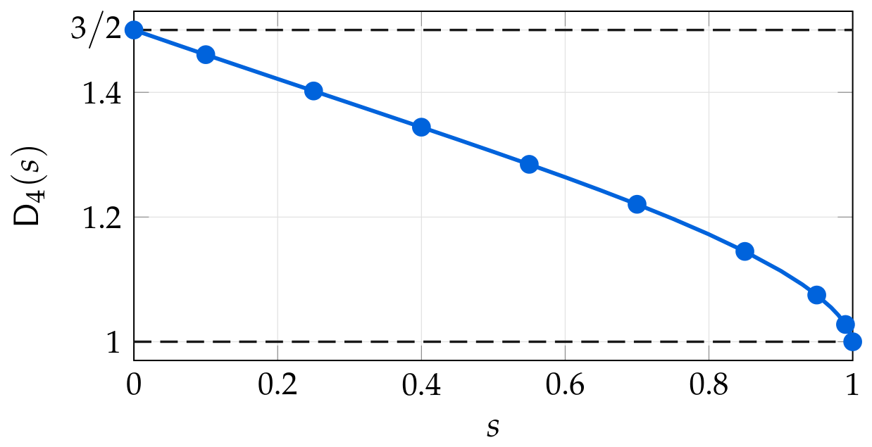
The term in (41) cannot be dispensed with. It vanishes identically if and only if is constant, which by and (14) means ; in the finite variance case one recovers the familiar . For a genuinely varying the reduced expression , obtained by suppressing that term, differs from by a factor of the order of unity rather than by a quantity of smaller order; the ratio of the two is given for Model T in Section 10. Since the two agree identically when is constant, the distinction is invisible in the finite variance theory and becomes visible only in the present generality.
It is also invisible in the limit . Under the omitted term is by (21), while grows like a power of ; the reduced expression is therefore the correct leading term of as , and the ratio of the two tends to unity, as Figure 3 shows for Model T. This is why the omission leaves untouched every statement in which enters asymptotically or is carried symbolically, and shows itself only when the formula is read as an identity at a fixed s. It is so read in [17, Thm. 7], where the term is absent from the displayed expression for ; (41) is the corrected form, and it is the one used throughout the present paper.
4. The Conditioned Branching System and Local Ratios
We stay with the MBS without immigration for one more section and record two consequences of Lemma 3 that are of interest in their own right and that sharpen the classical conditional limit theorems of [23,32,33,37,38]. The limits themselves are known in the present generality; what is taken over and what is added is set out in Section 1, and we do not repeat it. What is added here is the second-order correction of Theorem 4 below, quadratic in , together with the uniformity in s and the transfer to the individual probabilities. Set
the last equality being immediate from . It is convenient to abbreviate
the second equality being (25) at under .
Theorem 4.
Let and hold. Then, uniformly in for every ,
and the deviation in (43) is itself computable to one order more,
again uniformly in . If in addition holds, so that may be replaced by its expansion (42), then
uniformly in , the last term being the only part of the correction that carries a dependence on s.
Proof.
Write . By (12),
Identity (33) gives as . The second factor of (46) is not merely bounded: by (9) and the bound (36) of Lemma 5 it satisfies
uniformly on , the exact form of that factor being (48) below. Hence, as , one has , which is (43).
For (44) the two factors of (46) are needed one order further. In (33) the bracket is
by , so that by (35) the bracket equals . Consequently
For the second factor of (46), as , so that integration between the two arguments, using (34) and , gives
Write with (47), and expand the product of the two factors of (46) to order with (48). Taking the -th root by
the two terms in cancel, the two terms in combine with the coefficients and , and (44) follows, uniformly on . Nothing beyond has been used to this point, having been carried unexpanded. It remains, under , to multiply (44) by and to insert (42) together with (32), which gives (45). □
Remark 4.
The unnormalised form (44) is the sharper of the two, and it states the content of the theorem without constants: the deviation of from is asymptotically , quadratic in and negative. In the normalised form (45) the correction splits into a part free of s, namely the second-order term of the survival probability transported through , and the term , which is not. The latter is the first place at which the conditioned law is seen to approach its limit at a rate depending on the argument, and it is governed by alone. It does not disturb the ratio limit: dividing (45) at by the same relation at leaves with a relative error of order , so that the limit of the ratio is unaffected.
The corresponding statement for the ratios to is even simpler, because of the exact formula (38). Let
Theorem 5.
Let and hold. Then, uniformly in for every ,
so that as , with . The are nonnegative, being by Theorem 12 below the limits of the nonnegative ratios ; that theorem uses of the present one only (49), so the reference is not circular.
Read together with (40) of Theorem 3, the limit (49) is a local limit theorem for the branching system without immigration: writing one obtains
for each , the passage to the coefficients being legitimate by Theorem 12 below, which supplies it with a rate.
Remark 5.
One point about the conditioned system should be recorded. The conditioned probabilities are obtained by conditioning on the event separately for each , and this operation does not produce a time-homogeneous Markov chain: the conditioning event changes with t, so the family does not satisfy the Kolmogorov–Chapman equation. The Q-process, which conditions on non-extinction in the remote future, is a genuine Markov chain precisely because its conditioning event does not depend on t; see [24,32]. The statements (43) to (49), and those of Section 9, concern the conditioned distributions alone and use no Markov property of them, so nothing below depends on the point; we make it only to explain why no such property is invoked.
5. Classification of the State Space
We now return to the system with immigration. Everything rests on the following change of variable, which converts the time integral in (1) into an integral over the state variable and is used again in each of the three sections that follow.
Lemma 7.
Let and hold. Then for every and
Proof.
The three regimes of (51) are governed by the sign of , because the integrand is asymptotically : the integral diverges like a power of for , like a logarithm for , and converges for . This is the whole of the classification, and the threshold at the boundary is the coefficient of the logarithm.
The criterion that is being evaluated is classical, and it is worth writing down in order to see what the theorem below adds to it. The chain is irreducible and honest by Section 2, so that is recurrent if and only if and is positive recurrent if and only if has a positive limit as ; see [2]. Since is (1) at and the substitution , for which by (2), carries onto , the first of the two integrals is
In this form the criterion goes back to Pakes [30] and is developed in Chen and Renshaw [8] and in Li, Chen and Pakes [25]; the dichotomy between and is what reading it under and gives at once, and is recorded in [18,25]. The substance of the theorem below is therefore the boundary , where the sign carries no information and the two sides of (52) have to be separated by a second number; we state the three strata together because the classification is only complete when the boundary is included, and prove them from (51) at rather than from (52), the exponent of (51) being available to us in closed form.
Theorem 6.
Let the Basic Axioms hold. Then the state space of the MBIS is
- (i)
- positive recurrent if ;
- (ii)
- null recurrent if and , and transient if and ;
- (iii)
- transient if .
Proof.
We use the two criteria recalled above. By (51) at ,
and by Theorem 2, as .
Let . Since and , the integral in (53) converges as , so that tends to a strictly positive limit and (i) holds.
Let . Then (53) reads
and by (15) with the last integrand is , so that the last integral converges to a finite limit. Hence
for a constant , and diverges precisely when . Since as in either case, recurrence is null, and (ii) holds.
Let . Then and the integrand of (53) is at least for all large x, so that
eventually. As is of exact order with , the function decays at a stretched exponential rate and is integrable, so (iii) holds. □
Remark 6.
Part (iii) and the positive recurrence in part (i) recover the dichotomy of [18,25], itself the reading of (52) under the hypotheses and ; part (ii) is new and closes the boundary that the sign criterion leaves open. In [17] that stratum was set aside on the ground that forces and hence a different model, the Markov Q-process. The implication does not hold: says only that , and it leaves free, which is precisely why the stratum splits. It also reduces to the classical statement. Indeed, in the finite variance case with and as we have and , where λ is exactly the parameter of Sevastyanov [35] and Pakes [30], and the threshold becomes . Thus the classical criterion is the section of the boundary stratum at . Note also that the trichotomy is genuinely two-dimensional: on the boundary the sign of γ carries no information at all and the whole of the classification is done by .
6. The Transient Regime
Throughout this section , so that lies in , and we assume . By Theorem 6 the state space is transient and the transition functions decay at a stretched exponential rate. The correct normalisation is
and we introduce the three quantities
and
Both integrals in (56) converge. Indeed, by (15) the integrand is
because and ; it is therefore as , and suffices for convergence; and when the integrand is of exactly that order, so that is then also necessary. This is where the hypothesis enters, and, as long as , it is the only place.
The hypotheses and are needed already in the identity below, since enters the definitions (55)–(57) and the convergence of the two integrals (56) was read off from (15).
Lemma 8.
Let the Basic Axioms hold with and . Then for every and
where
Proof.
Split the integrand of (51), in which , into and
Identity (58) is exact. The theorem below merely evaluates the two terms in its exponent. Note that (58) requires no relation between and . The formulation of [17], which normalises by instead of by , is the special case of (55). Under that same hypothesis [16, Thm. 2.2] bounds the relative deviation by as ; what Theorem 7 below adds is the constant in front of that order, the freedom in , and the uniformity in s.
Theorem 7.
Let the Basic Axioms hold with , and . Then, uniformly in for every ,
where the relative deviation tends to zero as , is free of s to leading order, and equals
Proof.
We evaluate the two terms in the exponent of (58).
By (15) and , , the integrand of equals
so that
the second contribution being of the smaller order because is equivalent to . Here is used. By Theorem 2 and the uniform two-sided bound (26) we may replace in (64) by , which gives (61).
Under and the same computation is carried out with (16) in place of (15). Since and for , the integrand of becomes
and integration from to infinity gives
because the second term is of relative order . The passage to costs a relative by (29) and a relative , uniform on , by the consequence (34) of Lemma 5; both are of smaller order than , since . This gives (62).
Since , the quantity is of smaller order than uniformly on , and (58) gives
whence (60) and, at leading order, (61). Three quantities are of smaller order than that leading term and together make up the remainder of (62). By (66) the relative size of is , since . The relative error of itself is by (65). And the quadratic term of as contributes a relative ; this is why stands in and cannot be dropped from it, and it is also the term that the first-order statement (61) absorbs in its . Of these only the contribution of depends on s, through , and it is of the exact relative order ; the relative deviation therefore depends on s only through terms of relative order and smaller. When , as for Model T of Section 10, this dependence sits at the order of the remainder in (62) itself, and Figure 1 displays it.
It remains to prove (63). The branching property and the Kolmogorov–Chapman equation give and hence, from (1),
Now as for each fixed . Indeed, the same semigroup relation at gives , so that by (57) one has , and this tends to zero by (66) read at the fixed argument . Multiplying the last identity by and letting therefore yields
That is analytic on the whole unit disc, and not merely on , is a matter of calculus and not of the limit theorem: the substitution of Lemma 7 carries the exponent of (59) into , up to the additive constant of (70) below, and is analytic on the disc by Lemma 9 below, whose proof uses nothing from the present section, so that the forward reference is not circular. Expanding the denominator of (67) as
and invoking (1) once more, the double series below being absolutely convergent because for every , while for ,
and comparison of the coefficients gives (63). That the are nonnegative is not read off from (59), whose exponent has no sign; it follows from of Theorem 9, the coefficients of being limits of the nonnegative ratios . □
Remark 7.
The hypothesis in Theorem 7 is not cosmetic, and what replaces (61) without it is the following. Let the Basic Axioms hold with and , let , and let hold with . Then, uniformly in for every ,
the remainder being additive because the bracket vanishes at the value of s where the sign turns. Indeed, at hypothesis gives , which is because , so that with (8) the relation (15) sharpens to
The term of order in the integrand of therefore disappears and only the second one survives, and the computation behind (64) leaves
Without the quantitative hypothesis the remainder of (15) would, after division by , be of the larger order and would swamp the surviving term. By (66) this is of the same order as itself rather than of a larger one. The two therefore compete, and subtracting (69) from (66) in gives (68), the replacement of by costing uniformly on by (34). What is lost at is thus the conclusion of Theorem 7 that the leading term is free of s: the deviation is then governed by , and its sign turns with s, the approach being from above while and from below beyond that value. The limit (60) and the identity (58) behind it are untouched.
At the term vanishes identically, so (58) becomes an exact formula for the return probability.
Theorem 8.
Under the hypotheses of Lemma 8, for every
with and . If moreover , then
the being with of (62) under and .
The invariant measure can also be obtained from the ratio limit property, and the two constructions agree.
Theorem 9.
Under the hypotheses of Lemma 8 the limits
exist, are finite and positive for every , and their generating function is
Moreover identically on , so that the two invariant measures and coincide up to the factor ; and
Proof.
By (51) the ratio satisfies
The second integral tends to zero, because as while the integrand is regularly varying of index and
by (66). This proves (72) for the generating functions; since the coefficients are nonnegative and the limit (72) is a power series with radius of convergence 1, the continuity theorem for generating functions gives the coefficientwise convergence as .
This is precisely . Strict positivity of the follows in three steps, none of which uses it. The limits are nonnegative, being limits of the ratios ; hence so are the coefficients , with by (70); and the invariance (63), which is proved in Theorem 7 from the identity (67) alone, therefore gives for any fixed positive , while for every because the chain is irreducible on .
7. The Boundary Regime
On the boundary the exponent in (51) diverges logarithmically, and the normalisation is a power of whose exponent is . Put
Theorem 10.
Let the Basic Axioms hold with . Then, uniformly in for every ,
and, if in addition and hold, the of (75) is
uniformly in , with of (6). The limiting generating function is
The coefficients of its power series expansion are nonnegative and generate an invariant measure for the transition functions. In particular, with ,
Proof.
Both terms are of order and both are computed from the identities already established: the first of them is (35) of Lemma 5. For the second term of (79) insert (15) with , which reads
and integrate:
Adding the two contributions and exponentiating gives (75).
Under and both above become explicit, and (76) follows. In the first contribution (29) gives that equals up to a relative ; in the second, (16) with replaces the factor in the integrand of by , and integration turns this into a relative , that is , uniformly on . The quadratic term of the exponential contributes , which is covered because . Finally (78) follows from (28). The invariance of the coefficients of is proved exactly as (63), the only point to check being that as for fixed , which is immediate from (28). Their nonnegativity follows, as the nonnegativity of the followed in the transient regime from Theorem 9, on dividing (78) at s by the same relation at : this gives with of (96), whose coefficients are limits of the nonnegative ratios by Theorem 13. That theorem rests on Lemmas 10 and 11 and on Theorems 2 and 5 alone, so it uses nothing from the present section and the forward reference is not circular. □
Remark 8.
Formula (78) is the exact analogue, on the whole boundary stratum, of the classical statement that converges. At , , one has , , and , and (78) reduces to as , in agreement with [30,35]. The novelty for is that the normalisation is rather than , and that the limit acquires the correction factor generated by the joint remainder of the two slowly varying functions. Note also that (75) is a rate of convergence on the boundary, and that the rate is irrespective of the position of relative to the threshold ν: the classification of Theorem 6 concerns the size of the limit, not the speed at which it is approached.
8. The Positive Recurrent Regime
For the exponent in (51) converges and no normalisation is needed at all: the transition functions converge to a proper stationary distribution. Put
which is finite for every and satisfies
because as by (13).
Neither the limit in this regime nor the constant in front of the rate is new; the two sources are named in Section 1. The limit is the stationary generating function of Theorem 11 below, written in those sources in the equivalent form , and the relative deviation is given there as
which under the present hypotheses is exactly the leading term of the rate obtained in that theorem: the two slowly varying factors converge, and because . What the theorem below adds is that those factors are replaced by the constants they converge to, so that the rate is a power of t with a numerical coefficient; that the approach is monotone; that it is uniform in s on the whole of when the rate is expressed through ; and, through Section 9, the same rate for the individual transition probabilities. In those two sources the passage from the generating function to the coefficients is made by the continuity theorem for power series, which yields the convergence of the coefficients but not a rate for them; supplying the rate is the object of Section 9.
Theorem 11.
Let the Basic Axioms hold with . Then the stationary distribution of the MBIS exists, its generating function is
and the approach to it is monotone with the exact rate
uniformly in . In terms of t alone,
uniformly in for every ; on the whole of the factor in (84) must be replaced by a bounded one.
Proof.
By (51) and (80),
an exact identity. Since (85) makes a function of alone, and since as and is positive and decreasing, decreases to given by (82). The function is a power series with nonnegative coefficients, and because as ; so it is the generating function of a proper probability distribution on , which by Theorem 6(i) is the stationary distribution. For the rate use (81) at together with as ; since as uniformly in by Theorem 2, both relations hold uniformly there, and (83) follows.
Remark 9.
The three regimes fit together as they should. Comparing (59), (77) and (82) one sees that in every case the limiting generating function comes from the same exponent of (51), the constant part of being split off and integrated separately whenever , which is exactly when it makes the integral diverge. The rate of convergence is in each case governed by the tail of the same integral: it is for , for and for . Only the transient regime requires a condition beyond the Basic Axioms, namely , and only there does the normalising factor grow.
9. From the Generating Functions to the Transition Probabilities
Every rate established so far is a rate for a generating function on a real interval. Passing from it to a rate for the individual transition probabilities is not automatic. The coefficients of the difference of two power series with nonnegative coefficients have no sign, so a bound on that difference along carries no information about them one at a time. The customary remedy is to assume that the ratios converge monotonically in t, which makes those coefficients nonnegative and the transfer elementary. We do not assume it. The systematic device for passing from the behaviour of a generating function near its singularity to the asymptotics of its coefficients is the singularity analysis of Flajolet and Odlyzko [9], but it requires an analytic continuation beyond the disc of convergence, which is not available here. What is needed instead is the same bound for complex s on the circle , and criticality supplies it through the factorisation recorded next.
The passage from the real interval to the disc costs no new hypothesis. The functions that are carried across it are power series with nonnegative coefficients, analytic on as recorded in Section 2; an identity between two of them proved for real therefore holds throughout by the identity theorem, and we say so at each of the two places below where that extension is used. Objects defined by an integral along the real axis, such as of (56) or of (80), are not carried across and continue to occur with a real argument only. The regular variation hypotheses and , for their part, are, and remain, statements about a real argument: they are never evaluated off the real axis, and they enter the complex estimates below only through (88), which is read on the real segment with . Off that segment the power series structure alone is used.
Lemma 9.
Let the system be critical. Then, with ,
where
are power series with nonnegative coefficients, convergent for . Moreover and throughout , and for real
Consequently is single-valued and analytic on , and for each
Proof.
Criticality means and . From the first,
so that
From the second, , whence
Since
the first half of (86) follows with as in (87); all its coefficients are nonnegative because for . The statement for is the same computation with , and there the first step already suffices.
For the zeros, let . Then
for every , so that
the strict inequality holding because for at least one , which the consistency condition forces since . Hence is nonzero, and so are and . Identities (88) are and divided by and by y respectively. The disc is simply connected and is analytic on it, so is single-valued and analytic; and (89) holds because is continuous and positive on the compact disc . □
What is needed besides is that, on , the function stays within a distance of order of its value at . This is what makes all the complex estimates below cheap. Here and in the rest of this section denotes a finite positive constant depending on d alone, not necessarily the same at each occurrence.
Lemma 10.
Let , and hold, and fix . Then, as , uniformly in ,
and
Proof.
Since has nonnegative coefficients,
and by Theorem 5. By (38) and (42), with as , which gives the first half of (90); the second half follows from .
Write and , so that by (90). By (86),
and the first factor is by (90). For the second put and note that whenever , so that there, the coefficients of being nonnegative. Cauchy’s estimate on that disc gives for , whence
Finally, on the segment in question u satisfies , so that for all large t it lies in the disc and the bound just proved for applies verbatim with u in place of z; hence
We can now transfer the rate of Theorem 5 to the individual local probabilities of the branching system without immigration, which is what legitimises the passage to the coefficients in (50).
Theorem 12.
Let and hold and let . Then there is a constant such that
and all sufficiently large t.
Proof.
The relation obtained in Lemma 6 holds for real ; both sides are analytic in , by Lemma 9 for the denominator, so the identity theorem extends it to the whole disc. The same applies to . Integrating both along the segment from 0 to s and using from (38), we obtain for every the exact identity
For the system with immigration the corresponding statement is uniform across the three regimes, because the ratio of the proof of Theorem 9 obeys an exact identity in which the sign of plays no part. The generating function of (72) has, by the substitution of Lemma 7, the form
in which no longer appears; we use (96) for in all three regimes, and for it equals with as in (82).
Lemma 11.
Let and hold. Then for every and
Proof.
The substitution used in Lemma 7 gives
first for real s and then, both sides being analytic, for . Subtracting the same identity at and adding to both sides gives (97), all integrals being taken along segments inside the disc, where is analytic. □
Theorem 13.
Let the Basic Axioms hold and let . Then, uniformly in ,
and consequently, with , there is a constant such that
and all large t. In particular the strong ratio limit property holds in all three regimes of Theorem 6, with one and the same limiting generating function (96).
Proof.
The three limit theorems of Section 6, Section 7 and Section 8 now become statements about the transition probabilities themselves. In each case the diagonal entry is covered by the corresponding theorem at , and (99) carries the result to the whole row.
Corollary 2.
Let the Basic Axioms hold and let . There is a constant such that for all and all large t:
Proof.
Write for the normalising factor of the regime under consideration and for the limit asserted for the row entries, so that
in the cases (i), (ii) and (iii) respectively, so that in all three the assertion is a bound on at the rate displayed. Multiplying and dividing by the diagonal entry,
In each case , because dividing the defining limit at s by the same limit at leaves of (96), the normalising factor cancelling. Then
In the first term , and is estimated by Theorem 8 in case (i), by Theorem 10 at in case (ii) and by Theorem 11 at in case (iii), the three rates being , and . In the second term is bounded and the factor after it is estimated by (99), giving . In each of the three cases the first term dominates: in (i) because and , in (ii) because the two rates coincide, and in (iii) because . □
Remark 10.
Two features of (93) and (99) are worth recording. The factor can be made as close to 1 as desired by taking d close to 1, at the cost of enlarging ; the bounds are therefore genuinely uniform on finite ranges of j and degrade only geometrically. And the ratio settles down faster than the normalised transition functions themselves do, as one expects, since the slowly decaying part of is common to numerator and denominator and cancels; the gain, however, is not the same in the three regimes. It is the full factor only when , where (99) gives against the rate of (102). When the normalised rate of (100) is and (99) gives , a gain of only; and when the two rates, that of (101) and that of (99), are both and there is no gain at all, which is why the proof of Corollary 2 has to say in case (ii) that the two rates coincide.
10. Numerical Illustrations
Every constant occurring above is computable, and this section verifies them on a family of models in which the two generating functions are given in closed form and the hypotheses can be checked by inspection. Fix , and , and put
The pair (103) is of the form and with
both of them normalised and slowly varying; the index functions of (104) are and . Hence and hold with and , so that in (6) and the second-order rates (62) and (76) are available for the family; the constants of the paper are
The list (105) is all that the theorems require. That (103) really are infinitesimal generating functions, that is, that for , and for , , is verified directly from the binomial coefficients for each parameter set of Table 1.
The whole computation reduces to one ordinary differential equation. By the backward equation (2) the function satisfies
which involves alone, the immigration entering only through the quadrature that follows. For the family (104) the right-hand side of (106) is , so that separation of the variables solves (106) in closed form and gives the implicit relation
an equation of Lambert type which is inverted to any prescribed accuracy, and in the same way
No numerical integration of (106) is therefore needed anywhere below; all the tables and figures of this section were produced from (107), (108) and the exact formulae (51) and (97), on the four parameter sets of Table 1. The letter in the name of each model marks the regime of Theorem 6 that it illustrates: T stands for transient, B for the boundary , on which both the null recurrent and the transient outcome are shown, and R for positive recurrent. Model T is the one for which , so that the earlier normalisation does not apply to it at all, whereas (55) does.
10.1. The Survival Probability
The agreement in Table 2 is to nine significant figures by and to every digit printed by , which leaves no room for doubt about the constant of (30). In the linearised form of (31), the deviation of from its leading term , multiplied by , follows the straight line in from onward, and changes sign in the process, which no one-term approximation can reproduce.
10.2. The Three Regimes
For Model T one has and hence in (62), and indeed the deficit of the last column of Table 3 below unity falls by the factor per decade, in agreement with the second-order rate. The convergence is slow because ; this is a feature of the regime and not of the estimate.
Figure 1 exhibits the assertion of Theorem 7 that the relative deviation is free of s to leading order, and is worth reading as a picture of the remainder in (62), in which two terms of the same relative order compete. At the term of (66) vanishes identically, so that what is left is the second-order part of , which is negative and holds the curve below unity; for the term enters, proportional to , and for the two values shown it outweighs that deficit. Since grows without bound as while the order in t is the same, the excess is governed by s, and at it is still when . The uniformity of (61) on is therefore genuine but is attained slowly when d is close to 1, and it is for that reason that the theorem is not stated on .
The remaining two regimes are treated in Figure 2. At one has , so that the constant of (75) reduces to . The left panel makes visible the point of Remark 8: across the threshold the rate is the same, while the exponent of the normalisation is not. The right panel confirms in the same way the monotone approach of Theorem 11.
10.3. The Correction Term in
Finally we quantify Remark 3. What Figure 3 shows is that the omitted term is not a correction of smaller order: it is comparable with the leading term over the whole range and disappears only in the limit, where both sides are dominated by the singularity.
Figure 3.
Model T. The ratio of the exact of (17) to the reduced expression , which omits the term of (41). It falls monotonically between the dark lines at and 1. Both endpoints are limiting values: at the two quantities vanish together and the ratio tends to , while as both diverge and the ratio tends to 1.
10.4. Transfer to the transition probabilities
The bounds of Section 9 were tested on Model T with , through
each a deviation divided by the order predicted for it, by (93) and by (98) respectively. The coefficients entering are extracted by Cauchy’s formula as discrete means over equally spaced points of the circle , at which (107) and (108) are evaluated with the principal branches of the powers and of the logarithm, and the ratio in is obtained from (97) by quadrature along the segment from to . In Table 4 the deviations settle by and decrease down the column, so that the geometric factor of (93) is not merely permissible but generous, and the uniform bound (95) multiplied by t converges to . That settles at a positive constant indicates that, for this model, the order of (98) is attained and is not merely an upper bound.
11. Concluding Remarks
We collect the points on which the present treatment departs from the existing one, and the questions it leaves open.
On the hypotheses. Placing the assumptions on the index function rather than on the shift remainder is not a matter of taste: the two are proportional with a factor that depends on the shift and is therefore not determined once the shift has been suppressed, as Lemma 2 and Remark 1 make precise, whereas the index function is the object the representation theorem provides and the one all the integrations actually use. How the axioms so obtained sit inside the subclass (7) in which this circle of problems is usually set is recorded where they are stated, and it is the two second-order rates admitted there, combined in of (6), that turn the rates of (62) and (76) into powers of t. Remark 2 records what is gained besides.
On the exact identities. Lemma 3 and Lemma 7 are identities, not asymptotic relations, and the sharpness of everything downstream comes from them. In particular the difference (33) of the identity at two values of s has no logarithmic term at all, the logarithms cancelling exactly; this is what makes the s-uniform statements (61), (75) and (45) possible, and what makes the s-dependent part of the correction of Theorem 4 computable: it is quadratic in and comes from the second-order term of a single expansion, not from the logarithms.
On the transfer to the transition probabilities. The passage from a rate for a generating function to a rate for its coefficients is usually either omitted or bought with a monotonicity hypothesis. Section 9 shows that in the present model it is free. Criticality factors the infinitesimal generating function as with a nonvanishing power series with nonnegative coefficients, and this single fact yields both the analyticity of on the whole unit disc and, through Cauchy’s estimate on a disc of radius around , the complex bounds of Lemma 10. Off the real axis the argument uses no property of the branching system beyond criticality and the nonnegativity of the rates, the regular variation entering only through the real-variable estimates already proved, and it should apply verbatim to other critical models in which the generating function satisfies an autonomous first-order equation.
On the classification. Theorem 6 completes the sign criterion of [18,25] by settling the boundary , where the sign carries no information and the threshold is . It would be of interest to know whether the equality case can be refined: there is of exact order by (54), so that the chain is null recurrent with a return integral that diverges only logarithmically, but the tail of the return time to the origin is not addressed here.
Open question. One restriction remains. The transient regime is treated under the hypothesis that of (5) is positive, which is what makes the integral of (56) converge. For the limiting generating function (59) does not exist in the present form and a different normalisation is required; we do not know what it is. The other hypothesis of that regime, , is not a restriction of the same kind: what replaces the rate (61) when it fails is, under with , the rate (68) of Remark 7, and the limit itself is unaffected in any case. Both are restrictions on the parameters, not on the method.
Author Contributions: A.A.Imomov
Conceptualization, Methodology, Formal analysis, Investigation, Validation, Writing – original draft, Writing – review & editing, Supervision, Project administration, Funding acquisition. S.B.Iskandarov: Methodology, Formal analysis, Investigation, Software, Visualization, Writing – review & editing. J.B.Azimov: Methodology, Investigation, Writing – review & editing, Validation. H.Q.Jumaqulov: Investigation, Validation, Software, Visualization. Z.A.Nazarov: Investigation, Validation, Visualization.
Data Availability Statement
Acknowledgments
This research work was carried out within the framework of the project programme FL-8824063218 of the Ministry of Higher Education, Science and Innovations of the Republic of Uzbekistan.
Conflicts of Interest
The authors declare that they have no known competing financial interests or personal relationships that could have appeared to influence the work reported in this paper.
References
- Aljančić, S.; Arandjelović, D. <italic>O</italic>-regularly varying functions. Publ. Inst. Math. (Beograd) (N.S.) 1977, 22(36), 5–22. [Google Scholar] [CrossRef]
- Anderson, W. J. Continuous-time Markov chains: an applications-oriented approach; Springer: New York, 1991. [Google Scholar]
- Athreya, K. B.; Ney, P. E. Branching processes; Springer: New York, 1972. [Google Scholar]
- Barczy, M.; Basrak, B.; Kevei, P.; Pap, G.; Planinić, H. Statistical inference of subcritical strongly stationary Galton–Watson processes with regularly varying immigration. Stoch. Process. Appl. 2021, 132, 33–75. [Google Scholar] [CrossRef]
- Barczy, M.; Bosze, Zs.; Pap, G. Regularly varying non-stationary Galton–Watson processes with immigration. Stat. Probab. Lett. 2018, 140, 106–114. [Google Scholar] [CrossRef]
- Bingham, N. H.; Goldie, C. M.; Teugels, J. L. Regular variation. In Cambridge University Press; Cambridge, 1987. [Google Scholar]
- Bojanic, R.; Seneta, E. Slowly varying functions and asymptotic relations. J. Math. Anal. Appl. 1971, 34(2), 302–315. [Google Scholar] [CrossRef]
- Chen, A.; Renshaw, E. Recurrence of Markov branching processes with immigration. Stoch. Process. Appl. 1993, 45(2), 231–242. [Google Scholar] [CrossRef]
- Flajolet, P.; Odlyzko, A. Singularity analysis of generating functions. SIAM J. Discret. Math. 1990, 3(2), 216–240. [Google Scholar] [CrossRef] [PubMed]
- Foster, J. H.; Williamson, J. A. Limit theorems for the Galton–Watson process with time-dependent immigration. Z. Wahrsch. Verw. Geb. 1971, 20(3), 227–235. [Google Scholar] [CrossRef]
- Geluk, J. L.; de Haan, L. Regular variation, extensions and Tauberian theorems; CWI Tract40: Centrum voor Wiskunde en Informatica, Amsterdam, 1987. [Google Scholar]
- Goldie, C. M.; Smith, R. L. Slow variation with remainder: theory and applications. Quart. J. Math. Oxf. Ser. (2) 1987, 38(1), 45–71. [Google Scholar] [CrossRef]
- de Haan, L.; Stadtmüller, U. Generalized regular variation of second order. J. Austral. Math. Soc. Ser. A 1996, 61(3), 381–395. [Google Scholar] [CrossRef]
- Harris, T. E. The theory of branching processes; Springer: Berlin, 1963. [Google Scholar]
- Imomov, A. A. On long-term behavior of continuous-time Markov branching processes allowing immigration. J. Sib. Fed. Univ. Math. Phys. 2014, 7(4), 443–454. [Google Scholar] [CrossRef]
- Imomov, A. A. On estimation of the convergence rate to invariant measures in Markov branching processes with possibly infinite variance and immigration. J. Sib. Fed. Univ. Math. Phys. 2021, 14(5), 573–583. [Google Scholar] [CrossRef]
- Imomov, A. A.; Iskandarov, S. B.; Azimov, J. B.; Jumaqulov, H. Q. Enhanced asymptotic analysis of continuous-time Markov branching systems: revisiting limiting structural theorems. Chaos Solitons Fractals 200(2025), art. 117079. [CrossRef]
- Imomov, A. A.; Meyliev, A.Kh. On asymptotic structure of continuous-time Markov branching processes allowing immigration without higher-order moments. Ufa Math. J. 2021, 13(1), 137–147. [Google Scholar] [CrossRef]
- Imomov, A. A.; Tukhtaev, E. E. On asymptotic structure of critical Galton–Watson branching processes allowing immigration with infinite variance. Stoch. Model. 2023, 39(1), 118–140. [Google Scholar] [CrossRef]
- Imomov, A. A.; Tukhtaev, E. E.; Sztrik, J. On properties of Karamata slowly varying functions with remainder and their applications. Mathematics 2024, 12(20), art. 3266. [Google Scholar] [CrossRef]
- Ivanoff, B. G.; Seneta, E. The critical branching process with immigration stopped at zero. J. Appl. Probab. 1985, 22(1), 223–227. [Google Scholar] [CrossRef]
- Karlin, S.; McGregor, J. Embeddability of discrete time simple branching processes into continuous time branching processes. Trans. Amer. Math. Soc. 1968, 132(1), 115–136. [Google Scholar] [CrossRef]
- Kesten, H.; Ney, P.; Spitzer, F. The Galton–Watson process with mean one and finite variance. Theory Probab. Appl. 1966, 11(4), 513–540. [Google Scholar] [CrossRef] [PubMed]
- Lamperti, J.; Ney, P. Conditioned branching processes and their limiting diffusions. Theory Probab. Appl. 1968, 13(1), 128–139. [Google Scholar] [CrossRef] [PubMed]
- Li, J.; Chen, A.; Pakes, A. G. Asymptotic properties of the Markov branching process with immigration. J. Theor. Probab. 2012, 25(1), 122–143. [Google Scholar] [CrossRef]
- Li, J.; Cheng, L.; Li, L. Long time behaviour for Markovian branching-immigration systems. Discret. Event Dyn. Syst. 2021, 31(1), 37–57. [Google Scholar] [CrossRef]
- Mitov, K. V.; Yanev, N. M. Critical Markov branching process with infinite variance allowing Poisson immigration with increasing intensity. Stoch. Anal. Appl. 2024, 42(4), 828–841. [Google Scholar] [CrossRef]
- Mitov, K. V.; Yanev, N. M. On a class of critical Markov branching processes with non-homogeneous Poisson immigration. Stoch. Model. 41(4)(2025), 610–623. [CrossRef]
- Mitov, K. V.; Yanev, N. M. Markov branching process with infinite variance and non-homogeneous immigration with infinite mean. Preprint 2501.03270. 2025. [Google Scholar] [CrossRef]
- Pakes, A. G. On Markov branching processes with immigration. In Sankhyā Ser. A; 1975; Volume 37, pp. 129–138. [Google Scholar]
- Pakes, A. G. Some new limit theorems for the critical branching process allowing immigration. Stoch. Process. Appl. 1976, 4(2), 175–185. [Google Scholar] [CrossRef]
- Pakes, A. G. Revisiting conditional limit theorems for the mortal simple branching process. Bernoulli 1999, 5(6), 969–998. [Google Scholar] [CrossRef]
- Pakes, A. G. Critical Markov branching process limit theorems allowing infinite variance. Adv. Appl. Probab. 2010, 42(2), 460–488. [Google Scholar] [CrossRef]
- Seneta, E. Regularly varying functions in the theory of simple branching processes. Adv. Appl. Probab. 1974, 6(3), 408–420. [Google Scholar] [CrossRef]
- Sevastyanov, B. A. Limit theorems for branching stochastic processes of special form. Theory Probab. Appl. 1957, 2(3), 321–331. [Google Scholar] [CrossRef]
- Sevastyanov, B. A. Branching processes; (In Russian.); Nauka: Moscow, 1971. [Google Scholar]
- Slack, R. S. A branching process with mean one and possibly infinite variance. In Z. Wahrsch. Verw. Gebiete; 1968; Volume 9, pp. 139–145. [Google Scholar]
- Slack, R. S. Further notes on branching processes with mean 1. In Z. Wahrsch. Verw. Gebiete; 1972; Volume 25, pp. 31–38. [Google Scholar] [CrossRef]
- Vatutin, V. A. Limit theorems for critical Markov branching processes with several types of particles and infinite second moments. Mat. Sb. (N.S.);Math. USSR-Sb. English translation. 1977, 103(145) 32(2), 253–264 215–225. [Google Scholar] [CrossRef]
- Yang, Y. S. On branching processes allowing immigration. J. Appl. Probab. 1972, 9, 24–31. [Google Scholar] [CrossRef]
- Zolotarev, V. M. More exact statements of several theorems in the theory of branching processes. Theory Probab. Appl. 1957, 2(2), 245–253. [Google Scholar] [CrossRef] [PubMed]
- Zubkov, A. M. Life-periods of a branching process with immigration. Theory Probab. Appl. 1972, 17(1), 174–183. [Google Scholar] [CrossRef]
Figure 1.
Model T. The deviation of (60) divided by the leading term predicted for it in (61), at three values of s; the quantity plotted is , and (61) asserts that it tends to the dark line at 1. All three curves do, the one at from below and those at from above; at the excess is still at .
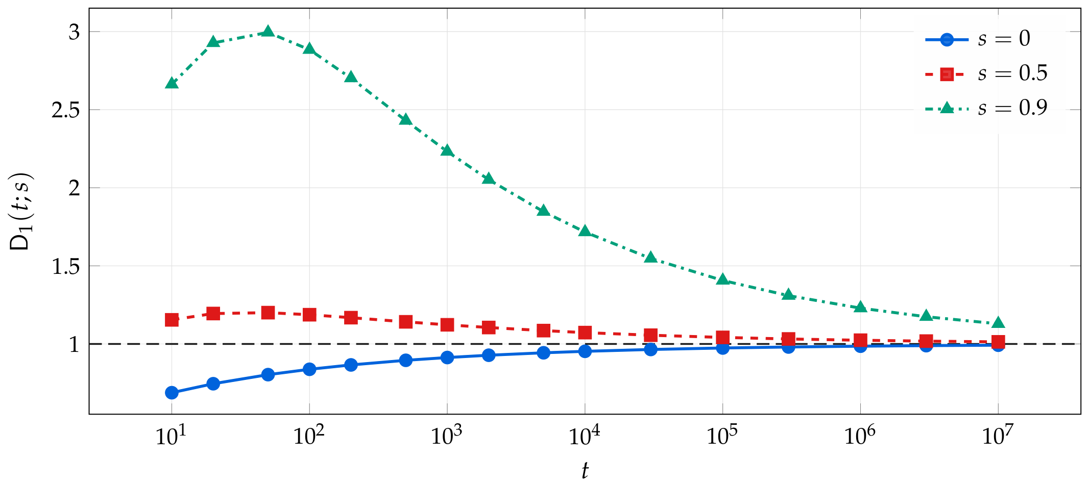
Figure 2.
Left: Model B on the boundary , the immigration intensity moved across the threshold , with ; the dark lines mark the constants and that (75) predicts at for the two rows, and each curve settles on its own to four figures. Right: Model R, with , the relative deviation divided by the leading term predicted for it in (84); it decreases monotonically to the dark line at 1, so that both the constant and the exponent are confirmed at once.
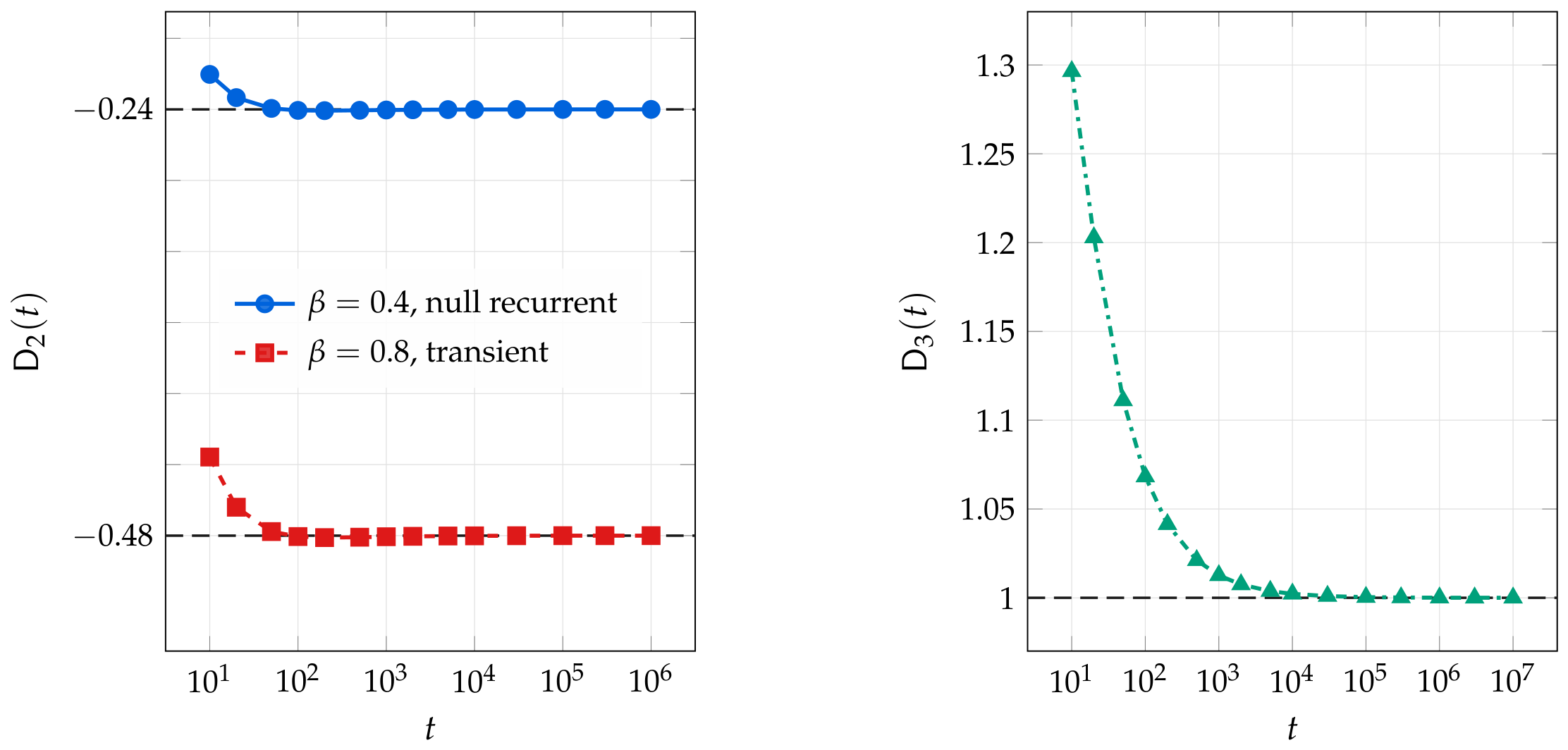

Table 1.
The four parameter sets of the family (103) and the constants (105) they produce, one for each regime of Theorem 6. All of them carry the scale and the remainder parameters , , so that , and throughout. The two rows of Model B carry one and the same branching mechanism and differ only in the immigration intensity, which is moved across the threshold of Theorem 6(ii).
| Model T | transient | ||||||||
| Model B | null recurrent | 0 | |||||||
| Model B | transient | 0 | |||||||
| Model R | positive recurrent |
Table 2.
Model T. The three-term expansion (29) of the survival probability , in the form of , against the exact value; the last column is the ratio of the two preceding ones.
Table 2.
Model T. The three-term expansion (29) of the survival probability , in the form of , against the exact value; the last column is the ratio of the two preceding ones.
| t | right-hand side of (29) | ratio | ||
|---|---|---|---|---|
Table 3.
Model T, transient regime. Left: the exact identity (70), whose second column approaches the constant of that formula. Right: the rate (71), its leading term evaluated at the exact rather than at ; the tail integral agrees with it up to the term discarded there, the last column being the ratio of the two. For Model T the coefficient happens to equal , since there.
| t | ratio | |||
|---|---|---|---|---|
Table 4.
Model T with . Left: the limits of (93), the value being forced since , and beside them the deviations of the local ratios from those limits. Right: the scaled supremum of the deviation of from on the circle . Both are defined in the text above, each divided by the order predicted for it.
Table 4.
Model T with . Left: the limits of (93), the value being forced since , and beside them the deviations of the local ratios from those limits. Right: the scaled supremum of the deviation of from on the circle . Both are defined in the text above, each divided by the order predicted for it.
| j | t | |||||
|---|---|---|---|---|---|---|
| 2 | ||||||
| 4 | ||||||
| 6 | ||||||
| 8 | ||||||
| 12 | ||||||
| 20 |
Disclaimer/Publisher’s Note: The statements, opinions and data contained in all publications are solely those of the individual author(s) and contributor(s) and not of MDPI and/or the editor(s). MDPI and/or the editor(s) disclaim responsibility for any injury to people or property resulting from any ideas, methods, instructions or products referred to in the content. |
© 2026 by the authors. Licensee MDPI, Basel, Switzerland. This article is an open access article distributed under the terms and conditions of the Creative Commons Attribution (CC BY) license (http://creativecommons.org/licenses/by/4.0/).
Copyright: This open access article is published under a Creative Commons CC BY 4.0 license, which permit the free download, distribution, and reuse, provided that the author and preprint are cited in any reuse.