

Submitted:
18 September 2026
Posted:
20 September 2026
You are already at the latest version
Abstract
This work proposes a methodology for sea level time series imputation based on separating the observed signal into an astronomical tidal component (via harmonic analysis using T-TIDE) and a residual non tidal component, which is then modeled using a multilayer perceptron (MLP) with meteorological variables (wind, pressure, sea surface temperature) from ERA5 and cyclical temporal features (sine/cosine encoding). The main contribution consists in separating the observed signal into two physically meaningful components: (i) the tidal astronomical component, obtained through classical harmonic analysis, and (ii) the residual component, which captures non tidal variability. Subsequently, the residual component is modeled using a multilayer perceptron (MLP) using meteorological variables from ERA5 and time data as the feature vector. The method is evaluated at four NOAA tide gauge stations along the California coast (San Diego, La Jolla, Los Angeles, San Francisco) from 1950 to 2025 with a temporal resolution of one hour, with missing data fractions ranging from January 1, 1950, to June 30, 2025, at hourly resolution. The harmonic-plus-MLP approach achieves a coefficient of determination (R2) of 0.9955 and a root mean square error (RMSE) of 0.03475 across the four stations, representing an average reduction of 52% in RMSE compared to classical harmonic analysis alone.
Keywords:
sea level reconstruction
; time series imputation
; harmonic analysis
; multilayer perceptron
; ERA5 reanalysis
; residual modeling
; tidal decomposition
; coastal oceanography
1. Introduction
Sea level is mainly influenced by the gravitational interaction between the Earth, Moon and Sun, which generates phenomena such as tides [1]. In addition to the astronomical component, sea level can also be modulated by atmospheric and oceanic factors, such as wind, atmospheric pressure, and the regional dynamics of currents, as well as by large scale patterns such as the El Niño Southern Oscillation (ENSO) and the Pacific Decadal Oscillation (PDO) [2]. During the 20th century, mean sea level is estimated to have risen by approximately 10 cm, and it is currently increasing at a rate of about 1–2 mm per year; this change is associated with global warming, thermal expansion, and glacier melt [3]. As a result, the risk of coastal flooding, upwelling, and shoreline erosion increases, representing a threat to the infrastructure and the safety of cities located in coastal regions [4].
Sea level time series represent an effort to collect and analyze chronologically organized information in order to understand the historical behavior of the ocean and estimate its future evolution [5]. However, missing data in these series can induce errors in the analysis, leading to inaccurate trend estimates and hindering the identification of periodic signals such as seasonal cycles or tide related components. This problem reduces the reliability of statistical models and limits the ability to generate robust projections for future scenarios [6].
The California coast has an approximate shoreline length of 5,515 km, [7] making it a region with extensive coastal exposure and pronounced sea level variability. In addition, the California coast hosts several institutions dedicated to scientific research, including the Southwest Fisheries Science Center, CalCOFI Laboratories, the California Ocean Science Trust, and the Ames Research Center. These institutions contribute to the understanding of sea level variability, marine ecosystem changes, and the development of technologies for the conservation and sustainable management of marine environments.
The present study uses sea level observations recorded by tide gauges operated by the National Oceanic and Atmospheric Administration (NOAA), considering NOAA’s international recognition as a leading authority in oceanographic observations, the high quality and consistency of its measurements, the availability of long term historical records, and the open accessibility of its data.
Different approaches can be used, for time series reconstruction, ranging from classical statistical methods to neural network based models. Among the classical methods, one of the most widely used is the autoregressive integrated moving average (ARIMA) model [8]. A more elaborate variant is the Seasonal ARIMA (SARIMA) model, which explicitly incorporates periodic components and allows a better representation of regular seasonal patterns commonly observed in time series data [5]. However, one of its main limitations is that it often assumes linear relationships between the predictor variables and the target variable. To overcome this restriction, neural network models can be implemented, as they allow more complex and nonlinear patterns present in time series dynamics to be captured [9].
Deep learning based models have become particularly relevant for time series modeling and missing data imputation, including architectures such as GRU-D [10], M-RNN [11], and BRITS [12] as well as Convolutional neural network (CNN)-based models, such as TimesNet [13] and GP-VAE [14], as well as graph neural networks (GNNs) [15]. More recently, attention-based models, including CDSA[16], Transformers [17], SAITS [18], and NRTSI [19], have demonstrated superior performance over traditional statistical approaches. Despite these advantages, such improvements often come at the cost of increased computational complexity and higher memory requirements. In contrast, multilayer perceptrons (MLPs), when combined with well designed features, provide a computationally efficient alternative while maintaining model simplicity.
An important distinction in time series modeling is that between forecasting and imputation. While forecasting estimates future values from previously available information, imputation reconstructs missing observations within an existing time series. Recurrent neural networks (RNNs) are well suited to sequential modeling but may face difficulties with long contiguous gaps due to the lack of observations within the missing interval. In contrast, the approach adopted in this study treats sea level reconstruction as an imputation problem, using an MLP to estimate the non tidal residual from meteorological and temporal predictors.
A widely used type of neural network is the multilayer perceptron (MLP), known for its application in pattern recognition. In this model, information flows only forward, from the input layer through one or more hidden layers to the output layer. During training, the model parameters (weights and biases) are adjusted using a backpropagation algorithm in order to minimize the error and produce outputs that become increasingly closer to the expected values [20]. From a theoretical perspective, MLPs are universal function approximators, meaning that they can approximate any continuous nonlinear function with arbitrary accuracy given a sufficient number of hidden units [21]. In practice, however, well designed MLP architectures often achieve competitive performance with a relatively small number of neurons, resulting in reduced computational cost during training.
Sea level can be described as the combination of two main components: the astronomical tide and the meteorological tide. The astronomical tide responds to the gravitational forcing by celestial bodies and is analyzed using the T-TIDE toolbox proposed by Pawlowicz. [22], allowing the extraction of tidal signals. On the other hand, the meteorological tide corresponds to phenomena unrelated to astronomical interactions. In this context, the main contribution of the proposed methodology consists of modeling the residual component through a multilayer perceptron (MLP), designed to predict the non tidal variability and support the reconstruction of missing data in the time series.
This paper is organized as follows: Section 3 presents the materials and methods, including sea level series data source, handling of missing and invalid data, harmonic analysis, residual determination, meteorological variables obtained from ERA5, MLP training, network architecture, training strategy, residual imputation, and model evaluation. Section 4 presents the results of the imputations for the La Jolla, Los Angeles, San Diego, and San Francisco stations, together with the statistical evaluation of the reconstructed sea level series. Section 5 discusses the results obtained. Finally, Section 6 summarizes the main conclusions and future research directions.
2. Workflow
Figure 1 presents the general workflow of the proposed methodology for sea level time series reconstruction. The process begins with the acquisition of sea level observations from NOAA tide gauge records. These data are first subjected to preprocessing, including the handling of missing or invalid values and normalization to ensure consistency for subsequent analysis. Next, harmonic analysis is applied to estimate the astronomical tidal component of the signal. Once the tidal contribution is identified, the residual component is obtained by subtracting the harmonic reconstruction from the original observations.
Afterward, meteorological variables from the ERA5 reanalysis dataset are incorporated as external predictors. These variables, together with temporal information, are used in the training stage of a multilayer perceptron (MLP) model. The trained network is then employed to estimate missing values within the residual series through a residual imputation step. Finally, the complete sea level signal is reconstructed by combining the harmonic component with the completed residual series, and the resulting time series is evaluated using statistical performance metrics.
3. Materials and Methods
3.1. Sea Level Time Series
Sea level data were obtained from tide gauge stations of the [23], while the associated atmospheric variables were extracted from the ERA5 reanalysis dataset developed by the European Centre for Medium Range Weather Forecasts (ECMWF) [24]. The experiment used sea level records from four tide gauge stations in the California Coast: San Diego, La Jolla, San Francisco, and Los Angeles. The analysis period covered January 1, 1950, to June 30, 2025 with a temporal resolution of one hour. Figure 2 shows the geographic location of the four stations considered in the study, while Table 1 summarizes the main characteristics of each dataset.
3.2. Handling of Missing and Invalidad Data
To ensure a consistent temporal structure and to properly identify missing or invalid observations, time series were preprocessed using a gap completion strategy based on an hourly time grid. First, the raw dataset was inspected to identify incomplete timestamp information. The dataset contains the fields year, month, day, hour, minute, and water level. Records with missing values in any of the timestamp fields (year, month, day, hour, or minute) were removed, as they cannot be mapped to a valid datetime index. No further preprocessing steps were required, as the dataset already met the necessary quality standards, exhibiting no redundant entries, duplicate records, or significant outliers that required correction.
After constructing the datetime index, a complete hourly sequence was generated from the earliest to the latest available timestamp. The dataset was then reindexed to this full hourly range, forcing the insertion of any missing time steps as explicit gaps. As a result, all missing observations are represented as NaN values in the water level field, while maintaining a temporally uniform sampling interval. Finally, the datetime index was converted back to separate columns (year, month, day, hour, minute) to preserve the original file structure and facilitate downstream processing.
3.3. Harmonic Analysis
In many oceanic time series, tides represent one of the most important components of sea level variability and exhibit a predominantly periodic behavior associated with astronomical forcing. Consequently, they can be modeled using classical harmonic analysis, which represents the signal as the sum of periodic waves with known frequencies, such as and , among others. Under this approach, amplitudes and phases are estimated through a least squares fitting procedure, allowing tidal signals to be reconstructed and predicted even during periods with incomplete observations. Tools such as T-TIDE implement this methodology and are widely used in oceanographic studies [22]. Once the astronomical component has been removed, the residual signal can be modeled using meteorological predictors in order to capture non tidal variability.
Therefore, the proposed methodology separates the observed sea level into an astronomical component and a residual component . The astronomical component is estimated through classical harmonic analysis, in which the tide is represented as a finite sum of cosine functions with known frequencies. In particular, the astronomical tide can be expressed as:
where denotes the mean sea level, while and represent the amplitude and phase lag of the i-th tidal constituent, respectively. Here, corresponds to the angular frequency associated with each tidal constituent (e.g., , , , and ), and N is the total number of constituents considered [25].
Harmonic tidal analysis is a conventional approach in oceanography [22] and is widely used by operational tidal services to reconstruct and predict the astronomical tidal component [26]. In this study, this harmonic only reconstruction is therefore considered as a reference approach, while the proposed methodology extends it by incorporating the meteorologically driven non tidal residual.
3.4. Residual Determination
Once the astronomical component was reconstructed for each temporal window, the residual signal was obtained as the difference between the observed sea level and the synthesized tidal component:
The residual represents the non astronomical contribution to sea level variability. Because the harmonic reconstruction preserves only strictly periodic components, the residual retains low frequency meteorological signals, instrumental biases, and other unknown contributions that may be either stochastic or deterministic. This separation allows the modeling framework to focus exclusively on the physically meaningful non tidal variability using atmospheric features from ERA5.
3.5. Meteorological Variables (ERA5)
Meteorological features were obtained from the ERA5 reanalysis produced by the Copernicus Climate Change Service (C3S) and accessed through the Climate Data Store (CDS) API. Data were retrieved from the dataset reanalysis era5 single levels, which provides hourly global reanalysis fields at the surface and near surface level.
For each tide gauge location, ERA5 variables were extracted over a rectangular spatial domain defined by latitude–longitude bounds in the CDS “area” format [N, W, S, E]. The bounding box was selected to represent local atmospheric and oceanic forcing conditions near the station.
The following physical variables were downloaded with hourly resolution:
- East-West wind component in meters per second [m/s] at a height of ten meters above the surface of the Earth
- North-South wind component in meters per second [m/s] at a height of ten meters above the surface of the Earth
- Mean sea level atmospheric pressure adjusted to the height of mean sea level in [Pa]
- Sea surface temperature near the surface in [K]
- Sea surface atmospheric pressure at the surface of land, sea and inland water in [Pa]
Data were obtained as monthly NetCDF files using a year month loop. Each request included all calendar days and the 24 hourly time stamps (00–23), allowing CDS to return the valid subset for each month.
3.6. MLP Training
3.6.1. Meteorological Features (ERA5)
In the temporal dimension, ERA5 variables were retrieved at hourly resolution and synchronized with the corresponding sea level observations.
where represents the meteorological forcing vector used as input to the neural network.
3.6.2. Cyclical Temporal Variables (Sine/Cosine)
To avoid artificial discontinuities (for example, between 23:00 and 00:00, or between December and January), time variables are transformed into a cyclical representation using sine/cosine pairs. In particular, the following vector is constructed:
where , , , and represent the angular transformations associated with the year (Y), month (M), day (D), and hour (H), respectively. Each temporal variable is encoded through its sine and cosine components, and , enabling a continuous representation of cyclical temporal patterns. Finally [27]. The complete input vector is defined as:
3.7. Network Architecture
The complete input vector is provided to a fully connected feed forward artificial neural network, known as a multilayer perceptron (MLP) with three hidden layers. The architecture is defined by a hyperparameter vector , where denotes the number of neurons in the i-th hidden layer. In the present implementation, the network configuration was set to . Hidden layers employed the hyperbolic tangent sigmoid activation function (tansig), while the output layer used a linear activation function (purelin). The overall architecture of the network is illustrated in Figure 3.
3.8. Training Strategy
The network was implemented using MATLAB’s Neural Network Toolbox.Physical predictors were normalized to the range , while temporal variables were encoded using sine cosine transformations to ensure a smooth cyclical representation. 70% of available residual samples were used for training, 15% for validation (early stopping) and 15% for cross validation, implementing the dividetrain method. The loss function was defined as the mean squared error (MSE).
Model optimization was carried out using the scaled conjugate gradient (SCG) algorithm. The training process was configured with a maximum of 1000 epochs, a minimum gradient threshold of . To prevent overfitting, early stopping was applied: training was halted when the validation loss did not improve for 10 consecutive epochs, and the best-performing model parameters were restored.
For the reconstruction of missing values, the MLP model was applied using sliding temporal windows of five years. These windows were selected based on the presence of gaps in the time series, ensuring that each training segment contains sufficient valid data to learn the underlying patterns. Within each window, the model was trained and subsequently used to predict the missing values corresponding to that specific period.
3.9. Residual Imputation
Once the network parameters were optimized using valid residual observations, the trained model was applied to the complete input dataset in order to estimate missing residual values. Let denote the observed residual component and the MLP prediction used for time steps where is unavailable. The reconstructed residual series, , is defined as:
3.10. Time Series Reconstruction
Once the residual component was completed through the imputation procedure, the full sea level time series was reconstructed by combining the harmonic prediction with the residual signal. Let denote the harmonic component obtained from the classical tidal analysis and the reconstructed residual series. The reconstructed sea level signal, , is then obtained as
When observed residual values are available, the reconstruction uses the original residual component. Otherwise, the missing residuals are replaced by the MLP based imputation.
3.11. Model Evaluation
Model performance was evaluated in two phases, first predicting already known data and evaluating the coefficient of determination () and the root mean squared error (RMSE). The coefficient of determination is defined as:
where denotes the observed residual, the predicted residual, and the mean of the observed residual series. The coefficient quantifies the proportion of residual variance explained by the network model. The RMSE was computed as:
The RMSE measures the average magnitude of the deviation between predicted and observed residuals.
Additionally, to assess whether the imputation preserves the fundamental statistical properties of the time series, descriptive statistics were compared between the observed and imputed data: The mean of the original residual series () was compared with the mean of the imputed residual series () in order to evaluate the preservation of central tendency. Similarly, the variance of the original series () was contrasted with that of the imputed series () to assess consistency in variability.
Beyond central tendency and dispersion measures, statistics including skewness and kurtosis were analyzed following the same approach. The skewness of the original residual series () was compared with that of the imputed series () to determine whether distributional asymmetry was preserved. Also, the kurtosis of the original series () was evaluated against the kurtosis of the imputed series () to verify the maintenance of tail behavior after reconstruction.
4. Results
4.1. Residual Imputation
A set of residual imputation results examples, for the selected stations, are shown in Figure 4, Figure 5, Figure 6 and Figure 7, where missing intervals are replaced using the corresponding MLP based estimates. Missing intervals are replaced using the corresponding MLP based estimates.
A summary of the statistical metrics comparing the observed residual series and the MLP based imputed values for the La Jolla, Los Angeles, San Diego and San Francisco stations are presented in Table 2, Table 3, Table 4 and Table 5.
The performance of the proposed MLP based imputed residuals was assessed using residual sea level records from the La Jolla, Los Angeles, San Diego, and San Francisco stations. A comparison between the observed and reconstructed residual series revealed that the reconstructed data consistently reproduced the overall statistical behavior of the original records, including their mean, variance, skewness, and kurtosis. The mean values of the reconstructed residuals remained close to zero and were consistent with those of the observed residuals, as expected from the centering of the residual series during preprocessing, indicating preservation of the central tendency. Likewise, the reconstructed residuals retained variance values of the same order of magnitude as the observed series, demonstrating preservation of the main dispersion characteristics of the residual data. With respect to reconstruction accuracy, all study cases yielded coefficients of determination greater than 0.60, with the highest values exceeding 0.85, while RMSE values remained below 0.055 m across all experiments.
4.2. Statistical Evaluation of the Reconstructed Sea Level Series
A statistical comparison between the observed sea level series and the reconstructed sea level series was performed for the four tide gauge stations. Table 6 presents the corresponding statistics for the classical harmonic analysis, while Table 7 summarizes the main statistical metrics used to evaluate the reconstruction performance, and Table 8 presents the main statistical metrics used to evaluate the reconstruction performance. For each station, the reported corresponds to the mean coefficient of determination obtained from the different reconstruction windows evaluated. Overall, the inclusion of the residual model reduced the RMSE by approximately 52% across the four stations.
To better highlight the improvement obtained by the MLP model with harmonics imputed residual values relative to the classical harmonic values, Table 8 presents the differences in performance metrics.
The MLP with residual reconstruction shows a significant improvement over the classical harmonic approach. As shown in Tables 6–8, the proposed method increases from an average of 0.9794 to 0.9955 across the four stations, while reducing the RMSE from an average of 0.0743 to 0.0348. This represents an average RMSE reduction of 53%, indicating that the MLP with residual imputation substantially improves the reconstruction accuracy of the sea level series despite the limitations imposed by the fixed training window.
5. Discussion
The combination of the astronomical tide with the imputed residual with meteorological variables produces an highly accurate reconstruction of the observed sea level series. The coefficients of determination for all the complete series between 1 January 1950 to 30 June 2025 are close to 0.995 at all stations (Table 7), quantifying the gain obtained by incorporating the residual modeling.
The proposed model obtains a clear improvement in predictive performance in comparison with other approaches reported in the literature, such as the feedforward model proposed by [28], which reports values from 0.8318 to 0.8775 and RMSE values between 0.059 and 0.079. Similar results are observed when comparing the proposed approach with several models reported by [29], including Prophet, LSTM, and GRU. These models report performance values of approximately 0.71 to 0.95 and RMSE values around 0.054 to 0.023.
These comparisons should consider the distinction between forecasting and imputation. Although recurrent models such as LSTM and GRU effectively capture temporal dependencies, their performance may decrease when imputing long contiguous gaps due to error propagation from sequential estimates. In contrast, the proposed MLP estimates the non tidal residual from meteorological and temporal predictors without relying on previous reconstructed values, making it suitable for contiguous missing intervals.
A critical aspect in data imputation is preserving the fundamental statistical properties of the time series. The comparative analysis of the mean, variance, skewness, and kurtosis between the observed and imputed residuals reveals important findings.
The mean of the imputed residuals is practically identical to that of the observed residuals in all cases, demonstrating that the model is essentially unbiased. However, it is consistently observed that the variance of the imputed residuals is lower than that of the observed residuals. This behavior is typical of regression based models, which tend to predict toward the conditional mean and therefore do not fully capture the complete high frequency variability present in the original series. As a result, the imputed residuals exhibit a slight reduction in variance compared to the observed residuals. This tendency has been widely documented in predictive modeling and data imputation contexts [30].
The preservation of higher order statistical moments shows more variable behavior. In general, the model correctly captures the direction of the skewness observed in the residual series; however, its magnitude is often slightly amplified in the imputed data.
Despite the promising results obtained in this study, several limitations should be acknowledged. First, the training strategy based on fixed five year windows may limit the model’s ability to capture long term climatic variability and regime shifts that occur at larger temporal scales. Second, the proposed approach was evaluated using a limited number of tide gauge stations, which may restrict the generalizability of the results to other coastal regions with different oceanographic conditions.
Although these limitations, the proposed framework offers a scalable and physically consistent solution for large scale sea level reconstruction and missing data imputation across diverse coastal environments, particularly due to its reliance on freely available data sources such as NOAA and ERA5.
Finally, the model shows a strong dependence on the combined use of meteorological and cyclical variables, since removing either component reduces the predictive accuracy by approximately 40%. Future research should explore adaptive training windows, the incorporation of additional physical predictors, and the evaluation of the method across a broader network of tide gauge stations.
6. Conclusions
The results obtained in this study strongly suggest that the proposed methodology provides an effective framework for reconstructing incomplete sea level time series. the method captures both the deterministic tidal signal and the tidal variability by combining harmonic analysis with a multilayer perceptron model applied to the residual component. Overall, the proposed approach shows clear performance advantages over traditional methods reported in the literature.
The use of freely available and highly reliable data sources such as NOAA and ERA5 is a strong point of the proposed methodology since it improves the reproducibility of the experimental portion of this work and its possible use over different oceanic regions.
Author Contributions
SALR developed the methodology, implemented the main software framework, and performed the data analysis. LTF supervised this work. JAMV developed the modelohibrido.m script. JAMV, MACL, and ICL contributed to the conceptualization and design of the study, the interpretation of the data, and the preparation of the article.
Funding
This research received no external funding.
Institutional Review Board Statement
Not applicable.
Informed Consent Statement
Not applicable.
Data Availability Statement
Sea level data are available from NOAA tide gauges, and meteorological variables are available from the ERA5 reanalysis dataset.The source code used in this study is publicly available at https://doi.org/10.5281/zenodo.21381831.
Conflicts of Interest
The authors declare no conflicts of interest.
References
- Hartmann, D.L. Global Physical Climatology; Academic Press: San Diego, CA, USA, 1994. [Google Scholar]
- Grossman, E.E.; Tehranirad, B.; Nederhoff, C.M.; Crosby, S.C.; Stevens, A.W.; Van Arendonk, N.R.; Nowacki, D.J.; Erikson, L.H.; Barnard, P.L. Modeling Extreme Water Levels in the Salish Sea: The Importance of Including Remote Sea Level Anomalies for Application in Hydrodynamic Simulations. Water 2023, 15, 4167. [Google Scholar] [CrossRef]
- National Research Council. Sea-Level Rise for the Coasts of California, Oregon, and Washington: Past, Present, and Future; The National Academies Press: Washington, DC, USA, 2012. [Google Scholar] [CrossRef] [PubMed]
- Webb, P. Introduction to Oceanography; Open Educational Resource, 2018. [Google Scholar]
- Nielsen, A. Practical Time Series Analysis: Prediction with Statistics & Machine Learning; O’Reilly Media: Sebastopol, CA, USA, 2020. [Google Scholar]
- Chakraborty, S.; Ide, K.; Balachandran, B. Missing values imputation in ocean buoy time series data. Ocean Eng. 2025, 318, 120145. [Google Scholar] [CrossRef]
- NOAA Office for Coastal Management. Shoreline Mileage of the United States (PDF). 2026. Available online: https://coast.noaa.gov/data/docs/states/shorelines.pdf (accessed on Jan. 25 2026).
- Géron, A. Hands-On Machine Learning with Scikit-Learn, Keras & TensorFlow: Concepts, Tools, and Techniques to Build Intelligent Systems, 2 ed.; O’Reilly Media: Sebastopol, CA, USA, 2019. [Google Scholar]
- Tetko, I.V.; Kůrková, V.; Karpov, P.; Theis, F. (Eds.) Artificial Neural Networks and Machine Learning – ICANN 2019: Text and Time Series . In Lecture Notes in Computer Science (LNCS) Proceedings of ICANN 2019; Munich, Germany, Springer: Cham, Switzerland, 2019; Vol. 11730. [Google Scholar]
- Che, Z.; Purushotham, S.; Cho, K.; Sontag, D.; Liu, Y. Recurrent Neural Networks for Multivariate Time Series with Missing Values. Sci. Rep. 2018, 8, 6085. [Google Scholar] [CrossRef] [PubMed]
- Yoon, J.; Zame, W.R.; van der Schaar, M. Estimating Missing Data in Temporal Data Streams Using Multi-directional Recurrent Neural Networks. IEEE Trans. Biomed. Eng. 2019, 66, 1477–1490. [Google Scholar] [CrossRef] [PubMed]
- Cao, W.; Wang, D.; Li, J.; Zhou, H.; Li, L.; Li, Y. BRITS: Bidirectional Recurrent Imputation for Time Series. Proc. Adv. Neural Inf. Process. Syst. 2018, Vol. 31, 6775–6785. [Google Scholar]
- Wu, H.; Yin, J.; Long, M.; Wang, J. TimesNet: Temporal 2D-Variation Modeling for General Time Series Analysis. In Proceedings of the Proceedings of the International Conference on Learning Representations (ICLR), 2023. [Google Scholar]
- Fortuin, V.; Baranchuk, D.; Rätsch, G.; Mandt, S. GP-VAE: Deep Probabilistic Time Series Imputation. In Proceedings of the Proceedings of the International Conference on Artificial Intelligence and Statistics (AISTATS), 2020. [Google Scholar]
- Cini, A.; Marisca, I.; Alippi, C. Filling the Gaps: Multivariate Time Series Imputation by Graph Neural Networks. In Proceedings of the Proceedings of the International Conference on Learning Representations (ICLR), Virtual Conference Published as a conference paper at ICLR 2022, 2022. [Google Scholar]
- Ma, J.; Shou, Z.; Zareian, A.; Vetro, A.; Mansour, H. CDSA: Cross-Dimensional Self-Attention for Multivariate, Geo-tagged Time Series Imputation. arXiv 2019, arXiv:1905.04074. [Google Scholar]
- Vaswani, A.; Shazeer, N.; Parmar, N.; Uszkoreit, J.; Jones, L.; Gomez, A.N.; Kaiser; Polosukhin, I. Attention Is All You Need. In Proceedings of the Advances in Neural Information Processing Systems; Curran Associates, Inc., 2017; Vol. 30. [Google Scholar]
- Du, W.; Cote, D.; Liu, Y. SAITS: Self-Attention-Based Imputation for Time Series. Expert Syst. With Appl. 2023, 219, 119619. [Google Scholar] [CrossRef]
- Shan, S.; Li, Y.; Qin, J. NRTSI: Non-Recurrent Time Series Imputation. arXiv 2021, arXiv:2102.03340. [Google Scholar]
- Zhai, M.; Cao, Q.; Huo, P.; Du, X.; Xin, M. Estuary-Tidal Residual Water Level Forecasting Method Based on Variational Mode Decomposition and Back Propagation Neural Network. J. Mar. Sci. Eng. 2025, 13, 1755. [Google Scholar] [CrossRef]
- Cybenko, G. Approximation by Superpositions of a Sigmoidal Function. Math. Control Signals Syst. 1989, 2, 303–314. [Google Scholar] [CrossRef]
- Pawlowicz, R.; Beardsley, B.; Lentz, S. Classical tidal harmonic analysis including error estimates in MATLAB using T_TIDE. Comput. Geosci. 2002, 28, 929–937. [Google Scholar] [CrossRef]
- National Oceanic and Atmospheric Administration. Tide gauge sea level data. 2026. Available online: https://tidesandcurrents.noaa.gov/ (accessed on Feb. 26 2026).
- Copernicus Climate Change Service (C3S). ERA5 single levels. Available online: https://cds.climate.copernicus.eu/datasets/reanalysis-era5-single-levels?tab=overview (accessed on Nov. 16 2025).
- Boesch, A.; Müller-Navarra, S. Reassessment of long-period constituents for tidal predictions along the German North Sea coast and its tidally influenced rivers. Ocean Sci. 2019, 15, 1363–1379. [Google Scholar] [CrossRef]
- National Oceanic and Atmospheric Harmonic. What are Harmonic Constituents. 2026. Available online: https://tidesandcurrents.noaa.gov/about_harmonic_constituents.html (accessed on Aug. 18 2026).
- Bansal, A.; Balaji, K.; Lalani, Z. Temporal Encoding Strategies for Energy Time Series Prediction. arXiv 2025, arXiv:2503.15456. [Google Scholar]
- Lee, E.J.; Kim, K.; Park, J.H. Reconstruction of long-term sea-level data gaps of tide gauge records using a neural network operator. Front. Mar. Sci. 2022, 9, 1037697. [Google Scholar] [CrossRef]
- Han, M.; Lim, H.S. Reconstructing Sea Level Variability at the Ieodo Ocean Research Station (1993–2023) Using Artificial Intelligence, Machine Learning, and Reanalysis Integration. In Earth System Science Data Discussions; 2025; Volume Preprint. [Google Scholar] [CrossRef]
- Zhang, Z. Missing data imputation: focusing on single imputation. Ann. Transl. Med. 2016, 4, 9. [Google Scholar] [CrossRef] [PubMed]
Figure 1.
Workflow of the proposed methodology for sea level time series reconstruction.
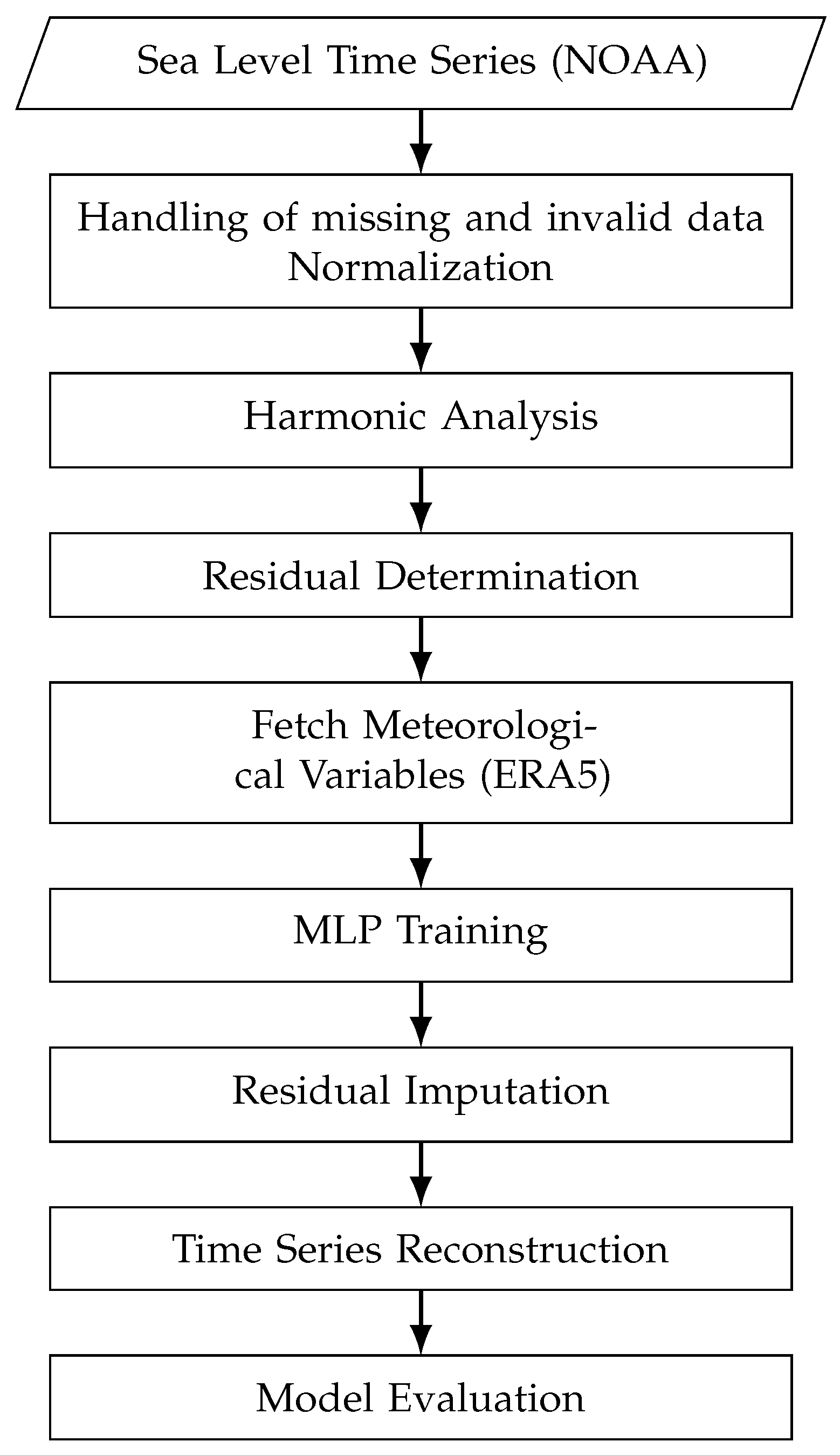
Figure 2.
Location of the tide gauges used in this study. La Jolla (Station ID: 9410230) is located at N, W. The available record spans from 1 January 1950 to 30 June 2025, with 2.83 % missing data. Los Angeles (Station ID: 9410660) is located at N, W. The available record spans from 1 January 1950 to 30 June 2025, with 0.99 % missing data. San Diego (Station ID: 9410170) is located at N, W. The available record spans from 1 January 1950 to 30 June 2025, with 1.01 % missing data. San Francisco (Station ID: 9414290) is located at N, W. The available record spans from 1 January 1950 to 30 June 2025, with 1.31 % missing data. The map was created by the authors using QGIS with Google Satellite imagery as the basemap. Basemap imagery © Google and its data providers.
Figure 2.
Location of the tide gauges used in this study. La Jolla (Station ID: 9410230) is located at N, W. The available record spans from 1 January 1950 to 30 June 2025, with 2.83 % missing data. Los Angeles (Station ID: 9410660) is located at N, W. The available record spans from 1 January 1950 to 30 June 2025, with 0.99 % missing data. San Diego (Station ID: 9410170) is located at N, W. The available record spans from 1 January 1950 to 30 June 2025, with 1.01 % missing data. San Francisco (Station ID: 9414290) is located at N, W. The available record spans from 1 January 1950 to 30 June 2025, with 1.31 % missing data. The map was created by the authors using QGIS with Google Satellite imagery as the basemap. Basemap imagery © Google and its data providers.
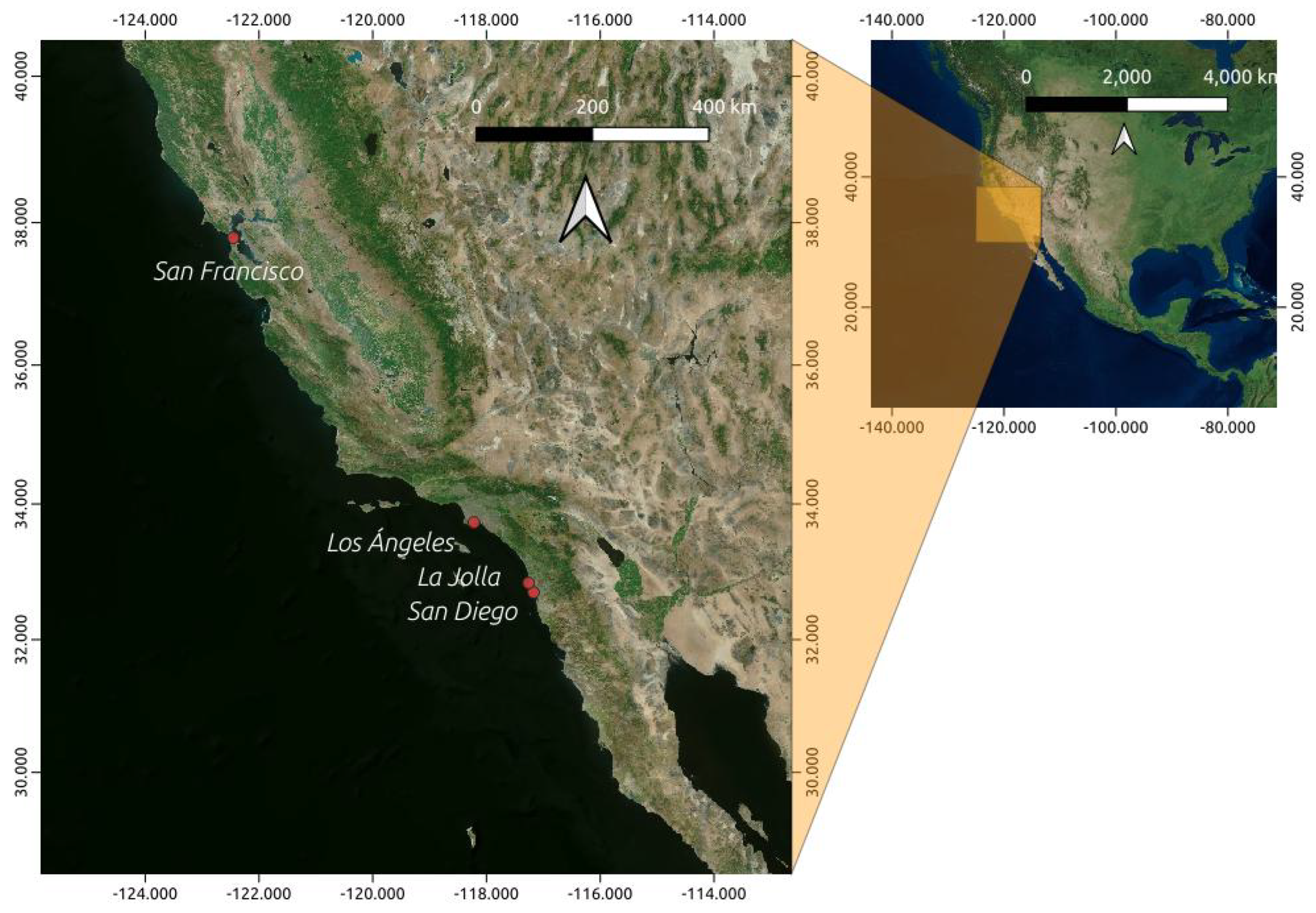
Figure 3.
Feedforward neural network architecture with three hidden layers for residual sea level modeling.
Figure 3.
Feedforward neural network architecture with three hidden layers for residual sea level modeling.
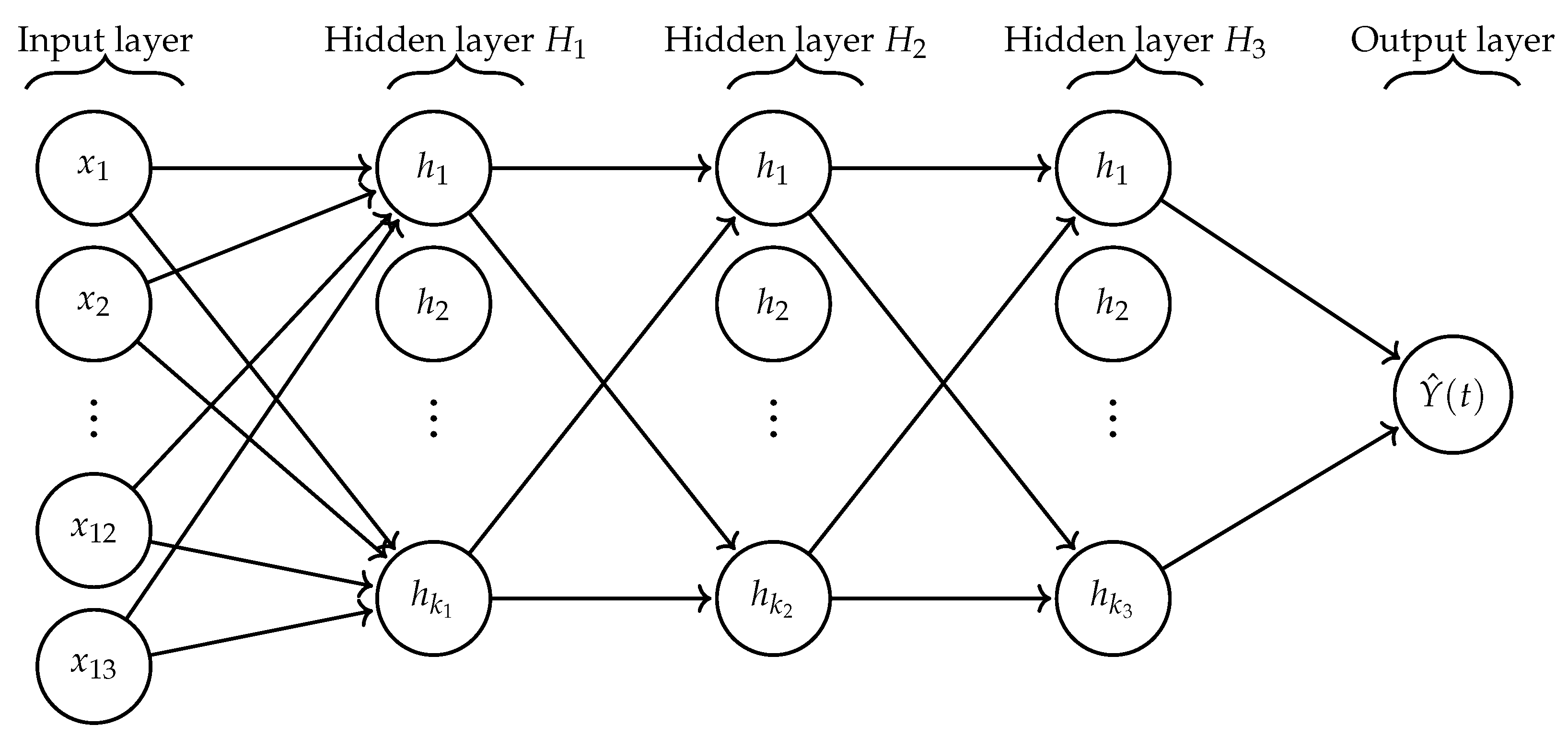
Figure 4.
Residual imputation results for La Jolla (1950–1955).
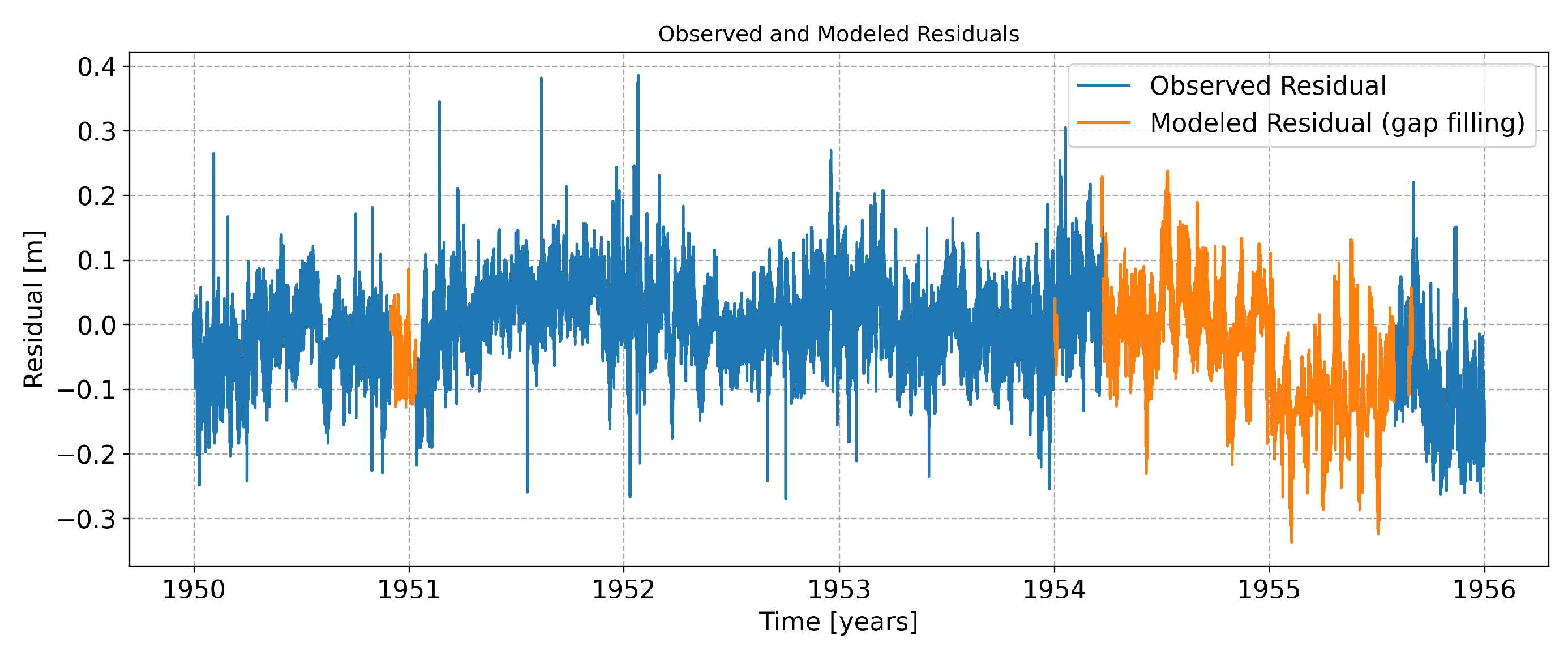
Figure 5.
Residual imputation results for Los Angeles (1975–1980).
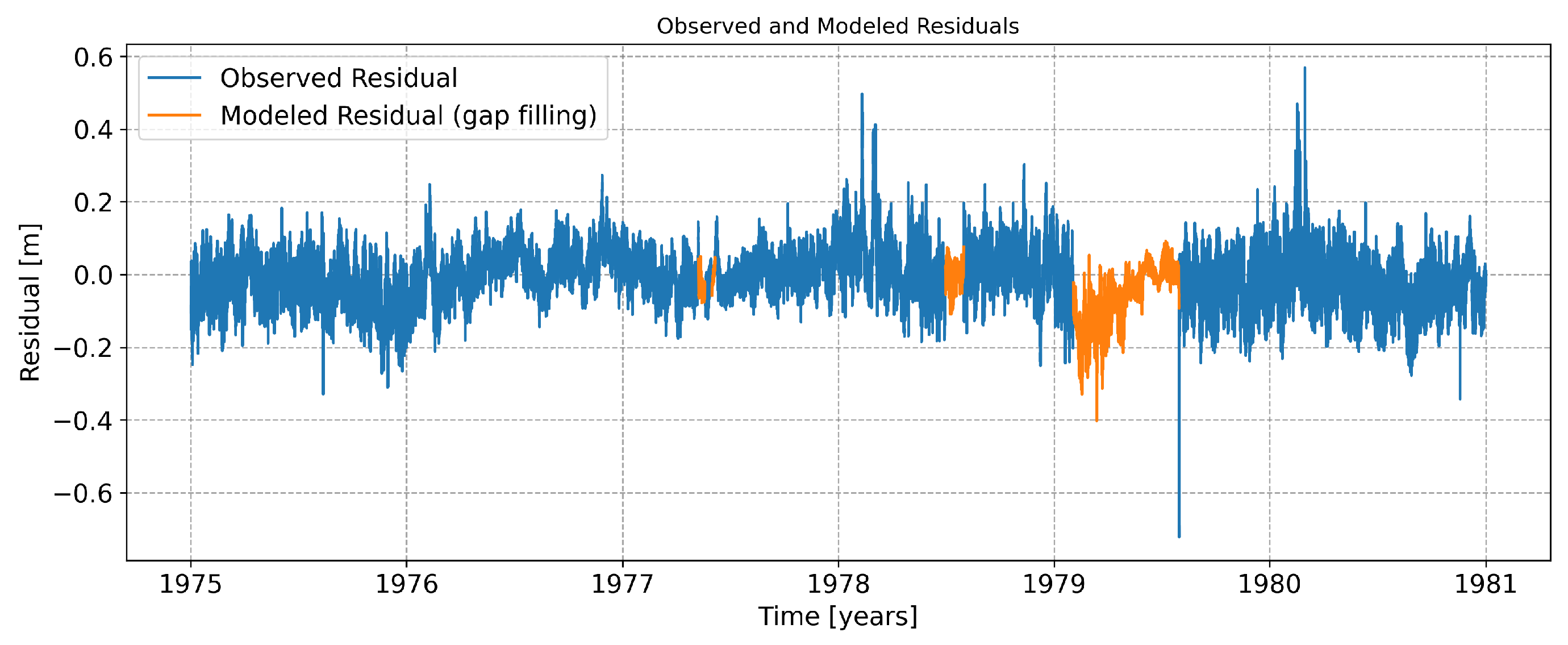
Figure 6.
Residual imputation results for San Diego (1961–1966).
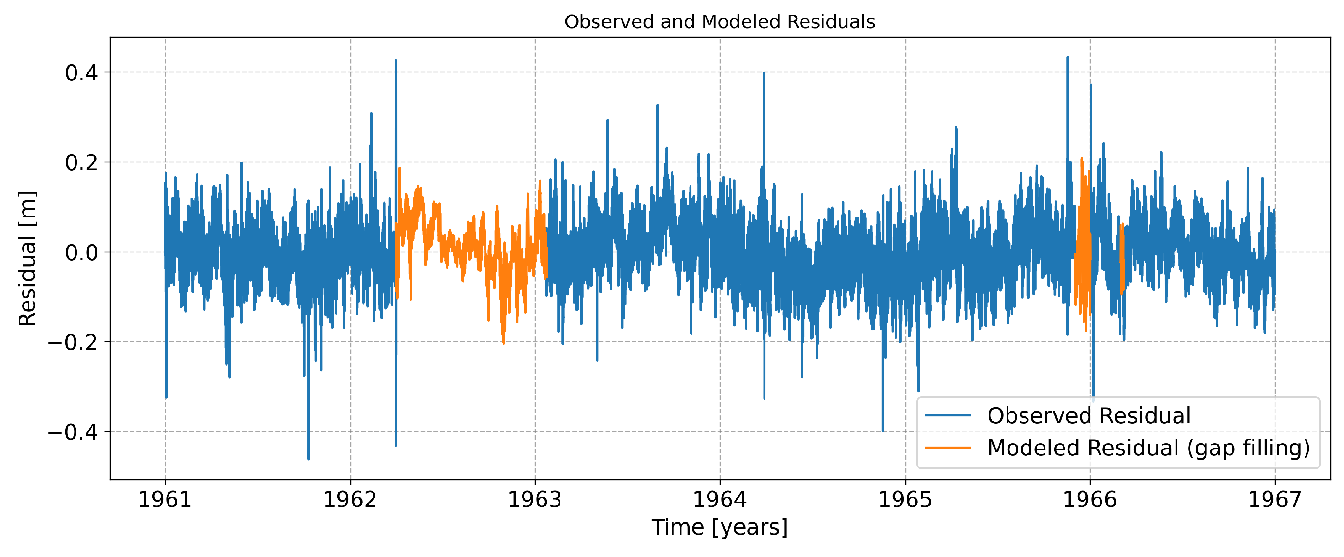
Figure 7.
Residual imputation results for San Francisco (1968–1973).
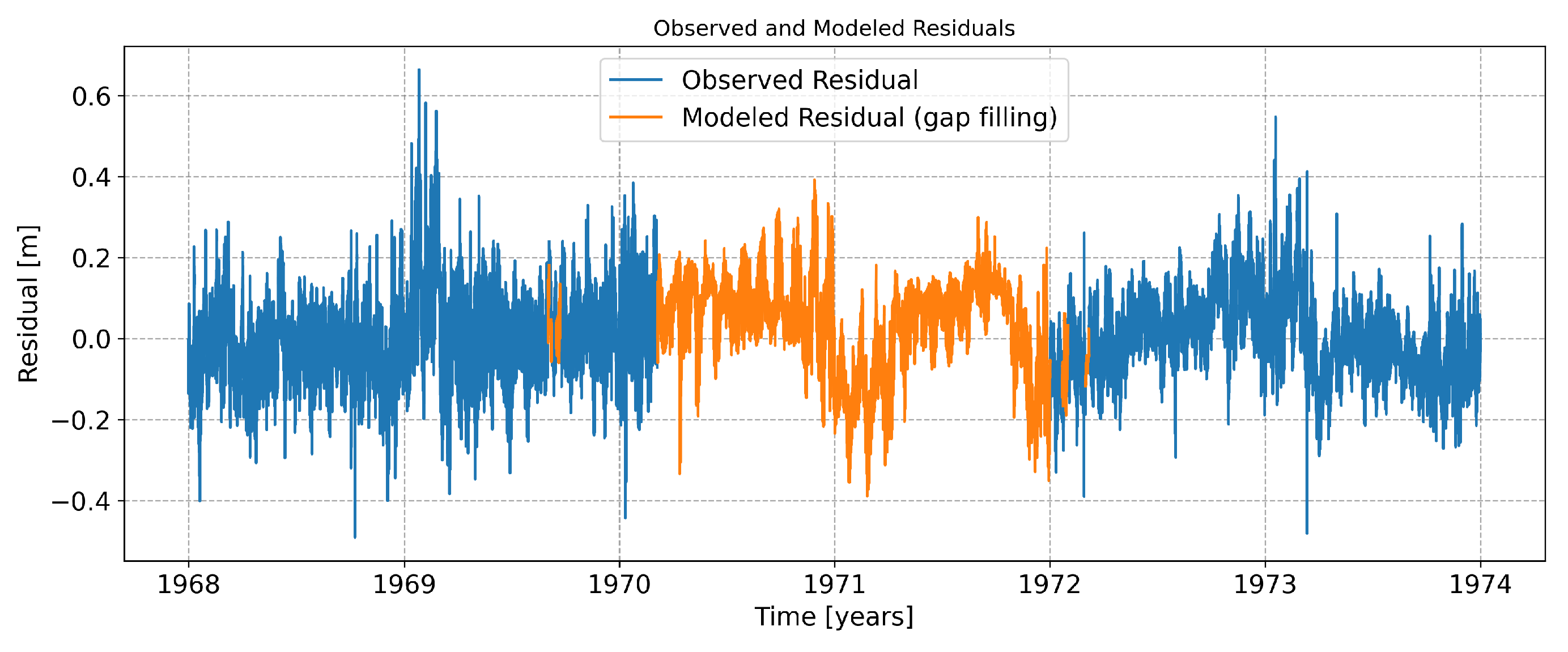

Table 1.
Summary of tide gauge stations used in this study.
| Variable | La Jolla | Los Angeles | San Diego | San Francisco |
|---|---|---|---|---|
| Latitude | N | N | N | N |
| Longitude | W | W | W | W |
| Starting date | 1950-01-01 | 1950-01-01 | 1950-01-01 | 1950-01-01 |
| Ending date | 2025-06-30 | 2025-06-30 | 2025-06-30 | 2025-06-30 |
| Available data | 653 156 | 661 072 | 654 501 | 645 818 |
| Missing data | 2.83% | 0.99% | 1.01% | 1.31% |
| Minimum | 0.559 m | 0.415 m | 0.335 m | 1.066 m |
| Maximum | 3.707 m | 3.557 m | 3.663 m | 4.511 m |
Table 2.
La Jolla station.
| Metrics | 1950-1955 | 1968-1973 | 1975-1980 |
|---|---|---|---|
| Imputed data % | 25.11% | 16.27% | 6.89% |
| 0.8281 | 0.7356 | 0.8077 | |
| RMSE | 0.028327 | 0.035394 | 0.028811 |
| Mean | -0.000003 | -0.000001 | 0.000002 |
| Imputed mean | -0.000004 | 0.000000 | 0.000001 |
| Variance | 0.000526 | 0.001105 | 0.000673 |
| Imputed variance | 0.000085 | 0.000074 | 0.000088 |
| Skewness | -0.313345 | 0.331097 | 0.091578 |
| Imputed skewness | -0.441458 | 0.472368 | 0.133955 |
| Kurtosis | 3.560449 | 4.096827 | 3.609488 |
| Imputed kurtosis | 3.439115 | 4.219871 | 3.971500 |
Table 3.
Los Angeles station.
| Metrics | 1962-1967 | 1968-1973 | 1975-1980 |
|---|---|---|---|
| Imputed data % | 2.16% | 1.24% | 10.38% |
| 0.6346 | 0.7463 | 0.6839 | |
| RMSE | 0.035276 | 0.034102 | 0.040083 |
| Mean | -0.000001 | 0.000000 | 0.000001 |
| Imputed mean | -0.000001 | 0.000001 | 0.000002 |
| Variance | 0.000857 | 0.000896 | 0.001356 |
| Imputed variance | 0.000050 | 0.000060 | 0.000063 |
| Skewness | 0.015105 | 0.137613 | 0.171657 |
| Imputed skewness | 0.113221 | 0.265876 | 0.362051 |
| Kurtosis | 4.399650 | 3.915291 | 5.079241 |
| Imputed kurtosis | 3.896616 | 3.695929 | 5.774328 |
Table 4.
San Diego station.
| Metrics | 1961-1966 | 1968-1973 | 1974-1979 | 1983-1988 |
|---|---|---|---|---|
| Imputed data % | 15.27% | 3.00% | 2.49% | 4.81% |
| 0.7190 | 0.6241 | 0.6545 | 0.8341 | |
| RMSE | 0.032080 | 0.043570 | 0.039420 | 0.027745 |
| Mean | -0.000002 | -0.000000 | -0.000000 | -0.000003 |
| Imputed mean | -0.000002 | -0.000001 | -0.000001 | -0.000002 |
| Variance | 0.000832 | 0.001043 | 0.000854 | 0.000527 |
| Imputed variance | 0.000074 | 0.000056 | 0.000075 | 0.000051 |
| Skewness | 0.048577 | 0.363637 | -0.163280 | 0.359211 |
| Imputed skewness | 0.152613 | 0.612316 | 0.112448 | 0.449569 |
| Kurtosis | 4.073231 | 4.680371 | 6.273201 | 3.954933 |
| Imputed kurtosis | 3.195088 | 4.490868 | 4.336685 | 4.280038 |
Table 5.
San Francisco station.
| Metrics | 1962-1967 | 1968-1973 | 1978-1983 | 2019-2024 |
|---|---|---|---|---|
| Imputed data % | 1.27% | 31.52% | 2.69% | 9.40% |
| 0.6339 | 0.7927 | 0.8599 | 0.8505 | |
| RMSE | 0.054210 | 0.045269 | 0.042291 | 0.032815 |
| Mean | 0.000001 | -0.000001 | -0.000002 | 0.000001 |
| Imputed mean | -0.000000 | 0.000003 | -0.000002 | -0.000001 |
| Variance | 0.001339 | 0.001439 | 0.000914 | 0.000493 |
| Imputed variance | 0.000110 | 0.000223 | 0.000126 | 0.000092 |
| Skewness | 0.411140 | 0.515945 | 0.763674 | 0.861783 |
| Imputed skewness | 0.710221 | 0.754487 | 0.866907 | 1.001570 |
| Kurtosis | 6.090925 | 4.403974 | 4.601481 | 5.242480 |
| Imputed kurtosis | 6.867007 | 5.053964 | 4.818073 | 5.632445 |
Table 6.
Summary of metrics between the sea level observed series and the classic harmonic values.
| Metrics | La Jolla | Los Angeles | San Diego | San Francisco |
|---|---|---|---|---|
| 0.9804 | 0.9830 | 0.9828 | 0.9714 | |
| RMSE | 0.0694 | 0.0661 | 0.0693 | 0.0922 |
Table 7.
Summary of metrics between the sea level observed series and the MLP based imputed residual values.
Table 7.
Summary of metrics between the sea level observed series and the MLP based imputed residual values.
| Metrics | La Jolla | Los Angeles | San Diego | San Francisco |
|---|---|---|---|---|
| 0.9959 | 0.9955 | 0.9958 | 0.9947 | |
| RMSE | 0.0315 | 0.0339 | 0.0339 | 0.0397 |
Table 8.
Variation between the classical harmonic model and the MLP with harmonics model.
| Metrics | La Jolla | Los Angeles | San Diego | San Francisco |
|---|---|---|---|---|
| 0.0158 | 0.0127 | 0.0132 | 0.0239 | |
| RMSE | -54% | -48% | -51% | -56% |
Disclaimer/Publisher’s Note: The statements, opinions and data contained in all publications are solely those of the individual author(s) and contributor(s) and not of MDPI and/or the editor(s). MDPI and/or the editor(s) disclaim responsibility for any injury to people or property resulting from any ideas, methods, instructions or products referred to in the content. |
© 2026 by the authors. Licensee MDPI, Basel, Switzerland. This article is an open access article distributed under the terms and conditions of the Creative Commons Attribution (CC BY) license (http://creativecommons.org/licenses/by/4.0/).
Copyright: This open access article is published under a Creative Commons CC BY 4.0 license, which permit the free download, distribution, and reuse, provided that the author and preprint are cited in any reuse.