

Submitted:
18 September 2026
Posted:
20 September 2026
You are already at the latest version
Abstract
In this paper we examine the relative influence of structure learning algorithms and scoring functions in Bayesian networks for healthcare applications. We compare Hill Climbing, Tabu Search, and Greedy Equivalence Search (GES) using the Bayesian Information Criterion (BIC), Bayesian Dirichlet equivalent uniform (BDeu), and K2 scoring functions on three healthcare datasets. On the full data, all three algorithms produced almost identical structures under BIC (Structural Hamming Distance [SHD] = 0 or 1). Bootstrap results showed a different pattern: Hill Climbing and Tabu Search remained identical in almost all resamples (median SHD = 0.0), whereas GES differed more from both (median SHD = 3.0–7.0). Changing the scoring function substantially altered the structure in two datasets but not the third. Overall, scoring functions produced larger differences than algorithms (median SHD = 8.5 vs. 3.0), although these values combine bootstrap and full-sample comparisons. Checks using different redundancy weights and discretization levels did not change the main pattern. Scoring functions were generally the larger source of disagreement, while algorithm agreement was less stable under resampling. Further datasets are needed to assess whether these findings generalize.
Keywords:
bayesian networks
; structure learning
; hill climbing
; tabu search
; greedy equivalence search
; healthcare data
1. Introduction
Clinical decision making increasingly relies on data driven models, yet the models that perform best on held out accuracy are often the hardest to explain to a physician who must justify a diagnosis. Bayesian networks remain attractive for this reason: a learned directed acyclic graph, together with conditional probability tables, is a scientific object that can be read and checked against domain knowledge, unlike a black box classifier (Zhang et al. 2024).
Learning a Bayesian network from data is a search and score problem: a search strategy proposes candidate graphs and a scoring function ranks them (Chickering 1996). Hill Climbing and Tabu Search are the most widely used search strategies; we add Greedy Equivalence Search (GES) as a third, structurally distinct strategy searching over equivalence classes of graphs (Chickering 1996). BIC and BDeu are the most widely used scoring functions; we add K2, a long established Bayesian criterion also used as a baseline elsewhere in this literature (Khanteymoori et al. 2008). Prior work applying several algorithms to a breast cancer Bayesian network reported accuracy differences across algorithms (Sun et al. 2023), raising the question of how much of that effect originates in the search procedure versus the scoring criterion, and whether such a pattern holds beyond one dataset. Related work has shown several algorithms unstable with respect to variable column order (Kitson and Constantinou 2025), a different, arbitrary source of instability from the one we study: holding data and variable order fixed, how much does structure change with the algorithm and with the scoring function, and how stable is either comparison under resampling, across independent datasets.
We address this question on three widely used healthcare datasets: Breast Cancer Wisconsin Diagnostic (Cruz Ramirez et al. 2007; Zhang et al. 2024), Pima Indians Diabetes, and UCI Cleveland Heart Disease, chosen because they are compact, commonly used structure learning benchmarks spanning a range of dimensionality and predictor type. For each dataset we apply redundancy aware feature selection where predictor count exceeds our interpretability threshold, compare three search algorithms under BIC, repeat under BDeu and K2, and test robustness to feature selection and discretization choices, and to resampling, on the reference dataset. Our contribution is a quantitative, three dataset answer, with a compact, reproducible pipeline reusable on further datasets. Section 2 reviews related work; Section 3 details methodology; Section 4 reports results; Section 5 discusses them; Section 6 and Section 7 address limitations, future work, and conclusions.
2. Related Work
2.1. Bayesian Networks in Clinical Research
Bayesian networks have been applied to breast cancer data for diagnosis and prognosis. Diagnostic studies report accurate but algorithm dependent classifiers (Cruz Ramirez et al. 2007; Sun et al. 2023; Zhang et al. 2024). Prognosis oriented work combines Bayesian networks with survival models or hybrid architectures, consistently recovering plausible predictors such as tumor stage (Toffaha et al. 2025; Bani Mohammad and Ahmad 2025; Su et al. 2023; Iraji et al. 2020; Shahmirzalou et al. 2023; Piot et al. 2024). None of these studies tests whether a different search algorithm or scoring function would produce a materially different graph, nor whether findings on one dataset replicate on another, so their interpretive claims are implicitly conditioned on choices whose consequences are rarely examined.
2.2. Search Strategies and Search Spaces
Hill Climbing and Tabu Search perform almost identically to each other and to a genetic algorithm across benchmark networks (Ribeiro and Maciel 2023), consistent with our results but obtained on synthetic networks without varying the scoring function. Other heuristics include ant colony and genetic search over orderings (Wu et al. 2010), memetic anytime search (Lee et al. 2017), and swarm based search under BDe (Kareem and Okur 2020; He et al. 2024). A separate literature varies the search space itself: equivalence class search (Chickering 1996), hybrid skeleton and greedy orientation (Tsamardinos et al. 2006), constrained or restricted graph spaces (Acid and de Campos 2003; Acid et al. 2013), expert knowledge restrictions (de Campos and Castellano 2007; Abramovici et al. 2008; de Santana et al. 2007), and population based metaheuristics (Blanco et al. 2003; Sahin et al. 2004; Biba 2009). Hill Climbing and Tabu Search have also been shown sensitive to variable column order, with stabilized variants proposed (Kitson and Constantinou 2025), a different source of instability than the one we study.
2.3. Scoring Functions
BIC has repeatedly outperformed BDeu and related scores at recovering true structures on data from real networks (Liu et al. 2012; Liao et al. 2022), behaving more consistently across dataset sizes than BDeu, which is sensitive to its equivalent sample size (Chua and Ong 2017; Khanteymoori et al. 2008). BDeu can violate a basic regularity property, adding an uninformative parent even at zero conditional entropy (Suzuki 2016). K2, one of the earliest Bayesian scores, has been used as a baseline alongside BIC and AIC in classification oriented comparisons (Khanteymoori et al. 2008). Genomic scale applications, at far higher dimensionality than here, include local gene network recovery (Prestat et al. 2013), proteomic biomarker discovery (Wang et al. 2023), and gene environment disease modeling (Su et al. 2013; Beretta et al. 2017).
Overall, algorithm comparisons are typically run under one fixed score and one dataset, and score comparisons under one fixed search, rather than evaluated jointly, across multiple datasets, with an explicit robustness check. This is the gap the present study addresses.
3. Methodology
3.1. Bayesian Network Representation
A Bayesian network over variables pairs a directed acyclic graph with conditional probability tables, factorizing the joint distribution as
where denotes the parents of in . All variables are discrete; conditional probability tables are estimated by maximum likelihood once is fixed.
3.2. Datasets and Preprocessing
We use three datasets, all publicly available from the UCI Machine Learning Repository. Breast Cancer Wisconsin Diagnostic (Wolberg et al. 1993) (569 patients, 30 continuous morphology predictors, binary diagnosis). Pima Indians Diabetes (Kahn 1994) (768 patients, 8 continuous predictors, binary outcome); five predictors encode missing measurements as zero, a well documented issue for this dataset, addressed by replacing zeros with the column median over non-zero values. UCI Cleveland Heart Disease (Janosi et al. 1989) (303 patients, 13 predictors, binary outcome), of which 5 (age, resting blood pressure, cholesterol, maximum heart rate, ST depression) are continuous and 8 already categorical and left undiscretized. Continuous predictors are quantile discretized into equal frequency bins ( default; Section 4.5 checks sensitivity), preferred over equal width bins since several predictors are right skewed.
Where candidate predictors exceed our interpretability threshold (10), we apply redundancy aware feature selection. Breast Cancer Wisconsin’s thirty predictors report ten morphological properties at three summary statistics each, several near collinear by construction; we rank predictors by mutual information with the label,
then greedily select among the twenty highest ranked candidates by maximizing
where is the already selected set and is Pearson correlation on the original continuous measurements, retaining eleven predictors. We set from an internal sweep over (Section 4.5): family diversity among selected predictors rises from 5 at to a plateau of 8 spanning , then falls as redundant variants are reintroduced; we use , the plateau’s smaller boundary, reporting the sweep directly rather than an external default (Han et al. 2026). The same criterion applied to Heart Disease’s thirteen predictors retains nine; Pima’s eight are used without reduction.
3.3. Search Strategies
Hill Climbing and Tabu Search explore the neighborhood of single edge additions, removals, and reversals that preserve acyclicity, starting from an empty graph with at most four parents per node. Hill Climbing accepts the best scoring neighbor until no improving move remains. Tabu Search adds a list of the most recent modifications that cannot be immediately reversed; recovers Hill Climbing exactly, and we use . GES instead searches over Markov equivalence classes through a forward phase adding edges and a backward phase removing them, returning a completed partially directed graph converted to a single DAG for direct comparison, a genuinely different search paradigm and the reason we include it as the third algorithm.
3.4. Scoring Functions
Both scoring functions decompose additively across variables, . BIC combines maximized log likelihood with a parameter count penalty,
with free parameters and observations. BDeu computes an exact marginal likelihood under a Dirichlet prior with equivalent sample size (set to the conventional default of ten),
with the count of observations with in state and parents in configuration . K2 uses the same Dirichlet-multinomial family as BDeu but fixes all pseudocounts at one regardless of parent configuration count, so its implied prior strength grows with the number of configurations, a structurally different, well established assumption.
3.5. Comparison, Bootstrap, and Sensitivity Checks
Structures are compared with the Structural Hamming Distance,
over undirected skeletons . To test whether algorithm agreement is stable under resampling, we generate bootstrap resamples per dataset and relearn all three algorithms on each, recording mean, median, and a 95% interval of the pairwise SHD for each of the three algorithm pairs, following the general logic of bootstrap edge reliability assessment used elsewhere (Prestat et al. 2013). We also pool all bootstrapped algorithm-pair SHDs against the full-sample scoring-function SHDs to summarize which source of disagreement is larger on average; because the scoring-function comparison is not itself bootstrapped in this study, this pooled comparison is reported with that caveat explicit (Section 6). We repeat the full pipeline at on the reference dataset to test whether results depend on this choice.
4. Results
4.1. Datasets and Feature Selection
Table 1 summarizes the three datasets and the number of predictors each retained. Breast Cancer Wisconsin’s selected features are listed in Table 2; Pima Indians Diabetes retained all eight original predictors; Heart Disease retained nine of thirteen, dropping four (trestbps, chol, fbs, restecg) for redundancy with the retained set.
4.2. Search Algorithm Comparison Under BIC
Table 3 reports Hill Climbing, Tabu Search, and GES under BIC on all three datasets. Hill Climbing and Tabu Search are identical on every dataset (SHD = 0). GES matches both on Heart Disease exactly and differs by a single edge on Breast Cancer Wisconsin and Pima Diabetes, reaching the same BIC score in every case despite not directly following the same neighborhood-search trajectory.
4.3. Bootstrap Stability
Table 4 reports pairwise SHD across 100 bootstrap resamples per dataset for all three algorithm pairs. Hill Climbing and Tabu Search remained identical on essentially every resample (median SHD 0.0; mean 0.0 to 0.01). GES diverged from both considerably more once resampling is taken into account: median SHD 7.0 (Breast Cancer Wisconsin), 5.0 (Pima Diabetes), 3.0 (Heart Disease), compared with an SHD of 0 to 1 between the same pairs on the full sample (Table 3). Figure 1 shows per edge bootstrap frequencies for Hill Climbing and Tabu Search on Breast Cancer Wisconsin, identical for both.
4.4. Scoring Function Comparison
Table 5 compares BIC, BDeu, and K2 under Hill Climbing. BDeu matches BIC exactly on Pima Diabetes (SHD = 0) but differs by 7 and 8 edges on Breast Cancer Wisconsin and Heart Disease respectively; K2 differs from BIC on all three datasets (SHD 9 to 13), consistently producing denser networks. Figure 2 shows the BIC versus BDeu comparison for Breast Cancer Wisconsin. Figure 3 summarizes Structural Hamming Distance for both comparisons across all three datasets.
4.5. Sensitivity to the Redundancy Weight and the Discretization Level (Reference Dataset)
Table 7 reports the redundancy weight sweep on Breast Cancer Wisconsin: family diversity peaks between 1.3 and 1.5, where the selected feature set is identical. Table 8 reports the discretization level sweep: feature selection is stable (10 of 11 shared at levels 4 and 5 versus level 3), edge count decreases from 14 at level 3 to 11 at levels 4 and 5, and Hill Climbing and Tabu Search remain identical to each other (SHD = 0) at every tested level.
5. Discussion
Hill Climbing and Tabu Search agreed almost perfectly on all three datasets, both on the full sample and across 100 bootstrap resamples each (median SHD 0.0 throughout), consistent with a benchmark comparison where the two performed almost identically (Ribeiro and Maciel 2023). GES matched both closely on the full sample of every dataset (SHD 0 to 1) despite a structurally different search space, consistent with the equivalence class framing that motivates it (Chickering 1996); the bootstrap, however, shows this agreement does not extend to resampling stability, with median SHD between GES and either neighborhood based algorithm ranging from 3.0 to 7.0 across datasets. The three algorithms can therefore agree closely on one point estimate while differing considerably in sensitivity to sampling variation, a distinction a full-sample-only comparison would not reveal.
Scoring function disagreement was substantial on two of three datasets and absent on the third (Pima Diabetes, where BDeu matched BIC exactly). Pooling across all comparisons (Table 6), scoring function differences had a higher median SHD (8.5) than algorithm differences (3.0), consistent with reports that BIC recovers reference structures more accurately than BDeu (Liu et al. 2012; Liao et al. 2022) and that BDeu requires tuning of its equivalent sample size to remain competitive (Chua and Ong 2017). This pooled comparison mixes a bootstrapped distribution (900 values) with six full-sample point estimates, so it is suggestive rather than a matched statistical test. K2 diverged from BIC more than BDeu did on every dataset, consistent with K2’s fixed, configuration count independent pseudocount inflating effective prior strength as parent sets grow, favoring denser networks; a theoretical account of BDeu’s related tendency to add uninformative parents (Suzuki 2016) is directionally consistent with this pattern for both non-BIC scores.
Based on these three datasets, the scoring function was, on average, a larger source of structural disagreement than the search algorithm, but the algorithm comparison is not uniformly stable either: Hill Climbing and Tabu Search were interchangeable throughout, while GES’s agreement with them held on the full sample but not under resampling. Whether either pattern holds on further datasets is a question for replication.
6. Limitations and Future Work
This study used three datasets of moderate size, one discretization method, and three scoring functions; results should not be assumed to generalize without replication elsewhere, particularly at higher dimensionality (Prestat et al. 2013; Wang et al. 2023; Su et al. 2013). The redundancy weight and discretization level checks were run on the reference dataset only, for tractability. The scoring function comparison was not itself bootstrapped, so the pooled comparison against bootstrapped algorithm differences (Table 6) is suggestive rather than a matched statistical test. Quantile discretization discards within bin variation, and edge orientation under score based search does not imply causation. Future work could extend this comparison to further datasets, to genomic scale data, to additional scoring functions such as factorized normalized maximum likelihood (Liu et al. 2012), to stabilized search variants (Kitson and Constantinou 2025), and to a bootstrapped scoring function comparison placing both axes on equal statistical footing.
7. Conclusion
Across three healthcare datasets, Hill Climbing, Tabu Search, and GES recovered nearly identical structures under BIC on the full sample (SHD 0 to 1). A symmetric 100-resample bootstrap for all three algorithms showed this holds robustly for Hill Climbing versus Tabu Search (median SHD 0.0 on every dataset) but not for GES, which diverged more from both under resampling (median SHD 3.0 to 7.0) despite matching them on the full sample. Switching the scoring function changed the structure substantially on two of three datasets and not at all on the third; pooled across all comparisons, scoring function differences had a higher median SHD (8.5) than bootstrapped algorithm differences (3.0), though this mixes a bootstrapped distribution with full-sample point estimates. Two internal checks showed this pattern does not rest on an arbitrary choice of redundancy weight or discretization level. Within these three datasets, the scoring function was generally the larger source of disagreement, but algorithm-level agreement was itself uneven once resampling was considered; both findings require confirmation on further healthcare datasets before being treated as general.
Funding
This research received no specific grant from any funding agency in the public, commercial, or not-for-profit sectors.
Conflicts of Interest
The authors declare that they have no conflict of interest.
References
- Abramovici, M.; Neubach, M.; Fathi, M.; Holland, A. Competing fusion for Bayesian applications. In Proceedings of IPMU’08; Magdalena, L., Ojeda-Aciego, M., Verdegay, J.L., Eds.; Torremolinos (Málaga), Spain, 2008; pp. 378–385. [Google Scholar]
- Acid, S.; de Campos, L.M. Searching for Bayesian network structures in the space of restricted acyclic partially directed graphs. J. Artif. Intell. Res. 2003. [Google Scholar] [CrossRef]
- Acid, S.; de Campos, L.M.; Fernández, M. Score-based methods for learning Markov boundaries by searching in constrained spaces. Data Min. Knowl. Discov. 2013, 26, 174–212. [Google Scholar] [CrossRef]
- Bani Mohammad, I.; Ahmad, M.M. Bayesian model prediction for breast cancer survival: a retrospective analysis. Eur. J. Breast Health 2025, 21(3), 255–264. [Google Scholar] [CrossRef]
- Beretta, S.; Castelli, M.; Goncalves, I.; Merelli, I.; Ramazzotti, D. Combining Bayesian approaches and evolutionary techniques for the inference of breast cancer networks. arXiv 2017. [Google Scholar] [CrossRef]
- Biba, M. Integrating logic and probability: algorithmic improvements in Markov logic networks. PhD dissertation, 2009. [Google Scholar]
- Blanco, R.; Inza, I.; Larranaga, P. Learning Bayesian networks in the space of structures by estimation of distribution algorithms. Int. J. Intell. Syst. 2003. [Google Scholar] [CrossRef]
- Chickering, D.M. Learning equivalence classes of Bayesian network structures. In Proceedings of the Twelfth Conference on Uncertainty in Artificial Intelligence, 1996. [Google Scholar] [CrossRef]
- Chua, C.; Ong, H. Comparison of scoring functions on greedy search Bayesian network learning algorithms. Pertanika J. Sci. Technol. 2017, 25(3), 719–734. [Google Scholar]
- Cruz Ramirez, N.; Acosta Mesa, H.G.; Carrillo Calvet, H.; Nava Fernandez, L.A.; Barrientos Martinez, R.E. Diagnosis of breast cancer using Bayesian networks: a case study. Comput. Biol. Med. 2007, 37(11), 1553–1564. [Google Scholar] [CrossRef]
- de Campos, L.M.; García Castellano, F.J. Bayesian network learning algorithms using structural restrictions. Int. J. Approx. Reason. 2007, 45(2), 233–254. [Google Scholar] [CrossRef]
- de Santana, A.L.; Rocha, C.; Frances, C.R.L.; Carvalho, S.V.; Vijaykumar, N.L.; Costa, J.C.W.A. Strategies for improving the interpretability of Bayesian networks using Markovian time models and genetic algorithms. Proc. SPIE 2007, vol 6383, 203–210. [Google Scholar] [CrossRef]
- Han, C.; Jia, H.; Li, W.; Li, Y.; Shi, Q. BGR-FS: a bandit guided redundancy aware framework for high dimensional multi objective feature selection. J. King Saud Univ. Comput. Inf. Sci. 2026. [Google Scholar] [CrossRef]
- He, C.; Wang, P.; Tian, L.; Di, R.; Wang, Z.; Yang, Y. A novel structure learning method of Bayesian networks based on the neighboring complete node ordering search. Neurocomputing 2024. [Google Scholar] [CrossRef]
- Iraji, Z.; Asghari Jafarabadi, M.; Jafari Koshki, T.; Dolatkhah, R. A conditional probability model to predict the mortality in patients with breast cancer: a Bayesian network analysis. Am. J. Med. Sci. 2020, 360(5), 575–580. [Google Scholar] [CrossRef]
- Janosi, A.; Steinbrunn, W.; Pfisterer, M.; Detrano, R. Heart Disease [Dataset]. In UCI Machine Learning Repository; 1989. [Google Scholar] [CrossRef]
- Kahn, M. Diabetes Dataset [Dataset]. In UCI Machine Learning Repository; 1994. [Google Scholar] [CrossRef]
- Kareem, S.W.; Okur, M.C. Structure learning of Bayesian networks using elephant swarm water search algorithm. Int. J. Swarm Intell. Res. 2020, 11(2). [Google Scholar] [CrossRef]
- Khanteymoori, A.R.; Homayounpour, M.M.; Menhaj, M.B. A Bayesian network based approach for data classification using structural learning. In CSICC 2008; Springer CCIS, 2008. [Google Scholar] [CrossRef]
- Kitson, N.K.; Constantinou, A.C. Stable structure learning with HC-Stable and Tabu-Stable algorithms. Int. J. Approx. Reason. 2025. [Google Scholar] [CrossRef]
- Lee, C.; van Beek, P. An experimental analysis of anytime algorithms for Bayesian network structure learning. Proc. Mach. Learn. Res. 2017, 73, 69–80. [Google Scholar]
- Liao, Z.A.; Sharma, C.; Luo, D.; van Beek, P. An empirical study of scoring functions for learning Bayesian networks in model averaging. In Proceedings of the Canadian Conference on Artificial Intelligence, 2022; Available online: https://caiac.pubpub.org/pub/hof56lcd.
- Liu, Z.; Malone, B.; Yuan, C. Empirical evaluation of scoring functions for Bayesian network model selection. BMC Bioinform. 2012, 13 (Suppl 15), S14. [Google Scholar] [CrossRef]
- Piot, M.; Bertrand, F.; Guihard, S.; Clavier, J.B.; Maumy, M. Bayesian network structure learning algorithm for highly missing and non imputable data: application to breast cancer radiotherapy data. Artif. Intell. Med. 2024. [Google Scholar] [CrossRef]
- Prestat, E.; Rodrigues de Morais, S.; Vendrell, J.A.; Thollet, A.; Gautier, C.; Cohen, P.A.; Aussem, A. Learning the local Bayesian network structure around the ZNF217 oncogene in breast tumours. Comput. Biol. Med. 2013, 43(4), 334–341. [Google Scholar] [CrossRef]
- Ribeiro, R.R.M.; Maciel, C.D. Bayesian network structural learning using adaptive genetic algorithm with varying population size. Mach. Learn. Knowl. Extr. 2023, 5(4), 1877–1887. [Google Scholar] [CrossRef]
- Sahin, F.; Tillett, J.C.; Rao, R.M.; Rao, T.M. An evolutionary algorithmic approach to learning a Bayesian network from complete data. Proc. SPIE—The Int. Soc. Opt. Eng. 2004, 5433, 88–99. [Google Scholar] [CrossRef]
- Shahmirzalou, P.; Jafari Khaledi, M.; Khayamzadeh, M.; Rasekhi, A. Survival analysis of recurrent breast cancer patients using mix Bayesian network. Heliyon 2023, 9(10), e20360. [Google Scholar] [CrossRef]
- Su, C.; Andrew, A.; Karagas, M.R.; Borsuk, M.E. Using Bayesian networks to discover relations between genes, environment, and disease. BioData Min. 2013, 6, 6. [Google Scholar] [CrossRef]
- Su, F.; Chao, J.; Liu, P.; Zhang, B.; Zhang, N.; Luo, Z.; Han, J. Prognostic models for breast cancer: based on logistic regression and hybrid Bayesian network. BMC Med. Inform. Decis. Mak. 2023, 23(1), 120. [Google Scholar] [CrossRef]
- Sun, B.; Dong, L.; Liu, P.; Ding, Y.; Chen, S. A breast cancer detection method based on Bayesian networks. In Proceedings of the 4th International Conference on Artificial Intelligence and Computer Engineering, 2023; ACM. [Google Scholar] [CrossRef]
- Suzuki, J. A theoretical analysis of the BDeu scores in Bayesian network structure learning. Behaviormetrika 2016, 44, 97–116. [Google Scholar] [CrossRef]
- Toffaha, K.; Simsekler, M.C.E.; Al Shehhi, A.; Sleptchenko, A.; AlAwadhi, A. Comprehensive survival analysis of breast cancer patients: a Bayesian network approach. BMC Med. Inform. Decis. Mak. 2025, 25, 349. [Google Scholar] [CrossRef]
- Tsamardinos, I.; Brown, L.E.; Aliferis, C.F. The max-min hill-climbing Bayesian network structure learning algorithm. Mach. Learn. 2006, 65, 31–78. [Google Scholar] [CrossRef]
- Wang, Y.; Gao, X.; Ru, X.; Sun, P.; Wang, J. Using feature selection and Bayesian network identify cancer subtypes based on proteomic data. J. Proteom. 2023, 283–284. [Google Scholar] [CrossRef]
- Wolberg, W.; Mangasarian, O.; Street, N.; Street, W. Breast Cancer Wisconsin (Diagnostic) [Dataset]. In UCI Machine Learning Repository; 1993. [Google Scholar] [CrossRef]
- Wu, Y.; McCall, J.; Corne, D. Comparative analysis of search and score metaheuristics for Bayesian network structure learning using node juxtaposition distributions. In Parallel Problem Solving from Nature (PPSN XI); Springer LNCS, 2010. [Google Scholar] [CrossRef]
- Zhang, Q.; Zheng, H.; Gong, Y.; Liu, Z.; Chen, S. Comparative analysis of Bayesian networks for breast cancer classification: Naive Bayes vs. tree-augmented Naive Bayes. In Proceedings of the 4th International Conference on Electronic Information Engineering and Computer Science (EIECS); IEEE, 2024. [Google Scholar] [CrossRef]
Figure 1.
Bootstrap edge stability, Breast Cancer Wisconsin, 100 resamples, Hill Climbing (left) and Tabu Search (right) .
Figure 1.
Bootstrap edge stability, Breast Cancer Wisconsin, 100 resamples, Hill Climbing (left) and Tabu Search (right) .
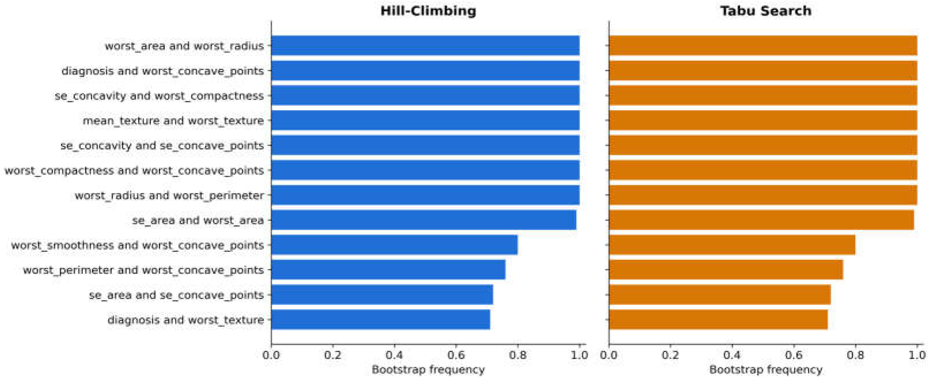
Figure 2.
Breast Cancer Wisconsin: BIC optimal versus BDeu optimal network, both Hill Climbing.
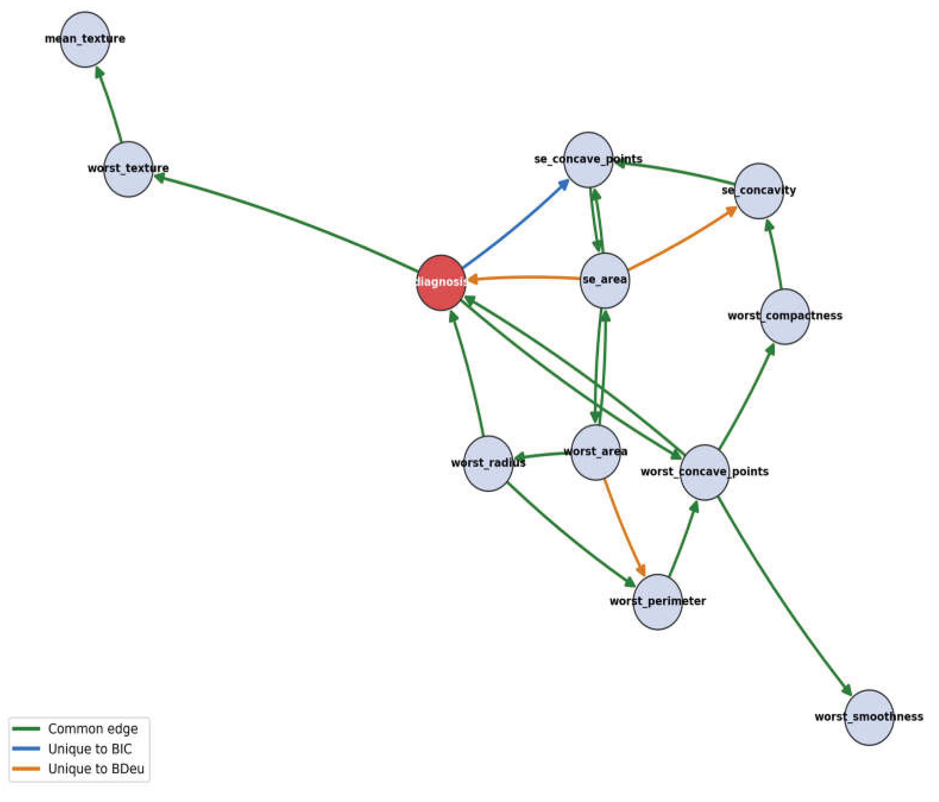
Figure 3.
Structural Hamming Distance across all three datasets: search algorithm agreement (left) and scoring function sensitivity relative to BIC (right).
Figure 3.
Structural Hamming Distance across all three datasets: search algorithm agreement (left) and scoring function sensitivity relative to BIC (right).
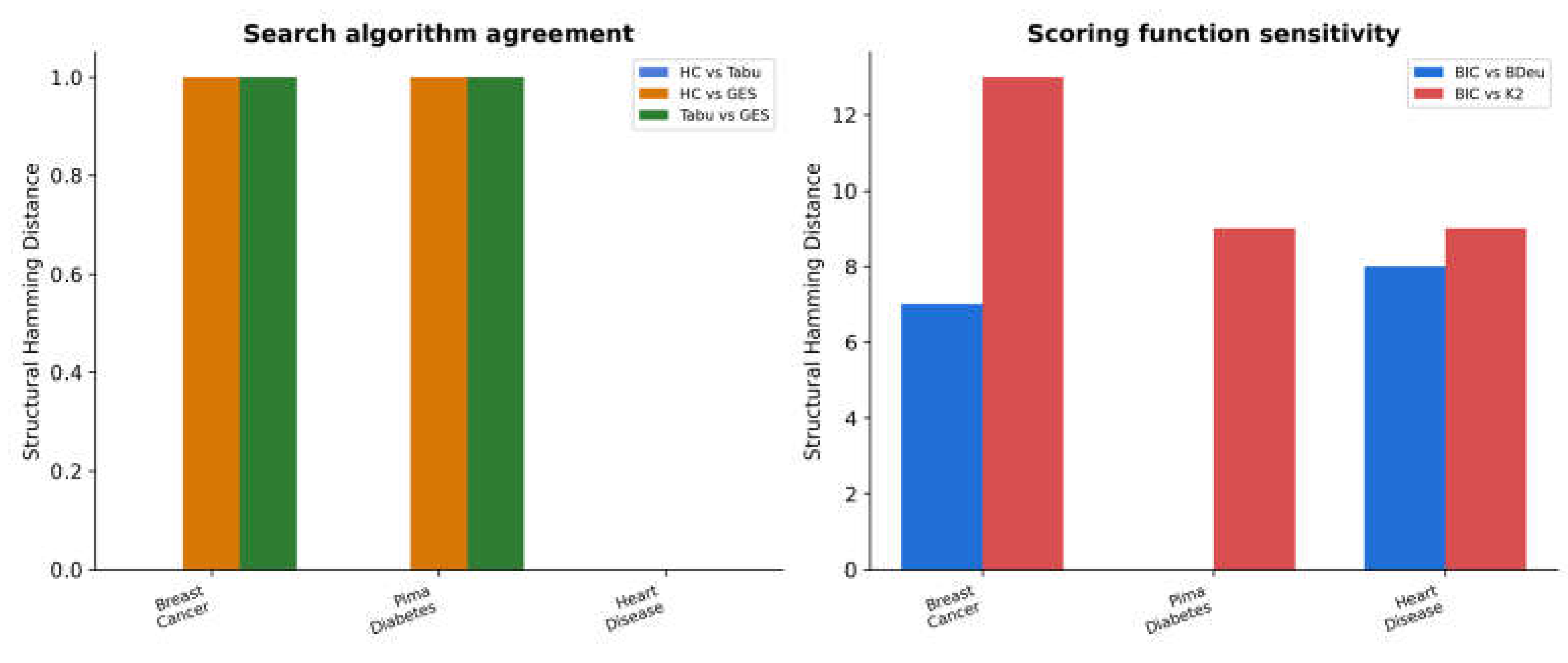

Table 1.
Dataset summary.
| Dataset | Patients | Predictors | Selected | Positive class | % positive |
| Breast Cancer Wisconsin | 569 | 30 | 11 | Malignant | 37.3 |
| Pima Indians Diabetes | 768 | 8 | 8 | Diabetes | 34.9 |
| UCI Heart Disease | 303 | 13 | 9 | Disease present | 54.5 |
Table 2.
Breast Cancer Wisconsin: selected features and mutual information rank (of 30).
| Step | Feature | MI rank | Mutual information |
| 1 | worst_radius | 1 | 0.414 |
| 2 | se_concavity | 17 | 0.122 |
| 3 | worst_smoothness | 20 | 0.082 |
| 4 | mean_texture | 19 | 0.106 |
| 5 | worst_area | 4 | 0.404 |
| 6 | se_area | 10 | 0.297 |
| 7 | worst_concave_points | 3 | 0.406 |
| 8 | worst_texture | 18 | 0.115 |
| 9 | se_concave_points | 16 | 0.131 |
| 10 | worst_perimeter | 2 | 0.411 |
| 11 | worst_compactness | 14 | 0.193 |
Table 3.
Search algorithm comparison under BIC.
| Dataset | Algorithm | Edges | BIC | Runtime (s) |
| Breast Cancer | Hill Climbing | 14 | -4745.98 | 0.78 |
| Breast Cancer | Tabu Search | 14 | -4745.98 | 0.76 |
| Breast Cancer | GES | 14 | -4745.98 | 12.27 |
| Pima Diabetes | Hill Climbing | 10 | -6353.21 | 0.44 |
| Pima Diabetes | Tabu Search | 10 | -6353.21 | 0.48 |
| Pima Diabetes | GES | 10 | -6353.21 | 5.32 |
| Heart Disease | Hill Climbing | 6 | -2585.69 | 0.39 |
| Heart Disease | Tabu Search | 6 | -2585.69 | 0.36 |
| Heart Disease | GES | 6 | -2585.69 | 3.92 |
Table 4.
Bootstrap SHD, all three algorithm pairs (100 resamples per dataset).
| Dataset | HC vs. Tabu | HC vs. GES | Tabu vs. GES | |||
| Mean | Median | Mean | Median | Mean | Median | |
| Breast Cancer Wisconsin | 0.00 | 0.0 | 7.25 | 7.0 | 7.25 | 7.0 |
| Pima Diabetes | 0.01 | 0.0 | 5.05 | 5.0 | 5.05 | 5.0 |
| Heart Disease | 0.00 | 0.0 | 3.07 | 3.0 | 3.07 | 3.0 |
Table 5.
Scoring function comparison under Hill Climbing (SHD relative to BIC).
| Dataset | Score | Edges | BIC yardstick | SHD vs. BIC |
| Breast Cancer | BIC | 14 | -4745.98 | 0 |
| Breast Cancer | BDeu | 16 | -4795.23 | 7 |
| Breast Cancer | K2 | 21 | -5680.86 | 13 |
| Pima Diabetes | BIC | 10 | -6353.21 | 0 |
| Pima Diabetes | BDeu | 10 | -6353.21 | 0 |
| Pima Diabetes | K2 | 14 | -6397.93 | 9 |
| Heart Disease | BIC | 6 | -2585.69 | 0 |
| Heart Disease | BDeu | 12 | -2602.41 | 8 |
| Heart Disease | K2 | 13 | -3024.09 | 9 |
Table 6.
Pooled summary: algorithm differences versus scoring function differences.
| Comparison | Median SHD | Mean SHD | |
| Algorithm differences (bootstrapped, pooled) | 900 | 3.0 | 3.42 |
| Scoring function differences (full sample) | 6 | 8.5 | 7.67 |
Table 7.
Sensitivity to the redundancy weight lambda (Breast Cancer Wisconsin, Hill Climbing, BIC).
| Distinct families | Edges | BIC | |
| 0.0 | 5 | 14 | -3283.01 |
| 0.5 | 6 | 14 | -4113.76 |
| 1.0 | 7 | 15 | -4637.15 |
| 1.3 | 8 | 14 | -4745.98 |
| 1.5 | 8 | 14 | -4745.98 |
| 2.0 | 8 | 14 | -4713.68 |
| 2.5 | 7 | 13 | -4807.52 |
| 3.0 | 7 | 13 | -4807.52 |
Table 8.
Sensitivity to the discretization level k (Breast Cancer Wisconsin, BIC).
| Edges | BIC | Features shared with | SHD(HC, Tabu) | |
| 3 | 14 | -4745.98 | 11/11 (reference) | 0 |
| 4 | 11 | -6057.70 | 10/11 | 0 |
| 5 | 11 | -7308.56 | 10/11 | 0 |
Disclaimer/Publisher’s Note: The statements, opinions and data contained in all publications are solely those of the individual author(s) and contributor(s) and not of MDPI and/or the editor(s). MDPI and/or the editor(s) disclaim responsibility for any injury to people or property resulting from any ideas, methods, instructions or products referred to in the content. |
© 2026 by the authors. Licensee MDPI, Basel, Switzerland. This article is an open access article distributed under the terms and conditions of the Creative Commons Attribution (CC BY) license (http://creativecommons.org/licenses/by/4.0/).
Copyright: This open access article is published under a Creative Commons CC BY 4.0 license, which permit the free download, distribution, and reuse, provided that the author and preprint are cited in any reuse.