

Submitted:
16 September 2026
Posted:
17 September 2026
You are already at the latest version
Abstract
Healthcare schools must place students in a limited number of internship wards. Manual planning is slow and may be difficult to inspect or explain, and internship assignment must satisfy department rotation, institution uniqueness, ward capacity, internship round, and student preference rules. This study compares a capacity-constrained regret heuristic with mixed-integer linear programming (MILP). The heuristic builds assignments from the options available at each decision. The MILP reduces the total weighted cost for the full cohort. Both methods were implemented in JavaScript within a standalone browser application. Method-specific records were also exported for a separate large language model explanation step. The evaluation used 133 students, three internship departments, and 101 healthcare institutions in Austria. Each method produced 399 valid placements. The MILP reduced the total weighted cost by 3.5% compared with the heuristic, while the heuristic was about 106 times faster in the recorded run. In one anonymized explanation case, both explanations passed four constraint checks and cited evidence from their source records. The heuristic explanation received higher scores for alternative coverage, uncertainty, and depth. The results show a trade-off between cohort cost, runtime, and the detail available for explaining an individual assignment.
Keywords:
internship scheduling
; mixed-integer linear programming
; regret heuristic
; transparency
; explainability
; large language model
MSC: 90B35; 90C11; 68T20
1. Introduction
1.1. Background
Austria faces pressure on healthcare staff and funding. This pressure is more noticeable in some rural areas [1]. Training places for nursing and other healthcare students can therefore be scarce. Nursing education also requires practical training. Students must complete all required internships before the final bachelor examination [2]. A nursing degree can require several internships in different clinical areas. Students may prefer or reject a city, institution, or department due to personal and social constraints. Ward limits must also be respected, and these rules make manual planning slow and difficult. Earlier scheduling tools reduced planning from days to minutes or cut monthly planning time by more than 79 percent [3,4].
Educational institutions apply different internship requirements. For example, internships can take place in separate rounds; a student cannot attend two places at the same time. Ward capacity is therefore linked to an internship round. The same ward can receive a new group in the next round. A planning tool must model these rules and reset the capacity between rounds. In some cases, schools may ask students to find places on their own. This choice can delay study completion when internship requirements are not met. A central scheduling tool can reduce this risk. Yet one fixed tool may not fit every school. Hence, each study program may need a tool that reflects its department rules, student order, and preference scale.
Still, automation does not solve every problem connected to internship assignments. Both staff and students need to see which rules were applied, and they must also understand why a particular internship place was selected. An unexplained result is hard to check or contest. NIST states that an explainable system should give evidence, be meaningful, reflect the real process, and state its limits [5]. Miller showed that useful explanations depend on the user and the question [6]. Rudin also argued for clear models in important decisions [7]. These points make transparency and explainability an important aspect of internship assignment planning.
1.2. Research Gap
Internship allocation tasks can be written as a graph problem. Mixed-integer linear programming (MILP) can find a low-cost solution. However, the results can still be hard to explain to a student. A simple heuristic can show each choice more directly. It can also apply list order and local rules, but it may produce a higher total cost for the cohort.
Recent work has studied nurse allocation, medical rotation schedules, and student placement [3,8,9,10]. Decision-support systems have also improved preference coverage, fairness, and planning time [4,11]. These studies focus on schedule quality and runtime. They do not report an evidence-linked LLM explanation test for each placement. Few studies compare exact allocation with heuristic approaches while also covering round-based capacity and method-specific explanation records.
1.3. Aim and Contribution
The goal of this paper is to compare two assignment methods: a capacity-constrained regret heuristic and a MILP model. Both methods will address institutional and student requirements in internship assignment tasks. Such requirements include assigning three internships to each student. Ensuring that every student receives an internship across designated departments: one Operativ, one Intern, and one Langzeit placement department. The department order across the three rounds is flexible. The three placements must use different institutions. The ward limit is applied in each round. The effective limit is two students when the source capacity is two or more. It is one student when the source capacity is one. Both methods, the heuristic and MILP, runs are separate, and the capacity use in one method does not affect the other method. Human-interpretable explanations are required for the assignment outputs produced by each method. A separate step is used to assess LLM-generated explanations of each method’s assignments. It uses the cohort assignment results and a method-specific record for the explanation of each internship assignment.
The paper also presents a proof of concept comprising the two methods, which are written in JavaScript. The PoC runs on one standalone HTML file in a browser. The tool reads institutional and students’ information through CSV files, calculates straight-line distance, creates assignments, and checks adherence to the internship assignment rules. The rest of this paper is structured as follows. Section 2 reviews related work. Section 3 defines the problem, presents both algorithms, and describes the proof of concept. Section 4 reports the scheduling and explainability results. Section 5 discusses the findings and related approaches. Section 6 concludes the paper.
2. Related Work
2.1. Healthcare Placement Scheduling
Nurse internship placement has several goals and these include short travel distances, fair assignments, capacity compliance, and training coverage. However, these goals may also raise conflicts. Shabani Afarani et al. used exact and hybrid methods for student nurse allocation [8]. Their work shows the value of comparing exact and fast methods. Medical rotation scheduling has similar limits. Castaño and Velasco compared exact and heuristic methods for trainee rotations [3]. Akbarzadeh and Maenhout used branch-and-price for medical student scheduling [9]. Shahraki et al. used MILP for monthly and daily trainee schedules [11]. Perelstein et al. used integer programming for resident shifts [4]. These studies show that exact models can improve schedule quality and planning time. They also show that each study program needs its own rules.
Genetic algorithms and simulated annealing provide additional approaches to solving scheduling problems. Metaheuristic methods provide approximate solutions when exact scheduling becomes difficult. Simulated annealing improves one schedule through small changes [22]. It can accept a higher-cost change during the early search, helping it escape a poor local solution. Knust and Xie combined simulated annealing with a mixed-integer programming model for nurse rostering [22]. The MILP exact model provided bounds for checking solution quality. The simulated annealing method provided good schedules within a practical search time. Their study also showed that neighbourhood design and parameter settings affect the final result.
Genetic algorithms search with a population of candidate schedules where new candidates are created through selection, crossover, and mutation. Aickelin and Dowsland used an indirect genetic algorithm for nurse scheduling [23]. Their decoder used problem-specific knowledge to construct schedules and reduce invalid results. Rivera et al. developed a capacity-aware genetic algorithm for resources with unequal limits [24]. Their work showed that the schedule representation and repair rules must reflect the resource constraints. Both genetic algorithms and simulated annealing use random decisions; therefore, their evaluations should include repeated runs and report the variation in cost, runtime, and constraint compliance.
2.2. Student Allocation Methods
Student allocation is often linked to preferences and limited project places. Abraham et al. studied algorithms for student-project allocation [14]. Thiruvady et al. compared integer programming with ant colony optimisation for industry placements [10]. These methods support the use of a common cost model for fair comparison.
Heuristic methods remain useful when scheduling rules change often. Akbarzadeh et al. used decomposition steps and candidate-control mechanisms to schedule medical students across hospital internships, and Udokwu et al. used explicit heuristic features to support traceable classification decisions [12,18]. The present algorithm adopts candidate control from the medical scheduling study. It uses the explicit-feature practice from the self-cited study only to structure the decision log.
2.3. Explanation of Optimisation Results
Explainability is important for addressing questions about bias and transparency in internship assignments. An LLM can turn structured decision data into plain text; however, it should not be treated as the solver. An LLM may struggle with rule-based assignments because its output is probabilistic and may contain unsupported statements [19]. It can still provide an explanation layer for an existing method. Phillips et al. defined explanation, meaningfulness, explanation accuracy, and knowledge limits as four key principles [5]. Miller found that people often prefer short and contrastive explanations [6]. Zhao et al. reviewed methods for explaining LLM outputs [15]. These works support a checked and narrow explanation task, providing additional interpretability to the users. To ensure the trustworthiness of these explanations, controls are required on generated explanations. Pan et al. combined an LLM with a deterministic symbolic solver to check logical reasoning [19]. Hence, users must understand the reasoning logic behind LLM outputs, and when they provide explanations, additional controls are needed to ensure that the interpretations provided by LLMs are trustworthy. Earlier works analyzed ethical and trust issues when LLMs are used in developing user-facing applications, and explored controls necessary for trustworthy LLM-integrated applications [13,17].
3. Materials and Methods
This section provides the materials and methods that form the solutions to addressing the internship assignment problems for nursing students. First, the internship assignment tasks are formalized as a graph problem, and the application of MILP and heuristic regret approaches is formally described. Later, the implementation of the PoC as well as the method adopted for assessing the explainability of the assignment outputs are described.
3.1. Problem Formalization
3.1.1. Network Graph
The allocation problem is represented as a layered graph. The first layer contains students and the next layers contain postal areas, health institutions, departments, and wards. Three round nodes represent the internship periods. A postal area is represented by its centroid. Postal-code centroid data can be obtained from an open geographic source [21].
An edge links a student’s location to an institution location. Its base value is the distance between the two postal centroids. Other edges hold student preferences. A ward node holds its source capacity. A placement edge also holds its assigned round. A past placement can be stored as a blocked edge. The current proof of concept uses default preference values if no preference data is provided.
Figure 1 shows the graph layers. Distance and preferences set the path cost. The effective ward capacity limits the number of paths in each round.
3.1.2. Sets and Parameters
Let S be the set of students. Let H be the set of institutions. Let denote the three required departments: Operativ, Intern, and Langzeit. Let be the internship rounds. Each student must complete three internship rounds. Let be the wards for institution h and department d. The source capacity of ward w is . Its effective capacity in one round is
An additional rule ensures that a ward cannot receive more than two students in one internship round. Hence, the effective capacity of one institution and department in one round is
Since the students cannot be in more than one internship place at the same time, this capacity is available again in every round. It is also reset before each assignment method starts.
Let be the centroid distance from student s to institution h. Let , , and be the preference factors for location, healthcare institution, and department, respectively. Their default value is one. The weighted path cost is
This cost is a relative score of travel distance (it is not a travel fare). A lower score represents a better selection for the student.
3.1.3. Exact Model
Placement Decision and Objective: The binary variable is one when student s is placed at institution h in department d. The placement objective is
Every student receives one placement in every department:
The three placements use distinct institutions:
The aggregate institution and department limit across the three rounds is
Round and Ward Decision: The binary variable is one when a selected placement uses ward w in round t. Each selected placement receives one ward and one round:
Each student receives one placement in each round:
Ward capacity is enforced separately in every round:
All and values are binary. Round assignment does not change the path cost, but only creates a feasible time and ward schedule.
3.2. MILP and Heuristics Regret Algorithms and Implementation
3.2.1. Adapted MILP Algorithm
The implemented MILP method has two stages to address the specific requirements of the nursing internship scheduling tasks. The first stage selects an institution and department for each required placement, and the second stage assigns the selected placements to wards and internship rounds.
Let
be the set of valid student, institution, and department paths. A path belongs to when the student and institution coordinates are valid and institution h offers department d.
For each , define
The weighted path cost is
where is the centroid distance. The parameters , , and are the location, institution, and department preference factors. Their default value is one.
The first-stage objective is
Every student must receive one placement in each department:
There are three required departments. Therefore, Equation (15) also gives
The three placements of a student must use different institutions:
Let
be the effective capacity of ward w in one internship round. The capacity of institution h and department d in one round is
There are internship rounds. The aggregate capacity available across the three rounds is therefore . The first-stage capacity constraint is
The first-stage decision variables satisfy
Let denote an optimal solution of Equations (14)–(21). The second stage assigns each selected path to one ward and one round.
Define
Every selected first-stage path must receive one ward and one round:
Every student must receive one placement in each round:
Ward capacity is applied separately in every round:
The second-stage decision variables satisfy
Feasibility of the Two-Stage Decomposition: The feasibility of the second stage follows from the structure of the current problem. Each student receives three placements in the first stage, with one placement in each department. The aggregate constraint in Equation (20) ensures that an institution-department pair receives no more than placements across the three rounds. The same capacity is available again in every round.
This relationship can be viewed as a bipartite graph, where one side contains the students and the other side contains the institution-department pairs. Each selected placement is an edge between both sides, and every student has three edges. The capacity of each institution-department pair can be divided into identical units. Each unit then receives at most three edges. These edges can be separated into three groups so that every student has one edge in each group and every capacity unit has at most one edge in each group. The three groups represent the internship rounds.
Each institution-department pair therefore receives at most students in one round. Since
these students can be distributed among its wards without exceeding the effective ward capacities. The second stage can therefore find values of that satisfy Equations (23)–(25).
This result also depends on the assumptions (requirements) used in the current implementation, where the Ward capacities are equal in all three rounds and reset after each round. This is necessary because the students cannot participate in more than one internship at the same time. Hence, students have no forbidden rounds or ward-specific restrictions. If such rules are added later, the first-stage aggregate constraint may no longer guarantee a feasible second stage. An integrated model or a recovery step would then be required.
Secondary Ward and Round Model: The second-stage implementation uses a small ordering coefficient. Let be the fixed index of ward w. Define
Equation (28) does not provide a unique round assignment. Equation (24) assigns exactly placements to each round. Therefore,
This value is constant for every feasible solution. The round term does not break round symmetry. The ward-index term can give preference to lower-indexed wards. However, several student-round assignments can still have the same objective value.
The solver may return any optimal second-stage solution. This does not affect the weighted path cost because is independent of the ward and round. It also does not affect feasibility. The returned schedule is recorded and checked against every assignment constraint. A unique round arrangement is not claimed, and a separate lexicographic procedure would be required if exact repeatability were needed.
The final weighted cost is
The objective depends only on x. The feasibility proposition shows that every first-stage solution satisfying the current assumptions can be decomposed into a valid ward-round schedule. The method therefore produces an optimal weighted institution-department assignment under the stated assumptions. It does not assign students in list order.
3.2.2. Capacity-Constrained Regret Heuristic
The heuristic assigns one task at a time. Where a task is a student-department pair. The initial task set is
Each student has three department tasks. Therefore,
Let q be the decision number. Let be the set of institutions already used by student s before decision q. Let be the set of rounds already used by the student. Initially,
Let be the remaining capacity of ward w in round t before decision q. Each round starts with an independent capacity balance:
The remaining capacity of institution h and department d in round t is
For an unassigned task , define the feasible option set as
An option is feasible when its institution and round are unused by the student and a ward place remains. The number of feasible path-round options is
Let be the fixed alphabetical index of institution h. The options in are ordered by
The weighted cost is the main ordering value. The round number is the first tie-break. The institution index is the next tie-break.
Let
be the first option in this order. Let be the next option when it exists. Their costs are
The path-round regret value is
Let be the position of student s in the input file. Let be the fixed department order. Define lexargmin as the argument with the smallest tuple in lexicographic order. The next task is
Equation (41) first selects the task with the fewest feasible options. It then selects the task with the largest regret. Student list position is the final comparison between different students. The department index resolves a remaining tie between tasks belonging to the same student.
The selected institution and round are given by
Let be the fixed alphabetical index of ward w. The selected ward is
The heuristic first uses the ward with the largest remaining capacity. The ward index resolves an equal-capacity tie.
Only the selected ward balance in the selected round is reduced:
The student’s used institution and round sets are updated as
The corresponding sets of all other students remain unchanged. The selected task is removed:
The process continues for
If for any remaining task, the current heuristic state is infeasible. The implementation stops and reports the missing placement. Otherwise, the final heuristic cost is
Interpretation of Path-Round Regret: The alternative represented in this heuristic is a path-round pair. It is not an institution alone. The pairs and are different decisions because every round has a separate capacity balance. Selecting consumes round t for the student. It also reduces capacity only in that round.
The regret value in Equation (40) measures the cost of losing one feasible path-round option. It does not measure the cost of losing an institution across all rounds. Suppose that the first two options use the same institution in different rounds. Their costs are equal because the objective has no round cost. The regret is then zero. This result is intentional. It means that the loss of one round option causes no immediate cost increase because an equal-cost option remains in another round.
Zero regret can occur often during early decisions since several rounds may still be available for the same institution at that time. Positive regret becomes more important as student rounds and ward capacities are consumed. The term path-round regret distinguishes this measure from institution-level regret. An institution-level measure would remove duplicate institutions before comparing costs. It would define a different heuristic and require a new evaluation.
The heuristic selects the lowest-cost option only for the task chosen at decision q. It does not minimize Equation (49) over all complete schedules. This distinguishes the heuristic from the cohort-wide MILP method.
3.2.3. Proof-of-Concept Implementation
Data Input: The proof of concept is one standalone HTML file. It accepts a student CSV file and an institution-and-ward CSV file. A student row contains a name, ID, postal code, latitude, and longitude. An institution row contains the institution, postal code, latitude, longitude, department, ward, and source capacity. An optional CSV file contains the preference factors. The source files were used to create the built-in test data. The tool derives the political district, or Politischer Bezirk, from the GeoNames postal-code file [21]. A postal code can cover more than one district. In that case, the tool retains all reported district names. Invalid postal codes are reported before a run. The tool does not send input data to a server.
Distance and Solvers: The tool calculates great-circle distance with the Haversine formula [20]. Both assignment methods are written in JavaScript. The MILP uses a JavaScript linear programming library. The library is embedded in the standalone HTML file. The first-stage and second-stage models run in browser workers. The heuristic and MILP are separate operations. Each method starts from the original effective ward capacities. No assignment or capacity balance is transferred from one method to the other.
Both MILP stages were solved with javascript-lp-solver, version 1.0.3 [25]. This package is a pure JavaScript linear and mixed-integer programming solver. It uses the simplex method for linear programming relaxations and a branch-and-cut procedure for integer variables. The internal JavaScript backend was used. No external native solver, WebAssembly module, or server service was called. The embedded solver ran inside browser Web Workers. The models were passed to the library through its JSON interface. All assignment variables were declared as integer variables. The application did not set the model’s relative MIP tolerance. The library default of zero was therefore used. A nonzero MIP gap was not permitted as an early stopping condition. No solver time limit was specified. The calls therefore used no application-defined time limit. No explicit numerical precision argument was passed to the solver. The embedded build used its default numerical precision of .
Output and Validation: The tool presents both methods in one searchable result view. Each assignment row states the student, round, department, institution, ward, distance, and weighted cost. The CSV export also contains the student name, political district, and internship round. The heuristic JSON export records the feasible options available at each decision. It also records the option count, path-round regret, student list position, selected ward, and capacity change. The MILP JSON export records the selected path, solver status, cohort cost, path rank, and ward use. The tool reports total cost, runtime, and completed assignments. A final validation checks the number of placements, one placement per round, department coverage, institution uniqueness, distance coverage, and ward capacity in every round.
3.3. Evaluation Design
The evaluation used student data, healthcare institution data, and optional preference data. It also used measures based on the weighted assignment costs.
Dataset: The test used 133 student records; all student IDs and postal codes were loaded, and their political districts were resolved from GeoNames. The institution file contained 101 institutions and 380 ward rows. The source capacities provided 1381 places. The effective capacity was 726 places in each round after applying the limit of two students per ward. Default preference factors were used. Each student required three internships. Each student required one placement in Operativ, Intern, and Langzeit. This gave 399 placements per method. Each round required 133 simultaneous placements.
Measures: The main measure was total weighted path cost. Lower cost was better. The checks also covered rule compliance and completion. Runtime was recorded during one proof-of-concept run. The test used the Microsoft Edge browser on a standard work laptop. Capacity was checked by method, round, institution, department, and ward. This grouping tests both reset rules. A ward can be reused in another round. The two methods have independent capacity balances. Therefore, an assignment from one method cannot consume capacity in the other method.
4. Results
This section describes the results obtained after performance and explainability experiments that compared outputs from both the MILP and Heuristic regret approaches.
4.1. Scheduling Performance
Table 1 gives the scheduling results for the evaluated 133 students. Both methods completed all 399 placements where every student received one placement in each round. Every student also received all three departments at three different institutions. Both methods passed the per-round ward-capacity checks.
The heuristic total weighted cost was 5,467.5. The MILP total weighted cost was 5,275.2. These costs represent the total kilometer distance that will be traveled by the students across the three internship rounds. The MILP reduced the total cost by 3.5 percent while the recorded heuristic time was 1,185 ms. The recorded MILP time was 125,635 ms. The MILP time includes placement optimisation and exact round scheduling.
Table 2 presents the distribution of student-level weighted costs. We summed the three internship costs for each student. The MILP reduced the mean cost from 41.1 to 39.7. It also reduced the median cost from 37.7 to 36.8. This shows that the MILP produced lower costs for the cohort and for the typical student. However, the maximum student cost remained 194.6 under both methods. Therefore, reducing the total cohort cost did not reduce the highest individual cost.
The result shows the expected trade-off. The MILP considers all placement costs in one cohort model. It then finds a valid round and ward schedule. The heuristic makes each choice from the current options. This makes its path easier to review. It also finishes much faster in this test.
4.2. Explainability Evaluation
4.2.1. Experimental Method
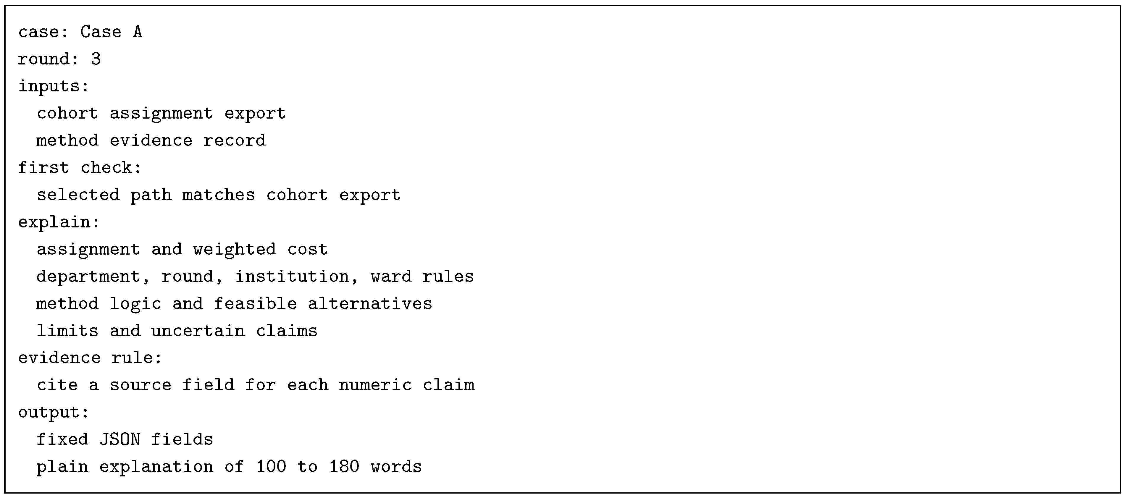
The explainability experiment used one student with an edge-case assignment in the third internship round. For the purpose of the experiment, the student was renamed Case A. Also, Institution names were changed to H1, H2, and H3. Ward labels were shortened. Names, postal codes, and student identifiers were removed from the paper. The same case was tested once for the regret heuristic and MILP. The LLM received the cohort assignment export and one method record. The heuristic record was a decision log for the selected assignment. The MILP record described the final solution for the selected case. The LLM was used to explain both assignments but did not change the actual assignments.
| Listing 1. Summarized explanation prompt structure |
 |
| Listing 2. Summarized method evidence structure |
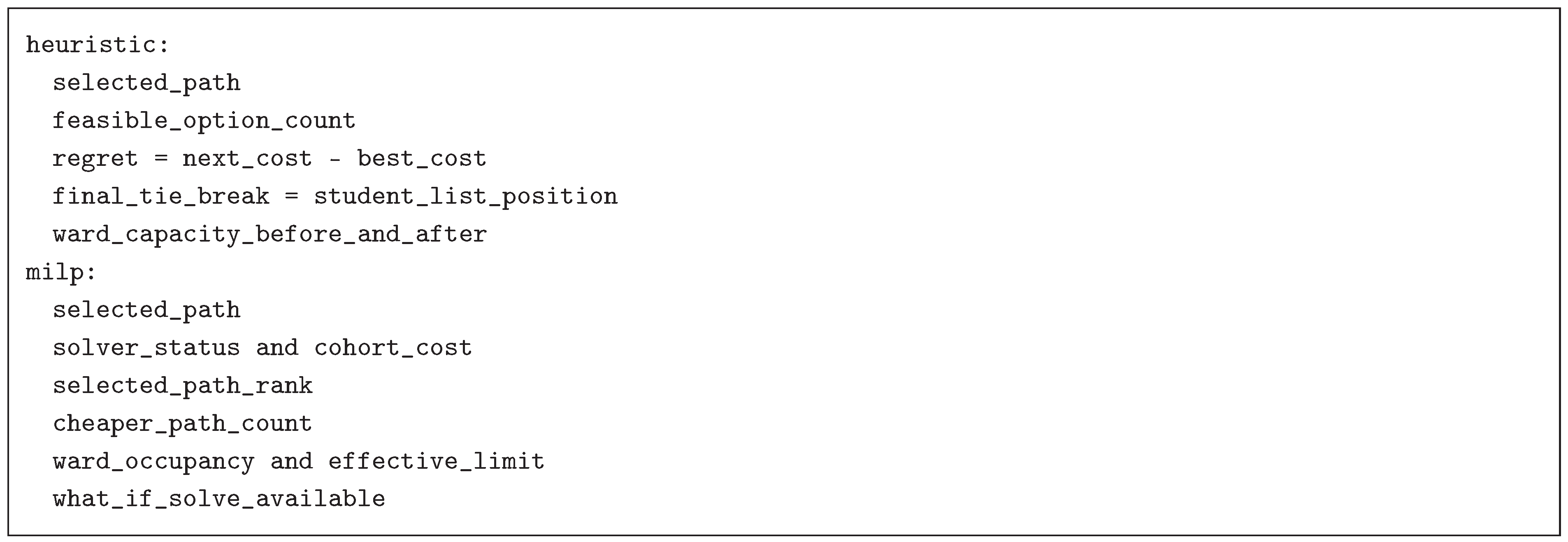 |
The records were exported when the tool finished both methods. The evaluator selected one result row for Case A and Round 3. The “Heuristic log JSON” control function was used to find the matching event in the stored decision log. That event was captured when the heuristic made the assignment. It held the ranked options, regret value, list position, tie-break facts, and capacity change. The “MILP record JSON” control used the same student and round. An explanation record was built from the completed MILP solution. The record held the solver status, cohort cost, selected-path rank, ward use, and the first ten ranked paths. For the selected student case, the Heuristics regret decision log, the MILP explanation record, and the overall assignment data for all the students were all exported for the explainability experiment.
An open-weight LLM (DeepSeek-R1) was used for the explanation experiment, and all student and organizational data were anonymized before they were fed into the model. The prompt first asked the model to match the selected path with the cohort export. It then asked for the assignment reason, cost, constraints, method logic, alternatives, and limits. Every numeric claim required a source field. The response used fixed JSON fields and a plain explanation of a maximum of 180 words. Listing 1 shows the prompt structure.
The two records for data used in the explainability experiment exposed different method logic. The heuristic log stored the options available at the decision time. It also stored regret, list position, and capacity before and after assignment. The MILP record stored solver status, cohort cost, path rank, and ward use. It did not contain a what-if solve. Listing 2 gives the anonymized record structure.
4.2.2. Evaluation Properties
The evaluation used factual correctness, evidence, quality, depth, alternative coverage, and stated uncertainty. These properties align with the four principles from Phillips et al. [5]. Correctness supports explanation accuracy. Quality and depth support meaningfulness. Uncertainty supports knowledge limits. Zhao et al. also showed the need to test whether an LLM explanation reflects its evidence [15].
One human evaluator checked the generated explanations. The evaluator marked the department, round, institution, and ward claims as correct or incorrect. Evidence references were marked yes or no. Numeric ratings were entered for alternatives, uncertainty, correctness, quality, and depth. The recorded scale used 3 for a good score, 1 for a poor score, and 2 for an in-between score.
4.2.3. LLM Explanation Results
The regret heuristic produced a decision log in JSON. The MILP produced a separate explanation record in JSON for the same student. Table 3 summarizes the evidence reported in both explanations. This includes the selected path, weighted cost, method evidence, alternative evidence, capacity evidence, and stated limits. Table 4 gives the human assessment of the two explanations. The first column contains the assessment properties. The other columns contain the ratings for each method.
The categorical checks show that both explanations stayed consistent with the records and both received the same scores for correctness and quality. The heuristic response received higher scores for alternatives, uncertainty, and depth. Its log contained the exact decision-time option set and the next-best cost. The MILP record showed a cohort optimum, but it had no what-if solve. This difference may explain the lower depth score for the MILP response.
5. Discussion
5.1. Comparison of the Two Methods
The performance comparative analysis shows that both methods completed 399 placements and passed every scheduling check. However, the MILP had the better cost result. Its total weighted cost was 5,275.2. This was 3.5 percent below the heuristic cost of 5,467.5. The heuristic had the better runtime. It finished in 1,185 ms. The MILP needed 125,635 ms. The heuristic was therefore about 106 times faster in this run. Still, both methods have the same student maximum assignment at 194.6 across the three internship rounds.
The methods also differed in transparency. The heuristic recorded the options that existed when each choice was made. It showed the best cost, next-best cost, regret, capacity change, and final list-order tie-break. The MILP record showed that the full cohort result was optimal. It also showed the selected path rank and cohort cost. It could not show the exact effect of forcing a different individual path because no what-if solve was run.
Both LLM explanations passed the four constraint checks. Both cited evidence and received a recorded value of 3 for correctness and quality. The heuristic explanation had higher recorded values for alternative coverage, uncertainty, and depth. Its decision log gave direct facts about the next option. The MILP explanation had less local detail because the assignment came from one joint cohort solve. These findings support the expected trade-off. MILP gave a lower cohort cost. The heuristic gave faster and more direct local reasoning. The explanation result is limited to one case and one evaluator.
The two methods support different planning priorities. MILP considers the cost of the full cohort. The regret heuristic also applies student list position as its final tie-breaker. This rule can represent a declared policy that rewards earlier preference submissions. It applies only when option count and regret are equal. Hence, if the main goal is to reduce cohort travel cost, MILP is the better choice in this test. If staff must also apply an accepted list-order rule and inspect each decision-time option set, the regret heuristic offers useful evidence.
5.2. Comparison with Other Scheduling Approaches
Earlier studies solved related problems with different goals. Castaño and Velasco used exact and metaheuristic methods for trainee rotations. Their spreadsheet tool reduced planning from several days to minutes [3]. Shabani Afarani et al. used an exact multi-objective method for small cases and a guided NSGA-II method for larger cases. Their best real-case result reduced total completion time across wards by 30.9 percent when compared with a manual schedule [8].
Other studies focused on preferences, fairness, and shifts. Shahraki et al. used MILP for monthly and daily trainee schedules. Their system covered 11 percent more rotation preferences, improved fairness by 19 percent, and met duty-hour rules for all trainees [11]. Perelstein et al. used integer programming for resident shifts. Their tool cut monthly planning time by 79 to 82 percent. It also reduced difficult shift patterns by 85.7 percent [4]. Thiruvady et al. used integer programming and ant colony optimisation for industry placements. Their integer model improved average allocations over manual results in most tested semesters [10].
These performance improvements presented as percentages in the earlier works cannot be compared directly with the results in this paper. The present evaluation did not compare automated and manual assignments. Both methods nevertheless completed the tested assignment within minutes. Earlier work reports that manual planning can take days to complete; hence the results in our current paper show high performance gain [3]. The present study instead compares two automated methods on the same data, costs, and rules. It identifies the planning priority supported by each method.
Metaheuristics have also been used in practical healthcare scheduling. Knust and Xie integrated simulated annealing into duty rostering software used with German and Austrian hospital data [22]. Aickelin and Dowsland developed a genetic algorithm for nurse rostering at a large UK hospital [23]. Rivera et al. also applied a genetic algorithm to operating-room scheduling with different room capacities [24]. These methods can be adapted to the internship problem. Simulated annealing could start with the valid schedule produced by the regret heuristic. It could then move one placement or swap placements between two students. A genetic algorithm could represent each complete schedule as a chromosome. Its crossover and mutation steps could produce new assignment plans. A repair step would preserve the three internship rounds, department rotation, institution uniqueness, and ward capacity rules. Both methods could use the same weighted cost as the MILP. Their cost, runtime, and constraint compliance could then be compared with the heuristic and MILP results. However, repeated runs would be required because both methods contain random decisions.
Our work extends the previous works on automated internship planning and scheduling with the LLM-integrated explanation layer. The reviewed scheduling papers report schedule quality, runtime, preferences, or fairness. However, they do not report a method-specific decision record and a checked LLM explanation for each selected placement. The heuristic export preserves the local choice event. The MILP export preserves solver and path evidence. The fixed prompt keeps the LLM separate from the assignment step. Human checks then compare the explanation with the source record. This supports review by staff and students, thereby making unsupported claims easier to identify.
6. Conclusions
Internship assignment has three linked problems. The first is the time needed for manual planning. The second is the need to apply rotation, preference, institution, and ward rules. The third is the need to make each result clear to staff and students. Automation can improve planning speed, but an unexplained result can still be hard to trust or contest. This paper compared two automated internship assignment methods. The regret heuristic made feasible choices from the currently available options. It used option count, regret, and student list order. The MILP lowered total cost for the full cohort. Both methods assigned three internships in three rounds, and a separate explanation step used method-specific JSON records. The LLM turned those records into plain text explanations.
The scheduling evaluation used 133 students, and the methods produced 399 valid placements. The MILP reduced total weighted cost by 3.5 percent, while the heuristic regret approach ran about 106 times faster. In the one-case explanation test, both outputs passed all four constraint checks and cited their evidence. The MILP method produced slightly better mean and median costs per student; however, the maximum cost per student across the internship rounds remained the same. Still, the heuristic explanation received higher scores for alternatives, uncertainty, and depth. Both explanations stated their evidence and limits correctly.
The study has some limitations. It used postal-code centroid distance and default preferences. For the explainability experiments, it tested one cohort and recorded runtime once. The explanation test evaluated one student and one evaluator. Future work will use actual route travel time and student preferences. Further evaluation will cover more cohorts, students, rounds, evaluation cases, and reviewers. These steps will support stronger claims about cost, transparency, and explanation quality.
Author Contributions
Conceptualization, CU, GS; methodology, CU, GS, HB, DD; software, CU, GS; validation, GS, RT; formal analysis, CU, RT; resources, DD; data curation, GS; writing, original draft preparation, CU; writing, review and editing, CU, GS, HB, DD, RT; project administration, CU, GS. All authors have read and agreed to the published version of the manuscript.
Funding
The authors declare no funding for this research.
Data Availability Statement
The student-level administrative data used in this study cannot be made publicly available because they contain potentially identifiable educational and location information. An anonymized dataset, along with the implementation and evaluation scripts, is available from the corresponding author upon reasonable request, subject to institutional data-protection requirements.
Conflicts of Interest
The author declares no conflicts of interest.
Abbreviations
The following abbreviations are used in this manuscript:
| CSV | Comma-separated values |
| GA | Genetic algorithm |
| LLM | Large language model |
| MILP | Mixed-integer linear programming |
| PoC | Proof of concept |
| SA | Simulated annealing |
References
- OECD. European Observatory on Health Systems and Policies. Austria: Country Health Profile 2025; OECD Publishing: Paris, France, 2025. [Google Scholar]
- Federal Ministry of Labour; Social Affairs; Health; Care and Consumer Protection. BGBl. II Nr. 152/2026; FH-Gesundheits- und Krankenpflege-Ausbildungsverordnung 2026 (FH-GuK-AV 2026). 25 June 2026. Available online: https://ris.bka.gv.at/Dokumente/Bundesnormen/NOR40278640/NOR40278640.html (accessed on 11 September 2026).
- Castaño, F.; Velasco, N. Exact and heuristic approaches for the automated design of medical trainees rotation schedules. Omega 2020, 97, 102107. [Google Scholar] [CrossRef]
- Perelstein, E.; Rose, A.; Hong, Y.-C.; Cohn, A.; Long, M.T. Automation improves schedule quality and increases scheduling efficiency for residents. J. Grad. Med. Educ. 2016, 8, 45–49. [Google Scholar] [CrossRef] [PubMed]
- Phillips, P.J.; Hahn, C.A.; Fontana, P.C.; Yates, A.N.; Greene, K.; Broniatowski, D.A.; Przybocki, M.A. Four Principles of Explainable Artificial Intelligence; NISTIR 8312; National Institute of Standards and Technology: Gaithersburg, MD, USA, 2021. [Google Scholar] [CrossRef]
- Miller, T. Explanation in artificial intelligence: Insights from the social sciences. Artif. Intell. 2019, 267, 1–38. [Google Scholar] [CrossRef]
- Rudin, C. Stop explaining black box machine learning models for high stakes decisions and use interpretable models instead. Nat. Mach. Intell. 2019, 1, 206–215. [Google Scholar] [CrossRef] [PubMed]
- Shabani Afarani, H.; Atighehchian, A.; Nazari, R. Multi-objective student nurse allocation problem during training using exact and hybrid heuristic-metaheuristic methods. Sci. Rep. 2026, 16. [Google Scholar] [CrossRef]
- Akbarzadeh, B.; Maenhout, B. An exact branch-and-price approach for the medical student scheduling problem. Comput. Oper. Res. 2021, 129, 105209. [Google Scholar] [CrossRef]
- Thiruvady, D.R.; Morgan, K.; Bedingfield, S.E.; Nazari, A. Allocating students to industry placements using integer programming and ant colony optimisation. Algorithms 2021, 14, 219. [Google Scholar] [CrossRef]
- Shahraki, N.; Sir, M.Y.; Prindle, T.; Ramar, K. A decision-support system to schedule rotations for trainees Formalizing and simulating the token aspects of blockchain-based research collaboration platform using game theory. In ATS Sch.;Mathematics; Udokwu, C., Ed.; 2022; Volume 3 12, pp. 425–432 3252. [Google Scholar] [CrossRef]
- Udokwu, C.; Mirhosseini, S.A.M.; Craß, S. Heuristics analyses of smart contracts bytecodes and their classifications. Electronics 2026, 15, 41. [Google Scholar] [CrossRef]
- Udokwu, C.; Dwivedi, V.; Buick, A.; Keers, J.; Liu, J. An agentic AI marketplace for prelitigation analyses with ZKP-integrated ethical verifications. Front. Blockchain 2026, 9. [Google Scholar] [CrossRef]
- Abraham, D.J.; Irving, R.W.; Manlove, D.F. Two algorithms for the student-project allocation problem. J. Discret. Algorithms 2007, 5, 73–90. [Google Scholar] [CrossRef]
- Zhao, H.; Chen, H.; Yang, F.; Liu, N.; Deng, H.; Cai, H.; Wang, S.; Yin, D.; Du, M. Explainability for large language models: A survey. ACM Trans. Intell. Syst. Technol. 2024, 15, 20. [Google Scholar] [CrossRef]
- Udokwu, C.; Voicu-Dorobantu, R.; Ogunyemi, A.A.; Norta, A.; Sturua, N.; Craß, S. Leveraging blockchain for ethical AI: Mitigating digital threats and strengthening societal resilience. Future Internet 2025, 17, 309. [Google Scholar] [CrossRef]
- Udokwu, C.; Dwivedi, V.; Buckchash, H. Trustable LLM applications with privacy-preserving computations and decentralized tech stacks. SSRN 2026. [Google Scholar] [CrossRef]
- Akbarzadeh, B.; Wouters, J.; Sys, C.; Maenhout, B. The scheduling of medical students at Ghent University. Inf. J. Appl. Anal. 2022, 52, 303–323. [Google Scholar] [CrossRef]
- Pan, L.; Albalak, A.; Wang, X.; Wang, W. Logic-LM: Empowering large language models with symbolic solvers for faithful logical reasoning. In Findings of the Association for Computational Linguistics: EMNLP 2023; Association for Computational Linguistics: Singapore, 2023; pp. 3806–3824. [Google Scholar] [CrossRef]
- Bullock, R. Great circle distances and bearings between two locations. MDT. 2007, pp. 1–3. Available online: https://dtcenter.org/sites/default/files/community-code/met/docs/write-ups/gc_simple.pdf (accessed on 11 September 2026).
- GeoNames. Postal Code Files. Available online: https://download.geonames.org/export/zip/ (accessed on 11 September 2026).
- Knust, F.; Xie, L. Simulated annealing approach to nurse rostering benchmark and real-world instances. Ann. Oper. Res. 2019, 272, 187–216. [Google Scholar] [CrossRef]
- Aickelin, U.; Dowsland, K.A. An indirect genetic algorithm for a nurse-scheduling problem. Comput. Oper. Res. 2004, 31, 761–778. [Google Scholar] [CrossRef]
- Rivera, G.; Cisneros, L.; Sánchez-Solís, P.; Rangel-Valdez, N.; Rodas-Osollo, J. Genetic algorithm for scheduling optimization considering heterogeneous containers: A real-world case study. Axioms 2020, 9, 27. [Google Scholar] [CrossRef]
- Wolcott, J.W. javascript-lp-solver, version 1.0.3. 2026. Available online: https://www.npmjs.com/package/javascript-lp-solver/v/1.0.3 (accessed on 13 September 2026).
- Yao, Y.; Duan, J.; Xu, K.; Cai, Y.; Sun, Z.; Zhang, Y. A survey on large language model security and privacy: The good, the bad, and the ugly. High-Confid. Comput. 2024, 4, 100211. [Google Scholar] [CrossRef]
Figure 1.
Layered graph for the internship allocation problem.


Table 1.
Scheduling performance results.
| Measure | Heuristic | MILP |
|---|---|---|
| Students completed | 133 | 133 |
| Placements made | 399 | 399 |
| Round 1 placements | 133 | 133 |
| Round 2 placements | 133 | 133 |
| Round 3 placements | 133 | 133 |
| Operativ placements | 133 | 133 |
| Intern placements | 133 | 133 |
| Langzeit placements | 133 | 133 |
| Total weighted cost | 5,467.5 | 5,275.2 |
| Cost reduction | 0.0% | 3.5% |
| Rule checks passed | Yes | Yes |
| Runtime | 1,185 ms | 125,635 ms |
Table 2.
Distribution of combined student-level weighted costs across three internship rounds.
| Student-Level Cost Measure | Heuristic | MILP |
|---|---|---|
| Mean cost | 41.1 | 39.7 |
| Median cost | 37.7 | 36.8 |
| Maximum cost | 194.6 | 194.6 |
Table 3.
Anonymized evidence reported in the LLM explanations.
| Item | Heuristic explanation | MILP explanation |
|---|---|---|
| Selected path | Intern, Institution H1, Ward I3 | Operativ, Institution H2, Ward O4 |
| Weighted cost | 35.76; distance and all factors were checked | 24.61; distance and all factors were checked |
| Method evidence | 34 feasible options; regret 6.45; selected path was best at decision time | Solver status Optimal; cohort cost 5,275.20; selected path rank was 2 |
| Alternative evidence | Next path cost was 42.21 at Institution H3 | One cheaper individual path existed; 10 alternatives were recorded |
| Capacity evidence | Remaining ward capacity changed from 2 to 1 | Ward occupancy was 2 of an effective limit of 2 |
| Stated limit | The heuristic did not claim a cohort optimum | No what-if solve was available; the exact cause of the trade-off was not claimed |
Table 4.
Recorded human evaluation for Case A.
| Property | Heuristic | MILP |
|---|---|---|
| Department constraint | Correct | Correct |
| Round constraint | Correct | Correct |
| Institution constraint | Correct | Correct |
| Ward constraint | Correct | Correct |
| Evidence references | Yes | Yes |
| Alternative explanation | 3 | 2 |
| Uncertainty explanation | 2 | 1 |
| Plain-text correctness | 3 | 3 |
| Plain-text quality | 3 | 3 |
| Plain-text depth | 3 | 1 |
Disclaimer/Publisher’s Note: The statements, opinions and data contained in all publications are solely those of the individual author(s) and contributor(s) and not of MDPI and/or the editor(s). MDPI and/or the editor(s) disclaim responsibility for any injury to people or property resulting from any ideas, methods, instructions or products referred to in the content. |
© 2026 by the authors. Licensee MDPI, Basel, Switzerland. This article is an open access article distributed under the terms and conditions of the Creative Commons Attribution (CC BY) license (http://creativecommons.org/licenses/by/4.0/).
Copyright: This open access article is published under a Creative Commons CC BY 4.0 license, which permit the free download, distribution, and reuse, provided that the author and preprint are cited in any reuse.