
Submitted:
14 September 2026
Posted:
16 September 2026
You are already at the latest version
Abstract
Copper is recognized as a strategic mineral resource supporting the energy transition and digital development. Based on copper trade data from 2015 to 2024 for 146 countries, the copper industry chain is divided into four functional layers: the raw material layer, the refining and processing layer, the recycling layer, and the equipment layer, for which directed weighted trade networks are constructed. In particular, the equipment layer is used as a proxy for investment in copper-processing capacity and manufacturing capability. Complex network methods, community detection, and dynamic targeted-node attack simulations are employed to examine the structural evolution and resilience of the global copper industry chain trade network. The following results are obtained: (1) Significant hierarchical heterogeneity is exhibited in the global copper industry chain trade network. The refining and processing layer is the densest, while the equipment layer increasingly converges toward it, and both show a trend toward concentration in core countries in the later period. (2) China’s core position is systematically strengthened across all layers. Raw material exports are dominated by Chile and Peru; in 2024, Chile is replaced by the Democratic Republic of the Congo as the largest trade corridor to China in the refining and processing layer; in the recycling layer, a shift from dominance by traditional developed economies toward a multi-node collaborative East Asia–Southeast Asia pattern is observed; the equipment layer is shifted from a pattern led by the United States and Germany to one in which China is made the dominant hub of both supply and demand. (3) Marked reorganization is observed in the community structure. In the raw material layer, Chile is transferred to the China-centered community. In the refining and processing layer, the China-centered community is expanded toward the Asia-Pacific and Africa. In the recycling layer, the trans-Pacific community is gradually integrated. In the equipment layer, three coexisting blocs are formed: an Asia-Pacific community, a Europe–Africa transcontinental community, and Americas communities characterized by North–South differentiation. (4) Network resilience is ranked in the following order: the refining and processing layer > the equipment layer > the recycling layer > the raw material layer. In 2024, resilience is markedly weakened in the refining and processing and recycling layers; some recovery is observed in the raw material layer; the equipment layer remains relatively stable overall.
Keywords:
complex network
; global copper industry chain
; trade network
; trade pattern
; network resilience
1. Introduction
Against the backdrop of accelerating global energy transition and digitalization, the strategic importance of copper as a critical basic raw material has become increasingly prominent. The International Energy Agency (IEA) and the U.S. Geological Survey (USGS) have indicated that clean energy technologies, data centers, and artificial intelligence infrastructure will substantially increase copper demand. Meanwhile, global copper mine supply is highly concentrated in a small number of countries, including Chile, Peru, and the Democratic Republic of the Congo. Consequently, rising resource nationalism and geopolitical conflicts have significantly intensified uncertainty in the copper supply chain [1,2]. From the perspective of resource distribution, exploration, and development, Chen Xiufa et al. [3] pointed out that global copper reserves are concentrated in South America, with South America serving as the major export center and Asia as the major import and consumption center. Zhu Qing et al. [4] further noted that declining copper ore grades, the concentration of smelting capacity in Asia, and unstable supplies of recycled copper raw materials are jointly reshaping the global copper industry chain through structural changes across different stages. Against this background, a layered characterization of the global copper trade network and an assessment of its resilience from the perspective of the industry chain can help systematically clarify the differences, evolutionary characteristics, and potential risks of trade structures across different stages.
The division of the copper industry chain should be understood not merely as a matter of product classification, but within the framework of the global value chain (GVC) division of labor. Gereffi et al. [5] argued that the governance modes of global value chains are determined by transaction complexity, codifiability, and supplier capabilities, and that substantial differences exist among different stages in terms of power structure and value-adding capacity. Based on this theoretical perspective, the copper industry chain is divided in this study into four functional layers: the raw material layer, the refining and processing layer, the recycling layer, and the equipment layer. The first two constitute the upstream and midstream segments of copper material flows; the recycling layer reflects the functions of the circular economy and the reallocation of secondary resources; and the equipment layer, which covers trade in specialized machinery for smelting, rolling, continuous casting, and related processes, reflects the investment layout of a country’s copper processing and manufacturing capacity as well as its demand for technological upgrading. Compared with classification by product category, division by functional layer can more effectively reveal the position of each stage in the value chain division of labor and the interdependence among different stages. Moreover, it provides a theoretical basis for identifying structural vulnerabilities across different layers.
Complex network methods have been widely applied in studies of resource trade. In the field of copper trade, previous studies have examined individual products such as copper ores [6], refined copper [7,8], and copper scrap [9], revealing the “core-periphery” structure of trade networks, multi-core communities, and differentiated roles of major countries [10]. However, studies focusing on individual products are unable to fully reveal the structural differentiation within the copper industry chain. Some scholars have attempted to construct multi-product copper trade networks from an industry-chain perspective [11,12] and have further introduced network resilience assessment frameworks [13,14,15]. These studies have found that upstream segments are more vulnerable to external shocks than downstream segments and that China is gradually evolving into a hub covering the entire industry chain [14,15]. Studies by Albert et al. [16] and Crucitti et al. [17] demonstrated that scale-free networks exhibit strong robustness against random failures but are highly vulnerable to targeted attacks on central nodes, thereby providing an important methodological basis for network resilience assessment.
In summary, several aspects of the existing literature can be further extended. First, studies from an industry-chain perspective have generally divided the chain according to product categories rather than functional layers, thereby overlooking the downstream manufacturing capacity reflected by the equipment layer [11,12]. Second, key nodes are commonly identified using individual centrality indicators separately, whereas an objective assessment of multidimensional comprehensive influence remains insufficient [18]. Third, resilience assessments have mainly focused on individual layers or the overall network, while systematic comparisons of resilience across layers and analyses of its dynamic evolution remain limited [13,14,15]. To address these gaps, trade data for 146 countries from 2015 to 2024 are used in this study, and the copper industry chain is divided into the four functional layers described above, for each of which a directed weighted trade network is constructed. Multiple centrality indicators are integrated with the entropy-weighted TOPSIS method [19] to identify key nodes in each layer. The Louvain algorithm [20] is employed to characterize the spatial differentiation of trade communities. In addition, global efficiency [21] is used as the core indicator, and network resilience across different layers is assessed by comparing dynamic targeted attacks with random attacks. This study aims to systematically address the following questions: How have the trade patterns of different layers of the global copper industry chain evolved? How do the key nodes and their spatial organization differ across layers? What are the levels of network resilience in different functional layers, and how have they changed dynamically over time? The remainder of this paper is organized as follows. Section 2 introduces the data and methods; Section 3 analyzes the evolution of trade patterns; Section 4 assesses network resilience; and Section 5 presents the conclusions and policy recommendations.
2. Research Data and Methods
2.1. Data Sources
The data were obtained from the United Nations Comtrade Database (UN Comtrade), covering trade related to the copper supply chain from 2015 to 2024. According to the functional division of the industry chain, copper trade is divided into four layers in this study: the raw material layer, the refining and processing layer, the recycling layer, and the equipment layer. The corresponding HS codes [22] and functional positioning of each layer are presented in Table 1. It should be noted that the recycling layer (HS code 7404) captures only cross-border trade flows and does not include domestic recycled copper recovery and recycling systems within individual countries. Therefore, this layer reflects the international allocation pattern of recycled copper resources rather than the overall scale of the recycled copper industry or recycling capacity of each country. In addition, HS code 841989 covers “machinery, plant, and equipment for the treatment of materials by a process involving a change of temperature” and includes a variety of applications, such as metal heat treatment and food processing; thus, not all trade under this code is directly related to copper processing. Owing to the limited level of disaggregation in UN Comtrade, HS code 841989 is used in this study as a proxy for trade in specialized heat-treatment equipment for copper processing. The metal smelting, rolling, and continuous-casting equipment included under this code is highly relevant to the copper processing industry chain and represents the best available matching indicator under the existing data constraints.
Previous studies [23,24] have indicated that import declaration data are generally subject to stricter reporting procedures and are more reliable than export data. Moreover, import data can more accurately reflect a country’s actual consumption demand and market absorption capacity and therefore provide greater explanatory power for characterizing demand-driven trade networks. Accordingly, import declaration data are used in this study to construct the trade networks. After data cleaning, the scope of analysis is restricted to 197 internationally recognized sovereign countries, including United Nations member states and observer states. Following the common treatment of small economies in previous studies of global trade networks [25], countries with populations below 2 million are excluded based on World Bank population data. This treatment is adopted to reduce the effects of zero-trade links, re-export trade, and statistical noise on the measurement of network density and centrality, resulting in a final sample of 146 countries. Most of the excluded countries are small island states or offshore financial centers, whose copper trade volumes are extremely low and fluctuate substantially from year to year; therefore, their exclusion has no material effect on the core analysis. Sensitivity tests show that when the population threshold is adjusted to 1 million or 3 million, changes in network density, average degree, and clustering coefficient across the four layers remain generally limited, while the rankings of core countries remain stable. These results indicate that the choice of threshold does not affect the main conclusions. Detailed sensitivity-test results are provided in Appendix A.
For each year and each industry-chain layer, a directed weighted network is constructed, with the original trade value in current U.S. dollars used as the edge weight. It should be noted that copper product prices are neither deflated nor converted into physical quantities in this study. Copper prices fluctuated considerably during the study period, particularly from 2020 to 2021, and price effects may therefore have influenced annual trade weights to some extent. Because the analysis mainly focuses on network topology and relative rankings rather than interannual comparisons of absolute trade scale, these price effects do not directly alter the principal analytical framework; nevertheless, they should be considered when interpreting the results. On this basis, copper trade-flow matrices among 146 countries from 2015 to 2024 are compiled, forming a long-term multilayer network structure. Three observation years—2015 as the starting point, 2020 as the point of the COVID-19 shock, and 2024 as the endpoint—are selected to characterize both the normal evolution of the trade network and its structural responses to major external shocks.
2.2. Research Methods
2.1.1. Trade Network Construction and Indicator Measurement
We construct a directed weighted complex network model. The node set is defined as , where denotes the number of sovereign countries with populations exceeding 2 million. A weighted adjacency matrix is employed to represent trade relationships, where the element represents the trade value exported from country to country (unit: USD). The analysis is conducted in two parts. First, network-level indicators are examined, including network density, average degree, and clustering coefficient. Second, country-level position indicators are analyzed, mainly including the entropy-weighted TOPSIS value and weighted in-degree and out-degree. The entropy-weighted TOPSIS comprehensive closeness score integrates weighted degree centrality, betweenness centrality, eigenvector centrality, and PageRank to characterize the comprehensive influence of nodes in the trade network. The calculation formulas and meanings of the indicators are presented in Table 2 and Table 3. The entropy weighting method objectively assigns weights according to the degree of dispersion of each indicator and can therefore avoid the bias associated with subjective weighting. However, theoretically important indicators with relatively low variation during the sample period may be underestimated. In addition, the entropy-weighted TOPSIS method does not account for correlations among indicators; consequently, when multiple centrality indicators are highly correlated, information from the same dimension may be counted repeatedly. To address this issue, the Spearman correlations among the four centrality indicators are examined for each layer and each year. A robustness test is further conducted for weighted degree centrality and eigenvector centrality, which exhibit relatively high correlations. After eigenvector centrality is excluded, the Spearman correlation coefficients between the original and revised comprehensive influence rankings all exceed 0.99. This result indicates that although correlations among the indicators objectively exist, their overall effect on the ranking of node comprehensive influence is limited. Given that the comprehensive rankings remain essentially stable after eigenvector centrality is excluded, and that the four indicators characterize node positions from different dimensions, including trade scale, brokerage control, network embeddedness, and recursive importance, all four indicators are retained in the baseline analysis to construct the comprehensive influence index. The corresponding test results are presented in Appendix A.
The main calculation steps for the entropy-weighted TOPSIS comprehensive closeness score are as follows:
First, the indicator matrix is standardized:
Second, the entropy weighting method is employed to determine the objective weight of each indicator. The entropy value and weight are calculated as follows:
Finally, calculate the Euclidean distances from each node to the positive and negative ideal solutions, and , and then obtain the comprehensive closeness score as follows:
2.2.2. Community Detection Algorithm
For community detection, the directed weighted trade network of each layer is simplified as an undirected weighted network. Specifically, the weights of incoming and outgoing trade edges between each pair of countries are summed, after which the undirected Louvain algorithm is applied for community partitioning. This treatment is based on the following consideration: the directionality of the trade network is mainly reflected in differences in node roles (importers/exporters), whereas community structure focuses more on trade clustering patterns and grouping relationships among countries rather than on the direction of trade flows itself. This treatment is consistent with previous studies of resource trade networks [11,12].
The Louvain algorithm [20] identifies community structure through an iterative two-phase procedure. Initially, each node is regarded as an independent community. For each node , the modularity increment is examined when it is moved to the community to which each neighboring node belongs. The formula for calculating the modularity increment when node joins community is:
where is the sum of the connection weights within the target community, is the sum of the weights of all edges connected to nodes in community , including both intra-community and inter-community edges, is the sum of the edge weights from node to the nodes within community , is the weighted degree of node , and is the sum of the weights of all edges in the network. The move that maximizes is selected. If the maximum is greater than 0, node is moved into that community; otherwise, it remains in its original community. This process is repeated until no further modularity increase can be achieved by moving any node, yielding the first-level community partition. All communities obtained in the previous phase are then aggregated into new nodes to construct a new network. The weight of an edge between two new nodes is equal to the sum of the weights of all edges between the corresponding communities in the original network. These two phases are repeated on the new network until the modularity no longer changes. Finally, the community partition corresponding to the maximum modularity is output. It should be noted that the results of the Louvain algorithm are affected by the initial order in which nodes are traversed and therefore exhibit a certain degree of randomness. To obtain a stable community partition, the algorithm is run 50 times for the trade network of each year, and the partition with the highest modularity is selected as the final community structure. The standard deviation of modularity across repeated runs is below 0.01, indicating good stability of the results. Detailed results are provided in Appendix A.
2.2.3. Attack Simulation
This study focuses on targeted attacks on nodes, which can be divided into two types. Under a static attack, nodes are removed according to a fixed initial ranking, without considering the effects of changes in network structure on node importance. Under a dynamic attack, by contrast, node importance is recalculated after each node removal, and the currently most important node is then removed. Because the latter can capture the continuous feedback process following network damage, a dynamic targeted attack strategy is adopted in this study. Weighted degree is used as the criterion for ranking node importance. At each step, the node with the highest weighted degree and all its connected edges are removed, and the resulting change in global efficiency is recorded. Weighted degree is selected for the following reasons. First, it directly reflects a node’s trade scale and economic importance and is therefore among the most readily identifiable and exploitable information for an attacker. Second, compared with betweenness centrality and eigenvector centrality, weighted degree is computationally simpler and can be rapidly recalculated at each step of a dynamic attack. Third, degree-based attack strategies are among the most commonly adopted settings in network resilience studies [16,17], thereby facilitating comparison with previous findings.
As a benchmark against targeted attacks, dynamic random attacks are also implemented. In each round, one node is randomly selected and removed, after which global efficiency is recalculated. Each set of random attacks is repeated 100 times, and the mean global efficiency and its 95% confidence interval are calculated to reduce the influence of chance arising from a single random realization. Both types of attacks are terminated when the proportion of removed nodes reaches 50%. This threshold is selected because, beyond this point, the network is largely fragmented and connectivity among the remaining nodes becomes extremely low. Consequently, further attacks provide little additional information for comparing differences in network resilience and may also introduce computational instability due to the large number of isolated nodes.
Global efficiency [21] is used to measure the average efficiency of information transmission between all pairs of nodes in the network, thereby reflecting overall connectivity and cross-regional transmission capacity. It is calculated as follows:
where denotes the shortest-path length from node to node . If no path exists from node i to node j, then . To eliminate the effects of differences in network size across years and layers, normalized global efficiency is defined as:
where denotes the initial global efficiency before the attack, and denotes the global efficiency after a proportion of nodes has been removed. On this basis, the comprehensive resilience index (AUC) is defined as the area under the curve over the interval :
A larger AUC indicates a stronger ability of the network to maintain connectivity and efficiency during the attack process and, consequently, a higher level of network resilience. This indicator has been widely adopted in network resilience studies [16,17]. In addition to global efficiency, the relative size of the largest connected component (LCC) is employed as an auxiliary resilience indicator. It is defined as the ratio of the number of nodes contained in the largest connected component after an attack to that in the original largest connected component and is calculated as follows:
where denotes the number of nodes contained in the largest connected component when the proportion of removed nodes is , and denotes the number of nodes contained in the initial largest connected component. This indicator reflects the ability of the network to maintain overall connectivity after node removal and therefore provides a useful complement to the information captured by global efficiency.
3. Evolution of the Global Copper Industry Chain Trade Pattern
3.1. Temporal Evolution of the Topological Structure of the Global Copper Trade Network
Three overall network indicators—clustering coefficient, network density, and average degree—are selected to characterize the temporal evolution of network topology. Based on trade data for the four layers of the copper industry chain from 2015 to 2024, the trends in these topological indicators are plotted in Figure 1(a), (b), and (c), respectively. As shown in Figure 1, significant differences are observed in the topological characteristics of trade networks across the different industry-chain layers, and distinct evolutionary patterns are exhibited. The detailed data are provided in Appendix C.
The density of the raw material layer network is maintained between 0.022 and 0.030, with the average degree ranging from 6.41 to 8.67. Combined with the weighted in-degree and out-degree of nodes presented in Table 4, it can be seen that trade at the mining stage is primarily concentrated among a few resource-rich countries such as Chile and Peru and major processing countries such as China and Japan. The density and average degree remain generally stable with slight fluctuations. The clustering coefficient shows considerable interannual variability, with an overall upward shift in its central tendency. It increases from 0.252 in 2015 to 0.355 in 2022, representing an increase of 40.9%, which indicates that the degree of clustering among local trading subgroups has strengthened. This change may reflect the growing strategic importance of copper resources in the context of the energy transition, as well as a tendency for major consuming countries to form closer trading groups around core suppliers. In 2024, the clustering coefficient declines to 0.325. This decline may be associated with efforts by major economies to accelerate the diversification of critical mineral supply chains and reduce dependence on single sources.
The three indicators of the refining and processing layer remain at the highest level among all layers, with dense and highly interconnected trade. From 2015 to 2019, network density rises slowly from 0.267 to 0.279, and the average degree increases from 77.34 to 80.99, reflecting continuously strengthening trade linkages. Probably affected by factors such as the COVID-19 pandemic, network density and average degree experience a brief decline in 2020 and recover rapidly in 2021, indicating that the trade network at this layer possesses strong shock-resistant resilience. In 2024, density and average degree decrease to 0.263 and 76.33, respectively, while the clustering coefficient rises to 0.686. Thus, the topological structure exhibits a shift from a “broadly connected” pattern toward a “highly clustered” pattern. This suggests that, against the backdrop of increasing external uncertainty, although overall trade connections in the refining and processing layer have contracted slightly, trade clustering among core countries has instead intensified, with trade flows becoming further concentrated in a small number of hub countries.
The network indicators of the recycling layer display a mild “inverted V-shaped” fluctuation. From 2015 to 2020, all three indicators show upward trends, indicating that both trade connections and clustering in copper scrap trade were strengthened. In 2017, China issued the Implementation Plan for Prohibiting the Entry of Foreign Waste and Advancing the Reform of the Solid Waste Import Administration System, which called for a comprehensive ban on the entry of foreign waste and tighter administration of imported solid waste. Consequently, the entry threshold for copper scrap trade was raised, and trade relationships became increasingly concentrated in countries with stronger capabilities in sorting, pretreatment, and standardized supply. From 2021 to 2024, the three indicators shifted to a downward trend, which is primarily associated with the successive tightening of copper scrap trade policies in multiple countries. Beginning in 2021, China completely prohibited the import of solid waste, and copper scrap could only be imported under the category of “recycled copper raw materials.” The European Union also began revising its Waste Shipment Regulation in 2021, strengthening controls on waste exports and planning to gradually prohibit exports to non-OECD countries. Against this background, trade connections contracted, while both network connectivity and clustering weakened simultaneously.
The density of the equipment layer network is maintained between 0.168 and 0.186, and the clustering coefficient rises from 0.576 to 0.629, indicating a relatively strong degree of trade clustering. Moreover, the trends in these indicators are broadly consistent with those observed in the refining and processing layer. Both the equipment layer and the refining and processing layer experience declines in 2020 and display synchronous trends toward greater clustering during 2022-2024, indicating a close linkage between the two layers within the industry chain. As equipment trade is used as a proxy for downstream capacity investment, its fluctuations are consistent with changes in trade in the refining and processing layer. This empirical consistency further supports the rationale for incorporating the equipment layer into the industry-chain analysis.
3.2. Centrality Measurement and Evolution of Key Nodes
To identify key countries in the trade network of each layer and trace the evolution of their positions, the top five countries under each centrality indicator and their corresponding values are extracted. In the main text, only weighted in-degree, weighted out-degree, and entropy-weighted TOPSIS values are presented (Table 4). The country rankings and values for weighted degree centrality, betweenness centrality, eigenvector centrality, and PageRank, together with the indicator weights used in the entropy-weighted TOPSIS method, are provided in Appendix D.
As shown in Table 4, in the raw material layer trade network, China is the world’s largest importer of copper ores and concentrates and consistently ranks first in comprehensive influence. Japan and South Korea form a stable second tier of importers, while India, Spain, Germany, and other countries enter and leave the leading group at different stages. On the export side, trade is dominated by Chile and Peru. However, their betweenness centrality and PageRank values are relatively low, indicating that their brokerage control within the trade network is limited. In other words, these countries mainly engage in direct resource exports and play relatively limited roles in resource redistribution or trade transit. Australia, Indonesia, Canada, Mexico, and Brazil constitute a secondary tier of suppliers. The Philippines, Spain, Finland, and several other countries enter the core circle at different stages, which is associated with re-export trade and the spatial distribution of smelting capacity. For example, the Philippines serves as a copper concentrate processing center in Southeast Asia; Finland hosts a major European copper smelter operated by Boliden; and Spain serves as a gateway for Latin American copper ores entering Europe. From 2015 to 2024, approximately two countries in the top five by comprehensive influence are replaced each year, indicating relatively high mobility within the core circle of the raw material layer.
In the refining and processing layer trade network, China consistently maintains an absolute core position, with an entropy-weighted TOPSIS value of 1 throughout the ten-year study period and the highest total import value globally. China, the United States, Germany, and Italy consistently rank among the top four in weighted in-degree, indicating that import demand is concentrated in countries with strong manufacturing and processing capabilities. Germany consistently ranks second in comprehensive influence, with betweenness centrality second only to that of China. Its relatively high import and export values further highlight its prominent role as a hub for bidirectional trade. Chile consistently ranks first in weighted out-degree but drops out of the top five in comprehensive influence in 2024. The Democratic Republic of the Congo rises to third in comprehensive influence in 2024, while its total export value increases to the second-highest globally, indicating a significant increase in its importance. In the same year, Malaysia rises to fourth in comprehensive influence and exhibits relatively high betweenness centrality, indicating an enhanced role in trade transit. Import demand in India continues to expand, while its betweenness centrality remains relatively high, indicating a significant bridging role; however, its overall comprehensive influence remains limited.
In the recycling layer trade network, China, Germany, the United States, Japan, and South Korea constitute the main core circle. China consistently ranks first in comprehensive influence. Its import value temporarily declined to USD 3.903 billion in 2020, possibly due to the impact of the COVID-19 pandemic and adjustments to copper scrap import regulations, before increasing substantially to USD 17.034 billion in 2024. Germany consistently ranks second in comprehensive influence, with both import and export values remaining at relatively high levels. The United States consistently ranks first on the export side, while the export rankings of the Netherlands and the United Kingdom gradually decline, indicating a weakening of Europe’s export concentration advantage. Belgium consistently ranks among the leading countries on the import side. Supported by its well-developed non-ferrous metal recycling industry and the integrated market within the European Union, it serves as an important import hub in Europe. Malaysia enters the top five in both comprehensive influence and weighted out-degree in 2020 and also exhibits relatively high eigenvector centrality, indicating significantly strengthened connections with core nodes. In 2024, Japan and Thailand rise to third and fourth, respectively, on the export side, while India rises to fourth on the import side. The trade network of the recycling layer is shifting from dominance by traditional developed economies toward a multi-node collaborative East Asia–Southeast Asia pattern.
In the equipment layer trade network, China, the United States, Germany, and South Korea consistently constitute the core nodes. In the earlier years, the United States and Germany led in comprehensive influence. In the later period, however, China’s entropy-weighted TOPSIS value rises to 0.89 in 2024, indicating a significant increase in its comprehensive influence, and China ranks first on both the import and export sides. Russia is the largest importer in the early period and also exhibits relatively strong comprehensive influence. However, the outbreak of the Russia–Ukraine conflict in 2022 and the subsequent trade and technology sanctions imposed on Russia by Western countries disrupt its trade channels. Consequently, Russia’s entropy-weighted TOPSIS value declines sharply from 0.48 in 2015 to 0.01 in 2024, causing it to drop out of the core circle of the equipment layer. In 2024, Mexico and Indonesia entered the top five on the import side, reflecting increased market demand in North America and Southeast Asia.
A cross-layer comparison shows that, by 2024, China is the only country to rank first in comprehensive influence across all four layers (ranking third in the equipment layer from 2015 to 2020 and rising to first in 2024), with its influence extending across the entire industry chain from upstream resource imports to downstream equipment exports. Germany consistently ranks among the top two in the refining and processing, recycling, and equipment layers but does not enter the core circle of the raw material layer, indicating its role as a midstream and downstream hub. The United States consistently ranks among the leading countries on the export side of the recycling layer and the demand side of the refining and processing layer, while also ranking highly on both the import and export sides of the equipment layer; however, it enters the top five of the raw material layer only in 2024. By contrast, Chile and Peru are primarily concentrated on the export side of the raw material layer and exert relatively limited influence in the other layers. These cross-layer differences in national positions clearly reflect the division of labor of individual countries within the global copper industry chain.
3.3. Spatial Visualization of Trade Flows at Each Layer of the Global Copper Industry Chain
Spatial visualization is employed to characterize the evolution of the global trade network. Node size represents the total trade value of each country, while edge width and color indicate the magnitude of trade flows. Nodes highlighted in red represent the top 15 countries by total trade value. To emphasize the major trade relationships, only trade flows exceeding USD 100,000 are displayed, and the values of the four largest trade flows in each year are labeled.
As shown in Figure 2, the global trade network of the raw material layer evolves from a pattern characterized by “South America-dominated supply and East Asia-dominated consumption” toward one in which “core polarization and diversified supply coexist.” In 2015, as indicated by Table 4, supply is dominated by Chile and Peru, while China, Japan, India, South Korea, and Spain constitute the major import markets. Chile → China, Peru → China, and Chile → Japan form the three largest trade corridors worldwide. By 2020, the dual-core supply structure centered on Chile and Peru is further strengthened, while Mexico → China enters the group of major global trade flows. In 2024, China’s import value rises sharply to USD 66.712 billion, and Chile → China (USD 21.289 billion) and Peru → China (USD 17.090 billion) form the dominant dual-pole supply axis. Exports to China from Mongolia, Kazakhstan, the Democratic Republic of the Congo, and Indonesia, together with flows such as Indonesia → Japan, constitute a second-tier supply network. Consequently, the rise of emerging suppliers further strengthens the diversification of supply sources. Europe imports copper raw materials from multiple sources, including Chile, Brazil, and Peru; however, its trade scale remains far smaller than that of the East Asian market.
As shown in Figure 3, the global trade network of the refining and processing layer evolves from a pattern in which “Chile dominates supply, China serves as the dominant demand center, and regional integration coexists” toward one characterized by “the rise of supply from the African Copperbelt and the expansion of multiple demand centers.” In 2015, Chile → China is the largest trade flow worldwide, while Japan, South Korea, Australia, India, Zambia, and other countries jointly form the second tier of China’s import sources. A relatively high degree of integration is also observed within the North American trade network. By 2020, the Democratic Republic of the Congo → China rises to become the second-largest global trade flow, while Chile → the United States becomes the largest import route for the United States. In 2024, the Democratic Republic of the Congo → China (USD 15.160 billion) becomes the largest trade corridor. This shift is closely associated with the concentrated release of production capacity resulting from large-scale investment by Chinese enterprises in copper and cobalt resources in the Democratic Republic of the Congo. Chile → China (USD 6.475 billion) falls to second place. However, Chilean exports to the United States increase substantially, mainly driven by stockpiling demand amid expectations of U.S. tariffs. Meanwhile, increased exports from Japan, Zambia, and other countries to India contribute to India’s rise to become the fifth-largest importer.
As shown in Figure 4, the global trade network of the recycling layer evolves from a pattern of “Europe- and U.S.-dominated supply and China-centered demand” toward one characterized by “multi-regional supply diversification and multi-node redistribution.” In 2015, the United States → China is the largest trade corridor worldwide, while Australia, Japan, the Netherlands, Germany, and other countries successively constitute the second tier of China’s import sources. Within Europe, a regional recycling system centered on Germany, the Netherlands, and Belgium is formed. In 2020, copper scrap trade flows contracted markedly under the combined effects of tighter trade policies and the COVID-19 pandemic, and Malaysia → China became the most important trade corridor. By 2024, trade expanded again, and the United States → China (USD 3.618 billion) re-emerged as the largest trade corridor. Exports to China from Japan, Malaysia, Thailand, and other countries jointly form the principal flows of the second-tier supply network, indicating a significant strengthening of Southeast Asia’s supply role. Malaysia and Thailand gradually develop from transit trade nodes into copper scrap supply sources with capabilities in sorting, pretreatment, and standardized supply, thereby achieving a functional upgrade within the value chain of the recycling layer. At the same time, new trade connections are formed between India and countries such as the United States and Saudi Arabia, reflecting India’s rise as an emerging demand market.
As shown in Figure 5, the global equipment-layer trade network evolves from a pattern of “Germany-, China-, and U.S.-dominated supply and Russia-, China-, and U.S.-centered demand” toward one characterized by “China-dominated supply and demand, accompanied by the simultaneous rise of North America and Southeast Asia as two major demand poles.” In 2015, Germany was the largest exporter and Russia the largest importer, while Germany → China constitutes the largest trade flow worldwide. A closely integrated supply chain is also formed within North America. In 2020, Germany, China, and the United States remain the top three countries by total trade value. Japan → China increases markedly, indicating stronger intra-East Asian trade flows. New trade flows, including China → Indonesia and Italy → Thailand, also emerge, indicating expanding equipment demand in Southeast Asia. By 2024, China surpasses Germany to become the largest exporter, while China and the United States become the two largest importers worldwide; meanwhile, Russia’s position on the import side declines substantially. China → Indonesia (USD 0.410 billion) rises to become the largest trade flow worldwide, reflecting Indonesia’s strong demand for Chinese equipment during its infrastructure development and industrialization. In addition, exports to China from Germany, South Korea, and Japan constitute major trade flows, while regional integration within North America is further strengthened. The sharp rise in Indonesia’s import position in the equipment layer (China → Indonesia becoming the largest global trade flow) corresponds with its growing role as a supplier in the raw material layer (its weighted out-degree in the raw material layer rising to third place), reflecting Indonesia’s simultaneous expansion in upstream resource supply and downstream equipment demand across the copper industry chain.
3.4. Evolution of the Community Structure of the Global Copper Industry Chain Trade
The Louvain algorithm is used to partition each layer of the trade network into communities. The partition reflects only the grouping relationships among countries with trade flows, and some countries represented by isolated nodes with no trade flows are not included in the calculation. Table 5 presents only representative core members with relatively large trade volumes within each community, and the complete list is provided in Appendix E.
According to Table 5 and Figure 6, in the raw material layer, African Copperbelt countries shift between communities. The Democratic Republic of the Congo and Zambia, which still belonged to small peripheral communities in 2015, are fully integrated into China-centered community 3 by 2020. Chile belongs to the same community as Japan, South Korea, and Australia in 2015 and is transferred to the China-centered community by 2020. The United States and Mexico belong to the same community as China in 2015 but leave this community in 2020 and form a separate small community. China, Peru, Mongolia, Kazakhstan, Russia, and other countries remain in community 3 throughout the study period, while Japan, Australia, South Korea, Indonesia, India, and other countries remain together in community 2 for most of the period. By 2024, the size of the largest community contracts by nearly half compared with that in 2015. Modularity falls to its ten-year minimum in 2020 and recovers slightly in 2024. Overall, modularity declines over the ten years, indicating that the community structure becomes generally less cohesive and that the boundaries between trade groups become increasingly blurred.
According to Table 5 and Figure 7, in the refining and processing layer, countries in the Americas are divided between a North American trade circle and a South American transcontinental trade circle in 2015, but are largely integrated into a unified Americas trade circle by 2024. The China-centered community exhibits clear cross-regional expansion. In 2015, its members were mainly distributed across East Asia, Southeast Asia, South Asia, Oceania, and parts of South America. Beginning in 2020, African countries such as the Democratic Republic of the Congo, Zambia, and South Africa gradually entered the community. By 2024, a large trade community covering the Asia-Pacific region and extending into Africa has formed. Russia joined the same community as European countries in 2015. By 2020, it formed an independent community with Eurasian and West Asian countries such as Kazakhstan, Iran, and Türkiye. In 2024, it was further grouped with West Asian countries such as the United Arab Emirates and Saudi Arabia, indicating that its trade connections gradually shift from the European system toward Eurasia and West Asia. Modularity decreases from 0.378 to 0.366 and then rises to 0.409, indicating that the community structure first becomes less cohesive and then more cohesive. The initial loosening may reflect disturbances to the original community structure caused by global trade frictions and the COVID-19 pandemic; the subsequent increase in cohesion indicates that, against the backdrop of rising uncertainty, countries tend to form closer group relationships with their core trading partners.
According to Table 5 and Figure 8, in the recycling layer, China and the United States are separated from Japan, South Korea, India, and other countries into different communities in 2015. By 2020, major trading countries including China, the United States, Japan, South Korea, Malaysia, Canada, Thailand, and Mexico are concentrated in community 3. This core pattern is largely maintained in 2024, indicating that trans-Pacific copper scrap trade connections are gradually integrated and becoming more stable. The European community remains relatively stable, with Germany, Belgium, France, Italy, the Netherlands, and other countries forming a stable cluster over the ten years. The United Kingdom belongs to community 3 together with China and the United States in 2015, moves to continental European community 1 in 2020, and then moves to community 2, mainly centered on India and Saudi Arabia, in 2024, showing a marked adjustment in its role. China and the United States remain in the same community throughout the study period, indicating that even against the backdrop of strategic competition, the two countries remain highly interdependent in copper scrap trade. Modularity rises from 0.329 to 0.364 and then falls to 0.339, indicating that the community structure first becomes more cohesive and then becomes differentiated and less cohesive, while remaining more cohesive overall at the end of the ten years than at the beginning.
According to Table 5 and Figure 9, in the equipment layer, the China-centered Asia-Pacific community exhibits relatively strong stability. China remains in the same community as major countries such as South Korea, Japan, Singapore, and Malaysia throughout the study period, and Russia also joins this community in 2024. The European community exhibits a pattern of initial differentiation followed by reintegration. From 2015 to 2020, Germany, Italy, France, and other countries belonged to different communities from core European countries such as the United Kingdom and the Netherlands. By 2024, Germany, Italy, the Netherlands, the United Kingdom, France, and other countries were regrouped into Community 2. The community expanded to 62 countries and became the largest trade community in the network. Major trading countries in the Americas are grouped in the earlier period but gradually become divided into different communities, with the United States, Canada, and Mexico in one community and Brazil, Argentina, and Chile in another, showing a relatively clear pattern of North–South differentiation. Modularity increases from 0.172 to 0.198 over the ten years, indicating closer trade connections within communities and clearer boundaries between communities.
4. Resilience Assessment of the Global Copper Industry Chain Trade Network
Node attack simulations are conducted to examine the resilience of the trade networks across different layers of the global copper industry chain. Network stability under different types of shocks is analyzed by comparing the decay processes of normalized global efficiency under dynamic targeted attacks and dynamic random attacks, with the results shown in Figure 10. The area under the normalized global efficiency curve (AUC) is used to measure comprehensive resilience, while the half-life and collapse threshold are employed as auxiliary indicators to characterize the degree of network damage. Specifically, the collapse threshold is defined as the proportion of removed nodes at which normalized global efficiency declines to 10% or less of its initial value. The results of dynamic targeted attacks are presented in Table 6, while the LCC decay results and statistical results for random attacks are provided in Appendix F.
In terms of differences across layers, the four networks exhibit a clear resilience gradient under targeted attacks. Across the five observation years, the mean AUC values, in descending order, are 0.169 for the refining and processing layer, 0.139 for the equipment layer, 0.087 for the recycling layer, and 0.065 for the raw material layer. The corresponding mean half-lives are 13.4%, 11.9%, 7.3%, and 4.4%, while the mean collapse thresholds are 38.3%, 29.1%, 18.2%, and 15.1%, respectively. The rankings of all three indicators are consistent, indicating an overall resilience pattern of the refining and processing layer > the equipment layer > the recycling layer > the raw material layer.
In terms of temporal evolution, the networks of different layers exhibit distinct resilience trajectories. The raw material layer shows a fluctuating pattern of “initial decline followed by recovery.” Its AUC decreases from 0.077 in 2015 to 0.056 in 2018, recovers to 0.069 in 2022, and then declines slightly to 0.067 in 2024. Similarly, the collapse threshold decreases from 17.8% in 2015 to 12.9% in 2020 and subsequently recovers to 16.0%. These results indicate that 2018–2020 represents a period of low resilience for the raw material layer. Although resilience recovers in the later period, it does not return to the 2015 level. The refining and processing layer generally exhibits a fluctuating downward trend in resilience. Its AUC decreases from 0.177 in 2015 to 0.160 in 2024, while the half-life also falls to its minimum of 12.3%, indicating a decline in its overall ability to withstand shocks. The recycling layer exhibits a relatively clear inverted-V-shaped trajectory. Its AUC reaches a peak of 0.097 in 2020 and then declines to 0.076 in 2024. The half-life and collapse threshold also decrease from 8.5% and 19.3% in 2020 to 6.0% and 16.8% in 2024, respectively, indicating that resilience is highest in 2020 and lowest in 2024. By contrast, the equipment layer remains relatively stable overall. Its AUC stays within the range of 0.136–0.143, reaching a maximum of 0.143 in 2018 and subsequently fluctuating slightly around 0.138–0.139. The collapse threshold reaches a peak of 30.6% in 2022 and remains at 29.6% in 2024, showing no sustained downward trend.
As a comparison, under dynamic random attacks, normalized global efficiency in all four layers decays markedly more slowly than under targeted attacks. Under random attacks, the mean AUC values of the raw material, refining and processing, recycling, and equipment layers are 0.255, 0.284, 0.271, and 0.281, respectively, while the corresponding mean half-lives are 23.6%, 28.0%, 25.9%, and 27.4%. All of these values are substantially higher than those obtained under targeted attacks. The collapse thresholds also exceed 50% for all four layers, markedly higher than the levels below 40% observed under targeted attacks. These results confirm that the copper industry chain trade network exhibits a typical characteristic of scale-free networks: strong robustness against random failures but high vulnerability to targeted attacks on core nodes [16,17].
A comparison between the resilience assessment results and the pattern evolution analyzed above reveals a strong association between structural adjustments in the trade network and changes in its ability to withstand shocks. The shift of the refining and processing layer from a “broadly connected” pattern toward a “highly clustered” pattern corresponds to the decline in its AUC to 0.160 and its half-life to 12.3% in 2024, both reaching the lowest levels during the study period. The inverted-V-shaped pattern observed in the recycling layer in Section 3.1 is also highly consistent with its resilience evolution, with resilience being the strongest in 2020 and the weakest in 2024. These results indicate an intrinsic association between the evolution of network topology and changes in resilience: when trade connections become excessively concentrated in core countries, the vulnerability of the network to targeted attacks on core nodes consequently increases.
Based on the analyses in Section 3.1, Section 3.2, Section 3.3, Section 3.4 and Section 3.5, preliminary answers can be given to the three research questions proposed in the Introduction. (1) In terms of pattern evolution, the raw material layer evolves from South America-dominated supply toward diversified supply; the refining and processing layer is characterized by the rise of the African Copperbelt and the expansion of multiple demand centers; the recycling layer shifts toward multi-regional supply diversification; and the equipment layer shifts to a pattern dominated by China in both supply and demand. (2) In terms of key nodes, China is the core country across the entire industry chain, but significant differentiation is observed among the core circles of different layers. Raw material exports are dominated by Chile and Peru; the importance of the Democratic Republic of the Congo and Malaysia increases in the refining and processing layer; the supply role of Southeast Asia is strengthened in the recycling layer; and in the equipment layer, Russia exits while Mexico enters the core circle. (3) In terms of resilience levels, the four layers are ranked as follows: the refining and processing layer > the equipment layer > the recycling layer > the raw material layer. However, their temporal evolution exhibits clear heterogeneity. In 2024, resilience is markedly weakened in the refining and processing and recycling layers; the raw material layer recovers from its low level during 2018–2020; and the equipment layer remains relatively stable overall. The policy implications of these findings are further discussed in Section 4.
5. Conclusions and Policy Recommendations
As a globally strategic basic metal, copper has undergone increasing complexity and restructuring across its industry chain against the intertwined backdrop of energy transition and geopolitical tensions. Based on global copper trade data from 2015 to 2024, directed weighted trade networks are constructed for four layers: the raw material layer, the refining and processing layer, the recycling layer, and the equipment layer. The evolutionary characteristics of the topological structure, node roles, and spatial patterns of the multilayer copper industry chain network are characterized, and network resilience is further assessed through simulated node attacks. The main conclusions are as follows:
(1) The topological structure of the global copper industry chain trade network exhibits clear hierarchical heterogeneity. The refining and processing layer is the densest. The network indicators of the recycling layer exhibit an inverted-V-shaped pattern. The raw material layer remains sparse and is strongly constrained by resource endowments; meanwhile, its clustering coefficient increases overall, indicating enhanced local clustering. The network structures of the equipment layer and the refining and processing layer show similar changes and become increasingly concentrated around core countries in the later period.
(2) Key nodes and spatial patterns across the global copper industry chain evolve in a coordinated manner. China serves as the core country across the entire industry chain. In the raw material layer, exports are dominated by Chile and Peru, while China is the largest importer. In the refining and processing layer, Germany serves as a hub for bidirectional trade, and Chile is replaced by the Democratic Republic of the Congo as the largest trade corridor to China. The recycling layer shifts from dominance by traditional developed economies toward a multi-node collaborative East Asia–Southeast Asia pattern, while Southeast Asia is upgraded from a transit node to a supply node. In the equipment layer, the trade pattern shifts from leadership by the United States and Germany to China-dominated supply and demand, while Russia exits the core circle.
(3) Distinct evolutionary characteristics are observed in the trade community structures across the global copper industry chain. In the raw material layer, Chile shifts to the China-centered community. In the refining and processing layer, the Americas are integrated into a unified trade circle, while the China-centered community expands extensively across the Asia-Pacific region and Africa. In the recycling layer, the trans-Pacific trade community is gradually integrated and becomes increasingly stable, while China and the United States remain in the same community throughout the study period. In the equipment layer, three types of communities coexist: an Asia-Pacific community, a Europe-centered transcontinental community linking Africa, and Americas communities characterized by North–South differentiation.
(4) Significant differences are observed in trade network resilience across the four layers of the global copper industry chain. In terms of cross-layer comparison, resilience is ranked as follows: the refining and processing layer > the equipment layer > the recycling layer > the raw material layer. In terms of temporal evolution, resilience in the refining and processing and recycling layers is markedly weakened in 2024. The raw material layer recovers from its previous low but does not return to its initial level, whereas the equipment layer remains relatively stable overall.
Based on the above conclusions, the following recommendations are proposed in response to the key findings regarding structural differences across layers, changes in core countries, community reorganization, and weakening network resilience:
(1) Promote a multi-center structure to reduce structural dependence. In the raw material layer, import-source diversification should be continuously promoted to reduce excessive dependence on Chile and Peru. In the refining and processing and equipment layers, excessive concentration should be avoided, and a more geographically dispersed distribution of production capacity should be appropriately encouraged. In the recycling layer, regional standardized trade mechanisms and bilateral agreements for recycled copper should be established to ensure the stability of cross-border flows.
(2) Seize the opportunities arising from emerging nodes and deepen regional cooperation in production capacity and trade rules. Cooperation with the Democratic Republic of the Congo in smelting capacity should be deepened, while long-term supply relationships with emerging resource-rich countries such as Mongolia, Kazakhstan, and Indonesia should be consolidated. Cooperation in copper scrap recycling and transit within Southeast Asia should be strengthened, and the establishment of recycled copper circulation standards and regional cooperation mechanisms should be promoted. Meanwhile, the deployment of equipment exports and technical service systems in emerging demand centers in Southeast Asia should be accelerated.
(3) Establish a dynamic network resilience monitoring mechanism to prevent systemic risks. Given the structural vulnerability of the raw material layer resulting from its high dependence on a small number of hub countries, import-source diversification and investment in overseas equity mines should be promoted. In response to the weakened resilience of the refining and processing and recycling layers in 2024, as well as the insufficient recovery of the raw material layer, the development of a multi-center structure and cross-regional trade channels should be accelerated. In addition, a trade network resilience monitoring platform covering all layers should be established to curb the further increase in network vulnerability.
Author Contributions
Conceptualization, Y.L. and Z.C.; methodology, Y.L.; software, Y.L.; validation, Y.L. and S.W.; formal analysis, Y.L.; investigation, Y.L.; resources, Z.C.; data curation, Y.L.; writing—original draft preparation, Y.L.; writing—review and editing, Y.L., Z.C. and S.W.; visualization, Y.L.; supervision, Z.C.; project administration, Z.C.; funding acquisition, Z.C. All authors have read and agreed to the published version of the manuscript.
Funding
This work was supported by the Gansu Provincial University Teachers Innovation Fund Project (Grant No. 2024B-133) and the High-Level University Research Project of Tianshui Normal University (Grant No. GJB2024-15).
Data Availability Statement
The trade data analyzed in this study were obtained from the United Nations Comtrade Database, and the population data used for sample screening were obtained from the World Bank. The processed datasets and R code supporting the findings of this study are available from the corresponding author upon reasonable request.
Conflicts of Interest
The authors declare no conflicts of interest.
Appendix A

Table A1.
Sensitivity Test Results for the Population Screening Threshold.
| Population Threshold | Industry chain layer | Mean Absolute Change Rate in Network Density | Mean Absolute Change Rate in Average Degree | Mean Absolute Change Rate in Clustering Coefficient | Mean Absolute Rank Change of Core Countries | Spearman ρ |
| 1 million | The raw material layer | 12.29% | 5.64% | 1.61% | 0.13 | 0.998 |
| The refining and processing layer | 7.53% | 0.51% | 4.09% | 0.07 | 0.998 | |
| The recycling layer | 5.83% | 1.31% | 2.41% | 0.22 | 0.988 | |
| The equipment layer | 6.40% | 0.71% | 2.61% | 0.14 | 0.993 | |
| 3 million | The raw material layer | 14.78% | 6.08% | 2.56% | 0.06 | 0.998 |
| The refining and processing layer | 9.42% | 1.12% | 2.84% | 0.06 | 0.998 | |
| The recycling layer | 6.86% | 1.25% | 2.43% | 0.21 | 0.987 | |
| The equipment layer | 7.58% | 0.99% | 2.21% | 0.25 | 0.989 |
Note: The population threshold of 2 million is used as the baseline scenario. For each network indicator, the mean absolute change rate is calculated as the average absolute rate of change in the corresponding industry-chain layer relative to the baseline scenario over 2015–2024. The mean absolute rank change of core countries is calculated as the average absolute change in rank positions of the top 10 core countries under the baseline scenario when different population thresholds are applied; values closer to 0 indicate greater ranking stability. Spearman ρ denotes the rank correlation coefficient for the rankings of core countries, with values closer to 1 indicating greater consistency in the rankings. Population thresholds of 1 million, 2 million, and 3 million correspond to 157, 146, and 135 countries, respectively.
Table A2.
Spearman Correlation Matrix of the Four Centrality Indicators in the Raw Material Layer.
| Year | Indicator | Weighted degree centrality | Betweenness centrality | Eigenvector centrality | PageRank |
| 2015 | Weighted degree centrality | 1 | 0.6013 | 0.9847 | 0.7078 |
| Betweenness centrality | 0.6013 | 1 | 0.5849 | 0.7387 | |
| Eigenvector centrality | 0.9847 | 0.5849 | 1 | 0.6703 | |
| PageRank | 0.7078 | 0.7387 | 0.6703 | 1 | |
| 2020 | Weighted degree centrality | 1 | 0.6546 | 0.9866 | 0.7396 |
| Betweenness centrality | 0.6546 | 1 | 0.6217 | 0.7502 | |
| Eigenvector centrality | 0.9866 | 0.6217 | 1 | 0.6992 | |
| PageRank | 0.7396 | 0.7502 | 0.6992 | 1 | |
| 2024 | Weighted degree centrality | 1 | 0.5949 | 0.9872 | 0.6252 |
| Betweenness centrality | 0.5949 | 1 | 0.5597 | 0.7926 | |
| Eigenvector centrality | 0.9872 | 0.5597 | 1 | 0.5778 | |
| PageRank | 0.6252 | 0.7926 | 0.5778 | 1 |
Table A3.
Spearman Correlation Matrix of the Four Centrality Indicators in the Refining and Processing Layer.
Table A3.
Spearman Correlation Matrix of the Four Centrality Indicators in the Refining and Processing Layer.
| Year | Indicator | Weighted degree centrality | Betweenness centrality | Eigenvector centrality | PageRank |
| 2015 | Weighted degree centrality | 1 | 0.6264 | 0.981 | 0.7982 |
| Betweenness centrality | 0.6264 | 1 | 0.6242 | 0.6759 | |
| Eigenvector centrality | 0.981 | 0.6242 | 1 | 0.7813 | |
| PageRank | 0.7982 | 0.6759 | 0.7813 | 1 | |
| 2020 | Weighted degree centrality | 1 | 0.6436 | 0.9766 | 0.8405 |
| Betweenness centrality | 0.6436 | 1 | 0.629 | 0.6614 | |
| Eigenvector centrality | 0.9766 | 0.629 | 1 | 0.8053 | |
| PageRank | 0.8405 | 0.6614 | 0.8053 | 1 | |
| 2024 | Weighted degree centrality | 1 | 0.5945 | 0.9711 | 0.7816 |
| Betweenness centrality | 0.5945 | 1 | 0.5664 | 0.6943 | |
| Eigenvector centrality | 0.9711 | 0.5664 | 1 | 0.7258 | |
| PageRank | 0.7816 | 0.6943 | 0.7258 | 1 |
Table A4.
Spearman Correlation Matrix of the Four Centrality Indicators in the Recycling Layer.
| Year | Indicator | Weighted degree centrality | Betweenness centrality | Eigenvector centrality | PageRank |
| 2015 | Weighted degree centrality | 1 | 0.6901 | 0.9739 | 0.839 |
| Betweenness centrality | 0.6901 | 1 | 0.6631 | 0.7538 | |
| Eigenvector centrality | 0.9739 | 0.6631 | 1 | 0.8 | |
| PageRank | 0.839 | 0.7538 | 0.8 | 1 | |
| 2020 | Weighted degree centrality | 1 | 0.6778 | 0.9743 | 0.7834 |
| Betweenness centrality | 0.6778 | 1 | 0.6693 | 0.7451 | |
| Eigenvector centrality | 0.9743 | 0.6693 | 1 | 0.7613 | |
| PageRank | 0.7834 | 0.7451 | 0.7613 | 1 | |
| 2024 | Weighted degree centrality | 1 | 0.6186 | 0.9452 | 0.7239 |
| Betweenness centrality | 0.6186 | 1 | 0.5576 | 0.7434 | |
| Eigenvector centrality | 0.9452 | 0.5576 | 1 | 0.6501 | |
| PageRank | 0.7239 | 0.7434 | 0.6501 | 1 |
Table A5.
Spearman Correlation Matrix of the Four Centrality Indicators in the Equipment Layer.
| Year | Indicator | Weighted degree centrality | Betweenness centrality | Eigenvector centrality | PageRank |
| 2015 | Weighted degree centrality | 1 | 0.7324 | 0.9914 | 0.8889 |
| Betweenness centrality | 0.7324 | 1 | 0.7275 | 0.7578 | |
| Eigenvector centrality | 0.9914 | 0.7275 | 1 | 0.889 | |
| PageRank | 0.8889 | 0.7578 | 0.889 | 1 | |
| 2020 | Weighted degree centrality | 1 | 0.5837 | 0.9908 | 0.7967 |
| Betweenness centrality | 0.5837 | 1 | 0.5808 | 0.7252 | |
| Eigenvector centrality | 0.9908 | 0.5808 | 1 | 0.7872 | |
| PageRank | 0.7967 | 0.7252 | 0.7872 | 1 | |
| 2024 | Weighted degree centrality | 1 | 0.6653 | 0.99 | 0.866 |
| Betweenness centrality | 0.6653 | 1 | 0.6528 | 0.7799 | |
| Eigenvector centrality | 0.99 | 0.6528 | 1 | 0.864 | |
| PageRank | 0.866 | 0.7799 | 0.864 | 1 |
Table A6.
Robustness Test of Entropy-Weighted TOPSIS after Excluding Eigenvector Centrality.
| Industry chain layer | Year | Rank-Based Spearman Correlation Coefficient | Mean Absolute Rank Change | Top-10 Node Overlap Rate |
| The raw material layer | 2015 | 0.998 | 1.42 | 90% |
| 2020 | 0.9985 | 1.33 | 90% | |
| 2024 | 0.9976 | 1.67 | 100% | |
| The refining and processing layer | 2015 | 0.9976 | 1.86 | 80% |
| 2020 | 0.9936 | 3.12 | 70% | |
| 2024 | 0.9945 | 2.99 | 80% | |
| The recycling layer | 2015 | 0.9957 | 2.67 | 80% |
| 2020 | 0.9982 | 1.73 | 100% | |
| 2024 | 0.9919 | 4.03 | 90% | |
| The equipment layer | 2015 | 0.9972 | 2.14 | 100% |
| 2020 | 0.9967 | 2.33 | 90% | |
| 2024 | 0.997 | 2.11 | 80% |
Note: The rank-based Spearman correlation coefficient is used to measure the consistency of country rankings by comprehensive influence before and after eigenvector centrality is excluded.
Table A7.
Stability of Repeated Louvain Runs.
| Industry chain layer | Year | Mean Modularity over 50 Runs | Mean Modularity over 50 Runs | Maximum Modularity | Final Number of Communities |
| The raw material layer | 2015 | 0.2332 | 0.0023 | 0.2340 | 5 |
| 2020 | 0.1995 | 0.0016 | 0.2008 | 6 | |
| 2024 | 0.2073 | 0.0017 | 0.2081 | 5 | |
| The refining and processing layer | 2015 | 0.3777 | 0.0013 | 0.3780 | 4 |
| 2020 | 0.3654 | 0.0018 | 0.3662 | 5 | |
| 2024 | 0.4058 | 0.0033 | 0.4090 | 4 | |
| The recycling layer | 2015 | 0.3249 | 0.0030 | 0.3290 | 5 |
| 2020 | 0.3635 | 0.0004 | 0.3643 | 3 | |
| 2024 | 0.3390 | 0.0013 | 0.3394 | 5 | |
| The equipment layer | 2015 | 0.1699 | 0.0055 | 0.1781 | 5 |
| 2020 | 0.1878 | 0.0009 | 0.1896 | 5 | |
| 2024 | 0.1971 | 0.0023 | 0.1988 | 4 |
Note: The Louvain algorithm is run 50 times separately for the trade network of each industry-chain layer in each year. “Maximum Modularity” refers to the highest modularity obtained across the 50 runs, and the corresponding community partition is selected as the final community structure. The standard deviation of modularity is below 0.01 for all industry-chain layers in 2015, 2020, and 2024.
Appendix B
Calculation steps of the entropy-weighted TOPSIS comprehensive closeness degree:
(a) Construct the decision matrix , where is the number of nodes and is the number of indicators.
(b) Standardize the indicator matrix to construct the standardized matrix . The standardization formula is:
(c) Calculate weights using the entropy weight method. Compute the entropy value and the coefficient of variation as follows:
(d) Calculate the weights:
(e) Construct the weighted normalized matrix , where .
(f) Determine the positive and negative ideal solutions based on matrix :
where ,。
(g) Calculate the Euclidean distances:
(h) Calculate the closeness degree to the ideal solution:
Appendix C
Table A8.
Raw material layer network indicators
| Year | 2015 | 2016 | 2017 | 2018 | 2019 | 2020 | 2021 | 2022 | 2023 | 2024 |
| Density | 0.028 | 0.022 | 0.023 | 0.023 | 0.024 | 0.023 | 0.028 | 0.029 | 0.030 | 0.027 |
| Average degree | 8.25 | 6.41 | 6.59 | 6.70 | 7.03 | 6.73 | 8.19 | 8.49 | 8.67 | 7.90 |
| Clustering coefficient | 0.252 | 0.317 | 0.298 | 0.315 | 0.324 | 0.305 | 0.331 | 0.355 | 0.333 | 0.325 |
Table A9.
Refining and processing layer network indicators
| Year | 2015 | 2016 | 2017 | 2018 | 2019 | 2020 | 2021 | 2022 | 2023 | 2024 |
| Density | 0.267 | 0.271 | 0.275 | 0.278 | 0.279 | 0.265 | 0.283 | 0.282 | 0.286 | 0.263 |
| Average degree | 77.34 | 78.52 | 79.85 | 80.63 | 80.99 | 76.77 | 82.00 | 81.75 | 83.03 | 76.33 |
| Clustering coefficient | 0.655 | 0.648 | 0.649 | 0.645 | 0.652 | 0.647 | 0.662 | 0.662 | 0.668 | 0.686 |
Table A10.
Recycling layer network indicators
| Year | 2015 | 2016 | 2017 | 2018 | 2019 | 2020 | 2021 | 2022 | 2023 | 2024 |
| Density | 0.076 | 0.075 | 0.078 | 0.078 | 0.085 | 0.086 | 0.084 | 0.078 | 0.075 | 0.071 |
| Average degree | 22.18 | 21.77 | 22.67 | 22.71 | 24.73 | 25.01 | 24.40 | 22.51 | 21.74 | 20.49 |
| Clustering coefficient | 0.393 | 0.401 | 0.405 | 0.405 | 0.415 | 0.430 | 0.413 | 0.386 | 0.377 | 0.381 |
Table A11.
Equipment layer network indicators
| Year | 2015 | 2016 | 2017 | 2018 | 2019 | 2020 | 2021 | 2022 | 2023 | 2024 |
| Density | 0.170 | 0.169 | 0.178 | 0.180 | 0.183 | 0.175 | 0.186 | 0.180 | 0.185 | 0.168 |
| Average degree | 49.21 | 49.15 | 51.58 | 52.18 | 53.00 | 50.82 | 53.85 | 52.34 | 53.74 | 48.63 |
| Clustering coefficient | 0.576 | 0.572 | 0.577 | 0.581 | 0.583 | 0.580 | 0.595 | 0.588 | 0.602 | 0.629 |
Appendix D
Table A12.
Top five countries in the node centrality measurement of the trade network at each layer of the copper industry chain, 2015–2024.
Table A12.
Top five countries in the node centrality measurement of the trade network at each layer of the copper industry chain, 2015–2024.
| Industry chain layer | Year | Rank | Weighted degree centrality (Total trade value) (Unit: 100 million USD) | Betweenness centrality | Eigenvector centrality | PageRank | Entropy-weighted TOPSIS |
| The raw material layer | 2015 | 1 | CHN(186.57) | CHN(6918) | CHN(1) | CHN(0.20) | CHN(1) |
| 2 | CHL(141.12) | IND(4623) | CHL(0.94) | PHL(0.16) | CHL(0.52) | ||
| 3 | JPN(78.18) | PHL(4560.5) | PER(0.51) | JPN(0.13) | PHL(0.40) | ||
| 4 | PER(63.53) | DEU(4035) | JPN(0.46) | TZA(0.11) | JPN(0.39) | ||
| 5 | AUS(40.76) | CAN(3944) | MNG(0.27) | NLD(0.06) | IND(0.34) | ||
| 2020 | 1 | CHN(361.43) | ESP(2854) | CHN(1) | CHN(0.23) | CHN(0.99) | |
| 2 | CHL(200.55) | CHN(2845) | CHL(0.85) | MYS(0.14) | CHL(0.54) | ||
| 3 | PER(118.45) | FIN(2582) | PER(0.52) | IND(0.06) | PER(0.44) | ||
| 4 | JPN(96.70) | SRB(2288) | JPN(0.25) | GEO(0.04) | ESP(0.37) | ||
| 5 | AUS(46.10) | CAN(2193) | MEX(0.19) | BGR(0.04) | FIN(0.33) | ||
| 2024 | 1 | CHN(667.40) | CHN(4470) | CHN(1) | CHN(0.22) | CHN(1) | |
| 2 | CHL(310.53) | USA(2118) | CHL(0.77) | PHL(0.18) | CHL(0.43) | ||
| 3 | PER(220.45) | DEU(1285) | PER(0.61) | THA(0.08) | PER(0.35) | ||
| 4 | JPN(133.39) | PHL(1258.5) | JPN(0.18) | KHM(0.07) | PHL(0.29) | ||
| 5 | IDN(81.90) | IDN(1196) | MEX(0.12) | KOR(0.04) | USA(0.21) | ||
| The refining and processing layer | 2015 | 1 | CHN(318.05) | CHN(12541.67) | CHN(1) | CHN(0.10) | CHN(1) |
| 2 | CHL(173.32) | DEU(9524.167) | CHL(0.89) | USA(0.08) | DEU(0.52) | ||
| 3 | DEU(162.56) | IND(4059) | KOR(0.36) | DEU(0.05) | CHL(0.43) | ||
| 4 | USA(118.29) | USA(3295) | USA(0.33) | MEX(0.05) | USA(0.35) | ||
| 5 | ITA(88.92) | ITA(2376.17) | JPN(0.32) | IND(0.03) | IND(0.26) | ||
| 2020 | 1 | CHN(471.70) | CHN(13056.17) | CHN(1) | CHN(0.15) | CHN(1) | |
| 2 | DEU(168.11) | DEU(8215.33) | CHL(0.76) | USA(0.07) | DEU(0.44) | ||
| 3 | CHL(162.99) | IND(3245.5) | JPN(0.33) | DEU(0.05) | CHL(0.34) | ||
| 4 | USA(120.21) | RUS(2718) | KOR(0.30) | MEX(0.04) | USA(0.25) | ||
| 5 | ITA(84.30) | ARE(2438.5) | COD(0.29) | ITA(0.03) | RUS(0.19) | ||
| 2024 | 1 | CHN(613.34) | CHN(11598.33) | CHN(1) | CHN(0.14) | CHN(1) | |
| 2 | USA(224.33) | DEU(7205.67) | COD(0.78) | USA(0.08) | DEU(0.43) | ||
| 3 | DEU(216.28) | MYS(3717) | CHL(0.44) | MYS(0.06) | COD(0.34) | ||
| 4 | CHL(212.59) | ITA(2087.33) | USA(0.25) | DEU(0.05) | MYS(0.27) | ||
| 5 | COD(205.40) | IND(1559) | ZMB(0.25) | MEX(0.05) | USA(0.26) | ||
| The recycling layer | 2015 | 1 | CHN(73.94) | DEU(7962) | CHN(1) | CHN(0.29) | CHN(0.85) |
| 2 | DEU(41.64) | CHN(5638) | USA(0.77) | JPN(0.14) | DEU(0.56) | ||
| 3 | USA(30.57) | KOR(3501) | DEU(0.44) | KOR(0.14) | USA(0.41) | ||
| 4 | KOR(16.23) | USA(3108) | NLD(0.33) | DEU(0.08) | KOR(0.36) | ||
| 5 | NLD(15.57) | NLD(2256) | AUS(0.30) | BEL(0.02) | JPN(0.30) | ||
| 2020 | 1 | DEU(40.16) | DEU(7995) | CHN(1) | CHN(0.21) | CHN(0.72) | |
| 2 | CHN(39.84) | CHN(3186) | USA(0.72) | KOR(0.12) | DEU(0.65) | ||
| 3 | USA(32.02) | JPN(2880) | MYS(0.68) | JPN(0.10) | JPN(0.47) | ||
| 4 | JPN(17.90) | USA(2283) | JPN(0.60) | DEU(0.07) | USA(0.46) | ||
| 5 | KOR(17.44) | MYS(2094) | DEU(0.45) | BEL(0.03) | MYS(0.39) | ||
| 2024 | 1 | CHN(171.69) | DEU(7618.5) | CHN(1) | CHN(0.30) | CHN(0.88) | |
| 2 | USA(65.25) | CHN(5794) | USA(0.75) | KOR(0.13) | DEU(0.47) | ||
| 3 | DEU(55.44) | NLD(2777) | JPN(0.47) | JPN(0.12) | USA(0.38) | ||
| 4 | JPN(41.29) | GBR(2615) | MYS(0.29) | DEU(0.05) | JPN(0.31) | ||
| 5 | KOR(30.28) | USA(2133) | THA(0.29) | IND(0.03) | KOR(0.25) | ||
| The equipment layer | 2015 | 1 | CHN(17.12) | DEU(9656) | CHN(1) | RUS(0.13) | USA(0.82) |
| 2 | DEU(15.58) | USA(9201) | DEU(0.96) | BLR(0.06) | DEU(0.79) | ||
| 3 | USA(14.95) | CHN(5922) | USA(0.95) | KAZ(0.05) | CHN(0.72) | ||
| 4 | RUS(9.76) | SGP(2439) | RUS(0.66) | USA(0.05) | RUS(0.48) | ||
| 5 | KOR(9.12) | KOR(1983) | KOR(0.62) | CHN(0.03) | KOR(0.41) | ||
| 2020 | 1 | DEU(18.91) | USA(7601.5) | DEU(1) | RUS(0.09) | USA(0.85) | |
| 2 | CHN(18.48) | DEU(6769) | CHN(0.99) | USA(0.07) | DEU(0.85) | ||
| 3 | USA(15.74) | CHN(6060) | USA(0.78) | TUR(0.04) | CHN(0.83) | ||
| 4 | RUS(10.45) | ITA(3018) | RUS(0.62) | CHN(0.04) | RUS(0.45) | ||
| 5 | KOR(10.07) | ZAF(2241) | KOR(0.59) | DEU(0.03) | KOR(0.42) | ||
| 2024 | 1 | CHN(32.14) | CHN(6816.67) | CHN(1) | USA(0.12) | CHN(0.89) | |
| 2 | USA(22.29) | USA(6307.67) | USA(0.70) | CHN(0.06) | USA(0.78) | ||
| 3 | DEU(21.65) | DEU(6076) | DEU(0.67) | MEX(0.05) | DEU(0.71) | ||
| 4 | KOR(13.14) | MEX(2485) | KOR(0.66) | DEU(0.03) | KOR(0.39) | ||
| 5 | MEX(8.98) | IND(1597) | JPN(0.40) | IND(0.03) | MEX(0.35) |
Table A13.
Entropy-Weighted TOPSIS Indicator Weights by Layer and Year.
| Industry chain layer | Year | Weighted degree centrality | Betweenness centrality | Eigenvector centrality | PageRank |
| The raw material layer | 2015 | 0.2556 | 0.2560 | 0.2653 | 0.2231 |
| 2020 | 0.2846 | 0.2414 | 0.2997 | 0.1742 | |
| 2024 | 0.2780 | 0.2451 | 0.2874 | 0.1895 | |
| The refining and processing layer | 2015 | 0.2350 | 0.3406 | 0.2829 | 0.1415 |
| 2020 | 0.2354 | 0.3445 | 0.2588 | 0.1613 | |
| 2024 | 0.2174 | 0.3593 | 0.2609 | 0.1624 | |
| The recycling layer | 2015 | 0.2238 | 0.2765 | 0.2384 | 0.2613 |
| 2020 | 0.2273 | 0.2780 | 0.2539 | 0.2408 | |
| 2024 | 0.2253 | 0.2781 | 0.2441 | 0.2525 | |
| The equipment layer | 2015 | 0.2665 | 0.3296 | 0.2615 | 0.1424 |
| 2020 | 0.2731 | 0.3391 | 0.2664 | 0.1215 | |
| 2024 | 0.2732 | 0.3342 | 0.2660 | 0.1266 |
Appendix E
Table A14.
Community detection results of the raw material layer trade network.
| Year | Community members |
| 2015 | Community 1:ARG, BRA, COG, DEU, EGY, MAR, PAN, POL, SGP, SWE Community 2:AUS, CAN, CHL, IDN, IND, JPN, KOR, KWT, MYS, PHL, PNG, THA, TZA Community 3:AGO, ALB, AUT, BEL, BFA, BGD, BIH, BLR, BOL, BWA, CHN, CIV, CMR, CRI, CUB, CZE, DNK, DOM, ECU, ERI, ETH, FRA, GBR, GHA, GMB, GRC, GTM, HND, HRV, HUN, IRL, IRN, ISR, ITA, JAM, JOR, KAZ, KEN, KGZ, KHM, LAO, LBY, LKA, LSO, LTU, MDG, MEX, MLI, MMR, MNG, MRT, MWI, NGA, NIC, NLD, NOR, NPL, NZL, OMN, PAK, PER, PRK, PRY, PSE, QAT, ROU, RUS, SAU, SDN, SEN, SVK, SVN, SYR, TJK, TKM, TUN, TUR, UKR, URY, USA, VEN, ZAF, ZWE Community 4:ARM, AZE, BGR, CHE, COL, ESP, FIN, GEO, NAM, PRT, SRB, VNM Community 5:ARE, COD, LBN, UGA, ZMB |
| 2020 | Community 1:ALB, AUT, BEL, BIH, BRA, DEU, DNK, DOM, DZA, ESP, FIN, FRA, GBR, GRC, GTM, IRL, ITA, KHM, LTU, MAR, MDG, MYS, NGA, NLD, NOR, PAN, POL, PRT, SGP, SWE, TUN, URY Community 2:ARE, AUS, CAN, CZE, IDN, IND, JPN, KOR, PHL, PNG, RWA, SAU, THA Community 3:ARG, BEN, BLR, BOL, BWA, CHL, CHN, COD, COG, COL, ECU, ERI, ETH, IRN, ISR, KAZ, KEN, KGZ, LAO, MMR, MNG, MOZ, MRT, NER, OMN, PAK, PER, RUS, SOM, TJK, TZA, UGA, UKR, UZB, VNM, ZAF, ZMB, ZWE Community 4:ARM, AZE, BGR, CHE, GEO, HUN, NAM, ROU, SRB, TUR Community 5:MEX, SLV, USA Community 6:CIV, LBN |
| 2024 | Community 1:ALB, ARM, AUT, AZE, BEL, BGR, BIH, BRA, COG, DEU, DNK, DZA, ESP, FIN, FRA, GBR, GEO, GHA, GRC, IRL, ITA, JAM, KHM, LBY, LTU, MAR, MDG, MYS, NAM, NLD, NOR, POL, PRT, ROU, SEN, SWE, THA, TUN, TUR, UKR Community 2:ARE, ARG, AUS, CAN, CZE, HRV, IDN, IND, JPN, KOR, KWT, PHL, PNG, QAT, SVN, TZA Community 3:AGO, BOL, BWA, CHL, CHN, CIV, COD, COL, DOM, ECU, ERI, ETH, HND, IRN, KAZ, KEN, LAO, MLI, MMR, MNG, MOZ, MRT, MWI, NGA, NIC, OMN, PAK, PAN, PER, RUS, SAU, SOM, SRB, UGA, VNM, ZAF, ZMB, ZWE Community 4:KGZ, SGP, TJK, UZB Community 5:CHE, GTM, HUN, ISR, MEX, NZL, SLV, USA |
Table A15.
Community detection results of the refining and processing layer trade network.
| Year | Community members |
| 2015 | Community 1: AFG, BOL, CAN, CUB, DOM, GTM, HND, JAM, LBR, MEX, NIC, PAN, SLV, USA Community 2 : AGO, ALB, ARM, AUT, AZE, BEL, BGR, BIH, BLR, CHE, CIV, CMR, CZE, DEU, DNK, DZA, EGY, ESP, ETH, FIN, FRA, GBR, GEO, GHA, GIN, GNB, GRC, HRV, HUN, IRL, IRN, ISR, ITA, KAZ, KGZ, LBN, LBY, LTU, MAR, MDA, MDG, MLI, MRT, NGA, NLD, NOR, POL, PRT, PSE, ROU, RUS, SDN, SEN, SRB, SVK, SVN, SWE, SYR, TJK, TKM, TUN, TUR, UKR, UZB, YEM Community 3: ARE, BWA, CAF, COD, COG, HTI, JOR, KEN, KWT, LKA, LSO, MWI, NAM, OMN, QAT, RWA, SAU, SLE, SOM, TGO, UGA, ZAF, ZMB, ZWE Community 4: ARG, AUS, BDI, BEN, BFA, BGD, BRA, CHL, CHN, COL, CRI, ECU, GAB, GMB, IDN, IND, IRQ, JPN, KHM, KOR, LAO, MMR, MNG, MOZ, MYS, NER, NPL, NZL, PAK, PER, PHL, PNG, PRK, PRY, SGP, TCD, THA, TZA, URY, VEN, VNM |
| 2020 | Community 1: CAN, DOM, ETH, GNB, GTM, HND, HTI, JAM, MEX, NIC, PAN, USA Community 2: ALB, AUT, BEL, BEN, BFA, BGR, BIH, CAF, CHE, CIV, CUB, CZE, DEU, DNK, DZA, EGY, ERI, ESP, FIN, FRA, GBR, GHA, GMB, GRC, HRV, HUN, IRL, ITA, LBN, LTU, MAR, MDG, MLI, NAM, NLD, NOR, POL, PRT, ROU, SEN, SLV, SRB, SVK, SVN, SWE, TGO, TUN Community 3: AFG, ARE, COG, GIN, JOR, KEN, LBR, LKA, NPL, OMN, SAU, SDN, SLE, SSD, UGA Community 4 : AGO, ARG, AUS, BDI, BGD, BOL, BRA, BWA, CHL, CHN, CMR, COD, COL, CRI, ECU, GAB, IDN, IND, JPN, KHM, KOR, LAO, LSO, MMR, MNG, MOZ, MRT, MWI, MYS, NGA, NZL, PAK, PER, PHL, PNG, PRK, PRY, RWA, SGP, THA, TZA, URY, VEN, VNM, YEM, ZAF, ZMB, ZWE Community 5: ARM, AZE, BLR, GEO, IRN, IRQ, ISR, KAZ, KGZ, KWT, LBY, MDA, NER, PSE, QAT, RUS, SYR, TCD, TJK, TKM, TUR, UKR, UZB |
| 2024 | Community 1: ARG, BOL, BRA, CAN, CHL, COL, CRI, ECU, ERI, GTM, HND, MEX, NIC, PAN, PER, PRY, URY, USA Community 2: AFG, ALB, AUT, BDI, BEL, BEN, BGR, BIH, CHE, CIV, CZE, DEU, DNK, DOM, ESP, FIN, FRA, GBR, GNB, GRC, HRV, HUN, IRL, ISR, ITA, LTU, MAR, MDA, MLI, MOZ, NAM, NLD, NOR, POL, PRT, PSE, ROU, SEN, SLE, SLV, SVK, SVN, SWE, TUN, UKR Community 3: ARE, ARM, AZE, COG, DZA, EGY, GEO, IRN, IRQ, JOR, KAZ, KEN, KGZ, KWT, LBN, LBY, LKA, NER, OMN, QAT, RUS, SAU, SRB, SYR, TGO, TKM, TUR, UZB Community 4 : AGO, AUS, BFA, BGD, BLR, BWA, CAF, CHN, CMR, COD, CUB, ETH, GAB, GHA, GIN, GMB, HTI, IDN, IND, JAM, JPN, KHM, KOR, LAO, LBR, LSO, MDG, MMR, MNG, MRT, MWI, MYS, NGA, NPL, NZL, PAK, PHL, PNG, PRK, RWA, SDN, SGP, SOM, SSD, TCD, THA, TJK, TZA, UGA, VEN, VNM, YEM, ZAF, ZMB, ZWE |
Table A16.
Community detection results of the recycling layer trade network.
| Year | Community members |
| 2015 | Community 1:ARG, AUT, BEL, BIH, CHE, CIV, CMR, CUB, CZE, DEU, DNK, DZA, EGY, ESP, FIN, FRA, GHA, GIN, GMB, HRV, HUN, ITA, MDA, MLI, MMR, NLD, NOR, PER, POL, PRT, RWA, SVK, SVN, SWE, TKM, TUN, UGA, UKR, URY, VEN Community 2:AFG, AGO, ARE, BEN, BGD, BWA, COD, COG, ETH, GAB, IDN, IND, IRQ, ISR, JAM, JOR, JPN, KEN, KHM, KOR, KWT, LAO, LKA, LSO, MAR, MDG, MOZ, MRT, MWI, NAM, NGA, NZL, OMN, PAK, PAN, PHL, PSE, QAT, SAU, SDN, SEN, SGP, SLE, SOM, TGO, THA, TZA, VNM, YEM, ZAF, ZMB, ZWE Community 3:AUS, BOL, BRA, CAN, CHL, CHN, COL, CRI, DOM, ECU, GBR, GEO, GTM, HND, HTI, IRL, LBR, MEX, MYS, NIC, NPL, PNG, PRY, SLV, USA Community 4:ALB, ARM, AZE, BGR, GRC, IRN, LBN, LBY, ROU, SRB, TUR, UZB Community 5:BLR, KAZ, KGZ, LTU, RUS |
| 2020 | Community 1:AFG, ARM, AUT, BEL, BEN, BIH, BLR, CHE, CIV, COD, CUB, CZE, DEU, DNK, EGY, ESP, ETH, FIN, FRA, GBR, GEO, GHA, HRV, HUN, IRL, ITA, JAM, KAZ, KGZ, LTU, MAR, MDA, NLD, NOR, PAK, POL, PRT, PRY, RUS, SRB, SVK, SVN, SWE, TJK, TUN, UKR, VEN Community 2:ALB, ARE, AZE, BGD, BGR, BWA, GRC, IND, IRN, IRQ, KEN, KWT, LBN, LBR, LBY, LKA, LSO, MOZ, MRT, MWI, NAM, OMN, PSE, QAT, ROU, RWA, SAU, SDN, SEN, SOM, TKM, TUR, TZA, UZB, YEM, ZAF, ZMB, ZWE Community 3:AGO, ARG, AUS, BOL, BRA, CAN, CHL, CHN, COG, COL, CRI, DOM, ECU, GIN, GMB, GTM, HND, HTI, IDN, ISR, JOR, JPN, KHM, KOR, LAO, MDG, MEX, MLI, MMR, MYS, NER, NGA, NIC, NPL, NZL, PAN, PER, PHL, PNG, SGP, SLE, SLV, TGO, THA, UGA, URY, USA, VNM |
| 2024 | Community 1:AGO, AUT, BDI, BEL, BEN, BIH, BLR, CHE, CUB, CZE, DEU, DNK, DZA, ESP, FIN, FRA, GAB, HRV, HUN, ITA, LTU, MAR, MLI, NER, NLD, NOR, NPL, POL, PRT, SRB, SVK, SVN, SWE, TUN, UKR Community 2:BGD, BRA, BWA, CIV, COD, COG, COL, ETH, GBR, GMB, IND, IRL, JAM, KWT, LBR, LKA, MOZ, MRT, MWI, NAM, OMN, PRY, QAT, SAU, SEN, SLE, SOM, TGO, TZA, URY, VEN, ZAF, ZMB, ZWE Community 3:ARE, ARG, AUS, BOL, CAN, CHL, CHN, CMR, CRI, DOM, ECU, EGY, GHA, GIN, GTM, HND, HTI, IDN, JPN, KAZ, KEN, KHM, KOR, LAO, MDG, MEX, MMR, MYS, NGA, NIC, NZL, PAK, PAN, PER, PHL, PNG, RUS, RWA, SDN, SGP, SLV, TCD, THA, USA, VNM, YEM Community 4:ALB, ARM, AZE, BGR, GEO, GRC, IRN, IRQ, ISR, JOR, KGZ, LBN, LBY, MDA, ROU, TJK, TKM, TUR, UZB Community 5:SSD, UGA |
Table A17.
Community detection results of the equipment layer trade network.
| Year | Community members |
| 2015 | Community 1:AFG, ARE, AUS, BDI, BFA, BGD, CHN, ETH, GEO, HND, IDN, IND, JAM, JPN, KAZ, KEN, KHM, KOR, KWT, LAO, LKA, MMR, MNG, MRT, MYS, NER, NPL, PAK, PHL, PNG, PRK, QAT, SGP, SLE, TGO, THA, TZA, UGA, VNM, YEM Community 2:ALB, ARM, AUT, AZE, BGR, BIH, BLR, CAF, CHE, CIV, CMR, COG, CUB, CZE, DEU, DZA, EGY, FIN, FRA, GIN, GRC, HRV, HUN, IRN, IRQ, ISR, ITA, JOR, KGZ, LBN, LBY, LTU, MAR, MDA, MLI, NGA, POL, PSE, ROU, RUS, SAU, SEN, SRB, SVK, SVN, SYR, TKM, TUN, TUR, UKR Community 3:ARG, BOL, BRA, CAN, CHL, CRI, DOM, ECU, ESP, GTM, MEX, NIC, PAN, PER, PRT, PRY, SLV, URY, USA, VEN Community 4:AGO, BEL, BEN, BWA, COD, DNK, GAB, GBR, GHA, GMB, IRL, LSO, MDG, MOZ, MWI, NAM, NLD, NOR, NZL, RWA, SDN, SWE, ZAF, ZMB, ZWE Community 5:COL, OMN |
| 2020 | Community 1:ARE, BDI, BGD, CHN, COD, ETH, IDN, IND, IRQ, JPN, KEN, KHM, KOR, KWT, LAO, LKA, MNG, MYS, NPL, OMN, PAK, PER, PHL, QAT, RWA, SAU, SGP, SOM, TJK, TZA, VNM Community 2:AFG, AGO, ARG, AUT, BGR, BIH, BLR, BOL, BRA, CHE, CUB, CZE, DEU, DNK, DZA, FIN, GEO, GNB, HND, HRV, HUN, JOR, KAZ, LBR, LBY, LTU, MDA, NOR, POL, PRT, PRY, ROU, RUS, SLE, SRB, SVK, SVN, SWE, TGO, TKM, TUR, UKR, URY, UZB Community 3:AUS, CAN, CHL, COL, CRI, DOM, ECU, GBR, GHA, GMB, GTM, IRL, ISR, JAM, MEX, NGA, NIC, NLD, PAN, PNG, PSE, SLV, SYR, USA, VEN Community 4:ALB, ARM, BEL, BEN, BFA, BWA, CAF, CIV, CMR, COG, EGY, ESP, FRA, GAB, GRC, HTI, ITA, KGZ, LBN, LSO, MAR, MDG, MLI, MMR, MOZ, MRT, MWI, NAM, NER, NZL, PRK, SEN, THA, TUN, UGA, ZAF, ZMB, ZWE Community 5:AZE, IRN |
| 2024 | Community 1 : AFG, AUS, AUT, BFA, CHN, CUB, FIN, GMB, HND, IDN, JPN, KAZ, KEN, KGZ, KHM, KOR, LAO, MDG, MMR, MRT, MYS, NGA, PAK, PHL, PRK, QAT, RUS, SGP, SSD, UGA, VNM Community 2: AGO, ALB, ARM, AZE, BDI, BEL, BGD, BGR, BIH, BLR, BWA, CAF, CHE, CIV, COL, CZE, DEU, DZA, EGY, ESP, FRA, GBR, GEO, GHA, GRC, GTM, HRV, HUN, IRL, IRN, IRQ, ISR, ITA, JOR, LBN, LSO, LTU, MAR, MDA, MLI, MOZ, NER, NLD, NOR, POL, PRT, ROU, SAU, SLE, SLV, SOM, SRB, SVN, SWE, SYR, TKM, TUN, TUR, UKR, UZB, ZAF, ZWE Community 3: BEN, CAN, CRI, DOM, IND, JAM, LKA, MEX, MWI, NIC, NPL, RWA, SVK, THA, TZA, USA, VEN, YEM, ZMB Community 4: ARE, ARG, BOL, BRA, CHL, COG, DNK, ECU, ERI, KWT, NAM, NZL, OMN, PAN, PER, PRY, SEN, TGO, URY |
Appendix F
Table A18.
Simulation Results under Dynamic Random Attacks.
| Industry chain layer | Year | AUC | half-life | collapse threshold |
| The raw material layer | 2015 | 0.257 | 23.8% | >50% |
| 2018 | 0.245 | 22.5% | >50% | |
| 2020 | 0.259 | 24.2% | >50% | |
| 2022 | 0.256 | 23.5% | >50% | |
| 2024 | 0.258 | 23.8% | >50% | |
| The refining and processing layer | 2015 | 0.286 | 28.5% | >50% |
| 2018 | 0.284 | 28.1% | >50% | |
| 2020 | 0.282 | 27.7% | >50% | |
| 2022 | 0.284 | 28.0% | >50% | |
| 2024 | 0.284 | 27.8% | >50% | |
| The recycling layer | 2015 | 0.270 | 25.7% | >50% |
| 2018 | 0.273 | 26.1% | >50% | |
| 2020 | 0.275 | 26.5% | >50% | |
| 2022 | 0.270 | 25.7% | >50% | |
| 2024 | 0.268 | 25.3% | >50% | |
| The equipment layer | 2015 | 0.280 | 27.3% | >50% |
| 2018 | 0.281 | 27.5% | >50% | |
| 2020 | 0.280 | 27.4% | >50% | |
| 2022 | 0.282 | 27.7% | >50% | |
| 2024 | 0.280 | 27.3% | >50% |
Figure A1.
LCC Decay Curves under Dynamic Targeted Attacks.
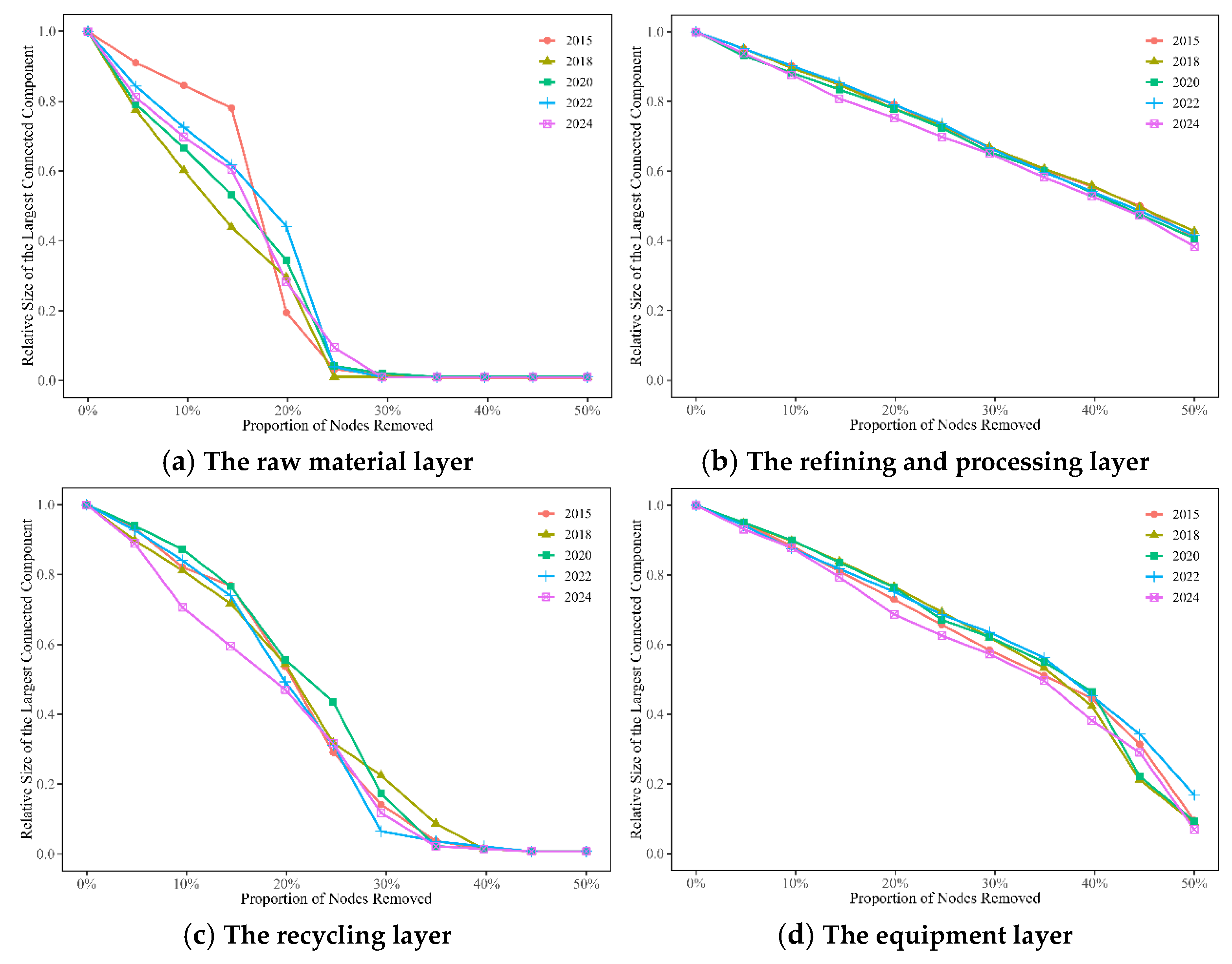
Table A19.
95% Confidence Intervals of Normalized Global Efficiency under Dynamic Random Attacks.
| Industry chain layer | Year | Approximately 10% of nodes removed | Approximately20% of nodes removed | Approximately30% of nodes removed | Approximately40% of nodes removed | Approximately50% of nodes removed |
| The raw material layer | 2015 | [0.756, 0.785] | [0.558, 0.590] | [0.394, 0.426] | [0.253, 0.280] | [0.155, 0.177] |
| 2018 | [0.720, 0.766] | [0.526, 0.570] | [0.362, 0.400] | [0.227, 0.261] | [0.138, 0.163] | |
| 2020 | [0.764, 0.797] | [0.564, 0.602] | [0.394, 0.433] | [0.249, 0.287] | [0.153, 0.180] | |
| 2022 | [0.753, 0.781] | [0.543, 0.576] | [0.394, 0.425] | [0.262, 0.288] | [0.156, 0.177] | |
| 2024 | [0.763, 0.795] | [0.550, 0.587] | [0.392, 0.427] | [0.257, 0.286] | [0.156, 0.177] | |
| The refining and processing layer | 2015 | [0.807, 0.814] | [0.626, 0.634] | [0.481, 0.490] | [0.343, 0.351] | [0.228, 0.235] |
| 2018 | [0.805, 0.812] | [0.620, 0.630] | [0.475, 0.485] | [0.338, 0.347] | [0.226, 0.233] | |
| 2020 | [0.800, 0.811] | [0.616, 0.629] | [0.468, 0.480] | [0.330, 0.340] | [0.219, 0.228] | |
| 2022 | [0.803, 0.814] | [0.620, 0.633] | [0.473, 0.485] | [0.336, 0.348] | [0.225, 0.234] | |
| 2024 | [0.805, 0.817] | [0.623, 0.636] | [0.467, 0.480] | [0.329, 0.342] | [0.221, 0.231] | |
| The recycling layer | 2015 | [0.780, 0.797] | [0.585, 0.603] | [0.435, 0.453] | [0.301, 0.316] | [0.191, 0.204] |
| 2018 | [0.784, 0.800] | [0.596, 0.613] | [0.440, 0.457] | [0.303, 0.320] | [0.194, 0.209] | |
| 2020 | [0.788, 0.803] | [0.600, 0.616] | [0.448, 0.464] | [0.308, 0.323] | [0.197, 0.211] | |
| 2022 | [0.786, 0.802] | [0.585, 0.604] | [0.433, 0.451] | [0.294, 0.311] | [0.192, 0.206] | |
| 2024 | [0.785, 0.804] | [0.581, 0.602] | [0.425, 0.447] | [0.290, 0.309] | [0.183, 0.199] | |
| The equipment layer | 2015 | [0.803, 0.814] | [0.613, 0.628] | [0.459, 0.473] | [0.321, 0.334] | [0.208, 0.218] |
| 2018 | [0.802, 0.811] | [0.616, 0.627] | [0.465, 0.476] | [0.325, 0.337] | [0.216, 0.226] | |
| 2020 | [0.798, 0.809] | [0.610, 0.622] | [0.462, 0.475] | [0.323, 0.335] | [0.211, 0.222] | |
| 2022 | [0.800, 0.812] | [0.615, 0.628] | [0.466, 0.479] | [0.328, 0.340] | [0.217, 0.226] | |
| 2024 | [0.795, 0.807] | [0.609, 0.623] | [0.462, 0.477] | [0.327, 0.341] | [0.215, 0.226] |
Note: The values in square brackets represent the 95% confidence intervals obtained from 100 dynamic random-attack simulations. For concise presentation, representative node removal proportions of 10%, 20%, 30%, 40%, and 50% are reported.
References
- International Energy Agency. The Role of Critical Minerals in Clean Energy Transitions; IEA: Paris, France, 2021; Available online: https://www.iea.org/reports/the-role-of-critical-minerals-in-clean-energy-transitions.
- U.S. Geological Survey. Mineral Commodity Summaries 2025: Copper; U.S. Geological Survey: Reston, VA, USA, 2025; Available online: https://pubs.usgs.gov/periodicals/mcs2025/mcs2025-copper.pdf.
- Chen, X.F.; He, X.Z.; Zhang, Z.F.; Chen, X.; Li, Y. Distribution characteristics and exploration & development pattern of global copper resources and its prospect. China Min. Mag. 2025, 34, 314–323. [Google Scholar] [CrossRef]
- Zhu, Q.; Tang, X.S.; Lei, Y.L.; Sai, S.X.; Huang, S.Z.; Wang, Y.J.; Gu, B.J. Global copper resource industry chain structure evolution and development direction driven by energy transition. Geol. China 2026, 53, 491–506. [Google Scholar] [CrossRef]
- Gereffi, G.; Humphrey, J.; Sturgeon, T. The governance of global value chains. Rev. Int. Political Econ. 2005, 12, 78–104. [Google Scholar] [CrossRef]
- Zhao, G.M.; Guan, M.L.; Geng, Y. Uncovering the dynamic evolution and driving factors of global copper resources trade pattern. J. Nat. Resour. 2026, 41, 1925–1942. [Google Scholar] [CrossRef]
- Li, B.J.; Xing, W.L. Analysis of global trade characteristics of refined copper and its products based on the complex network theory. China Min. Mag. 2021, 30, 57–64. [Google Scholar] [CrossRef]
- Xu, S.T.; Liu, M.L.; Zhu, W.X. Evolution of Global Trade Patterns of Refined Copper and Analysis of China’s Role Based on Complex Networks and Improved Gravity Model. Gold. Sci. Technol. 2025, 33, 1112–1123. [Google Scholar] [CrossRef]
- Dong, X.J.; An, H.G.; Du, Q.J.; Dong, Z.L.; Lu, G. Research on Evolution Characteristics and Response Strategies of Global Trade Network of Scrap Copper Resources. Complex Syst. Complex. Sci. 2022, 19, 104–110. [Google Scholar] [CrossRef]
- Chen, W.; Zhao, X.Q.; Yu, Z.Y. Change of global metallic mineral trade network and its implications. Prog. Geogr. 2025, 44, 1406–1421. [Google Scholar] [CrossRef]
- Ji, Q.D.; Liu, W.D.; Chen, W.; Wang, T. Structure of global copper-containing products trade network based on industrial chain perspective. Sci. Geogr. Sin. 2021, 41, 44–54. [Google Scholar] [CrossRef]
- Zheng, M.G.; Luo, L.W.; Li, Q.; Wen, D.H. Evolution of trade network pattern of copper mineral products in countries along “the Belt and Road” and its influencing factors. China Min. Mag. 2025, 34, 333–345. [Google Scholar] [CrossRef]
- Zheng, M.G.; Zhang, L.X.; Dong, J. Research on resilience evolution of the world copper resources industry chain, supply chain and trade network. Adv. Earth Sci. 2026, 41, 176–191. [Google Scholar] [CrossRef]
- Song, Y.; Bai, W.; Zhang, Y. Resilience assessment of trade network in copper industry chain and the risk resistance capacity of core countries: Based on complex network. Resour. Policy 2024, 92, 105034. [Google Scholar] [CrossRef]
- Wang, S.; Li, J.; Wu, S.; Lei, Y. Research on cascading failures and resilience assessment of multi-layer networks in the global copper supply chain. China Min. Mag. 2026, 35, 185–199. [Google Scholar] [CrossRef]
- Albert, R.; Jeong, H.; Barabási, A.L. Error and attack tolerance of complex networks. Nature 2000, 406, 378–382. [Google Scholar] [CrossRef] [PubMed]
- Crucitti, P.; Latora, V.; Marchiori, M.; Rapisarda, A. Error and attack tolerance of complex networks. Phys. A Stat. Mech. Its Appl. 2004, 340, 388–394. [Google Scholar] [CrossRef]
- Yu, H.; Liu, Z.; Li, Y.J. Key nodes in complex networks identified by multi-attribute decision-making method. Acta Phys. Sin. 2013, 62, 020204. [Google Scholar] [CrossRef]
- Zhu, Q.; Xu, S.Q. Evaluation of Influence of Nodes in Social Network Based on Entropy-weight TOPSIS Method. J. Nanjing Univ. Aeronaut. Astronaut. (Soc. Sci.) 2016, 18, 42–46. [Google Scholar] [CrossRef]
- Blondel, V.D.; Guillaume, J.L.; Lambiotte, R.; Lefebvre, E. Fast Unfolding of communities in Large Networks. J. Stat. Mech. Theory Exp. 2008, 2008, P10008. [Google Scholar] [CrossRef]
- Latora, V.; Marchiori, M. Efficient behavior of small-world networks. Phys. Rev. Lett. 2001, 87, 198701. [Google Scholar] [CrossRef] [PubMed]
- HS commodity codes. https://www.tariffnumber.com/.
- Chen, W.; Zhao, X.Q.; Liu, W.D.; Wuzhati, Y.E.K. The trade network evolution and identification of gateway countries in the Belt and Road region. Acta Geogr. Sin. 2023, 78, 2465–2483. [Google Scholar] [CrossRef]
- Chen, W.; Zhang, H. Characterizing the structural evolution of cereal trade networks in the Belt and Road regions: A network analysis approach. Foods 2022, 11, 1468. [Google Scholar] [CrossRef] [PubMed]
- Federico, L.; Mounim, A.; D’Urso, P.; De Giovanni, L. Complex networks and deep learning for copper flow across countries. Ann. Oper. Res. 2024, 339, 937–963. [Google Scholar] [CrossRef]
Figure 1.
Trends of network topological indicators. (a) Trends in network clustering coefficient (b) Trends in network density (c) Trends in network average degree.
Figure 1.
Trends of network topological indicators. (a) Trends in network clustering coefficient (b) Trends in network density (c) Trends in network average degree.
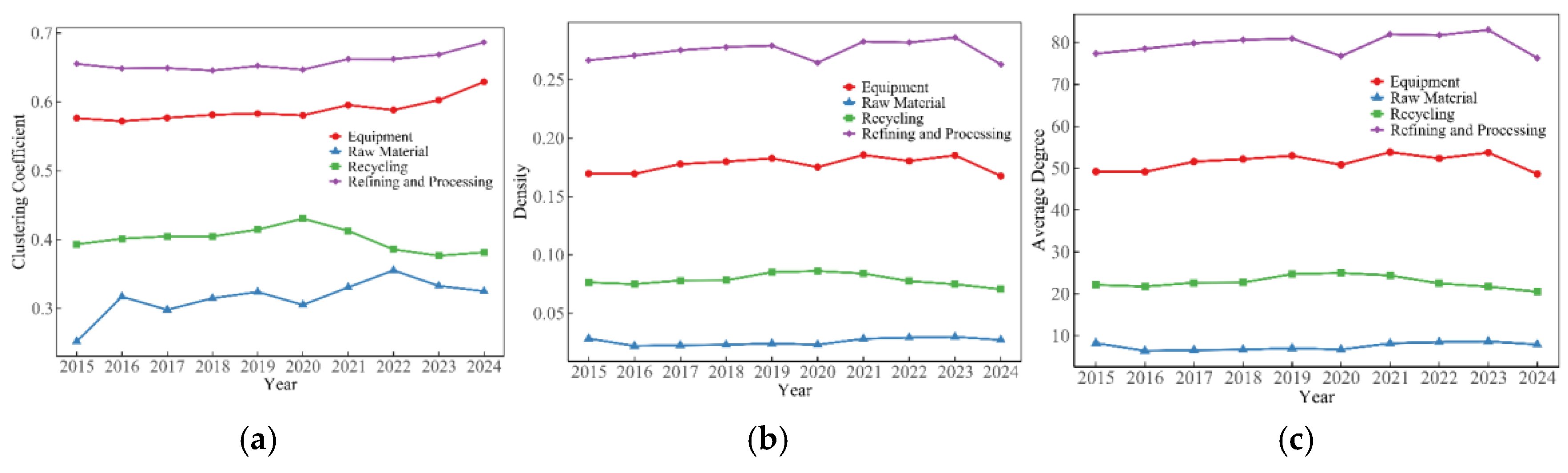
Figure 2.
Spatial visualization of trade flows in the copper raw material layer. This map is based on the standard map with the review number GS(2016)1665 downloaded from the standard map service website of the Ministry of Natural Resources, and the base map has not been modified.
Figure 2.
Spatial visualization of trade flows in the copper raw material layer. This map is based on the standard map with the review number GS(2016)1665 downloaded from the standard map service website of the Ministry of Natural Resources, and the base map has not been modified.
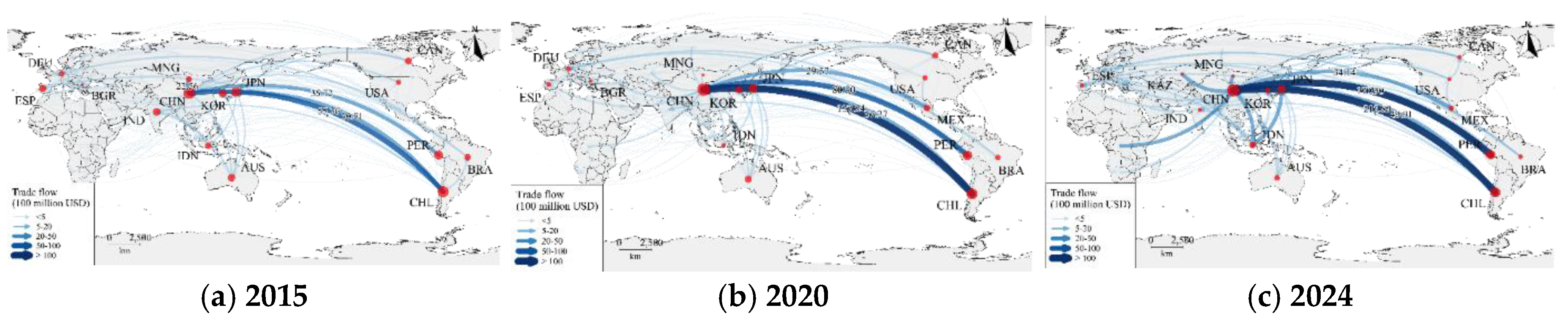
Figure 3.
Spatial visualization of trade flows in the copper refining and processing layer. This map is based on the standard map with the review number GS(2016)1665 downloaded from the standard map service website of the Ministry of Natural Resources, and the base map has not been modified.
Figure 3.
Spatial visualization of trade flows in the copper refining and processing layer. This map is based on the standard map with the review number GS(2016)1665 downloaded from the standard map service website of the Ministry of Natural Resources, and the base map has not been modified.
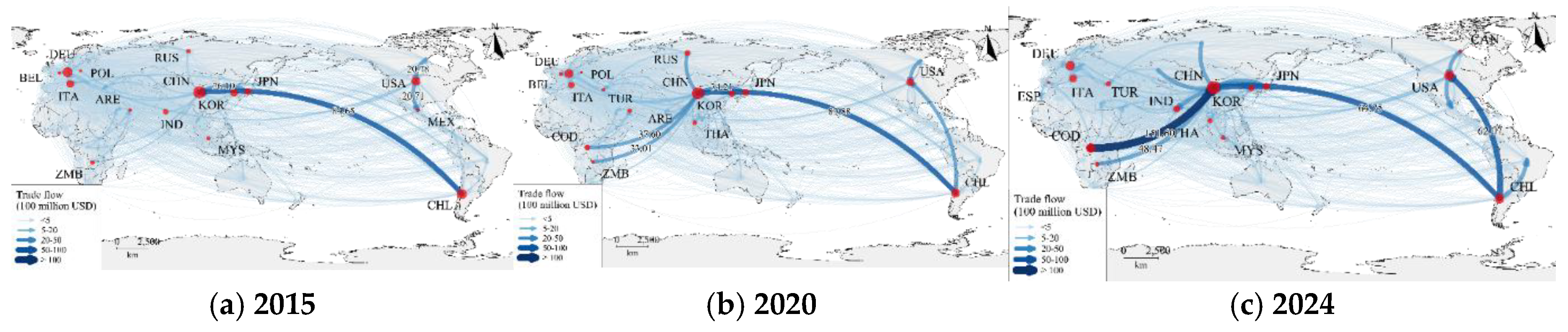
Figure 4.
Spatial visualization of trade flows in the copper recycling layer. This map is based on the standard map with the review number GS(2016)1665 downloaded from the standard map service website of the Ministry of Natural Resources, and the base map has not been modified.
Figure 4.
Spatial visualization of trade flows in the copper recycling layer. This map is based on the standard map with the review number GS(2016)1665 downloaded from the standard map service website of the Ministry of Natural Resources, and the base map has not been modified.
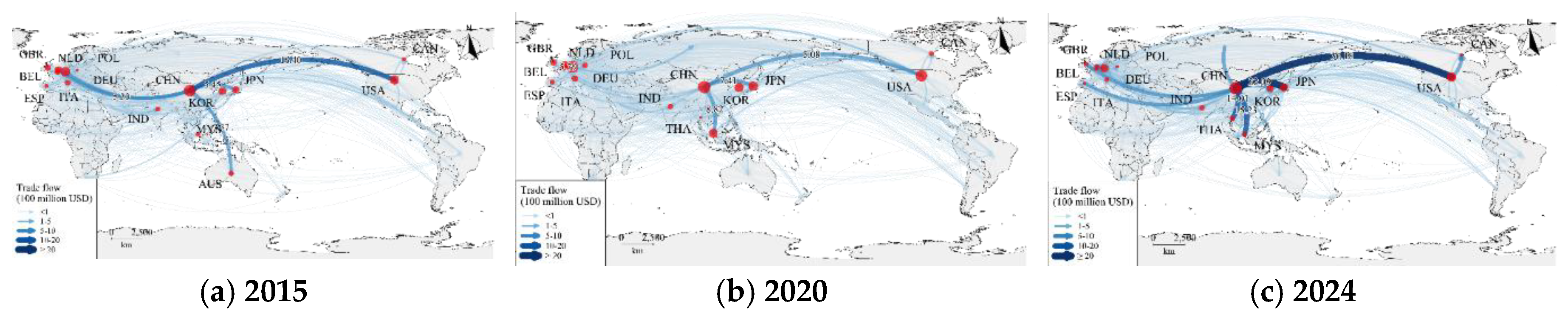
Figure 5.
Spatial visualization of trade flows in the copper equipment layer. This map is based on the standard map with the review number GS(2016)1665 downloaded from the standard map service website of the Ministry of Natural Resources, and the base map has not been modified.
Figure 5.
Spatial visualization of trade flows in the copper equipment layer. This map is based on the standard map with the review number GS(2016)1665 downloaded from the standard map service website of the Ministry of Natural Resources, and the base map has not been modified.
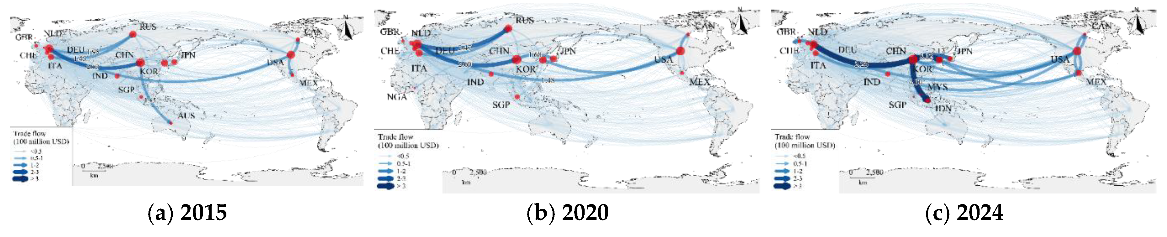
Figure 6.
Evolution of the geographical distribution of trade communities in the copper raw material layer. This map is based on the standard map with the review number GS(2016)1665 downloaded from the standard map service website of the Ministry of Natural Resources, and the base map has not been modified.
Figure 6.
Evolution of the geographical distribution of trade communities in the copper raw material layer. This map is based on the standard map with the review number GS(2016)1665 downloaded from the standard map service website of the Ministry of Natural Resources, and the base map has not been modified.

Figure 7.
Evolution of the geographical distribution of trade communities in the copper refining and processing layer. This map is based on the standard map with the review number GS(2016)1665 downloaded from the standard map service website of the Ministry of Natural Resources, and the base map has not been modified.
Figure 7.
Evolution of the geographical distribution of trade communities in the copper refining and processing layer. This map is based on the standard map with the review number GS(2016)1665 downloaded from the standard map service website of the Ministry of Natural Resources, and the base map has not been modified.
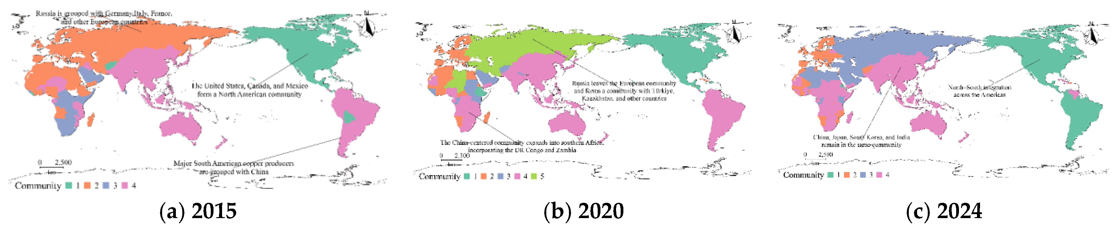
Figure 8.
Evolution of the geographical distribution of trade communities in the copper recycling layer. This map is based on the standard map with the review number GS(2016)1665 downloaded from the standard map service website of the Ministry of Natural Resources, and the base map has not been modified.
Figure 8.
Evolution of the geographical distribution of trade communities in the copper recycling layer. This map is based on the standard map with the review number GS(2016)1665 downloaded from the standard map service website of the Ministry of Natural Resources, and the base map has not been modified.

Figure 9.
Evolution of the geographical distribution of trade communities in the copper equipment layer. This map is based on the standard map with the review number GS(2016)1665 downloaded from the standard map service website of the Ministry of Natural Resources, and the base map has not been modified.
Figure 9.
Evolution of the geographical distribution of trade communities in the copper equipment layer. This map is based on the standard map with the review number GS(2016)1665 downloaded from the standard map service website of the Ministry of Natural Resources, and the base map has not been modified.
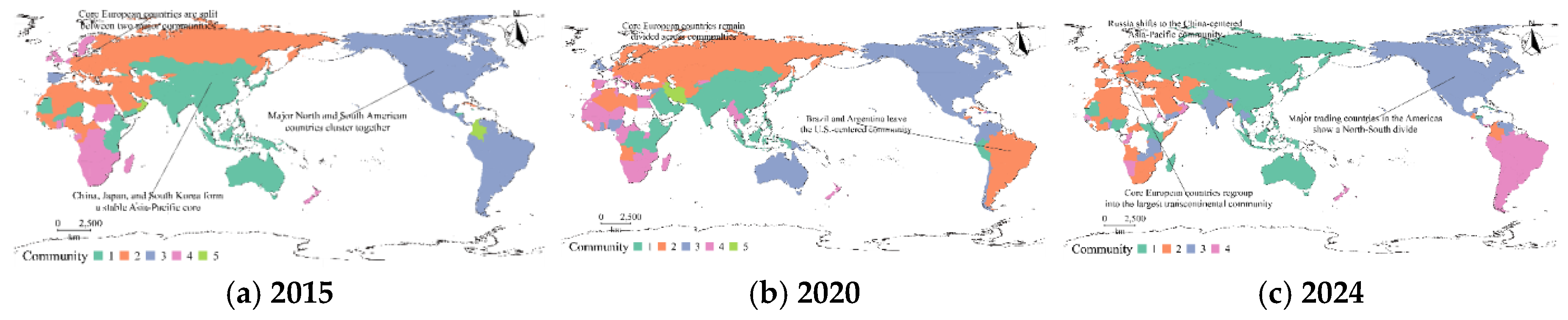
Figure 10.
Results of simulated dynamic attacks on the copper industry chain layers (solid lines indicate deliberate attacks; dashed lines indicate the average results of 100 random attacks).
Figure 10.
Results of simulated dynamic attacks on the copper industry chain layers (solid lines indicate deliberate attacks; dashed lines indicate the average results of 100 random attacks).
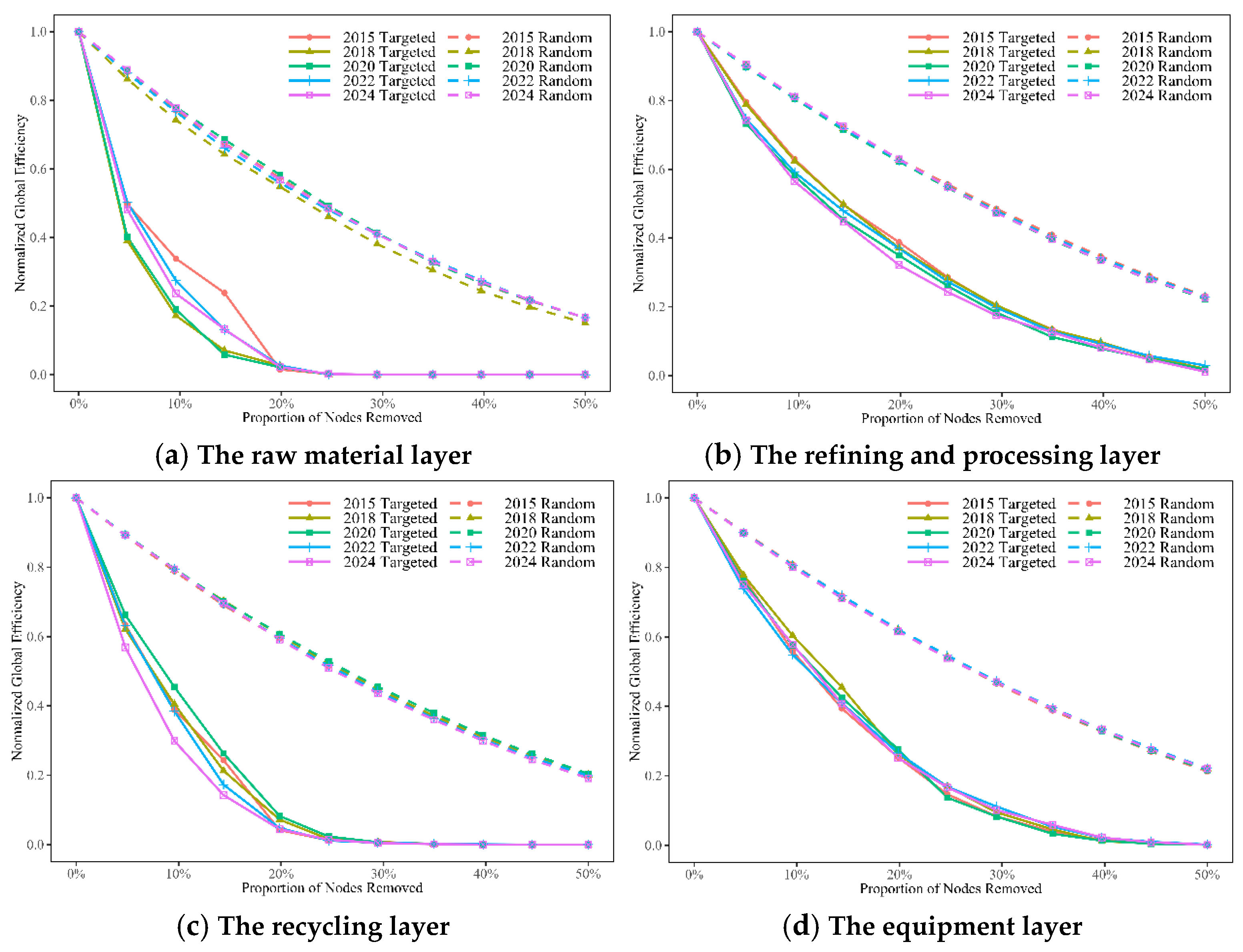
Table 1.
HS codes for each layer of the copper industry chain
| Industry Chain Layer | HS Code | Coverage | Functional Positioning |
| The raw material layer | 260300 | Copper ores and concentrates | Upstream resource supply |
| The refining and processing layer | 74 (excluding 7404) | Copper and articles thereof (excluding copper waste and scrap) | Midstream smelting and processing |
| The recycling layer | 7404 | Copper waste and scrap | Secondary resource recycling |
| The equipment layer | 841989 | Specialized heat-treatment equipment for smelting, rolling, continuous casting, etc. | Proxy for downstream manufacturing capacity |
Table 2.
Indicators of overall network characteristics
| Indicator | Definition | Significance in the trade network | Formula |
| Network density | The ratio of the number of actual edges to the maximum possible number of edges in the network | Measures the intensity of trade connections |
where is the total number of directed edges; is the number of nodes |
| Average degree | The average of the degree values of all nodes | Reflects the average number of trade partners of countries |
where is the number of edges connecting node to other nodes |
| Global clustering coefficient | The proportion of closed triangles among all connected triples in the network | Reflects the grouping and clustering characteristics of trade relationships |
where a “triangle” refers to three nodes that are pairwise connected; a “connected triple” refers to three nodes with at least two edges among them |
Table 3.
Node centrality indicators.
| Indicator | Definition | Significance in the trade network | Formula |
| Weighted in-degree and out-degree | The sum of the weights of all directed edges originating from or pointing to a given node | Weighted in-degree reflects a country’s import scale; weighted out-degree represents its resource supply capacity | ; |
| Weighted degree | The sum of weighted out-degree and weighted in-degree | Reflects a country’s overall trade scale | |
| Betweenness centrality | The number of times a node appears on all shortest paths | Measures a country’s ability to control trade flows by acting as a “bridge” |
where is the total number of shortest paths from node to node ; is the number of those shortest paths that pass through node |
| Eigenvector centrality | The importance of a node depends on the importance of its neighboring nodes | Measures whether a country maintains close and direct ties with important trading partners |
where is the weight of the edge from node to node ; is the eigenvector centrality score of node ; is the largest eigenvalue |
| PageRank | Simulates the probability that a random walker visits a node | Measures the extent to which a country serves as an important trade destination |
where denotes the set of all nodes that point to node ; the damping factor is adopted |
| Entropy-weighted TOPSIS | Based on the multi-attribute decision-making method [18], multiple indicators are integrated to calculate the relative closeness of each node to the positive ideal solution | Integrates multiple indicators to assess the comprehensive influence of each country in the trade network | The core formulas are presented in Eqs. (1)-(3), and the detailed procedures are provided in Appendix B |
Table 4.
Top five countries in terms of node centrality in the trade networks at each layer of the global copper industry chain.
Table 4.
Top five countries in terms of node centrality in the trade networks at each layer of the global copper industry chain.
| Industry chain layer | Year | Rank | Entropy-weighted TOPSIS | Weighted in-degree (Total import trade value) (Unit: 100 million USD) | Weighted out-degree (Total export trade value) (Unit: 100 million USD) |
| The raw material layer | 2015 | 1 | CHN(1) | CHN(186.39) | CHL(139.52) |
| 2 | CHL(0.52) | JPN(78.18) | PER(63.53) | ||
| 3 | PHL(0.40) | IND(38.63) | AUS(40.15) | ||
| 4 | JPN(0.39) | KOR(34.83) | IDN(28.05) | ||
| 5 | IND(0.34) | ESP(23.76) | CAN(26.07) | ||
| 2020 | 1 | CHN(0.99) | CHN(361.27) | CHL(200.17) | |
| 2 | CHL(0.54) | JPN(96.69) | PER(117.99) | ||
| 3 | PER(0.44) | KOR(42.50) | AUS(45.68) | ||
| 4 | ESP(0.37) | DEU(24.22) | MEX(31.13) | ||
| 5 | FIN(0.33) | ESP(17.06) | CAN(28.96) | ||
| 2024 | 1 | CHN(1) | CHN(667.12) | CHL(309.60) | |
| 2 | CHL(0.43) | JPN(133.37) | PER(219.46) | ||
| 3 | PER(0.35) | KOR(50.51) | IDN(81.90) | ||
| 4 | PHL(0.29) | IND(37.08) | AUS(54.60) | ||
| 5 | USA(0.21) | ESP(25.82) | BRA(40.83) | ||
| The refining and processing layer | 2015 | 1 | CHN(1) | CHN(269.60) | CHL(172.42) |
| 2 | DEU(0.52) | USA(77.48) | DEU(90.55) | ||
| 3 | CHL(0.43) | DEU(72.01) | JPN(54.98) | ||
| 4 | USA(0.35) | ITA(56.62) | CHN(48.45) | ||
| 5 | IND(0.26) | KOR(37.75) | ZMB(43.60) | ||
| 2020 | 1 | CHN(1) | CHN(414.49) | CHL(162.14) | |
| 2 | DEU(0.44) | USA(83.47) | DEU(95.18) | ||
| 3 | CHL(0.34) | DEU(72.93) | JPN(73.52) | ||
| 4 | USA(0.25) | ITA(52.19) | COD(63.41) | ||
| 5 | RUS(0.19) | THA(34.80) | CHN(57.21) | ||
| 2024 | 1 | CHN(1) | CHN(523.17) | CHL(211.58) | |
| 2 | DEU(0.43) | USA(161.97) | COD(205.40) | ||
| 3 | COD(0.34) | DEU(96.31) | DEU(119.97) | ||
| 4 | MYS(0.27) | ITA(87.11) | JPN(93.79) | ||
| 5 | USA(0.26) | IND(82.61) | CHN(90.17) | ||
| The recycling layer | 2015 | 1 | CHN(0.85) | CHN(72.59) | USA(26.02) |
| 2 | DEU(0.56) | DEU(24.52) | DEU(17.11) | ||
| 3 | USA(0.41) | KOR(14.40) | NLD(11.47) | ||
| 4 | KOR(0.36) | BEL(8.59) | GBR(10.96) | ||
| 5 | JPN(0.30) | JPN(8.44) | FRA(9.52) | ||
| 2020 | 1 | CHN(0.72) | CHN(39.03) | USA(27.11) | |
| 2 | DEU(0.65) | DEU(25.62) | DEU(14.54) | ||
| 3 | JPN(0.47) | KOR(16.15) | NLD(11.42) | ||
| 4 | USA(0.46) | BEL(13.78) | MYS(10.92) | ||
| 5 | MYS(0.39) | JPN(8.81) | GBR(9.42) | ||
| 2024 | 1 | CHN(0.88) | CHN(170.34) | USA(57.04) | |
| 2 | DEU(0.47) | DEU(30.33) | DEU(25.11) | ||
| 3 | USA(0.38) | KOR(22.42) | JPN(24.04) | ||
| 4 | JPN(0.31) | IND(19.74) | THA(17.85) | ||
| 5 | KOR(0.25) | BEL(18.67) | FRA(17.64) | ||
| The equipment layer |
2015 | 1 | USA(0.82) | RUS(9.51) | DEU(13.00) |
| 2 | DEU(0.79) | CHN(6.91) | CHN(10.21) | ||
| 3 | CHN(0.72) | USA(6.09) | USA(8.86) | ||
| 4 | RUS(0.48) | KOR(3.83) | ITA(6.23) | ||
| 5 | KOR(0.41) | IND(3.21) | KOR(5.29) | ||
| 2020 | 1 | USA(0.85) | RUS(10.10) | DEU(15.54) | |
| 2 | DEU(0.85) | CHN(8.84) | CHN(9.64) | ||
| 3 | CHN(0.83) | USA(7.88) | USA(7.87) | ||
| 4 | RUS(0.45) | KOR(4.37) | ITA(7.23) | ||
| 5 | KOR(0.42) | DEU(3.38) | KOR(5.70) | ||
| 2024 | 1 | CHN(0.89) | CHN(14.55) | CHN(17.59) | |
| 2 | USA(0.78) | USA(13.98) | DEU(17.13) | ||
| 3 | DEU(0.71) | MEX(7.54) | KOR(8.44) | ||
| 4 | KOR(0.39) | IDN(5.20) | USA(8.31) | ||
| 5 | MEX(0.35) | KOR(4.70) | ITA(7.24) |
Table 5.
Major trade communities and core member countries of the copper industry chain layers.
| Industry chain layer | Year | Modularity | Community | Size | Core member countries |
| The raw material layer | 2015 | 0.234 | 1 | 10 | BRA, DEU, ARG, SWE, POL |
| 2 | 13 | CHL, JPN, AUS, IND, KOR, CAN, IDN, PHL | |||
| 3 | 83 | CHN, PER, MNG, USA, MEX, LAO, ERI, KAZ | |||
| 4 | 12 | ESP, BGR, FIN, PRT, GEO, ARM, NAM | |||
| 5 | 5 | COD, ZMB | |||
| 2020 | 0.201 | 1 | 32 | BRA, ESP, DEU, PAN, FIN, SWE, MYS, POL | |
| 2 | 13 | JPN, AUS, KOR, CAN, IDN, IND, PNG, PHL | |||
| 3 | 38 | CHN, CHL, PER, MNG, KAZ, RUS, COD, LAO | |||
| 4 | 10 | BGR, ARM, GEO, NAM, TUR, SRB | |||
| 5 | 3 | MEX, USA | |||
| 2024 | 0.208 | 1 | 40 | BRA, ESP, DEU, FIN, TUR, SWE, NAM, POL | |
| 2 | 16 | JPN, IDN, AUS, KOR, CAN, IND, PHL, PNG | |||
| 3 | 38 | CHN, CHL, PER, MNG, KAZ, COD, SRB, RUS | |||
| 4 | 4 | UZB | |||
| 5 | 8 | MEX, USA | |||
| The refining and processing layer | 2015 | 0.378 | 1 | 14 | USA, MEX, CAN |
| 2 | 65 | DEU, ITA, FRA, BEL, RUS, POL, TUR, ESP | |||
| 3 | 24 | ZMB, ARE, COD, SAU | |||
| 4 | 41 | CHN, CHL, KOR, JPN, IND, MYS, AUS, THA | |||
| 2020 | 0.366 | 1 | 12 | USA, MEX, CAN | |
| 2 | 47 | DEU, ITA, BEL, FRA, POL, ESP, BGR, AUT | |||
| 3 | 15 | ARE, COG | |||
| 4 | 48 | CHN, CHL, JPN, KOR, COD, THA, ZMB, IND | |||
| 5 | 23 | RUS, TUR, KAZ | |||
| 2024 | 0.409 | 1 | 18 | USA, CHL, CAN, MEX, PER, BRA | |
| 2 | 45 | DEU, ITA, BEL, ESP, FRA, POL, BGR, SWE | |||
| 3 | 28 | TUR, KAZ, RUS, ARE, SAU, EGY | |||
| 4 | 55 | CHN, COD, JPN, IND, KOR, THA, MYS, ZM | |||
| The recycling layer | 2015 | 0.329 | 1 | 40 | DEU, NLD, FRA, ITA, BEL, ESP, POL, AUT |
| 2 | 52 | KOR, JPN, IND, SAU, ARE, PHL, ZAF, THA | |||
| 3 | 25 | CHN, USA, GBR, AUS, MYS, CAN, MEX, COL | |||
| 4 | 12 | BGR, GRC, ROU | |||
| 5 | 5 | RUS | |||
| 2020 | 0.364 | 1 | 47 | DEU, BEL, NLD, ITA, FRA, GBR, ESP, POL | |
| 2 | 38 | IND, SAU, ARE, BGR, GRC, TUR | |||
| 3 | 48 | CHN, USA, JPN, KOR, MYS, CAN, THA, MEX | |||
| 2024 | 0.339 | 1 | 35 | DEU, BEL, ITA, FRA, NLD, ESP, POL, AUT | |
| 2 | 34 | IND, GBR, SAU, COL, BRA | |||
| 3 | 46 | CHN, USA, JPN, KOR, THA, MYS, CAN, MEX | |||
| 4 | 19 | BGR, GRC, TUR | |||
| The equipment layer | 2015 | 0.178 | 1 | 40 | CHN, KOR, JPN, IND, SGP, AUS, MYS, PAK |
| 2 | 50 | DEU, RUS, ITA, FRA, CHE, TUR, AUT, POL | |||
| 3 | 20 | USA, CAN, MEX, ESP, BRA | |||
| 4 | 25 | GBR, NLD, SWE, BEL, DNK | |||
| 5 | 2 | OMN, COL | |||
| 2020 | 0.190 | 1 | 31 | CHN, KOR, JPN, IND, SGP, IDN, VNM, MYS | |
| 2 | 44 | DEU, RUS, CHE, TUR, AUT, POL, DNK, SWE | |||
| 3 | 25 | USA, NLD, MEX, CAN, GBR, NGA, AUS | |||
| 4 | 38 | ITA, FRA, ESP, BEL, THA | |||
| 5 | 2 | IRN, AZE | |||
| 2024 | 0.199 | 1 | 31 | CHN, KOR, JPN, IDN, SGP, MYS, AUT, AUS | |
| 2 | 62 | DEU, ITA, NLD, GBR, CHE, FRA, SWE, TUR | |||
| 3 | 19 | USA, MEX, IND, CAN, THA, SVK | |||
| 4 | 19 | BRA, DNK, ARG, OMN |
Note: Community numbers missing in certain years correspond to countries with extremely small trade volumes and are therefore not listed in the table.
Table 6.
Results of simulated dynamic deliberate attacks
| Industry chain layer | Year | AUC | half-life | collapse threshold |
| The raw material layer | 2015 | 0.077 | 4.8% | 17.8% |
| 2018 | 0.056 | 3.9% | 13.0% | |
| 2020 | 0.057 | 4.0% | 12.9% | |
| 2022 | 0.069 | 4.8% | 16.0% | |
| 2024 | 0.067 | 4.6% | 16.0% | |
| The refining and processing layer | 2015 | 0.177 | 14.3% | 38.8% |
| 2018 | 0.175 | 14.3% | 39.4% | |
| 2020 | 0.163 | 12.6% | 36.7% | |
| 2022 | 0.170 | 13.5% | 38.8% | |
| 2024 | 0.160 | 12.3% | 37.8% | |
| The recycling layer | 2015 | 0.089 | 7.4% | 18.3% |
| 2018 | 0.089 | 7.5% | 18.8% | |
| 2020 | 0.097 | 8.5% | 19.3% | |
| 2022 | 0.085 | 7.3% | 17.6% | |
| 2024 | 0.076 | 6.0% | 16.8% | |
| The equipment layer | 2015 | 0.136 | 11.3% | 28.2% |
| 2018 | 0.143 | 12.9% | 29.1% | |
| 2020 | 0.138 | 12.0% | 28.0% | |
| 2022 | 0.139 | 11.3% | 30.6% | |
| 2024 | 0.139 | 11.8% | 29.6% |
Disclaimer/Publisher’s Note: The statements, opinions and data contained in all publications are solely those of the individual author(s) and contributor(s) and not of MDPI and/or the editor(s). MDPI and/or the editor(s) disclaim responsibility for any injury to people or property resulting from any ideas, methods, instructions or products referred to in the content. |
© 2026 by the authors. Licensee MDPI, Basel, Switzerland. This article is an open access article distributed under the terms and conditions of the Creative Commons Attribution (CC BY) license (http://creativecommons.org/licenses/by/4.0/).
Copyright: This open access article is published under a Creative Commons CC BY 4.0 license, which permit the free download, distribution, and reuse, provided that the author and preprint are cited in any reuse.