

Submitted:
14 September 2026
Posted:
15 September 2026
You are already at the latest version
Abstract
The Vere River basin in Tbilisi, Georgia, experienced a major cascading landslide-flood disaster in June 2015, emphasizing the need to evaluate the present stability of slopes adjacent to the former source area. This study combines Small-Baseline InSAR (SBAS), RTK-UAV photogrammetry, COSI-Corr image correlation and LS-RAPID numerical modelling to investigate whether the slope remains active and how it responds to changing pore-pressure conditions. Analysis of 109 ascending Sentinel-1 acquisitions acquired between April 2022 and October 2025 revealed persistent positive line-of-sight deformation across the investigated slope. Independent UAV/COSI-Corr analysis identified horizontal displacements of approximately 0.05-0.09 m over 149 days, exceeding the empirical relative displacement detection threshold of 0.0235 m. The measured displacement direction broadly follows the downslope and structural orientation, although its angular offset suggests that the movement is influenced by a combination of topography, bedding, fractures, and heterogeneous slope materials rather than a single planar control. LS-RAPID simulations further showed a nonlinear response to increasing prescribed pore-pressure ratio. Together, the observations indicate that the slope has not fully stabilized after the 2015 event and continues to undergo slow deformation while remaining sensitive to hydrological conditions. This is particularly important for Tbilisi because renewed slope instability in the Vere valley could interact with the confined river corridor and urban infrastructure, increasing the potential for cascading impacts.
Keywords:
SBAS InSAR
; UAV photogrammetry
; slope deformation
; slope stability
; numerical modelling
; Vere River basin
1. Introduction
Rainfall-induced landslides are among the most recurrent geohazards in mountainous urban catchments, where steep terrain, weathered geological materials and increasing exposure of infrastructure and population amplify their potential risks and consequences. Slope failure is generally controlled by the combination of hydrological, geological, and time-dependent mechanical processes rather than by rainfall intensity alone. While the antecedent precipitation determines the initial moisture and groundwater conditions within a slope, subsequent rainfall infiltration can increase water pore pressure and decrease shear resistance along pre-existing discontinuities or potential sliding surfaces [1,2]. The resulting response is strongly conditioned by lithology, degree of weathering, permeability contrasts, and geological structure, particularly the orientation and persistence of bedding, joints, and faults relative to the slope. Repeated wetting and weathering can precondition creep and progressive deformation with shear-surface development to accumulate over time and leading to accelerating movement and failure [3]. Earthquakes can be another major trigger of landslide activity, but their importance depends on the local seismotectonic and geological setting.
Satellite InSAR (Interferometric Synthetic Aperture Radar) is widely used for detecting and monitoring slow-moving landslides because it provides repeated, large-area measurements of surface deformation [4,5]. While DInSAR (Differential Interferometric Synthetic Aperture Radar) captures displacement between acquisitions, multi-temporal approaches such as PSI (Persistent Scatterer Interferometry Synthetic Aperture Radar) and SBAS (Small Baseline Subset) improve deformation time-series analysis by reducing atmospheric effects and decorrelation [4,6]. However, their performance can be limited in mountainous terrain, because dense vegetation reduces coherence and steep slopes cause shadowing and unfavorable viewing geometries [5,7]. Should be noted that the conventional InSAR measures only the line-of-sight (LOS) component of displacement, which can complicate interpretation of complex landslide motion [5,7], therefore while PSI and SBAS are highly effective for regional and long-term monitoring, additional techniques are often required for detailed analysis in vegetated and high-relief environments.
UAV (Unmanned Aerial Vehicle) -based Structure-from-Motion (SfM) photogrammetry can provide centimetre-scale topography and imagery, which can be used for detailed monitoring of landslide deformation. These multi-temporal images and their correlation can quantify the magnitude and direction of surface displacement [8,9]. However, their accuracy strongly depends on image georeferencing and acquisition geometry and this effects reliability of image matching and displacement estimates [8,10]. Inadequate camera calibration and near-parallel image geometry are another source of potential bias in terms of estimating topographic change using UAV-SfM models [10,11].
Physically based and numerical models are increasingly used to investigate the mechanisms controlling slope instability to complement these observation-based techniques. It helps to translate measured deformation into process-based interpretations. Such approaches can simulate rainfall infiltration, pore-pressure evolution, strength reduction, and as a result, slope deformation or failure. Finite-element methods, discrete-element methods, and integrated models such as LS-RAPID are commonly applied to represent different stages of landslide initiation and motion under hydrological forcing [9,12].
Despite these advances, an important gap remains between deformation monitoring and process-based assessment of slope stability. While remote sensing techniques can detect and quantify surface displacement, they cannot determine failure initiation and its process. At the same time, numerical models can include rainfall infiltration, pore-pressure evolution and strength degradation but remain sensitive to uncertainties related to subsurface geometry and material parameters. Relatively few studies integrate SAR analyses with repeated RTK-UAV observations, field and geophysical constraints and numerical modelling of rainfall-induced deformation and failure susceptibility in densely populated urban catchments. This gap is particularly relevant for the Vere River catchment in Tbilisi (Figure 1), where the 13-14 June 2015 disaster developed as a cascading hydro-geomorphic event involving extreme rainfall, hillslope failure, debris entrainment and hydraulic blockage within a densely urbanized valley.
This study aims to assess whether the slopes near the 2015 landslide area are currently stable or show evidence of ongoing instability. We examine whether measurable surface deformation is present using InSAR, RTK-UAV observations, image correlation and evaluate whether the observed conditions are consistent with potential slope movement.
The 2015 Vere River catastrophe represented a cascading flood - landslide - debris flow - blockage sequence in which several processes interacted over a short time (Figure 2). Antecedent flooding on 4 June likely preconditioned the channel by increasing sediment and wood debris availability, while about 160 mm of rainfall of 13-14 June [10] generated rapid runoff across the steep Vere catchment. However, the most severe urban impacts were strongly controlled by anthropogenic modification of the lower valley, particularly the blockage of the tunnel system by debris and truck. The temporary impoundment and sudden release of water transformed the upstream flood into a much larger downstream surge, producing an estimated peak discharge of 468 m³/s [11]. As a result, dozens of people died, roads, zoo and other infrastructure was damaged or destroyed. This sequence highlights the importance of treating the 2015 event not simply as an extreme hydrological flood, but as a multi-process cascading hazard amplified by confined valley morphology and urban infrastructure that makes future hazard assessment extremely challenging.
According to reports (e.g. Bennett, et. al., 2015) and aerial/satellite surveys, there are many small landslides just east of the main landslide, some of which were activated at the same time as the major event.
In this study, we use satellite radar, UAV photogrammetry, and landslide simulation techniques to assess the current stability of the slopes adjacent to the main landslide and simulate the potential development of a landslide on the selected slope. We combine satellite radar interferometry, UAV-based photogrammetry, GNSS-supported field measurements and landslide simulation techniques.
The purpose of this study is therefore to determine whether slopes adjacent to the 2015 landslide source area remain active or potentially unstable. By integrating rainfall, deformation, high resolution topographic and simulation data, in a condition that downstream area is still undergoing an intense infrastructure development, this work aims to improve understanding of post disaster slope instability in a highly urbanized mountain catchment and to support future hazard assessment for the Vere gorge.
2. Study Area
2.1. Vere River Basin and Disasters
The Vere River is a short (~50 km) river flowing from the west into the Mtkvari (Kura) River in Tbilisi, draining a small (~200 km²), steep, and elongated basin (Figure 1). Its mountainous terrain, erodible soils, and narrow gorge produce rapid runoff, high flow velocities, and significant sediment transport during storms. The river is mainly rain-fed, with low base flow but sharp discharge peaks, making it highly prone to flash flooding and debris flows. Urbanization in downtown Tbilisi, through channelization and infrastructure development into the hazard impact area, further amplifies flood and debris flow risk, as demonstrated by the 2015 Tbilisi flood/debris-flow.
The Vere River basin exhibits morphometric characteristics indicative of an elongated and steep mountainous catchment. The total basin area is approximately 200 km², with a main channel length of 50 km and a sinuosity index of 1.43, suggesting moderate meandering influenced by topographic and structural controls [13]. The mean annual discharge of the river is 0.98 m³/s. Prior to the most recent extreme hydrological event, the highest recorded peak discharge was 259 m³/s, observed on July 5, 1960. The absolute maximum discharge was recorded during the flood event of June 13-14, 2015, reaching 468 m³/s [11].
The elongation ratio (Re) of 0.55 confirms that the basin has elongated shape, which typically is associated with delayed runoff and reduced flood peaks [14]. However, in the case of the Vere basin, this theoretical implication is counterbalanced by other dominant factors, including its high basin relief of 1283 m, steep slopes and rapid surface runoff dynamics. These characteristics, combined with intense convective precipitation events and limited infiltration capacity, create conditions highly favorable for flash flooding, as historically observed during the catastrophic 2015 Tbilisi flood and other events [11].
The basin perimeter is 105 km, and the basin length is 28 km. The drainage density, calculated as the total stream length per unit area, is relatively low at 0.52 km-1, typically reflecting either permeable lithology or vegetated land cover.
The 2015 Vere River catastrophe represented a cascading flood - landslide - debris flow - blockage sequence in which several processes interacted over a short time. Antecedent flooding on 4 June likely preconditioned the channel by increasing sediment and wood debris availability, while about 160 mm of rainfall of 13-14 June [10] generated rapid runoff across the steep Vere catchment. However, the most severe urban impacts were strongly controlled by anthropogenic modification of the lower valley, particularly the blockage of the tunnel system by debris and truck. The temporary impoundment and sudden release of water transformed the upstream flood into a much larger downstream surge, producing an estimated peak discharge of 468 m³/s [11]. As a result, dozens of people died, roads, zoo and other infrastructure was damaged or destroyed. This sequence highlights the importance of treating the 2015 event not simply as an extreme hydrological flood, but as a multi-process cascading hazard amplified by confined valley morphology and urban infrastructure that makes future hazard assessment extremely challenging.
Archival records of 20th century show that flooding in the Vere River basin was a recurrent hazard, with major events recorded on 11-12 June 1924, 10 May 1940, 4 July 1960, and 7 June 1972. The 1940 flood caused severe damage, affecting houses, many other types of infrastructure, and nearly destroying the Tbilisi Zoo. The 1960 flood again heavily damaged the zoo. Another destructive flood occurred in 1972, when ‘heavy’ rainfall affected more than 1600 families, caused 10 fatalities, damaged infrastructure again.
2.2. Geological Settings
The Vere River basin is located within a structurally complex zone west to capital city Tbilisi where folded Cenozoic sedimentary rocks are dissected by a relatively short but steep mountain river system. The basin extends from the highlands to the Mtkvari River in central Tbilisi and is characterized by a strong altitudinal gradient, narrow valleys, deeply incised tributaries, and locally oversteepened slopes. This geomorphic setting creates favorable conditions for rapid runoff generation, slope failures, debris flow initiation, and downstream sediment transfer. The bedrock geology of the basin is dominated by Paleogene sedimentary units, including Eocene-Oligocene sandstones, marls, argillites, and localized conglomeratic beds. These lithologies are heterogeneous and shows strong contrasts in permeability, weathering and shear strength. Sandstone layers commonly form relatively competent beds, whereas argillites, marls, and clay-rich horizons are more prone to weathering and deformation. Such lithological alternation promotes the development of failure-prone surfaces, particularly where clay rich beds dip in the same general direction as the hillslope. This relationship reduces the effective resistance of the rock mass and can favor sliding along weak stratigraphic horizons. The presence of fractures and discontinuities within the layered bedrock enhances rainfall infiltration which increases weathering intensity and reducing the mechanical resistance of the slope material (Figure 3).
The investigated slope is located within the upper Tskneti-Akhaldaba landslide complex, close to the source area of the 2015 failure on the southern flank of the Vere River valley. The regional hillslope is characterized by steep north-facing terrain, with locally reported inclinations of 30-45°. The bedrock is represented predominantly of Upper Eocene and Oligocene sedimentary sequences. The Oligocene layers are built mainly by thinly bedded argillites with sandstone interlayers, whereas the Upper Eocene succession contains thicker sandstone and locally conglomerate beds interbedded with argillites. Bedding generally dips north-northwestward at approximately 30-50° and is broadly subparallel to the hillslope. The rock mass is strongly fractured, locally faulted and weathered; Weak and strongly weathered clay-rich bedding horizons provide mechanically plausible surfaces for translational displacement. Bedrock is covered by colluvial deposits, with thickness reaching approximately several centimeters up to 1-2 m or more. The slope is forested.
Hydrogeological observations indicate that colluvial materials readily receive infiltrating precipitation, but clay-rich and less-permeable bedrock horizons can restrict downward drainage. At the same time fractures, joints and fault-related discontinuities within the bedrock can act as preferential flow pathways that supports rapid and relatively deep infiltration of rainfall water. Groundwater flow is consequently influenced by bedding and fractures and may become concentrated along the slope and near the contact between surficial deposits and underlying bedrock. Small spring and temporary groundwater occurrence have been reported from this area. Previous studies therefore proposed rainfall-induced groundwater rise and associated pore-pressure increase as important controls on the 2015 instability [15].
2.3. Climate and Rainfall
The Vere River basin stretches from its headwaters at 1672 m a.s.l. to its confluence at 389 m a.s.l., covering an elevation range of 1283 m over a 28 km basin length. This pronounced elevation gradient plays a major role in shaping the basin’s thermal and precipitation regimes, creating vertical climatic zonation typical of mountainous environments.
To characterize the climate, data from two meteorological stations TSU Hydrometeorological Lab (460 m) and Kojori (1340 m) have been used (see the locations at the Figure 1). These stations can be representatives of the lower and upper sections of the basin, respectively.
The basin experiences a temperate climate with strong seasonality, where temperatures increase from January (coldest) to July - August (warmest). There is a clear altitudinal temperature lapse rate, with Kojori being on average ~4.5°C cooler than the TSU Lab station (Table 1).
The upper basin (Kojori) receives ~74% more precipitation than the lower basin, which is consistent with orographic factors and moisture interception by the surrounding ridges.
Peak precipitation occurs during April, May and June. This pattern can be influenced by spring cyclonic activity and convective rainfall. Summer (June - August) precipitation is still significant but decreases toward July and August, indicating potential for flash floods due to convective storms. Wettest months are May (Kojori: 125 mm) and April (Kojori: 91 mm) and driest months are January (TSU: 15 mm) and December (TSU: 17 mm) Figure 4.
Seasonality Index (SI) [16], which measures the degree of precipitation seasonality (where SI > 0.2 indicates moderate to strong seasonality), for TSU Hydrometeorological Lab (460 m) is 0.37 and for Kojori (1340 m) is 0.28. This, along with monthly distribution, suggests that both locations in the Vere River basin experience marked precipitation seasonality, with more concentrated rainfall during spring and early summer. This has important implications for runoff generation, erosion and flash flood potential.
The combination of high spring precipitation and snowmelt from upper elevations increases the likelihood of spring floods and flash floods, especially given the basin's steep relief and elongated shape. Convective summer storms (despite slightly lower monthly totals) may cause localized intense rainfall, which is a common trigger for flash floods, particularly in lower basin areas like Tbilisi. Snow accumulation and melt dynamics in higher altitudes also contribute significantly to seasonal runoff patterns.
The Vere River basin displays a vertical climatic gradient typical of mountainous catchments, with cooler, wetter conditions at higher elevations. The seasonal thermal and precipitation regime, characterized by spring maximum and summer heat, shapes the basin's hydrology and contributes to natural hazards, especially in the context of steep topography and urbanized lower sections. These factors amplify the basin's vulnerability to flash floods and landslides/mudflows, particularly from intense spring or summer precipitation events.
3. Materials and Methods
3.1. Small-Baseline InSAR Time-Series Analyses
Ascending Sentinel 1 IW Synthetic Aperture Radar (SAR) images were use to asses line-of-sight (LOS) ground deformation in western Tbilisi area. C-band SAR observations provided by Sentinel 1 are suitable for surface deformation interferometric monitoring [17]. Interferometric products were generated using the Alaska Satellite Facility (ASF) Hybrid Pluggable Processing Pipeline (HyP3). The analysis used 109 Sentinel-1 ascending acquisitions from 2 April 2022 to 31 October 2025, burst ID was 371837, sub-swath - IW1, and VV polarization. HyP3 Burst InSAR products were generated using the 5 × 1 multilooking option, corresponding to a nominal pixel spacing of 20 m and an effective spatial resolution of approximately 40 m; the water-mask option was enabled during processing.
A small-baseline InSAR time-series approach was used to reduce temporal and geometric decorrelation and to reconstruct the LOS displacement from a dense interferometric network. The general concept is according the Small Baseline Subset (SBAS) framework, in which interferograms with relatively short temporal and perpendicular baselines are combined to estimate displacement through network inversion [4,18]. Time-series approaches provides greater temporal redundancy than individual differential interferograms and reduces errors from atmospheric, topographic, and phase-unwrapping [4,5,19,20]. In this approach, the workflow can more be called as a variance-weighted small-baseline InSAR time-series inversion, rather than a strict implementation of the original SBAS formulation of Berardino et al. (2002).
The analysis covered the period from 2 April 2022 to 31 October 2025 and used 109 Sentinel 1 acquisitions. A total of 253 differential interferograms were generated (list is provided as Supplementary material 1). The interferometric network was limited to 48 days of a maximum temporal baseline and a maximum perpendicular baseline of 100 m. The use of short temporal and orbital baselines was intended to limit loss of interferometric coherence associated with temporal surface changes and geometric decorrelation.
The HyP3 products were imported into MintPy v1.6.4, which is an open-source framework for InSAR time-series analysis [5,20]. The interferometric network was inverted using a variance-weighted least-squares solution (weightFunc = var) with minimum-norm velocity estimation. No coherence mask was used during the network inversion itself, allowing displacement estimates to be calculated independently of the temporal-coherence threshold subsequently used for quality control. This approach is consistent with the MintPy small-baseline framework, where interferometric observations are inverted jointly to retrieve the displacement time series before deterministic error components are corrected [20].
MintPy was used in to assess the phase-unwrapping errors and correct them the phase-closure method. For three acquisitions t1, t2 and t3 correctly unwrapped interferometric phases should satisfy the closure relation:
where is phase difference between acquisition 1 and acquisition 2, is phase difference between acquisition 2 and acquisition 3 and is phase difference between acquisition 1 and acquisition 3. If the interferograms are correctly unwrapped, the phase change from 1 to 2 plus the phase the change from 2 to 3 should equal the phase change directly from 1 to 3. Here deviations by integer multiples of 2π indicates potential phase-unwrapping ambiguities. The final interferometric network contained 205 independent closure triplets. They provided sufficient redundancy for closure-based identification and correction of integer phase ambiguities [20].
Atmospheric effects can impose phase delays, particularly in areas of high relief and may be misinterpreted as deformation if not corrected. Reanalysis-based atmospheric models estimate the radar propagation delay from atmospheric pressure, temperature, and humidity fields and provide an independent means of reducing topography-correlated tropospheric artifacts. Therefore, after the network inversion, tropospheric phase delays were corrected using the ERA5 atmospheric reanalysis through the PyAPS implementation in MintPy [21].
Another source of possible inaccuracies is residual topographic phase errors in the reference DEM, which was estimated and removed using the time-domain DEM-related error correction included in MintPy. This procedure uses the relationship between residual topographic phase and the changing perpendicular-baseline geometry through time and estimates the DEM-error contribution pixel-wise after time-series inversion [22]. Pixel-wise incidence-angle and slant-range geometry were used in the correction. Additionally, a second-order temporal polynomial applied internally during DEM-error estimation.
The residual root-mean-square (RMS) time series was used to perform temporal quality control. The acquisition with the minimum residual RMS, which is 24 August 2022, was adopted as the temporal reference date. The minimum RMS was 0.0031 m. No acquisition exceeded the MintPy outlier threshold of three times the median-based RMS criterion (0.0357 m). Therefore, all 109 acquisitions were kept for the final velocity estimation. Afterwards, to estimate the mean LOS velocity over the 2022-2025 observation period, a linear displacement model was fitted independently at each valid pixel.
Because only ascending Sentinel 1 observations were used, the estimated LOS velocity represents a projection of the true three-dimensional displacement vector and cannot be interpreted directly as vertical or downslope motion. As a result, the InSAR results can be interpreted primarily in terms of the spatial distribution and relative magnitude of coherent LOS deformation.
3.2. Photogrammetric Modelling and Validation Using GNSS
Drone-based photogrammetric surveys and modeling are increasingly employed for monitoring surface displacement (e.g., [23,24]). Following the Small-Baseline InSAR analysis, the study area was surveyed four times using an RTK-enabled Autel Evo II Pro drone. This drone is equipped with a 1-inch CMOS, 20-megapixel camera capable of capturing images at a resolution of 5472 × 3648 pixels. All surveys were conducted using preplanned flight missions, ensuring 80% frontal overlap and 70% side overlap between consecutive images to maximize photogrammetric quality.
The first survey covered the entire study area that was selected based on InSAR analyses, resulting in the acquisition of 598 images. Its primary objective was to obtain a comprehensive overview of the area and to evaluate the performance of the photogrammetric workflow.
The subsequent three surveys focused on a smaller zone that met two criteria:
- (a)
- the area included LOS deformation as detected by InSAR analysis, and
- (b)
- the surface was characterized by hard, non-vegetated material, such as asphalt, which is favorable for photogrammetric matching.
All the next three missions were planned to capture images with 80% frontal overlap and 70% side overlap from a flight altitude of 60 meters, resulting in 97 images per survey under optimal conditions.
The second survey, conducted on 28 June 2024, was affected by strong winds, which limited the drone's ability to complete the planned flight path. As a result, only 49 images were captured, and the required coverage was not achieved. Therefore, this dataset was excluded from further analysis.
The third (07 October 2024) and fourth (05 March 2025) surveys were conducted as planned, with full coverage and image acquisition according to the predefined flight parameters (Figure 5).
In PIX4Dmatic, GCP-independent, direct-georeferencing workflow was used to conduct Photogrammetric processing. The onboard GNSS/RTK-derived image positions were retained as exterior-position observations during photogrammetric adjustment. No ground control points were introduced into the processing. although independent, GCP-based validation remains important for identifying systematic errors, in this case, just direct georeferencing, using centimetre-level onboard RTK positioning has been used [25,26,27].
Image matching was done primarily by automatically generated tie points, supported by manually identified tie points (MTPs). Seven MTPs were used for the October 2024 reconstruction and eight for the March 2025 reconstruction. These points were distributed longitudinally throughout the survey corridor and were identified in multiple overlapping images. Should be noted that these tie points do not include externally surveyed coordinates and therefore they are not GCPs. The October reconstruction included 241672 automatic tie points, with a median of 7503 matches per calibrated image. The MTPs had an RMS reprojection error of approximately 0.7 pixels. The March reconstruction included 265591 automatic tie points, with a median of 7322 matches per calibrated image. The MTP RMS reprojection error of 0.9 pixels.
Camera internal parameters were optimized simultaneously with the tie-point network and the resulting self-calibration was highly consistent between the two independently processed surveys. The optimized focal lengths were 4227.5 pixels in October 2024 and 4248.0 pixels in March 2025, differing by approximately 0.48%, while the optimized principal-point coordinates and radial-distortion parameters were similarly consistent between epochs. The relative change between the initial and optimized internal camera parameters reported by PIX4Dmatic was 0.07% for October and 0.56% for March. This type of inter-epoch consistency is relevant, because systematic broad-scale deformation in SfM models may arise from correlations between camera self-calibration parameters and weak, predominantly nadir image-network geometry [7,28].
Two ground GNSS points were surveyed independently for each acquisition epoch and deliberately excluded from the photogrammetric adjustment. These observations are referred to here as independent checkpoints (CPs) rather than GCPs. Field observations of CPs were carried out using a Topcon HiPer SR RTK receiver and antenna, mounted on a tripod with an optical tribrach. The tribrach, equipped with a precision optical plummet and laser pointer. While the benchmarks used in this study were not officially classified as geodetic, they were designed in accordance with practical standards - permanently marked, physically stable, and suitable for precise reoccupation over time. RTK data acquisition was conducted in Auto Topo mode, which allowed for automated point collection, reducing human error and enhancing both efficiency and consistency across sessions. At each observation point, measurements were collected at 1 second intervals over a 5 minute period, resulting in 300 epochs per station. This duration was selected to optimize the balance between data reliability and field efficiency. To reduce signal degradation from low angle satellites, a 13° elevation mask was applied during both sessions. This choice aligns with best practices, which recommend a mask angle between 10° and 15° to exclude noisy signals while preserving adequate satellite coverage [29]. Although one side of the survey area was partially obstructed by a mountain, observation windows were strategically planned to maintain sufficient satellite visibility. Only RTK solutions with a ‘fixed’ status were accepted, ensuring the highest level of positioning precision. The recorded measurements went through the strict quality criteria: horizontal root mean square error (HRMS) was consistently below 0.015 meters, and vertical root mean square error (VRMS) remained below 0.030 meters.
The purpose of CPs was to provide an external assessment of the planimetric accuracy of the directly georeferenced orthomosaics without using the same observations to constrain the bundle adjustment. The use of independent checkpoints for evaluating RTK-assisted UAV photogrammetric products is consistent with previous direct-georeferencing studies [25,26,27]. The October 2024 checkpoint offsets were 0.0265 and 0.0240 m, corresponding to an RMSE of 0.0253 m, whereas the March 2025 offsets were 0.0283 and 0.0282 m, corresponding to an RMSE of 0.0283 m. The combined planimetric checkpoint RMSE was 0.0268 m. These independent checkpoints were used to assess the external planimetric accuracy of the directly georeferenced orthomosaics, but they were not used to define the relative displacement-detection threshold.
As the only two independent GNSS checkpoints were available for each survey epoch, they were used for assessing external planimetric agreement but not for fully characterizing higher-order spatial distortion across the photogrammetric block. In particular, predominantly nadir image networks may remain susceptible to systematic doming associated with correlations between radial lens distortion and camera self-calibration [7,28]. Therefore, the checkpoint results were treated as an assessment of external georeferencing accuracy, whereas the detectability of relative inter-epoch displacement was evaluated separately from the COSI-Corr stable-ground residuals described below.
Should be noted, that the use of independent checkpoints does not imply that systematic higher-order photogrammetric distortion can be completely excluded. The important point is that the predominantly nadir image networks may be susceptible to systematic doming associated with correlations between radial lens distortion and camera self-calibration and systematic elevation errors have also been documented in GCP-free RTK photogrammetric blocks. Because only two independent GNSS checkpoints were available for each survey epoch, these observations were used primarily to assess external planimetric agreement and were not considered sufficient to characterize higher-order spatial distortion across the complete photogrammetric block. Therefore, the reliability of the inter-epoch COSI-Corr measurements was evaluated independently using stable control surfaces. After correction of the mean E-W and N-S offsets, the 95th percentile of the horizontal residual magnitudes over stable terrain (0.0235 m) was adopted as an empirical relative displacement detection threshold (MDD95). Only spatially coherent measurements with SNR> 0.95 and displacement exceeding (MDD95) were left for interpretation.
To compare two orthomosaics acquired on different dates, the COSI-Corr (Co-registration of Optically Sensed Images and Correlation) software package was employed (downloaded from http://www.tectonics.caltech.edu/slip_history/spot_coseis/index.html). COSI-Corr is a software, which provides tools to accurately orthorectify, co-register, and correlate optical remotely sensed images with the ultimate objective of retrieving ground surface deformation from multi temporal images. This module was developed to measure ground deformations such as coseismic deformation, glacier flows, slow landslides, etc. [15,16] . COSI-Corr relies on identifying fine texture and patterns to track pixel shifts, so higher contrast means better correlation results, there for the red bands were selected for correlation and displacement measurements. Because the expected UAV-derived displacement was only of centimetre scale, the absolute orthomosaic geolocation accuracy alone was not sufficient to determine whether the observed inter-epoch offsets represented true surface motion or residual co-registration/correlation noise. An empirical relative displacement detection threshold was derived directly from the COSI-Corr results over terrain expected to remain stable between the October 2024 and March 2025 surveys. Stable control areas were selected on paved road/asphalt surfaces outside the deformation zone, where no geomorphic evidence of slope movement was observed and where the hard, persistent surface provided favorable and repeatable image texture for correlation. Apparent E-W and N-S offsets measured in these control areas were treated as residual inter-epoch error rather than real displacement. After removal of gross mismatches, the mean component biases and their standard deviations were calculated, the mean biases were removed, and the 95th percentile of the resulting horizontal residual magnitudes (0.0235 m) was adopted as the empirical relative displacement detection threshold. Candidate COSI-Corr measurements with SNR > 0.95 were then evaluated against this threshold, and only spatially coherent measurements exceeding it were kept for interpretation.
To evaluate whether the UAV and InSAR-derived deformation were kinematically consistent, the horizontal COSI-Corr displacement vectors were projected onto the horizontal component of the ascending Sentinel-1 l LOS direction. For a horizontal displacement magnitude Dh with azimuth α, the horizontal LOS contribution was calculated as
where θ is the Sentinel 1 incident angle measured from the local vertical and ALOS is the ground to satellite look azimuth. Because only horizontal displacement was derived using COSI-Corr, this calculation was used only as a directional consistency test and not as a reconstruction of the full three-dimensional LOS displacement.
3.3. Pore-Pressure Scenario Sensitivity Analysis
LS-RAPID was used as a numerical modelling tool. Small-Baseline InSAR Time-Series Analyses and COSI-Corr provide surface displacement information, whereas landslide initiation and mobility also depend on subsurface geometry, material properties, and as the slope in the study area was destabilized during the rainfall event of June 13-14, 2015 rainfall.
In this study, the remote sensing deformation products were used to define and constrain the deforming area, while the rupture surface depth was estimated from existing seismic refraction (SR) and electrical resistivity (ER) survey data from Institute of Earth Sciences and National Seismic Monitoring center (Ilia State University) (Figure 6). The profiles locations are shown on the Figure 8. Additional physical and mechanical parameters required for the numerical model were derived from previous studies and from laboratory analyses (Table 2) conducted on two samples collected from the study area (see sampling locations at the Figure 8 . LS-RAPID was then applied to integrate these inputs within a physically based framework for evaluating potential landslide initiation and movement under prescribed modelling conditions.
The depth of the rupture surface was estimated as 4 meters based on existing seismic refraction (SR) and electrical resistivity (ER) survey data [10] (Figure 6).
The investigated geological units are highly fractured, including the sampled argillaceous layer (Figure 3). Laboratory analyses of these samples reported that were disintegrated after being immersed in water, indicating a strong sensitivity to wetting. The derived physical-mechanical parameters were subsequently inserted into the LS-RAPID model (Table 2).
The laboratory-derived steady-state shear resistance of 1 kPa represents the unreinforced material. However, the investigated slope is forested and the most weakly consolidated material is concentrated within the upper approximately 2 m of colluvial cover, where root reinforcement is expected to be most effective. Although the inferred rupture surface extends to approximately 4 m depth, the root network within the shallow colluvial layer can still contribute to the overall resistance of the deforming slope mass. Therefore, a value of 5 kPa was found to be the lowest value that produced this quasi-stabilized state, corresponding to an effective additional resistance of approximately 4 kPa. Root-reinforcement values of several kilopascals are commonly reported for vegetated slopes. Published estimates are frequently within approximately 1-10 kPa for shallow rooted soils [32,33,34]. The adjusted value should therefore be interpreted as a moderate and physically plausible effective root-reinforcement parameter used to reproduce the pre-failure stability state of the vegetated slope. This value should be regarded as an effective model parameter rather than as a direct measurement of shear resistance along the entire rupture surface.
For the numerical simulations, a LiDAR-derived digital terrain model with a 2 m pixel size was used as the topographic input. The terrain model was resampled and converted into a 4 m computational mesh that was used to define the surface morphology for the landslide simulation.
A sensitivity analysis was performed in LS-RAPID to evaluate the effect of prescribed pore-pressure conditions on slope stability. In LS-RAPID, the pore-pressure ratio ru represents the effect of pore-water pressure on effective normal stress and consequently on frictional resistance along the sliding surface. For each sensitivity scenario, a spatially uniform and temporally constant ru value was prescribed, while slope geometry, material properties, rupture-surface configuration and other model parameters were kept unchanged. The tested values were ru =0.05, 0.15, 0.20, 0.25, 0.30, 0.40, and 0.45. Increasing ru reduces the effective frictional resistance represented in LS-RAPID by the (1- ru) term; therefore, the sensitivity analysis examines how progressively higher prescribed pore-pressure conditions alter the timing of modelled slope movement. The rate of excess pore-pressure generation was set to zero in all simulations. Should be noted, that this parameter is distinct from the prescribed ru because it indicates that no additional shear-induced excess pore pressure was generated during the simulated post-failure response. Thus, differences among the simulations reflect only the influence of the imposed pore-pressure ratio on the initial effective-stress condition. Model response was evaluated from the LS-RAPID U and V-direction velocity time histories recorded at 5 s output intervals. For consistency among scenarios, movement onset was defined operationally as the first output time at which either U or V became non-zero. This represents the first recorded model movement rather than the exact instantaneous onset of failure. The ru = 0.05 scenario was extended to 7200 s to determine whether movement developed under the tested low pore-pressure condition.
3.4. Rainfall Extreme-Value Analysis
An extreme-value analysis of precipitation was conducted independently of the LS-RAPID simulations to characterize the magnitude of rare rainfall events affecting the Vere basin. The resulting return-period estimates provide hydrometeorological context for assessing the potential external forcing of the investigated rainfall-sensitive slope. Because no calibrated infiltration-groundwater model was available, the estimated rainfall depths were not converted directly into pore-pressure ratios and were not used as hydraulic input to LS-RAPID.
Daily precipitation data from the Kojori meteorological station for the period 1 January 1961-31 December 2005 were used for the extreme-value analysis. Values coded as -99.9 were treated as missing observations, while trace precipitation values recorded as “0T” were treated as 0 mm. To avoid bias in the annual-maxima series, years containing missing daily observations were excluded. As a result, there were four such excluded years (1990, 1995, 1999, and 2000). In total, 41 complete years has left for the analysis.
The maximum daily precipitation was extracted for each complete calendar year. Two-parameter Gumbel distribution was fitted to the resulting annual-maxima series using maximum-likelihood estimation. Model adequacy was evaluated using the Anderson-Darling goodness-of-fit test. A three-parameter Generalized Extreme Value (GEV) distribution was also fitted as an alternative model. Its performance was compared with the Gumbel distribution using the corrected Akaike Information Criterion (AICc) and a likelihood-ratio test. Because the additional GEV shape parameter did not provide a statistically significant improvement in fit, the simpler Gumbel model was retained for return-level estimation.
Uncertainty in the estimated return levels was quantified using a parametric bootstrap with 10000 repetitions. For each repetition, a sample of 41 annual maxima was generated from the fitted Gumbel distribution, the model was refitted and the corresponding return levels were recalculated. The 2.5th and 97.5th percentiles of the bootstrap distributions were used as the 95% confidence limits. Return levels were estimated for 100, 500 and 1000-year recurrence intervals.
Should be noted that the ~160 mm rainfall reported for the 13-14 June 2015 event was not included in the statistical fitting because it falls outside the available Kojori dataset.
4. Results
4.1. Slope Deformation Analyses
During the ascending Sentinel-1 acquisitions, the satellite was located approximately WSW of the investigated slope, at an azimuth of ~257° and was moving toward the NNW along a heading of ~347°. As a result, the radar LOS viewed the slope obliquely from the WSW, while the satellite trajectory was nearly parallel to the general NNW orientation of the local slope structure.
A small-baseline InSAR time-series analyses showed the mostly positive LOS deformation values (area is getting closer to the satellite radar) at the surface of the 2015 major landslide, which is represented by the thin layer of loose material. Despite the NNE area from the major landslide is mostly covered by forest, at certain locations, with the spatial coherence above 0.4, still marked by positive LOS deformation pixels Figure 7. As it is the adjacent slope from the major landslide, we have selected it to further analyses and calculation. The red rectangular in the Figure 8 represents that area where all the further calculations were performed.
Figure 8.
Sentinel 1 and UAV/COSI-Corr-derived deformation patterns over the landslide area. Orange-color pixels represent the positive LOS displacement toward the satellite in the adopted MintPy output; Black arrows indicate COSI-Corr-derived horizontal displacement vectors, showing the maximum cumulative horizontal displacement of 0.088 m/149 days. ER stands for Electric Resistivity and shows profile location; SR stands for Seismic Refraction and shows the profile locations; Bedding elements are field measured using Brunton compass.
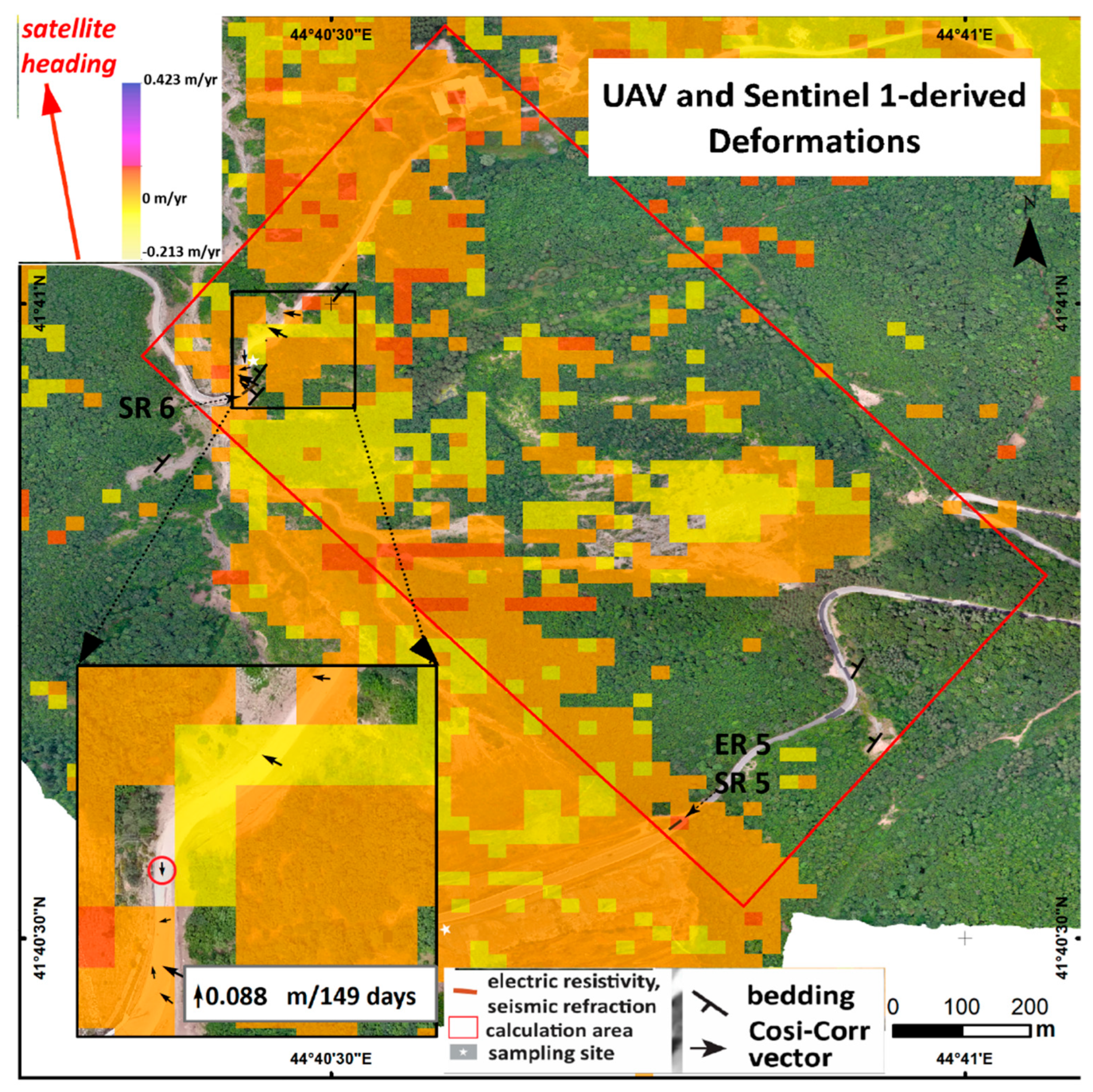
Within the investigated slope defined by calculation area in Figure 8, 687 valid 20 × 20 m pixels were retained, corresponding to an analyzed area of approximately 0.275 km². LOS velocities range from -15.7 to +38.3 mm yr-¹, with a mean of +9.2 mm yr⁻¹ and a median of +9.5 mm yr-¹. The robust 5th–95th percentile interval is -8.0 to +25.3 mm yr-¹, demonstrating that the observed deformation pattern is not controlled by a small number of extreme pixels. Positive LOS velocities occur in 561 of the 687 pixels (81.7%), indicating that motion toward the satellite dominates the investigated slope. Pixel-wise velocity uncertainty is comparatively low, with mean and median velocity standard deviations of 1.47 and 1.46 mm yr-¹, respectively. The displacement time series comprises 109 Sentinel 1 acquisitions between 2 April 2022 and 31 October 2025 and is referenced to 24 August 2022. The spatial-median LOS displacement reaches +50.3 mm at the final acquisition relative to the reference date, while the net median displacement change between the first and final acquisitions is approximately +37.9 mm. Despite short-term temporal fluctuations, the time series therefore supports the persistent positive LOS deformation indicated by the velocity field.
The analysis in COSI-Corr showed mean apparent offsets of -0.85 mm in the E-W component and -13.92 mm in the N-S component, with corresponding standard deviations of 8.44 and 10.12 mm. After removal of these mean biases, the 95th percentile of the stable-ground horizontal residuals was 0.0235 m, which was adopted as the empirical relative displacement detection threshold (MDD₉₅). Re-filtering the COSI-Corr results using the SNR and displacement criteria yielded a final set of seven spatially coherent vectors. Their horizontal displacement magnitudes ranged from 0.0495 to 0.0880 m, with a mean of 0.0658 m and a median of 0.0643 m. SNR values ranged from 0.9901 to 0.9939. The retained COSI-Corr vectors ranged from 0.0495 to 0.0880 m and exceeded the empirical stable-ground detection threshold by approximately 2.1 - 3.8 times. This supports their interpretation as plausible slope-related displacement rather than typical residual co-registration noise. However, because the measured deformation remains centimetre-scale and only two independent checkpoints were available for each epoch, higher-order photogrammetric distortion cannot be completely excluded. The UAV/COSI-Corr results are therefore interpreted as complementary evidence of slow slope deformation rather than as an independently definitive displacement field (Figure 8).
Kinematic consistency check showed that, the mean COSI-Corr displacement azimuth was approximately 2820, while the ascending Sentinel-1 ground to satellite look azimuth was approximately 2570. The angular difference was therefore 250, giving a horizontal directional projection coefficient of cos (250) =0.906. This positive coefficient indicates that the UAV-derived horizontal displacement is oriented toward the Sentinel-1 sensor, consistent in sign with the positive LOS deformation observed by InSAR. Should be noted that, because the UAV measurements do not constrain vertical displacement, this agreement is interpreted as a kinematic consistency check rather than a quantitative reconstruction of the complete LOS displacement.
If we look in complex all these data, Figure 9 shows a consistent westerly to north-northwesterly orientation across all three datasets, with bedding dip direction, slope aspect, and COSI-Corr displacement azimuth converging on a broadly common downslope sector. Nevertheless, the three distributions are slightly offset, with displacement oriented marginally counter-clockwise relative to both the topographic and structural directions.
4.2. Rainfall Extreme-Value Analysis Results
The largest daily precipitation value in the 41-year annual-maxima series was 123.8 mm, recorded in 1979. Maximum-likelihood fitting of the Gumbel distribution produced a location parameter of 37.19 mm and a scale parameter of 18.49 mm. The Anderson-Darling statistic was 0.661, with a Monte Carlo p-value was 0.086; therefore, the Gumbel distribution was not rejected at the 5% significance level.
The GEV model produced a slightly lower AICc than the Gumbel model (376.83 and 377.35, respectively), but the difference was small (ΔAICc=0.52). Similarly, the likelihood-ratio test did not indicate a statistically significant improvement from introducing the additional GEV shape parameter (p=0.091). Even though, the model-selection uncertainty increases for long return periods, the two-parameter Gumbel distribution was retained as the more careful model. Uncertainty increases significantly with increasing return period, as expected given the limited length of the observational record (Table 3). Accordingly, the 500- and particularly the 1000-year estimates should be interpreted as indicative extreme-event ranges rather than precisely constrained recurrence levels.
4.3. Sensitivity of Slope Response to Pore-Pressure Ratio
The LS-RAPID sensitivity analysis showed a dependence of the simulated slope response on the prescribed pore-pressure ratio (ru). For ru =0.05, no non-zero U or V values were recorded during the 7200 s simulation, indicating that no modelled movement developed within the analysed time interval. At ru =0.15, the first recorded non-zero velocity occurred at 675 s. Increasing ru to 0.20, 0.25, and 0.30 progressively reduced this time to 525, 515, and 490 s, respectively. The largest reduction within this intermediate range occurred between ru =0.15 and 0.20, for which an increase of 0.05 in ru reduced the time to first recorded movement by 150 s (22.2%).
A substantially different response was obtained at higher pore-pressure ratios. For both ru =0.40 and 0.45, the first non-zero velocity was recorded at 95 s, representing an approximately 81% reduction relative to the ru =0.30 case. Significantly different response was obtained at higher pore-pressure ratios. For both ru=0.40 and 0.45, the first recorded non-zero velocity occurred at 95 s, representing an approximately 81% reduction relative to the ru=0.30 scenario. Overall, the simulations show a nonlinear decrease in movement-onset time with increasing prescribed ru, with a marked transition from delayed movement at ru=0.15 - 0.30 to rapid movement at ru=0.40 - 0.45. Overall, the resulted simulations show a nonlinear decrease in the time to recorded movement with increasing ru, with a marked transition from delayed movement at ru =0.15-0.30 to rapid movement at ru =0.40.
The ru sensitivity analysis in the Figure 10 showed a nonlinear response to increasing ru. No recorded movement occurred for ru =0.05 during the extended 7200 s simulation. A markedly faster response occurred at ru =0.40 and 0.45, for which movement was first recorded at 95 s. These results indicate three broad behavioural regimes: no recorded movement under the tested low ru condition, delayed movement for ru =0.15 and 0.30 and rapid movement for ru =0.40 and 0.45. The simulations are interpreted as sensitivity scenarios rather than as determination of exact critical ru thresholds. Accordingly, the purpose of the sensitivity analysis was not to determine a precise critical ru value, but to identify broad changes in model behaviour under progressively higher prescribed pore-pressure conditions. Therefore, no attempt was made to interpolate between the tested scenarios or to define exact transition thresholds where the available input data did not support such precision (simulation files are presented in Supplementary Material 2).
5. Discussions and Conclusions
The combined observations indicate that the slope adjacent to the 2015 landslide source area cannot be regarded as completely inactive. The small-baseline InSAR analysis identifies spatially coherent positive LOS deformation within and around the previous landslide area, including parts of the adjacent forested slope. The area also indicates signs of instability into the results of the UAV-based analysis. After correction for systematic offsets and application of the empirical detection threshold, the retained COSI-Corr vectors show displacements of approximately 0.05-0.09 m over 149 days. These values exceed the stable-ground detection threshold by more than a factor of two and therefore are substantially larger than the typical stable-ground residuals and tend to support their interpretation as plausible slope-related displacement. But as the magnitude of the displacement remains small, the results should be interpreted as evidence of slow ongoing deformation rather than an indication of imminent large-scale failure.
The directional relationship between the observed displacement, slope morphology, and geological structure provides additional support for this interpretation. The mean bedding dip direction of ~3440, mean slope aspect of ~3200 and mean COSI-Corr displacement azimuth of ~2820 all fall within a broadly westerly to north-northwesterly sector. This general agreement suggests that the measured surface movement is consistent with the downslope geometry and with the structural configuration of the layered bedrock. The Cosi-Corr displacement direction is nevertheless a bit off from both the mean slope aspect and bedding dip direction. This can be indicating that movement is unlikely to be controlled by a single planar factor. This deviation may reflect the combined influence of heterogeneous weathering, local slope morphology and the orientation of fractures, joints, and faults within the rock mass.
The ru simulations were intended to identify broad behavioural ranges rather than precise hydrological thresholds. The absence of intermediate simulations between ru =0.05 and 0.15 and between ru =0.30 and 0.40 reflects the uncertainty of the available subsurface and material data. Densely sampling these intervals could imply a degree of precision that is not supported by the data constraints. Accordingly, the results are interpreted as scenario bracketing - a low ru condition with no recorded movement, an intermediate range characterized by delayed movement and a higher ru range characterized by rapid model response.
The rainfall analysis and its fitted extreme-value distribution gave precipitation estimates of 152.1 mm and 164.9 mm for the 500- and 1000-year return periods. However, the rainfall return-period estimates provide here just the hydrometeorological context, whereas the LS-RAPID simulations explore how the slope responds to prescribed pore-pressure conditions.
Several limitations should be acknowledged. The ascending-only InSAR data provide LOS rather than full three-dimensional displacement and are less reliable over dense vegetation, while the centimetre-scale UAV/COSI-Corr results remain sensitive to residual co-registration and image-correlation errors despite the use of an empirical detection threshold and independent checkpoints. Numerical uncertainty is also present because the 4 m rupture depth simplifies the true complex subsurface geometry. Also the effective shear resistance includes an assumed root-reinforcement contribution and the prescribed ru values represent sensitivity scenarios rather than measured pore pressures. Accordingly, LS-RAPID is used here to explore the slope’s sensitivity to pore-pressure changes rather than to predict an exact future failure time.
The combined observations are consistent with slow ongoing slope deformation and remains sensitive to hydrological changes. The spatial and directional agreement between the InSAR and UAV observations and the geological and topographic setting strengthens the interpretation that the measured displacement represents slope-related movement. Additionally, the modelling shows that relatively modest changes in pore-pressure conditions can lead to a strongly nonlinear change in slope response. Should be noted that these findings do not demonstrate that a new major failure is imminent, but they indicate that the area should not be considered permanently stabilized following the 2015 event.
This conclusion is important in the Vere valley, where the consequences of slope instability extend beyond the source area itself. The 2015 disaster demonstrated how a hillslope failure can translate into the cascading event causing casualties and damaging urban infrastructure into the densely populated city. Continued development within the downstream corridor therefore makes the identifying of slowly deforming slopes relevant to broader risk management. Periodic InSAR screening combined with targeted UAV surveys, field observations and, where possible, direct groundwater and pore-pressure monitoring would provide a practical basis for determining whether the deformation identified in this study remains approximately steady or begins to accelerate.
Supplementary Materials
The following supporting information can be downloaded at the website of this paper posted on Preprints.org.
Author Contributions
Lasha Sukhishvili: conceptualization, Small-Baseline InSAR Time-Series Analyses, UAV photogrammetry and COSI_Corr analysis, rainfall analysis, landslide numerical simulation, and manuscript writing. Salome Gogoladze: geological sampling, laboratory analyses, and manuscript editing. Giorgi Merebashvili: landslide numerical simulation. Givi Gventsadze and Linda Nakashidze: GNSS data collection and processing.
Funding
This work was supported by Shota Rustaveli National Science Foundation of Georgia (SRNSFG), grant number: YS-22-826.
Data Availability Statement
The raw data supporting the conclusions of this article will be made available by the authors on request.
Conflicts of Interest
The authors declare no conflicts of interest.
References
- Iverson, R. M. Landslide triggering by rain infiltration. Water Resour. Res. 2000, vol. 36(no. 7), 1897–1910. [Google Scholar] [CrossRef]
- Guzzetti, F.; Peruccacci, S.; Rossi, M.; Stark, C. P. Rainfall thresholds for the initiation of landslides in central and southern Europe. Meteorol. Atmos. Phys. 2007, vol. 98(no. 3–4), 239–267. [Google Scholar] [CrossRef]
- Petley, D. N.; Bulmer, M. H.; Murphy, W. Patterns of movement in rotational and translational landslides. Geology 2002, vol. 30(no. 8), 719–722. [Google Scholar] [CrossRef]
- Berardino, P.; Fornaro, G.; Lanari, R.; Sansosti, E. A new algorithm for monitoring localized deformation phenomena based on small baseline differential SAR interferograms. Int. Geosci. Remote Sens. Symp. 2002, vol. 2(no. 11), 1237–1239. [Google Scholar] [CrossRef]
- Casagli, N.; Intrieri, E.; Tofani, V.; Gigli, G.; Raspini, F. Landslide detection, monitoring and prediction with remote-sensing techniques. Nat. Rev. Earth Environ. 2023, vol. 4(no. 1), 51–64. [Google Scholar] [CrossRef]
- Schlögl, M.; Gutjahr, K.; Fuchs, S. The challenge to use multi-temporal InSAR for landslide early warning. Nat. Hazards 2022, vol. 112(no. 3), 2913–2919. [Google Scholar] [CrossRef]
- James, M. R.; Robson, S. “Mitigating systematic error in topographic models derived from UAV and ground-based image networks,”. Earth Surf. Process. Landf. 2014, vol. 39(no. 10), 1413–1420. [Google Scholar] [CrossRef]
- James, M. R.; Robson, S.; d’Oleire-Oltmanns, S.; Niethammer, U. Optimising UAV topographic surveys processed with structure-from-motion: Ground control quality, quantity and bundle adjustment. Geomorphology 2017, vol. 280, 51–66. [Google Scholar] [CrossRef]
- K. Ajmera, B.; Emami Ahari, H.; Loi, D.H.; Setiawan, H.; Dang, K.; Sassa. LS-RAPID Man. With Video Tutor. 2023, vol. Part F4144(no. 1). [CrossRef]
- Institute of Earth Sciences and National Seismic Monitoring Center. Multidisciplinary Investigation of Akhaldaba Landslide (in Georgian); Tbilisi, 2015. [Google Scholar]
- Kereselidze, D.; Alaverdashvili, M.; Tsintsadze, T.; Trapaidze, V.; Bregvadze, G. What happened on June 13, 2015, in the Vere River gorge in Tbilisi (in Georgian); Tbilisi, 2015. [Google Scholar]
- Bennett, K.; Gosselin-campbell, J.; Schnackenberg, L. Tbilisis Flood 2015 - Initial Findings and Response Actions. 2015. [Google Scholar]
- Gregory, K. J.; Wallingford, D. E. DRAINAGE BASIN FORM AND PROCESS - A GEOMORPHOLOGICAL APPROACH. 1973, no. [Google Scholar]
- Schumm, S. A. Geological Society of America Bulletin EVOLUTION OF DRAINAGE SYSTEMS AND SLOPES IN BADLANDS AT PERTH AMBOY, NEW JERSEY. Bull. Geol. Soc. Am. vol. 67(no. 5), 597–646, 1956.
- Gaprindashvili, G.; Gaprindashvili, M.; Tsereteli, E. Natural Disaster in Tbilisi City ( Riv. Vere Basin ) in the Year 2015. 2016, vol. 2016, 1074–1087. [Google Scholar] [CrossRef]
- Mesa, L. M. Morphometric analysis of a subtropical Andean basin (Tucumán, Argentina). Environ. Geol. 2006, vol. 50(no. 8), 1235–1242. [Google Scholar] [CrossRef]
- Torres, R.; et al. GMES Sentinel-1 mission. Remote Sens. Environ. 2012, vol. 120, 9–24. [Google Scholar] [CrossRef]
- Lanari, R.; Mora, O.; Manunta, M.; Mallorquí, J. J.; Berardino, P.; Sansosti, E. A small-baseline approach for investigating deformations on full-resolution differential SAR interferograms. IEEE Trans. Geosci. Remote Sens. 2004, vol. 42(no. 7), 1377–1386. [Google Scholar] [CrossRef]
- Hooper; Bekaert, D.; Spaans, K.; Arikan, M. Recent advances in SAR interferometry time series analysis for measuring crustal deformation. Tectonophysics 2012, vol. 514–517, 1–13. [Google Scholar] [CrossRef]
- Yunjun, Z.; Fattahi, H.; Amelung, F. Small baseline InSAR time series analysis: Unwrapping error correction and noise reduction. Comput. Geosci. 2019, vol. 133, 104331. [Google Scholar] [CrossRef]
- Jolivet, R.; Grandin, R.; Lasserre, C.; Doin, M. P.; Peltzer, G. Systematic InSAR tropospheric phase delay corrections from global meteorological reanalysis data. Geophys. Res. Lett. 2011, vol. 38(no. 17), 1–6. [Google Scholar] [CrossRef]
- Fattahi, H.; Amelung, F. DEM error correction in InSAR time series. IEEE Trans. Geosci. Remote Sens. 2013, vol. 51(no. 7), 4249–4259. [Google Scholar] [CrossRef]
- Hastaoğlu, K. Ö.; Gül, Y.; Poyraz, F.; Kara, B. C. Monitoring 3D areal displacements by a new methodology and software using UAV photogrammetry. Int. J. Appl. Earth Obs. Geoinf. 2019, vol. 83, no. June, 101916. [Google Scholar] [CrossRef]
- Eker, R.; Aydın, A. Long-term retrospective investigation of a large, deep-seated, and slow-moving landslide using InSAR time series, historical aerial photographs, and UAV data: The case of Devrek landslide (NW Turkey). CATENA 2021, vol. 196, 104895. [Google Scholar] [CrossRef]
- Forlani, G.; Dall’Asta, E.; Diotri, F.; di Cella, U. M.; Roncella, R.; Santise, M. Quality assessment of DSMs produced from UAV flights georeferenced with on-board RTK positioning. Remote Sens. 2018, vol. 10(no. 2). [Google Scholar] [CrossRef]
- Štroner, M.; Urban, R.; Reindl, T.; Seidl, J.; Brouček, J. Evaluation of the georeferencing accuracy of a photogrammetric model using a quadrocopter with onboard GNSS RTK. Sensors 2020, vol. 20(no. 8). [Google Scholar] [CrossRef]
- Stott, E.; Williams, R. D.; Hoey, T. B. Ground control point distribution for accurate kilometre-scale topographic mapping using an rtk-gnss unmanned aerial vehicle and sfm photogrammetry. Drones 2020, vol. 4(no. 3), 1–21. [Google Scholar] [CrossRef]
- Štroner, M.; Urban, R.; Seidl, J.; Reindl, T.; Brouček, J. Photogrammetry using UAV-mounted GNSS RTK: Georeferencing strategies without GCPs. Remote Sens. 2021, vol. 13(no. 7). [Google Scholar] [CrossRef]
- Tavasci, L.; Nex, F.; Gandolfi, S. Reliability of Real-Time Kinematic (RTK) Positioning for Low-Cost Drones’ Navigation across Global Navigation Satellite System (GNSS) Critical Environments. Sensors 2024, vol. 24(no. 18). [Google Scholar] [CrossRef]
- Leprince, S.; Barbot, S.; Ayoub, F.; Avouac, J.-P. Automatic and Precise Orthorectification, Coregistration, and Subpixel Correlation of Satellite Images, Application to Ground Deformation Measurements. IEEE Trans. Geosci. Remote Sens. 2007, vol. 45(no. 6), 1529–1558. [Google Scholar] [CrossRef]
- Ayoub, F.; Leprince, S.; Avouac, J.-P. Co-registration and correlation of aerial photographs for ground deformation measurements. ISPRS J. Photogramm. Remote Sens. 2009, vol. 64(no. 6), 551–560. [Google Scholar] [CrossRef]
- Wu, T. H.; McKinnell, W. P.; Swanston, D. N. Strength of Tree Roots and Landslides on Price of Wales Island, Alaska. Can. Geotech. J. 1979, vol. 16(no. 1), 19–33. [Google Scholar] [CrossRef]
- Schwarz, M.; Cohen, D.; Or, D. Root-soil mechanical interactions during pullout and failure of root bundles. J. Geophys. Res. Earth Surf. 2010, vol. 115(no. 4), 1–19. [Google Scholar] [CrossRef]
- Cohen, D.; Schwarz, M. Tree-root control of shallow landslides. Earth Surf. Dyn. 2017, vol. 5(no. 3), 451–477. [Google Scholar] [CrossRef]
Figure 1.
Location and drainage network of the Vere River basin, Tbilisi, Georgia.
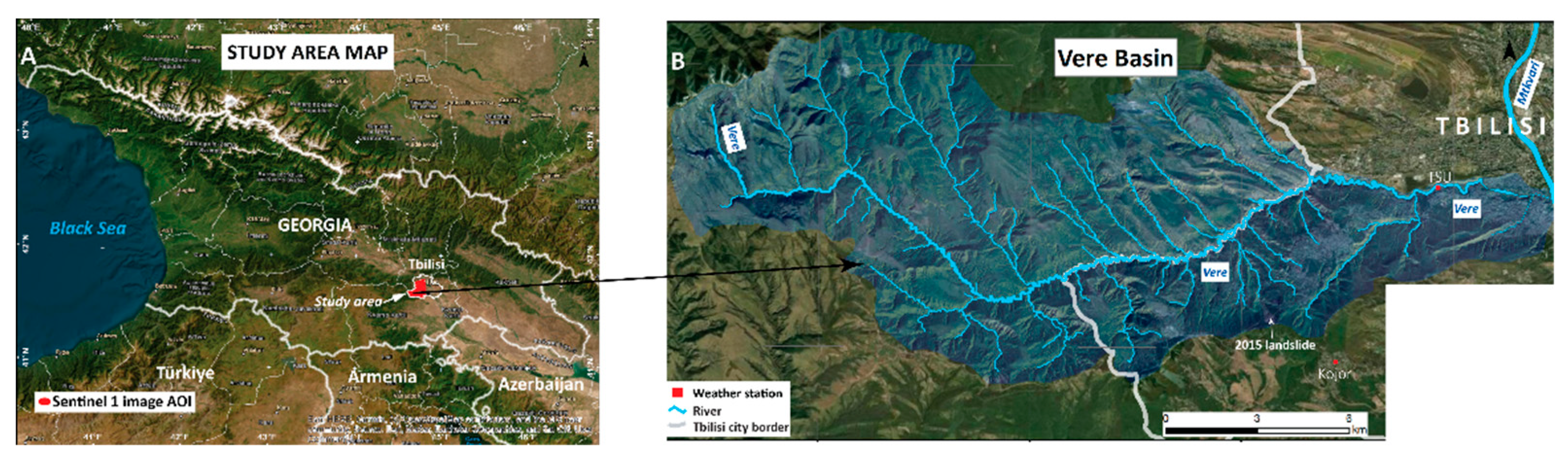
Figure 2.
The image was taken in June 2015 in the source zone of the major landslide.
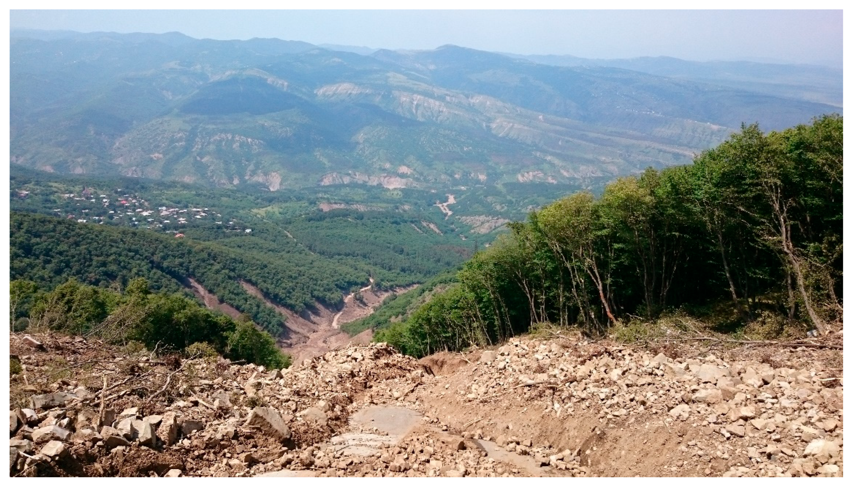
Figure 3.
Field evidence of fractured and weathered layered bedrock in the landslide source area.
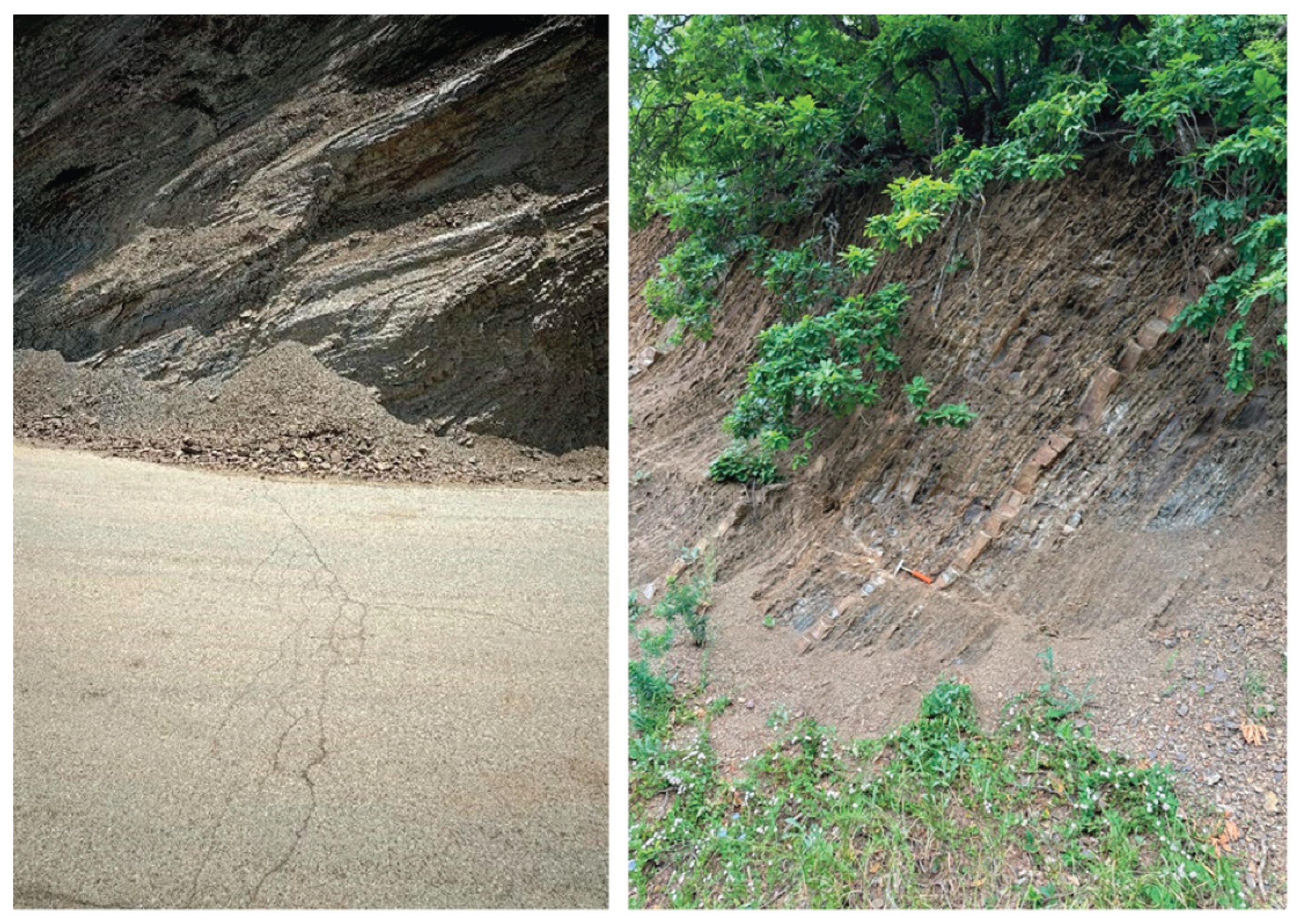
Figure 4.
The climate diagrams for the TSU Hydrometeorological Lab (460 m) and Kojori (1340 m) stations. The blue bars represent monthly precipitation (mm), and the red lines represent average monthly temperature (°C). The data represents 1963-2015 observation years and is taken from [11]).
Figure 4.
The climate diagrams for the TSU Hydrometeorological Lab (460 m) and Kojori (1340 m) stations. The blue bars represent monthly precipitation (mm), and the red lines represent average monthly temperature (°C). The data represents 1963-2015 observation years and is taken from [11]).
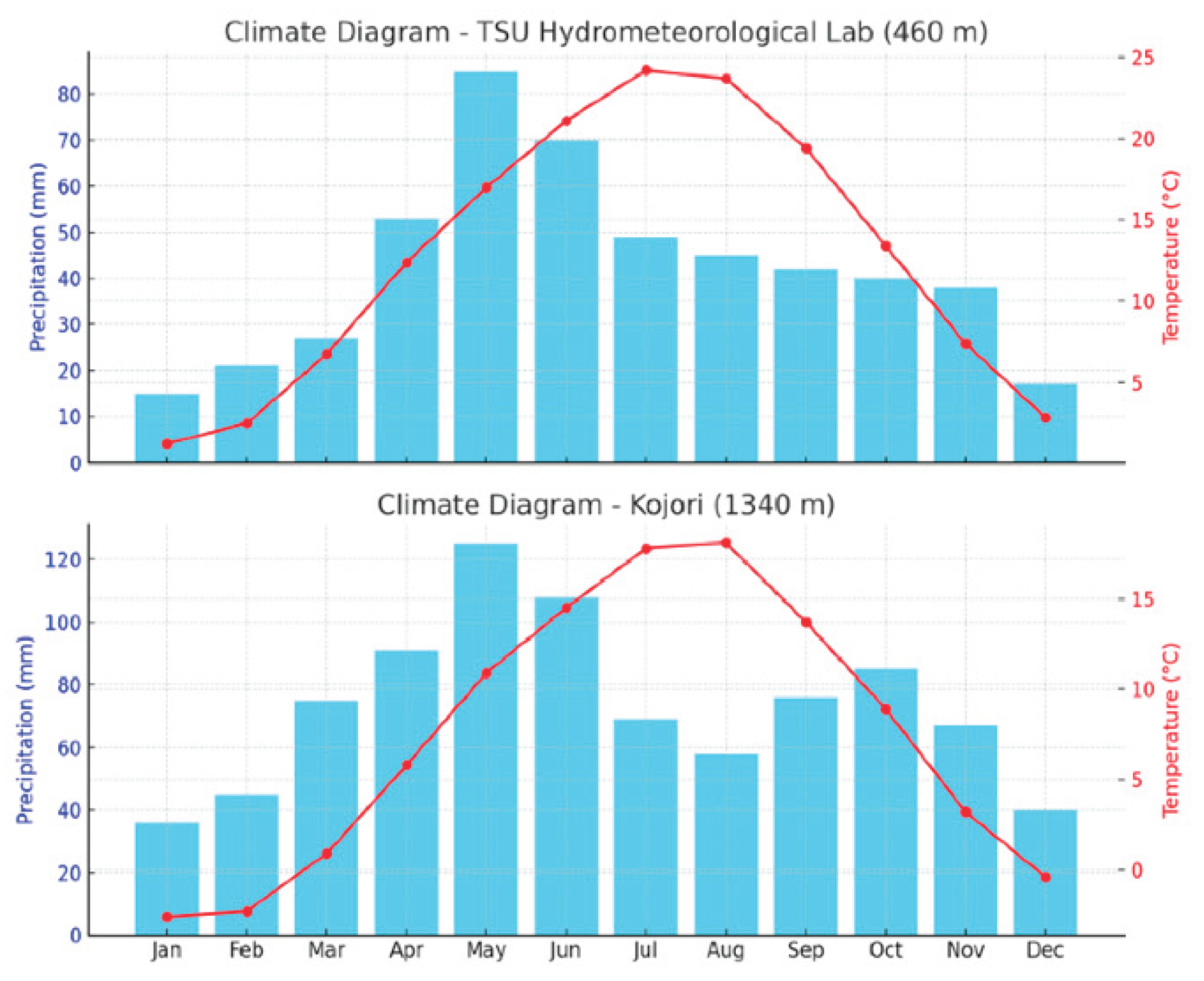
Figure 5.
UAV-derived orthomosaics used for multi-temporal slope deformation analysis. A. shows the full orthomosaic of the study area acquired on 28 June 2024, covering approximately 1.9 × 1.9 km. The lower panels show the smaller targeted area selected for multi-temporal comparison. B. Orthomosaics from 7 October 2024; and C. 5 March 2025 were used for image co-registration and horizontal displacement analysis. The black arrows indicate the location of the detailed monitoring area within the wider UAV survey.
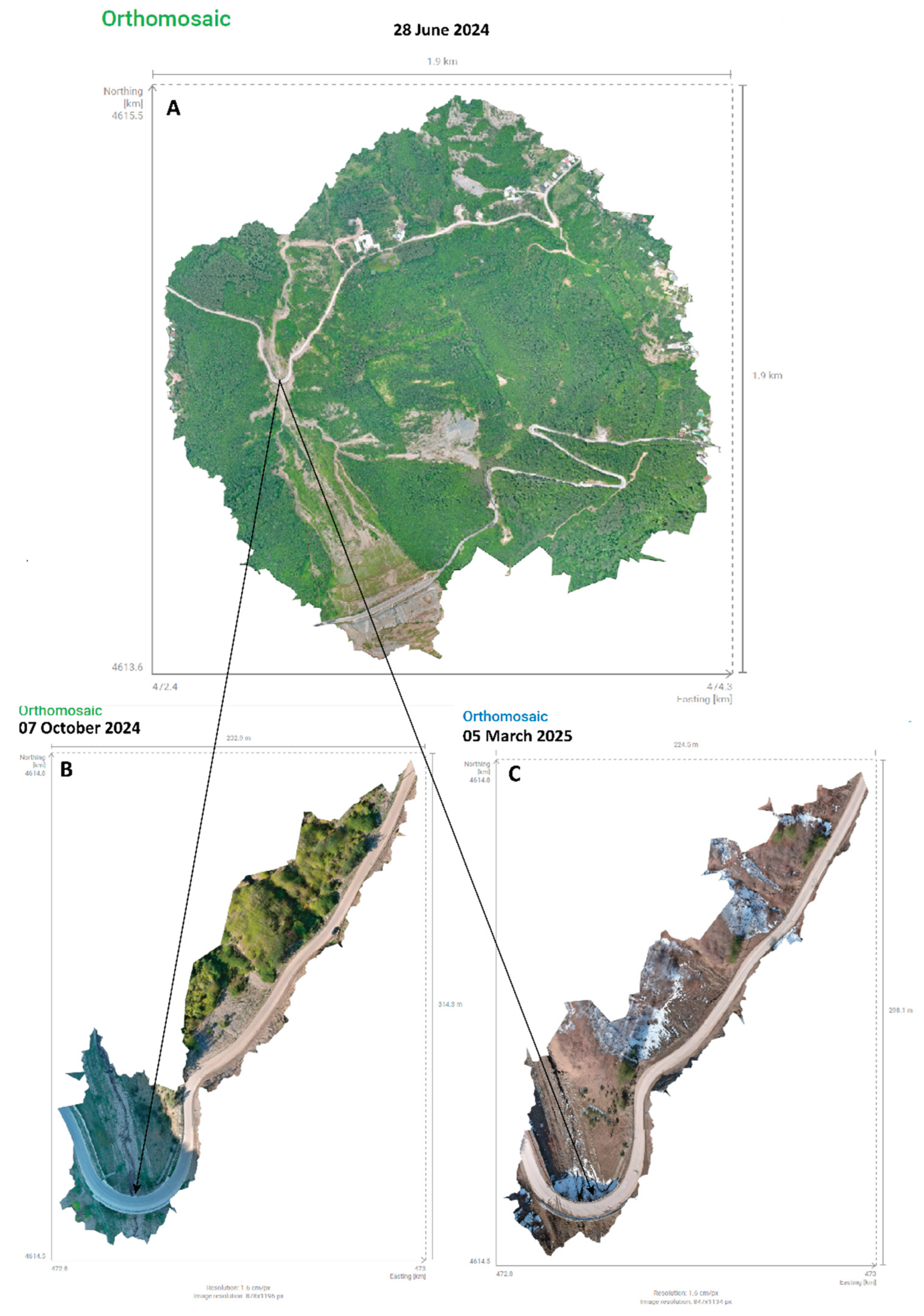
Figure 6.
Geophysical constraints on the inferred rupture surface in the landslide source area.
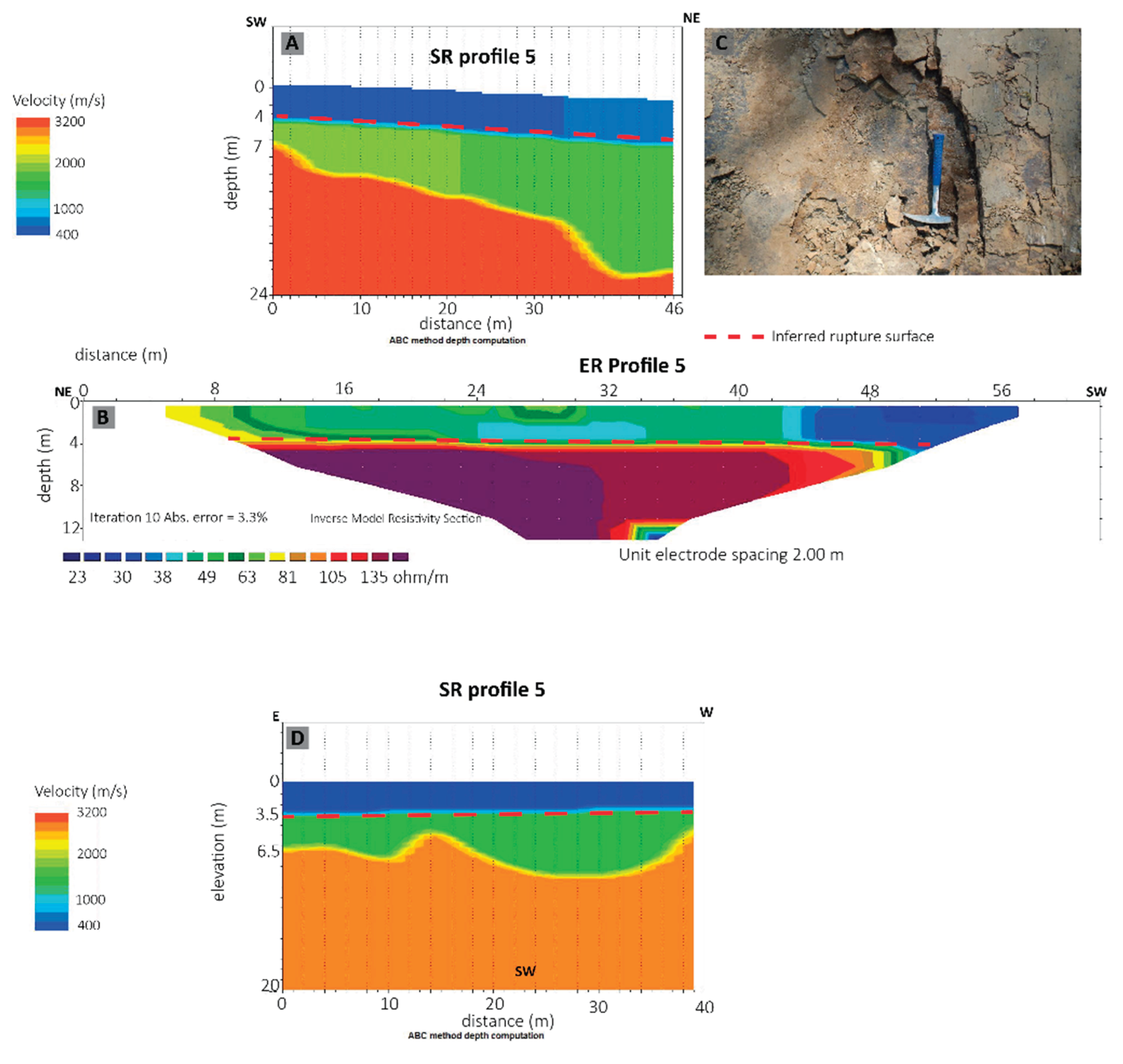
Figure 7.
Representative SBAS InSAR LOS displacement time series for the investigated slope, calculated from the 687 valid pixels within the calculation area shown on the Figure 8. The solid line shows the spatial median displacement for each Sentinel 1 acquisition, the darker shaded band represents the interquartile range (25th-75th percentiles), and the lighter shaded band indicates the 5th-95th percentile range. Displacements are referenced to 24 August 2022; positive values indicate motion toward the satellite.
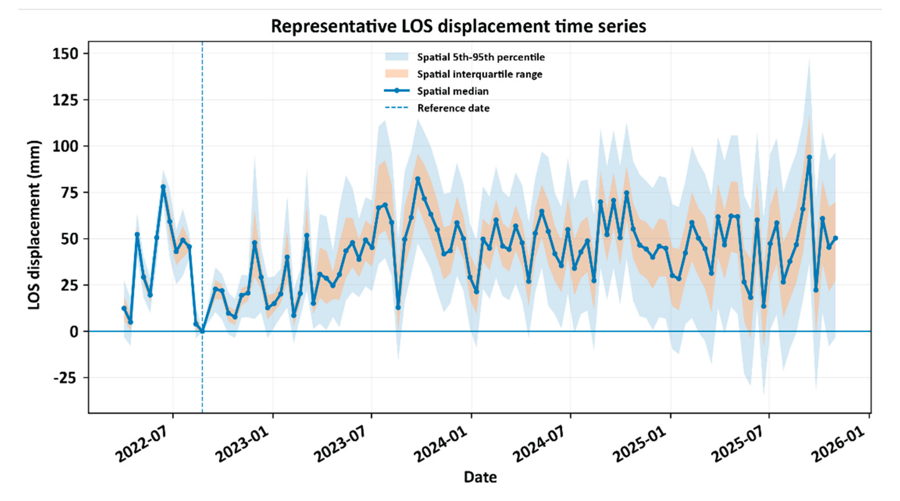
Figure 9.
Directional comparison of structural, topographic, and kinematic azimuths. Wedges show the central 50% of each distribution; arrows indicate circular means. Bedding dips toward 344°, slope aspect toward 320°, and UAV-derived COSI-Corr displacement toward 282°. Azimuths increase clockwise from north; radial position is arbitrary and separates the three datasets.
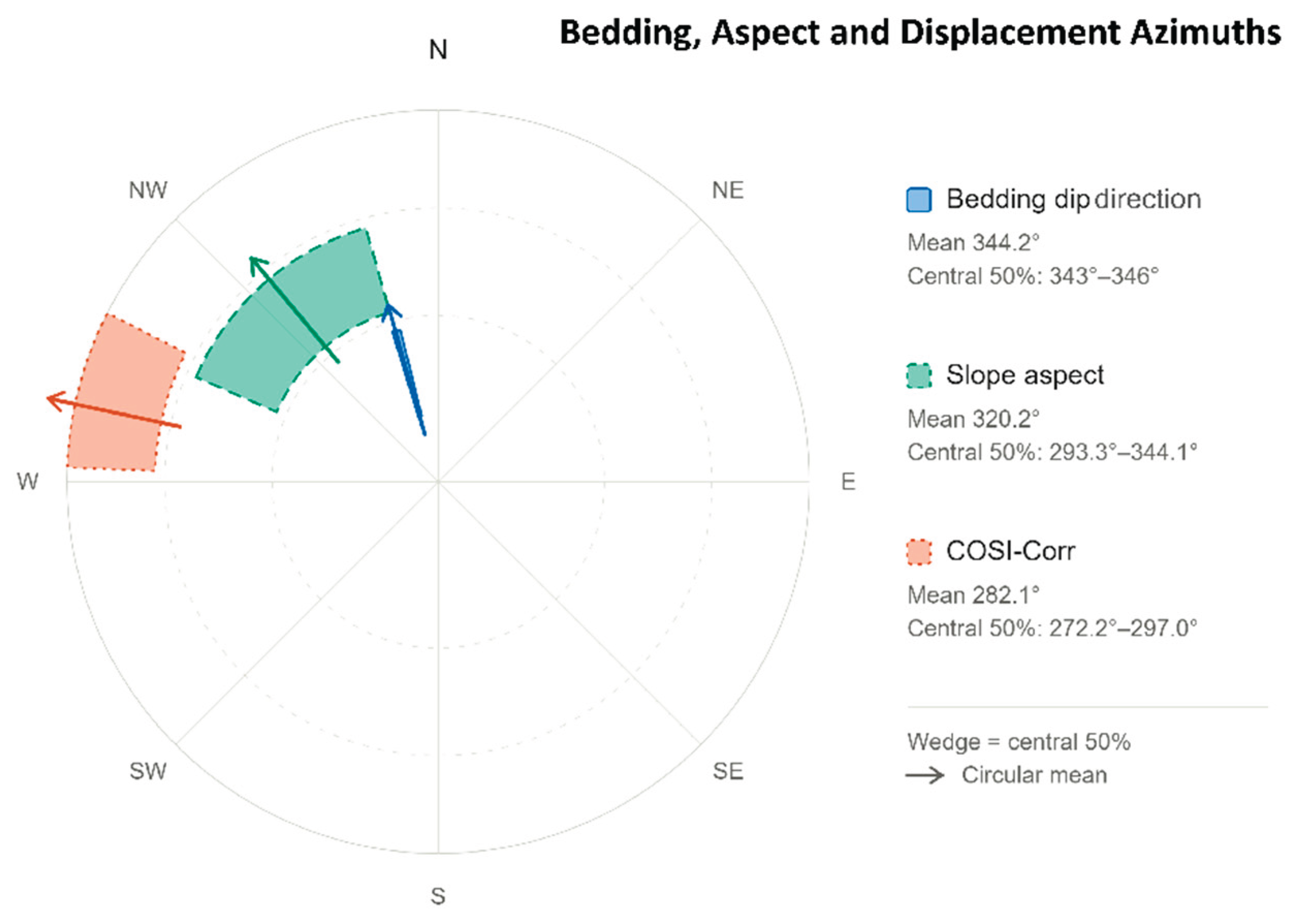
Figure 10.
Sensitivity of the simulated slope response to prescribed pore-pressure ratio (), expressed as the time to first recorded movement.
Figure 10.
Sensitivity of the simulated slope response to prescribed pore-pressure ratio (), expressed as the time to first recorded movement.
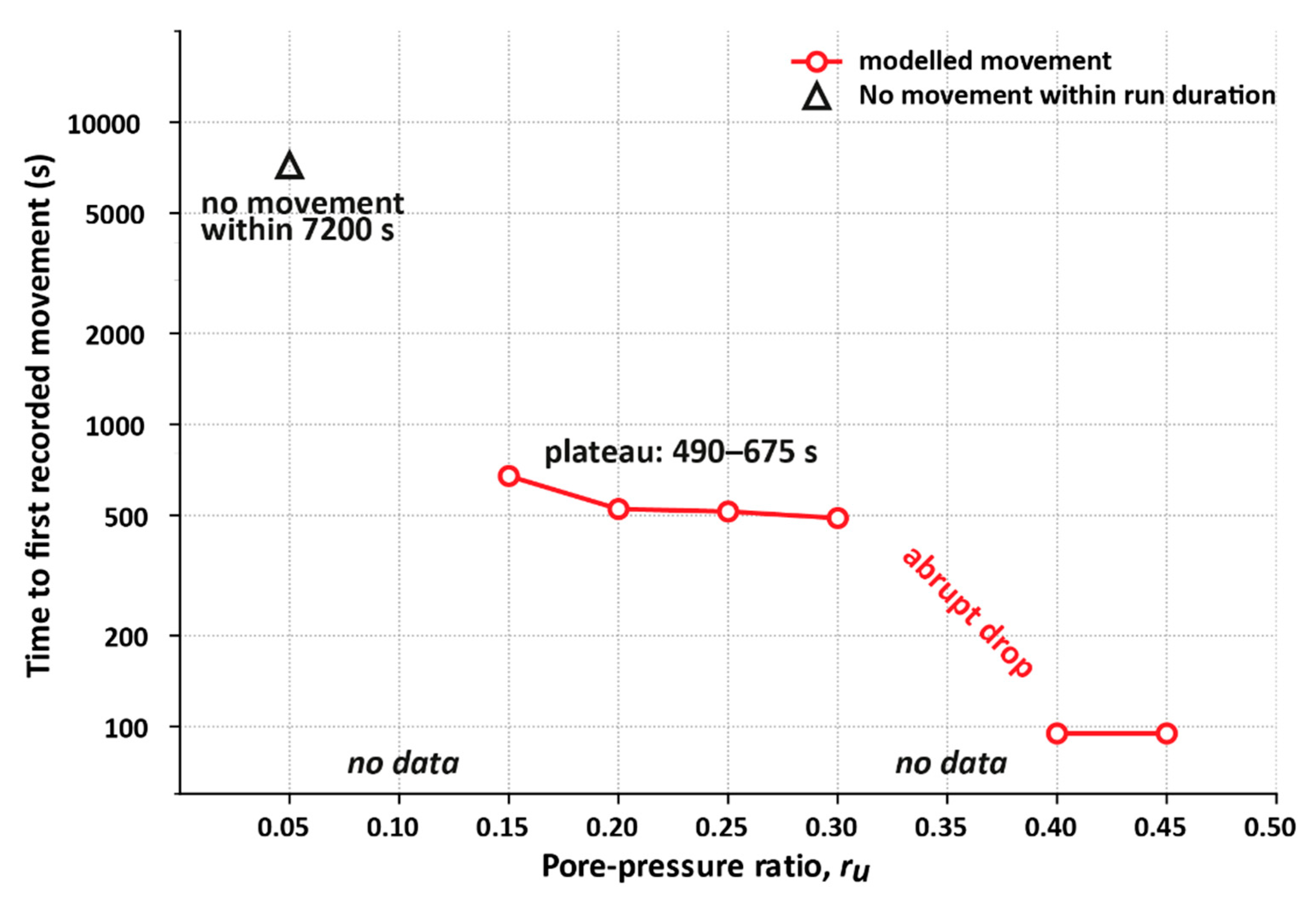

Table 1.
Summary of me the TSU Hydrometeorological Lab and Kojori meteorological stations.
| Parameter | TSU Lab (460 m) | Kojori (1340 m) |
| Annual Mean Temp (°C) | ~12.9°C | ~8.5°C |
| Hottest Month | July (24.2°C) | August (18.1°C) |
| Coldest Month | January (1.2°C) | January (–2.6°C) |
| Thermal Amplitude Mean Annual Precipitation |
~23°C 502mm |
~21°C 875mm |
Table 2.
Geophysical and laboratory-derived parameters used to constrain the LS-RAPID slope stability simulation.
Table 2.
Geophysical and laboratory-derived parameters used to constrain the LS-RAPID slope stability simulation.
| Parameter | Value | Source |
| Rupture surface depth | 4 m | ER and SR [10] |
| Unit weight of mass (γ) | 21.48 kN/m3 | [10] |
| Porosity | 22.99% | [10] |
| Rate of excess pore-pressure generation | 0 (no additional shear-induced excess pore-pressure generation) | |
| Pore-pressure ratio ru | 0.05 - 0.45 | prescribed separately for each sensitivity scenario |
| Steady state shear resistance at sliding surface | 1 kPa laboratory baseline; 5 kPa effective calibrated model value | Laboratory analyses |
| Friction angle (φ) | 340 | Laboratory analyses |
Table 3.
The results of the Gumbel return levels and their 95% bootstrap confidence intervals.
| Return period (years) | Return level (mm) | 95% confidence interval (mm) |
| 100 | 122 | 99.1 – 144.9 |
| 500 | 152 | 121.7-181.5 |
| 1000 | 165 | 131.4 - 197.4 |
Disclaimer/Publisher’s Note: The statements, opinions and data contained in all publications are solely those of the individual author(s) and contributor(s) and not of MDPI and/or the editor(s). MDPI and/or the editor(s) disclaim responsibility for any injury to people or property resulting from any ideas, methods, instructions or products referred to in the content. |
© 2026 by the authors. Licensee MDPI, Basel, Switzerland. This article is an open access article distributed under the terms and conditions of the Creative Commons Attribution (CC BY) license (http://creativecommons.org/licenses/by/4.0/).
Copyright: This open access article is published under a Creative Commons CC BY 4.0 license, which permit the free download, distribution, and reuse, provided that the author and preprint are cited in any reuse.