

Submitted:
02 October 2026
Posted:
05 October 2026
You are already at the latest version
Abstract
This study establishes a harmonized worldwide statistical atlas of principal-landmass national border complexity, addressing the absence of any dataset estimating their fractal dimensions under one common dual-method framework. Box-counting and divider fractal dimensions were estimated for 197 countries and territories from consistently processed GADM 4.1 geometries and evaluated at continental and global levels. Most principal-landmass borders proved measurably fractal yet occupied a comparatively low complexity band, departing from the linear benchmark while remaining far from plane-filling geometry: the worldwide mean dimensions were 1.0959 and 1.0975, respectively, with no evidence of a systematic paired difference (mean difference = −0.0015). Cross-method correspondence was strong (Pearson r = 0.9155; Lin CCC = 0.9069), although Bland–Altman and rank analyses identified modest magnitude-dependent disagreement and a limited set of method-sensitive countries. The equal-weight consensus fractal dimension averaged 1.0967 worldwide, ranging from 1.0170 for Somalia to 1.3615 for Norway, and continental consensus averages were highest in North America (1.1259) and Europe (1.1150) and lowest in Africa (1.0652). With all source geometries, candidate scales, and estimates archived for replication, the country-level values form a reproducible baseline for comparative, sensitivity, and time-indexed analyses of national-border complexity.
Keywords:
border
; fractal dimension
; method agreement
; spatial statistics
1. Introduction
1.1. Fractal Geometry of Geographical Boundaries
Geographical boundaries are scale-dependent curves whose measured complexity can change with the spatial resolution at which they are examined. Richardson showed that the measured length of an irregular geographical curve depends systematically on the measuring unit, and Mandelbrot later placed this behavior within the framework of fractal geometry [1,2]. For a planar boundary, a fractal dimension near corresponds to comparatively line-like geometry, whereas larger values toward indicate increasing irregularity and spatial occupancy. Divider and box-counting procedures provide two established but geometrically distinct ways of estimating this scaling behavior, and their finite-scale results need not be identical for the same boundary [3].
1.2. From Boundary Fractality to a World Atlas
Fractal analysis has been applied extensively to natural shorelines, coastlines, islands, and related geographical curves, from the classical coastline problem to recent large-scale analyses of Earth’s islands [2,4,5,6,7]. Political boundaries have received comparatively less systematic treatment. Longley and Batty provided an early geographical framework for fractal boundary measurement, and Alesina et al. later incorporated border fractality into a broad cross-national analysis of political states [3,8]. However, the available literature has not produced a harmonized worldwide dataset in which the principal national landmass boundaries are defined consistently and estimated by both box-counting and divider methods under one common computational framework.
The present study serves as the final step in a progressive sequence of paired adaptive country specific analyses [9,10]. The first step was taken in the Iran study in which it applied box-counting and divider estimation at the national level and within a 13 companion West Asian regional comparisons, establishing a reproducible dual-method framework for political boundaries [9]. The subsequent step was taken in the Canada study in which it extended this hierarchy from the national level to North America and then to a standardized comparison of 31 major principal landmasses worldwide [10]. Together, these studies provided the methodological basis for moving from country-centred comparisons to a genuinely worldwide analysis.
1.3. Study Objective
The present World Statistical Atlas completes that progression by applying a common geospatial, adaptive-scale, and dual-method procedure to the principal connected landmass boundaries of 197 countries and territories (Figure 1). Its objectives are to estimate country-level box-counting and divider fractal dimensions, summarize their continental and worldwide distributions, quantify cross-method agreement and rank stability, identify method-sensitive countries, and provide an equal-weight consensus dimension as a compact descriptive reference. By placing all study units within the same analytical system, the Atlas is intended to provide an internally standardized worldwide basis for comparing finite-scale national-border complexity rather than combining heterogeneous estimates obtained from different source geometries, definitions, and computational procedures.
1.4. Study Outline
The remainder of the article is organized as follows. Section 2 describes the global study set, principal-landmass boundary extraction, adaptive candidate-scale construction, box-counting and divider estimation, scaling-window selection, and statistical analysis. Section 3 presents the country-level fractal-dimension estimates by continent, followed by worldwide distributional, agreement, method-difference, rank-stability, and consensus analyses. Section 4 interprets the global and continental patterns, evaluates cross-method consistency and sensitivity, discusses the methodological contribution of the Atlas, and considers its limitations and directions for future research. Finally, study closes with the principal conclusions.
2. Methods
This Atlas applies a single adaptive computational framework to the principal landmass boundaries of 197 countries and territories. The design extends the paired box-counting and divider approach used in the preceding Iran [9] and Canada [10] studies to a worldwide dataset, while restricting the present analysis to one standardized national geographical object per study unit [9,10]. No separate coastline, lake, bay, gulf, island, or local border-segment series was included.
2.1. Global Study Set and Geospatial Data
The final study set comprised 197 country- and territory-level units grouped into Africa (), Asia Pacific (), Europe (), North America (), and South America (), as shown in Figure 1. Russia and Türkiye were assigned to Asia Pacific, Greenland to North America, and Iceland to Europe for Atlas reporting. Antarctica was outside the study scope. The Marshall Islands was excluded because its dispersed atoll configuration could not be represented meaningfully by the single-principal-component rule adopted below.
Administrative geometries were obtained from GADM Version 4.1 at ADM0 level [11]. Geospatial validation, component extraction, projection, and boundary processing were performed in R Statistical Software using sf and terra [13,14]. Only GADM supplied the measurement geometries and the cartographic background data used in Figure 1 were not used in the fractal-dimension calculations.
2.2. Principal-Landmass Boundary Extraction and Preprocessing
For each study unit, the ADM0 geometry was validated, dissolved, separated into connected polygon components, and ranked by geodesic area. The largest connected component was retained as the principal landmass. All disconnected secondary components and offshore islands were excluded, and interior rings were removed before extracting the exterior boundary. Thus, the analyzed object was the complete exterior perimeter of one principal connected landmass; for archipelagic states it represents the largest island or connected land component rather than the combined perimeter of all politically associated islands. Under the same rule, detached components such as Alaska were not part of the United States Atlas boundary.
No smoothing or geometric simplification was applied before estimation. After component selection, each boundary was transformed to a local azimuthal equidistant projection in metres, centred on the midpoint of the selected component’s geographic bounding box. Projection was therefore determined from the retained landmass rather than from excluded distant components.
2.3. Adaptive Candidate-Scale Construction
Candidate scales were generated separately for each principal landmass from its projected extent, source-geometry vertex spacing, and a grid-memory constraint. For the standard profile, the coarsest scale was
where s is the shorter projected bounding-box side and c is the profile-specific number of coarse boxes across that side ( and 4 for the standard, small, very-small, and microstate profiles, respectively). The finest admissible candidate was the largest of a 0.10-km nominal floor, one-half of the 25th percentile of native segment lengths, and the scale imposed by a 1.5-million-cell grid limit. More generally, let denote the profile-specific nominal minimum scale, the selected quantile of native boundary-segment lengths, its profile-specific multiplier, the projected bounding-box area, and M the maximum allowable number of grid cells. The finest admissible candidate scale was:
For a profile containing m candidate scales, the scale sequence was
For the standard profile, ; the size extensions increased m to at least 24, 28, or 32 as described below. This finite-scale construction avoids extrapolation below the effective resolution supported by the source geometry [15,16].
A deterministic size extension increased resolution for small units. Principal components with area km2 or short side km received at least 24 scales, three translated origins per axis, and a nominal floor of 0.075 km; thresholds of km2 or km used at least 28 scales and a 0.050-km floor; and thresholds of km2 or km used at least 32 scales, four origins per axis, and a 0.025-km floor. Corresponding vertex-spacing and grid-memory constraints were tightened automatically. Because the conditions were evaluated sequentially from the smallest profile upward, each unit received one mutually exclusive profile, without country-specific manual scale selection.
2.4. Box-Counting and Divider Fractal Dimension Estimations
For box counting, square grids of side r were placed over the projected boundary. Multiple translated grid origins were evaluated at every candidate scale, and the smallest number of intersecting cells was retained to reduce dependence on arbitrary grid placement. If denotes the occupied-cell count under grid translation t, the retained count was
where k is the number of translated origins evaluated per coordinate axis under the applicable size profile. Scales with fewer than eight occupied boxes were discarded. The corresponding finite-scale box-counting relation was The dimension was estimated from the linear regression over the selected scaling interval as
Supporting fractal-dimension calculations were performed using the fractaldim R package [17].
The divider procedure followed Richardson scaling [1]. Boundaries were densified before traversal, divider counts were evaluated across admissible step lengths, and measured length was calculated as . Richardson scaling was represented by From the fitted relation , the divider dimension was
For Grenada, Iceland, Monaco, Vatican City, Singapore, Nauru, and Tuvalu, diagnostic review showed that the baseline divider traversal could collapse onto an unduly narrow small-scale window. For these units only, the divider calculation was refined using an independent resolution-safe step ladder with an enforced scale span, arc-exact interpolated ruler steps, and finer boundary densification; the box-counting procedure was unchanged.
2.5. Scaling-Window Selection, Diagnostics, and Archiving
Box-counting and divider scaling windows were selected independently. Every contiguous interval containing at least six admissible scales was fitted, and windows yielding were treated as geometrically plausible. Among windows whose adjusted lay within 0.002 of the maximum, preference was given successively to the broadest logarithmic scale span, the largest number of scales, and the highest adjusted . Let denote the adjusted coefficient of determination for candidate window w, and define and Within , the primary selection criterion was the logarithmic scale span with the number of retained scales and adjusted used as subsequent tie-breaking criteria. If no window satisfied the dimension criterion, the closest diagnostic window was retained and explicitly flagged rather than forcing the estimate into the admissible range.
For reproducibility, the workflow archived the retained geometry and exterior boundary, component-selection record, candidate scales, translated box counts, divider data, all candidate windows, selected regressions, statistics, scale diagnostics, plots, numerical summaries, and complete R objects.
Overall Computational Procedure.
For each country or territory, the exterior principal-landmass boundary was processed through the same ordered workflow similar to the previous country specific studies [9,10]:
- 1.
- GADM acquisition: obtain and read the GADM 4.1 ADM0 national geometry;
- 2.
- Geometry validation and dissolution: validate the geometry, dissolve multipart features, and separate connected polygon components;
- 3.
- Principal-landmass selection: retain the largest connected land component and exclude disconnected secondary components and offshore islands;
- 4.
- Exterior-boundary extraction: remove interior rings and extract the complete exterior boundary of the retained landmass;
- 5.
- Local projection: transform the retained geometry to a study-unit-centred azimuthal equidistant projection in metres;
- 6.
- Adaptive scale construction: determine the applicable size profile and generate logarithmically spaced candidate scales from landmass size, native vertex spacing, and grid-memory constraints;
- 7.
- Box-counting estimation: evaluate translated square grids across candidate scales and retain the minimum occupied-box count at each scale;
- 8.
- Divider estimation: densify the boundary as required and evaluate Richardson divider lengths across admissible step sizes;
- 9.
- Scaling-window selection: evaluate admissible contiguous scale windows and select the broadest near-optimal window satisfying the predefined fit and dimensional criteria;
- 10.
- Estimation and archiving: calculate and for both methods and archive the geometry, scale diagnostics, candidate windows, selected regressions, plots, and numerical outputs.
2.6. Statistical Analysis
Worldwide summaries were calculated separately for and using the mean, median, quartiles, range, standard deviation (SD), standard error (SE), and interquartile range (IQR). Relative standard error and percentage departure from the linear benchmark were defined as and respectively. Adjusted skewness, excess kurtosis, Shapiro–Wilk diagnostics [18], and 1.5×IQR outlier counts characterized distributional shape. Departure from was examined by one-sided one-sample t and Wilcoxon signed-rank tests, whereas box-counting–divider differences were evaluated by paired two-sided t and Wilcoxon tests. Hodges–Lehmann pseudomedians were reported for Wilcoxon analyses.
Cross-method association was summarized by Pearson r, Spearman [19], and Kendall [20], and numerical concordance by Lin’s concordance correlation coefficient [21]. Pearson confidence intervals were analytical; percentile bootstrap intervals for Spearman, Kendall, and concordance coefficients used 10 000 paired resamples. For country i, the method difference and corresponding method mean were defined as and respectively. Agreement was further examined using Bland–Altman differences, their mean bias, empirical 2.5th–97.5th percentiles, and conventional mean SD limits [22]. Difference–magnitude behavior was summarized descriptively by ordinary least-squares, Theil–Sen regression, and Spearman correlation [23,24]. Global rank stability was evaluated from descending method-specific ranks and their absolute shifts.
For each unit, an equal-weight consensus fractal dimension value was defined as
The same descriptive and benchmark summaries were applied to the consensus fractal dimension values. Continental consensus means were compared secondarily using Welch’s one-way ANOVA [25] and pairwise Welch tests [26], with Holm multiplicity adjustment [27]. Because the Atlas represents the complete 197-unit study population rather than a conventional random sample, inferential p-values were treated as supporting diagnostics and not as a basis for generalization beyond the defined Atlas set.
All computations and inferences were performed in R Statistical Software [28]. The complete country-level estimation code scripts are provided in the Supplementary Materials.
3. Results
3.1. Fractal Dimension Estimations
3.1.1. Africa
Table 1 summarizes the adaptive box-counting and divider estimates for the principal landmass borders of 54 African countries.
Fractal Dimensions.
Box-counting estimates ranged from 1.019679 for Eswatini to 1.198566 for Guinea-Bissau, while divider estimates ranged from 1.009101 for Somalia to 1.210510 for Guinea-Bissau. The corresponding continental averages were 1.067675 and 1.062706, indicating similarly low-to-moderate boundary complexity under the two methods. Guinea-Bissau was the highest-ranked country under both estimators, whereas the lowest values occurred among Eswatini, Somalia, Chad, Comoros, and several other comparatively simple boundaries.
Fit Statistics and Scale Windows.
Box-counting fits were uniformly high (–), whereas divider fits were more variable (–). The selected scale windows also varied substantially among countries, reflecting the adaptive finite-scale procedure and differences in geographical extent and boundary geometry.
Figure 2 provides the corresponding cross-method comparison. The overall upward pattern and concentration of points near the line indicate broad agreement between the two estimators, with the African average also lying close to equality.
Visual Method Differences.
Most country-level estimates differed only modestly, although several visible departures were present. Comoros and Burundi lay below the equality line, indicating larger box-counting estimates, whereas Sierra Leone and Ethiopia lay above it, indicating larger divider estimates. Guinea-Bissau remained clearly separated at the upper end under both methods. Overall, the figure supports substantial cross-method consistency across Africa while retaining a limited number of method-sensitive country-level differences.
3.1.2. Asia-Pacific
Table 2 summarizes the adaptive box-counting and divider estimates for the principal landmass borders of 63 Asia Pacific countries.
Fractal Dimensions.
Box-counting estimates ranged from 1.023079 for Jordan to 1.206917 for South Korea, while divider estimates ranged from 1.008844 for Nauru to 1.212919 for South Korea. The corresponding regional averages were 1.098320 and 1.104986, placing the Asia Pacific average slightly higher under the divider method. South Korea ranked highest under both estimators, whereas Jordan, Nauru, Israel, and Palestine occupied the lower end of the regional distribution.
Fit Statistics and Scale Windows.
Box-counting fits were consistently high (–), while divider fits showed greater variability (–). Selected scale windows varied widely across countries, reflecting differences in geographical extent and boundary geometry under the adaptive procedure.
Figure 3 provides the corresponding cross-method comparison. The strong upward pattern and general concentration around the line indicate broad agreement between the two estimators, with the Asia Pacific average lying close to the equality line.
Visual Method Differences.
The largest visible departures included Bahrain, where the box-counting estimate exceeded the divider estimate, and Singapore, Tajikistan, Kyrgyzstan, Azerbaijan, and Indonesia, where divider estimates were comparatively higher. Despite these country-level differences, the overall configuration supports substantial cross-method consistency across the Asia Pacific region.
3.1.3. Europe
Table 3 summarizes the adaptive box-counting and divider estimates for the principal landmass borders of 44 European countries.
Fractal Dimensions.
Box-counting estimates ranged from 1.046162 for North Macedonia to 1.338704 for Norway, while divider estimates ranged from 1.028807 for San Marino to 1.384196 for Norway. The corresponding European averages were 1.110321 and 1.119663, respectively. Norway ranked highest under both methods, followed by a smaller group of comparatively complex boundaries including Ireland, the United Kingdom, Sweden, and Malta.
Fit Statistics and Scale Windows.
Box-counting fits were consistently high (–), whereas divider fits were more variable (–). Selected scale windows varied substantially across countries, reflecting differences in geographical extent and boundary geometry under the adaptive procedure.
Figure 4 provides the corresponding cross-method comparison. The overall upward pattern indicates broad agreement between the two estimators, with the European average lying slightly above the line.
Visual Method Differences.
The largest visible departures included Iceland and Greece below the equality line, indicating higher box-counting estimates, and Kosovo, Andorra, Belgium, Serbia, and Switzerland above it, indicating higher divider estimates. Norway remained distinctly separated at the upper end under both methods. Overall, the figure supports substantial cross-method consistency across Europe while identifying several comparatively method-sensitive countries.
3.1.4. North America
Table 4 summarizes the adaptive box-counting and divider estimates for the principal landmass borders of 24 North American countries and territories.
Fractal Dimensions.
Box-counting estimates ranged from 1.052942 for Barbados to 1.327729 for Greenland, while divider estimates ranged from 1.028839 for Barbados to 1.322921 for Greenland. The corresponding regional averages were 1.127879 and 1.123942, respectively. Greenland ranked highest under both methods, followed by Antigua and Barbuda, Canada, the United States, and Cuba among the higher-dimensional boundaries.
Fit Statistics and Scale Windows.
Box-counting fits were consistently high (–), while divider fits were more variable (–). Selected scale windows varied markedly across the region, reflecting differences in geographical extent and boundary geometry under the adaptive procedure.
Figure 5 provides the corresponding cross-method comparison. The overall ascending pattern and concentration of points near the line indicate broad agreement between the two estimators, with the North American average lying close to equality.
Visual Method Differences.
Cuba, Barbados, the Dominican Republic, Trinidad and Tobago, and Costa Rica lie below the equality line, indicating relatively higher box-counting estimates, whereas Grenada, Honduras, Mexico, and Antigua and Barbuda lie above it, indicating relatively higher divider estimates. Greenland remains distinctly separated at the upper end under both methods. Overall, the figure supports substantial cross-method consistency across North America while retaining several country-level method differences.
3.1.5. South America
Table 5 summarizes the adaptive box-counting and divider estimates for the principal landmass borders of 12 South American countries.
Fractal Dimensions.
Box-counting estimates ranged from 1.055658 for Paraguay to 1.214958 for Chile, while divider estimates ranged from 1.044361 for Paraguay to 1.221808 for Chile. The corresponding regional averages were 1.094061 and 1.079939, respectively, with the divider average slightly lower. Chile ranked highest under both methods and was clearly separated from the remaining countries.
Fit Statistics and Scale Windows.
Box-counting fits were uniformly high (–), while divider fits were also consistently strong (–). Selected scale windows varied across countries, reflecting differences in geographical extent and boundary geometry under the adaptive procedure.
Figure 6 provides the corresponding cross-method comparison. The overall ascending pattern indicates broad agreement between the two estimators, although the South American average lies below the line because the regional divider mean is lower than the box-counting mean.
Visual Method Differences.
Ecuador, Venezuela, Bolivia, and Uruguay show the largest visible departures below the equality line, indicating higher box-counting estimates, whereas Chile, Suriname, and Guyana lie slightly above it. Despite these differences, the country-level pattern remains broadly consistent across methods, with Chile occupying the upper end and most countries concentrated within the lower-to-middle dimensional range.
3.2. Statistical Analysis
3.2.1. World Distribution and Benchmark Analysis
Table 6 summarizes the global distributions of the box-counting and divider fractal-dimension estimates and examines their departure from the linear benchmark and their paired cross-method differences across the 197 countries and territories.
Descriptive Statistics.
The mean box-counting and divider dimensions were 1.0959 and 1.0975, respectively, with corresponding medians of 1.0834 and 1.0890. The divider estimates showed slightly greater dispersion (SD = 0.0587; IQR = 0.0756) than the box-counting estimates (SD = 0.0513; IQR = 0.0601). Relative standard errors remained below 0.4% for both methods, while the mean dimensions exceeded the linear benchmark by 9.59% and 9.75%, respectively.
Distribution Shape.
Both distributions were positively skewed and exhibited positive excess kurtosis, with adjusted skewness of 1.5665 and 1.2962 and excess kurtosis of 3.7805 and 2.9151 for box counting and divider, respectively. Shapiro–Wilk tests indicated departures from normality under both methods (), although IQR-defined outliers remained limited to 6 countries (3.05%) for box counting and 4 countries (2.03%) for the divider method.
One-Sample Tests.
Both parametric and nonparametric analyses provided strong evidence that the global border dimensions exceeded . The one-sample t-tests and Wilcoxon tests were significant for both methods (), and all one-sided 95% lower confidence limits remained above 1. These results consistently support measurable fractal complexity in the principal landmass borders represented in the Atlas.
Paired Tests.
The paired analyses found no evidence of a systematic difference between the two estimation methods. The mean box-counting minus divider difference was (95% CI: to 0.0018; ), while the Wilcoxon estimate was (95% CI: to 0.0024; ). Both intervals contained zero, indicating that the two methods yield closely comparable global estimates despite country-level differences.
Figure 7 complements Table 6 by showing the empirical distributions of the box-counting and divider estimates across the 197 countries and territories. Both histograms are concentrated primarily in the lower fractal-dimension range, with the greatest frequency around approximately 1.05–1.12, followed by progressively thinner right tails extending beyond 1.30. This pattern is consistent with the positive skewness reported in Table 6. The divider distribution is also slightly more dispersed, in agreement with its larger SD and IQR, while the overall similarity in shape supports the close global correspondence between the two estimation methods.
3.2.2. Cross-Method Agreement and Concordance
Table 7 presents the cross-method agreement and concordance between the box-counting and divider estimates across the 197 countries and territories.
As it is shown, the association and concordance statistics indicate a high degree of consistency between the two estimation methods. Pearson’s correlation showed a strong-to-very-strong positive linear relationship (), while Spearman’s rank correlation demonstrated similarly strong-to-very-strong preservation of the global ordering (); both coefficients were highly statistically significant (). These magnitudes fall within the upper correlation-strength categories summarized by [29], who also emphasized that the numerical magnitude of a correlation should be distinguished from its statistical significance. Kendall’s coefficient (, ) further supported substantial positive rank concordance between the two methods. Beyond association, Lin’s concordance correlation coefficient (, 95% CI: –) indicated moderate numerical agreement under the stricter McBride classification [29], while falling within the excellent range under Altman’s broader convention. Taken together, these findings show that the two methods capture a closely aligned global pattern of border complexity, with substantial consistency in both magnitude and ranking, while retaining method-specific variation that is examined further through the paired-difference, Bland–Altman, and rank-stability analyses.
Figure 8 provides a visual counterpart to the association and concordance results summarized in Table 7. The country-level estimates form a clear ascending pattern and cluster closely around the line, reinforcing the strong positive relationship between the box-counting and divider methods. The World average also lies near the line of equality, indicating close agreement at the global aggregate level. Although several countries show visible departures from exact equality, the overall point cloud remains tightly structured, supporting the conclusion that the two methods capture a highly consistent global pattern of border complexity.
3.2.3. Method-Difference Analysis
Figure 9 further examines cross-method agreement by plotting the paired box-counting minus divider differences against their mean fractal dimensions across the complete set of 197 countries and territories.
Bland–Altman Agreement.
The overall mean difference was , indicating negligible global bias between the two methods. The empirical central 95% of country-level differences extended from to 0.0336, while the conventional mean SD limits were to 0.0451 [22,30]. A total of 189 of 197 countries (95.9%) fell within the conventional limits. Bahrain, Greece, and Iceland exceeded the upper limit, whereas Singapore, Tajikistan, Andorra, Belgium, and Kosovo fell below the lower limit, identifying a small number of comparatively large method-specific discrepancies.
Difference–Magnitude Trend.
The paired differences declined as mean fractal dimension increased, with an OLS slope of , a Theil–Sen slope of , and Spearman . Thus, box-counting estimates tended to be slightly higher than divider estimates at lower fractal dimensions and lower at higher dimensions. Such a difference–magnitude pattern is diagnostic of magnitude-dependent disagreement [30], while the robust Theil–Sen estimate provides a complementary assessment less sensitive to extreme observations [23,24]. The persistence of the pattern after removal of the highest-dimensional observations indicates that it is not driven solely by a few extreme values.
Overall Agreement.
Figure 9 therefore indicates negligible average bias between the two methods, but also reveals modest magnitude-dependent disagreement and a small number of larger country-level departures. Accordingly, close average agreement should not by itself be interpreted as full interchangeability; the practical acceptability of the observed differences depends on a prespecified tolerance for the intended application [22,30]. Because the Atlas represents the complete 197-country/territory population considered in this study, these results are interpreted descriptively rather than through inferential significance testing.
3.2.4. World Rank Stability and Method-Sensitive Countries
Table 8 evaluates the stability of the global country rankings obtained from the box-counting and divider estimates and identifies the countries whose relative positions are most sensitive to the estimation method.

Table 8.
Global rank concordance and countries showing the largest cross-method rank shifts and absolute fractal-dimension differences (n=197; m=15).
Table 8.
Global rank concordance and countries showing the largest cross-method rank shifts and absolute fractal-dimension differences (n=197; m=15).
| Country / Statistic | Continent |
Box-counting rank |
Divider rank |
Rank shift |
||
| (a) Overall global rank concordance | ||||||
| Spearman rank correlation: ; | ||||||
| Kendall rank correlation: ; | ||||||
| (b) Countries with the largest absolute cross-method rank shifts | ||||||
| Andorra | Europe | 176 | 55 | 121 | 0.0771 | |
| Armenia | Asia Pacific | 131 | 74 | 57 | 0.0363 | |
| Azerbaijan | Asia Pacific | 125 | 65 | 60 | 0.0418 | |
| Bahrain | Asia Pacific | 27 | 92 | 65 | 0.0606 | |
| Belgium | Europe | 105 | 34 | 71 | 0.0717 | |
| Bosnia and Herzegovina | Europe | 135 | 72 | 63 | 0.0399 | |
| Ethiopia | Africa | 183 | 125 | 58 | 0.0264 | |
| Iceland | Europe | 5 | 61 | 56 | 0.0976 | |
| Kosovo | Europe | 172 | 42 | 130 | 0.0870 | |
| Kyrgyzstan | Asia Pacific | 130 | 62 | 68 | 0.0470 | |
| Lebanon | Asia Pacific | 117 | 170 | 53 | 0.0334 | |
| Liechtenstein | Europe | 177 | 114 | 63 | 0.0268 | |
| North Macedonia | Europe | 180 | 115 | 65 | 0.0285 | |
| Serbia | Europe | 101 | 49 | 52 | 0.0471 | |
| Tajikistan | Asia Pacific | 113 | 51 | 62 | 0.0520 | |
Notes. Ranks are descending, with rank 1 denoting the highest fractal dimension. Rank shift equals box-counting rank minus divider rank; positive values therefore indicate a higher relative rank under the divider method. Panel (b) reports the 15 countries with the largest absolute rank shifts, using absolute fractal-dimension difference as the tie-breaker. Spearman ρ and Kendall τ are two-sided measures of global rank concordance; large rank shifts indicate method sensitivity and are not necessarily errors or outliers.
Overall Rank Concordance.
The two global rankings showed strong positive concordance, with Spearman and Kendall ( for both). Thus, countries assigned relatively high or low fractal dimensions by one method generally occupied similar positions under the other, although the correspondence was not exact.
Method-Sensitive Countries.
The largest absolute rank shifts were observed for Kosovo (130 positions), Andorra (121), Belgium (71), and Kyrgyzstan (68). Kosovo, Andorra, Belgium, and several other positive-shift cases ranked substantially higher under the divider method, whereas Bahrain (), Iceland (), and Lebanon () ranked higher under box counting. Several of these cases also showed comparatively large numerical differences, particularly Iceland (0.0976), Kosovo (0.0870), Andorra (0.0771), and Belgium (0.0717).
Overall Interpretation.
Table 8 therefore indicates that the Atlas rankings are broadly stable across methods at the global level, while a limited set of countries remain distinctly method-sensitive. These rank shifts should not be interpreted automatically as errors or outliers, but rather as cases in which the estimated relative boundary complexity depends more strongly on the adopted fractal-dimension procedure.
3.2.5. Consensus Fractal Dimensions
The preceding analyses showed close overall agreement between the box-counting and divider estimators, while also identifying magnitude-dependent and country-specific differences. Accordingly, the two estimates are retained as distinct method-specific measurements, and an equal-weight consensus fractal dimension is introduced as a compact summary for cross-country comparison rather than as a replacement for either estimator. This approach is consistent with the principle that agreement should be assessed beyond simple correlation [22]. For each country or territory, the consensus dimension is considered as in Equation (7). Equal weighting was adopted deliberately because the consensus dimension is intended as a transparent, method-neutral summary rather than as a minimum-variance estimator. This choice is supported by the preceding analyses, which showed nearly identical global means for box counting and divider (1.0959 and 1.0975), a negligible mean paired difference of , and high cross-method concordance (CCC ). Under these conditions, the simple arithmetic mean provides a natural and readily interpretable summary without assigning preferential weight to either method. More formal precision-weighted combinations, including the Best Linear Unbiased Estimate (BLUE), can be constructed when the objective is optimal estimation under explicit variance–covariance assumptions [31,32]. The consensus value is therefore used here as a descriptive Atlas measure, while the original box-counting and divider estimates remain the primary method-specific results.
Global and Continental Pattern.
Table 9 reports the three dimensions for all 197 countries and territories. The world consensus average was 1.096700, lying between the corresponding box-counting (1.095942) and divider (1.097458) averages. Among the continental summaries, North America had the highest consensus average (1.125911), followed by Europe (1.114992), Asia Pacific (1.101653), South America (1.087000), and Africa (1.065191). These values provide a single comparative reference for the Atlas while preserving the method-specific estimates needed to evaluate cross-method sensitivity at the country level.
A descriptive statistical analysis of the consensus fractal dimensions across the 197 countries and territories yields the following results:
Descriptive Statistics.
The consensus fractal dimension had a mean of 1.0967 and a median of 1.0867 (Q1 = 1.0581; Q3 = 1.1223). Somalia had the lowest consensus dimension (1.016963), whereas Norway had the highest (1.361450). Overall dispersion was moderate (SD = 0.0539; IQR = 0.0642), with a relative standard error of 0.35%; the mean consensus dimension exceeded the linear benchmark by 9.67%.
Distribution Shape.
The consensus distribution remained positively skewed (adjusted skewness = 1.4741) with positive excess kurtosis (3.6233). The Shapiro–Wilk test indicated departure from normality (, ), while only 5 countries or territories (2.54%) were identified as IQR-defined outliers (Ireland, Norway, UK, AAB, and Greenland).
Benchmark Analysis.
Both parametric and nonparametric analyses provided strong evidence that the consensus dimension exceeded the linear benchmark. The one-sample t-test gave with a one-sided 95% lower confidence limit of 1.0904, while the Wilcoxon estimate was 1.0906 with a corresponding lower limit of 1.0845; both tests yielded . Thus, the consensus measure preserves the clear departure from linearity observed separately under the box-counting and divider estimators.
Figure 10 complements Table 9 by displaying the global distribution of the country-level consensus dimensions together with the five continental and World averages. The distribution remains concentrated in the lower fractal-dimension range with a thinner right tail, while the continental averages span from Africa (1.065191) to North America (1.125911), with the World average at 1.096700. As a supplementary assessment of continental mean separation, Welch’s one-way ANOVA indicated heterogeneity among the five regional means (, ). After Holm adjustment, Africa remained lower than Asia Pacific (), Europe (), and North America (), whereas the remaining pairwise comparisons were not significant. Because the Atlas comprises the complete 197-country/territory study population, these tests are used as descriptive-supportive diagnostics rather than as a basis for generalization beyond the defined Atlas set.
4. Discussion
The present Atlas extends the adaptive dual-method framework developed in the preceding Iran and Canada studies to a harmonized worldwide set of 197 countries and territories [9,10]. Its principal finding is not a single global ranking, but a structured distribution of finite-scale boundary complexity in which most principal landmass borders depart measurably from the linear benchmark while remaining far from plane-filling geometry. The close global correspondence between the two estimators strengthens the comparative interpretation, whereas their country-specific differences demonstrate that empirical fractal dimension remains conditional on the estimator, retained spatial scales, and represented source geometry.
4.1. Global and Continental Patterns of Border Complexity
The worldwide distribution is concentrated primarily in the lower fractal-dimension range, with progressively fewer countries occupying the upper tail. The World consensus mean of 1.096700 therefore represents a typical departure of approximately 9.7% from the linear benchmark rather than extreme geometric irregularity. Nevertheless, the range from Somalia (1.016963) to Norway (1.361450) demonstrates substantial geographical heterogeneity. These values should be interpreted as finite-scale descriptors of the represented boundaries, consistent with the scale-dependent nature of geographical fractal measurement [2,15,16].
A corresponding continental structure is also evident. North America produced the highest consensus average (1.125911), followed by Europe, Asia Pacific, South America, and Africa (1.065191). The supplementary Welch–Holm comparison identified Africa as lower than Asia Pacific, Europe, and North America, while the remaining adjusted comparisons were not significant. These contrasts are useful descriptive summaries of the defined Atlas population, but they should not be interpreted as intrinsic or causal properties of continents; regional averages depend on the constituent countries, their boundary geometries, and the principal-landmass convention adopted here.
4.2. Cross-Method Agreement, Rank Stability, and Method Sensitivity
At the global level, box counting and divider measurement describe a strongly concordant geographical pattern. Their nearly identical means, high Pearson and rank correlations, CCC of 0.9069, and negligible mean paired difference indicate that countries of relatively low or high complexity are generally identified similarly by both procedures. The absence of a significant global paired difference further supports the lack of systematic average displacement between the methods. The equal-weight consensus dimension is therefore useful as a compact descriptive index, while the two original estimates remain necessary for evaluating method-specific behavior.
Agreement at the aggregate level does not imply interchangeability for every country [22,30]. The Bland–Altman analysis revealed a modest difference–magnitude trend, with box-counting estimates tending to become lower relative to divider estimates as mean dimension increased, and several countries showed comparatively large departures or rank shifts. Kosovo, Andorra, Belgium, Iceland, Bahrain, and other method-sensitive cases illustrate that relative position may depend appreciably on the estimator and its selected scaling interval. Such observations are better interpreted as method-sensitive geometries than automatically classified as errors or outliers.
4.3. Methodological Contribution and Atlas Framework
The main methodological contribution of the Atlas is the construction of a worldwide comparison under one internally consistent analytical system. All included units were derived principally from GADM 4.1, reduced according to a common principal-connected-landmass convention, projected locally, and evaluated through the same adaptive candidate-scale and scaling-window rules [11]. Applying paired box-counting and divider estimators to the same source geometries reduces the methodological heterogeneity that complicates comparisons assembled from independently published studies and extends the computational continuity established in the Iran and Canada analyses [9,10].
The adaptive framework is particularly important because the countries differ greatly in size, vertex spacing, and boundary configuration. Object-specific scale calibration and automated window selection permit each estimate to be supported by an appropriate finite interval without imposing one fixed scale range worldwide. At the same time, the systematically strong box-counting fits and generally narrower divider windows emphasize that measures linearity within the selected interval rather than independent accuracy. Archiving source geometries, candidate scales, examined windows, regressions, and final estimates therefore provides an essential reproducibility layer for interpretation and future replication.
4.4. Interdisciplinary Scope and Potential Applications
Beyond their descriptive geographical role, the Atlas estimates provide standardized country-level measures of principal-landmass boundary geometry that may serve as variables in other quantitative disciplines. The box-counting and divider dimensions retain method-specific information, while their equal-weight consensus provides a compact summary for cross-national comparison. One qualification governs all such uses: each Atlas value describes the complete exterior perimeter of a principal connected landmass, combining terrestrial frontiers and coastlines, and excludes islands and other detached components. Several of the applications outlined below concern land borders specifically and would therefore require segment-level decompositions of the archived Atlas geometries, rather than direct substitution of the present country-level values.
Political Economy and Historical Border Formation.
Alesina et al. used border fractal dimension to quantify the straightness of land borders in non-island countries, under the explicit assumption that straight land borders are more likely to have been drawn artificially, and related this measure to political and economic outcomes [8]. The underlying distinction between natural and artificial borders has also been critically questioned within political geography [35]. Because the Atlas perimeters include coastlines, their values are not direct substitutes for that land-border measure. Nevertheless, land-border segments extracted from the same GADM geometries and estimated under the same adaptive dual-method framework could provide harmonized counterparts for future analyses of state formation, colonial legacies, institutions, and economic development. Consistent with Section 4.1, any resulting associations should be interpreted descriptively rather than as causal properties of the boundaries themselves.
Peace and Conflict Studies.
The scale dependence of border length was first documented by Richardson within his statistical study of deadly quarrels [1], and the relationship between boundary geometry and interstate conflict remains an active empirical question. For all on-shore borders between 1946 and 2001, Brochmann et al. found that longer borders between two states were associated with a higher likelihood of low-intensity conflict [36]. Because measured border length itself depends on the resolution at which it is evaluated, dyadic fractal dimensions of shared land borders could provide a scale-aware geometric covariate for examining whether boundary complexity carries information beyond conventional border length and adjacency.
Network Science and Graph Theory.
Countries can be represented as spatial networks in which states are nodes and territorial adjacency defines edges. In the country neighborhood network of the Asia–Europe–Africa cluster, Xuan and Wu observed a near power-law relationship between country area and degree whose exponent implied a borderline fractal dimension of approximately 1.2 [37]. Directly estimated dimensions provide an empirical reference against which such network-derived values can be evaluated. The Atlas consensus averages for Africa, Asia Pacific, and Europe (1.0652–1.1150) lie below that implied value; however, a formal comparison would require land-border-only estimates, since the network-based inference concerns shared borderlines and island states lie outside the adjacency structure.
Mathematical Morphology and Shape Analysis.
Fractal dimension describes how measured boundary detail changes with the resolution of observation, a property not captured by fixed-scale Euclidean measures such as area, perimeter, circularity, and compactness [38]. The two families of measures are nonetheless related: for urban form, Chen derived functional relations between boundary dimension and standard shape indices [39]. The Atlas dimensions may therefore complement, rather than replace, conventional shape indices in comparative studies of national territorial morphology and the geometry of political space.
GIS, Cartography, and Geospatial Machine Learning.
Goodchild and Mark examined the implications of fractal behavior for scale-dependent measurement and the cartographic representation of geographic lines [38]. In machine-learning segmentation of administrative boundaries for line generalization, fractal dimension has also appeared among the handcrafted shape features used by baseline classifiers [40]. Country-level Atlas values could therefore serve as reference measures for boundary simplification, multiscale map representation, and spatial-data quality assessment, including comparison of alternative boundary products such as geoBoundaries [33], and as candidate features in the computational classification of administrative-boundary morphology.
Across these domains, the archived source geometries, candidate scales, and selected scaling windows are what make such extensions reproducible, allowing future studies to derive purpose-specific boundary objects under the same computational rules rather than reinterpreting the present principal-landmass estimates.
4.5. Limitations, Scope, and Future Research
The estimates remain conditional on both the GADM 4.1 geometries and the principal-landmass definition. Differences in source lineage, vertex density, generalization, topology, and shoreline representation may persist despite use of a common database. The convention also excludes detached components: Alaska was not treated as a separate Atlas country-level observation because the United States is represented by its principal connected landmass, although Alaska was independently estimated in the preceding Canada study [10]. Its box counting and divider estimates were reported (, over 1.5753–-200.0000 km) and ( over 3.7035–200.0000 km), respectively [10]. The Marshall Islands presented a different representational problem: reducing this dispersed atoll nation to its largest connected component produced an unrepresentative islet, and it was therefore excluded from the final Atlas. Its divider estimate (, over 0.0250–0.4129 km) remains meaningful for that individual shoreline, but not as a national principal-landmass characterization.
The reported dimensions likewise describe scaling only over the adaptively retained finite intervals and should not be regarded as resolution-independent constants. Narrow divider windows for selected countries, projection and topology operations, grid placement, densification, and window-selection thresholds provide additional sources of analytical sensitivity. Future work should therefore replicate the Atlas against alternative global boundary products such as geoBoundaries [33], examine shoreline-specific sources where appropriate [34], and perform systematic perturbation and independent-code sensitivity analyses. Extensions to complete island-inclusive territorial boundaries, disputed or alternative boundary definitions, coastlines and inland waters, and time-indexed administrative datasets would further broaden the Atlas beyond the present principal-landmass framework.
Conclusions
In sum, the findings show that country-border geometric complexity is globally heterogeneous, scale-dependent, and best interpreted through complementary estimation methods. Across 197 countries and territories, both estimators place most principal-landmass boundaries within a low-to-moderate fractal-complexity range, with close global agreement but meaningful country-specific method sensitivity. Continental averages reveal structured regional variation, while the equal-weight consensus dimension provides a compact descriptive reference without replacing the method-specific estimates. Taken together, the Atlas extends the previous country specific studies into a harmonized worldwide framework and establishes a standardized and reproducible basis for comparative analysis of country boundaries under common geospatial and adaptive-scale rules.
Supplementary Materials
The following supporting information can be downloaded at the website of this paper posted on Preprints.org.
Funding
This research received no external funding.
Data Availability Statement
All public datasets and associated R software codes used in this study are available in the supplementary materials.
Acknowledgments
This article is dedicated to the human civilization, and to humanity’s enduring pursuit of knowledge, peace, prosperity, and understanding across more than five millennia. The author would like to thank his wife for her invaluable technical support while working on this article.
Conflicts of Interest
The author declares no conflicts of interest.
Use of Artificial Intelligence
The author used Open AI (GPT v5.5) only as an assistive tool for language polishing, source file-coding support, literature summarization, and reference formatting, in accordance with the guidelines of the 2026 Leiden Declaration on Artificial Intelligence and Mathematics [41]. All mathematical content, citations, computations, and AI-assisted outputs were independently reviewed and verified by the author, who takes full responsibility for the final manuscript.
Abbreviations
The following abbreviations are used in this article: AAB, Antigua and Barbuda; ADM0, Administrative Level 0; ANOVA, analysis of variance; BAH, Bosnia and Herzegovina; BLUE, Best Linear Unbiased Estimate; CAR, Central African Republic; CCC, concordance correlation coefficient; CI, confidence interval; DR, Dominican Republic; DRC, Democratic Republic of the Congo; EG, Equatorial Guinea; GADM, Global Administrative Areas; GB, Guinea-Bissau; GIS, Geographic Information System; IQR, interquartile range; NM, North Macedonia; OLS, ordinary least squares; PED0, percentage departure from the linear benchmark D0 = 1; PNG, Papua New Guinea; Q1, first quartile; Q3, third quartile; RC, Republic of the Congo; RSE, relative standard error; SD, standard deviation; SE, standard error; SKN, Saint Kitts and Nevis; STP, São Tomé and Príncipe; SVG, Saint Vincent and the Grenadines; TAT, Trinidad and Tobago; UAE, United Arab Emirates; UK, United Kingdom; USA, United States of America.
References
- Richardson, L. F. (1961). The problem of contiguity: An appendix to statistics of deadly quarrels. General Systems Yearbook, 6, 139–187.
- Mandelbrot, B. B. (1967). How long is the coast of Britain? Statistical self-similarity and fractional dimension. Science, 156(3775), 636–638.
- Longley, P. A., & Batty, M. (1989). On the fractal measurement of geographical boundaries. Geographical Analysis, 21(1), 47–67. [CrossRef]
- Wolfram Research. (2021). Coastline fractal dimensions [Data set]. Wolfram Data Repository. Retrieved July 21, 2026, from https://datarepository.wolframcloud.com/resources/WolframSummerCamp_Coastline-Fractal-Dimensions/.
- Fractal Foundation. (n.d.). Fractal dimension of coastlines. In Fractal Foundation online course: Chapter 1—Fractals in nature. Retrieved July 21, 2026, from https://fractalfoundation.org/OFC/OFC-10-4.html.
- Pietronero, L. (n.d.). Fractal world coastlines. Retrieved July 21, 2026, from https://www.lucianopietronero.it/fractal-world-coastlines/.
- Oline, M., Hoskins, J., Seekell, D., Silber, M., & Cael, B. B. (2026). Self-affine scaling of Earth’s islands. Geophysical Research Letters, 53, e2025GL121272. [CrossRef]
- Alesina, A., Easterly, W., & Matuszeski, J. (2011). Artificial states. Journal of the European Economic Association, 9(2), 246–277. [CrossRef]
- Soltanifar, M. (2026). Fractal dimensions of modern Iran’s borders, the Persian Gulf, and the Caspian Sea coastlines [Preprint]. Preprints.org. [CrossRef]
- Soltanifar, M. (2026). Fractal dimensions of Canada’s borders and coastlines [Preprint]. Preprints.org. [CrossRef]
- Global Administrative Areas (GADM). (2022). GADM database of global administrative areas (Version 4.1) [Data set]. https://gadm.org/.
- Natural Earth. (n.d.). Natural Earth I with shaded relief and water & Natural Earth 10m physical vectors: Lakes and reservoirs (Version 3.2.0) [Raster data sets]. Retrieved August 31, 2026, from https://www.naturalearthdata.com.
- Pebesma, E. (2018). Simple features for R: Standardized support for spatial vector data. The R Journal, 10(1), 439–446. [CrossRef]
- Hijmans, R. J. (2026). terra: Spatial data analysis (R package Version 1.9-34) [Computer software]. Comprehensive R Archive Network. https://CRAN.R-project.org/package=terra.
- Carr, J. R., & Benzer, W. B. (1991). On the practice of estimating fractal dimension. Mathematical Geology, 23(7), 945–958.
- Gneiting, T., Sevčíková, H., & Percival, D. B. (2012). Estimators of fractal dimension: Assessing the roughness of time series and spatial data. Statistical Science, 27(2), 247–277. [CrossRef]
- Sevčíková, H., Percival, D., & Gneiting, T. (2021). fractaldim: Estimation of fractal dimensions (Version 0.8-5) [R package]. Comprehensive R Archive Network. https://CRAN.R-project.org/package=fractaldim.
- Shapiro, S. S., & Wilk, M. B. (1965). An analysis of variance test for normality (complete samples). Biometrika, 52(3–4), 591–611. [CrossRef]
- Spearman, C. (1904). The proof and measurement of association between two things. The American Journal of Psychology, 15(1), 72–101. [CrossRef]
- Kendall, M. G. (1938). A new measure of rank correlation. Biometrika, 30(1–2), 81–93. [CrossRef]
- Lin, L. I.-K. (1989). A concordance correlation coefficient to evaluate reproducibility. Biometrics, 45(1), 255–268. [CrossRef]
- Bland, J. M., & Altman, D. G. (1986). Statistical methods for assessing agreement between two methods of clinical measurement. The Lancet, 327(8476), 307–310. [CrossRef]
- Theil, H. (1950). A rank-invariant method of linear and polynomial regression analysis. I, II, III. Proceedings of the Koninklijke Nederlandse Akademie van Wetenschappen, 53, 386–392, 521–525, 1397–1412.
- Sen, P. K. (1968). Estimates of the regression coefficient based on Kendall’s tau. Journal of the American Statistical Association, 63(324), 1379–1389. [CrossRef]
- Welch, B. L. (1951). On the comparison of several mean values: An alternative approach. Biometrika, 38(3–4), 330–336. [CrossRef]
- Welch, B. L. (1947). The generalization of “Student’s” problem when several different population variances are involved. Biometrika, 34(1–2), 28–35. [CrossRef]
- Holm, S. (1979). A simple sequentially rejective multiple test procedure. Scandinavian Journal of Statistics, 6(2), 65–70.
- R Core Team. (2025). R: A language and environment for statistical computing (Version 4.5.2) [Computer software]. R Foundation for Statistical Computing. https://www.R-project.org/.
- Akoglu, H. (2018). User’s guide to correlation coefficients. Turkish Journal of Emergency Medicine, 18(3), 91-–93. [CrossRef]
- Giavarina, D. (2015). Understanding Bland Altman analysis. Biochemia Medica, 25(2), 141–151. [CrossRef]
- Lyons, L., Gibaut, D., & Clifford, P. (1988). How to combine correlated estimates of a single physical quantity. Nuclear Instruments and Methods in Physics Research Section A: Accelerators, Spectrometers, Detectors and Associated Equipment, 270(1), 110–117. [CrossRef]
- Nisius, R. (2014). On the combination of correlated estimates of a physics observable. The European Physical Journal C, 74, 3004. [CrossRef]
- Runfola, D., Anderson, A., Baier, H., Crittenden, M., Dowker, E., Fuhrig, S., Goodman, S., Grimsley, G., Layko, R., Melville, G., Mulder, M., Oberman, R., Panganiban, J., Peck, A., Seitz, L., Shea, S., Slevin, H., Youngerman, R., & Hobbs, L. (2020). geoBoundaries: A global database of political administrative boundaries. PLoS ONE, 15(4), Article e0231866. [CrossRef]
- Wessel, P., & Smith, W. H. F. (1996). A global, self-consistent, hierarchical, high-resolution shoreline database. Journal of Geophysical Research: Solid Earth, 101(B4), 8741–8743. [CrossRef]
- Fall, J. J. (2010). Artificial states? On the enduring geographical myth of natural borders. Political Geography, 29(3), 140–147. [CrossRef]
- Brochmann, M., Rød, J. K., & Gleditsch, N. P. (2012). International borders and conflict revisited. Conflict Management and Peace Science, 29(2), 170–194. [CrossRef]
- Xuan, Q., & Wu, T.-J. (2009). Country neighborhood network on territory and its geometrical model. Physical Review E, 79(4), Article 046106. [CrossRef]
- Goodchild, M. F., & Mark, D. M. (1987). The fractal nature of geographic phenomena. Annals of the Association of American Geographers, 77(2), 265–278. [CrossRef]
- Chen, Y. (2011). Derivation of the functional relations between fractal dimension of and shape indices of urban form. Computers, Environment and Urban Systems, 35(6), 442–451. [CrossRef]
- Yang, M., Huang, H., Zhang, Y., & Yan, X. (2022). Pattern recognition and segmentation of administrative boundaries using a one-dimensional convolutional neural network and grid shape context descriptor. ISPRS International Journal of Geo-Information, 11(9), Article 461. [CrossRef]
- Alper, J., Barany, M., Chavarri Villarello, A., Dahmen, S., Dean, W., Ganapathy, K., Harris, M., Holmes, D., Jamnik, M., Kelk, S., Kra, B., Martin, U., Naskręcki, B., Ochigame, R., Portegies, J., & Schmitt, J. (2026). Leiden Declaration on Artificial Intelligence and Mathematics. Zenodo. https://zenodo.org/records/20302944.
Figure 1.
Planet Earth: Global distribution of the five Atlas regions—Africa, Asia Pacific, Europe, North America, and South America. National boundaries are from GADM (Version 4.1) [11] over a Natural Earth shaded-relief and bathymetric basemap [12].
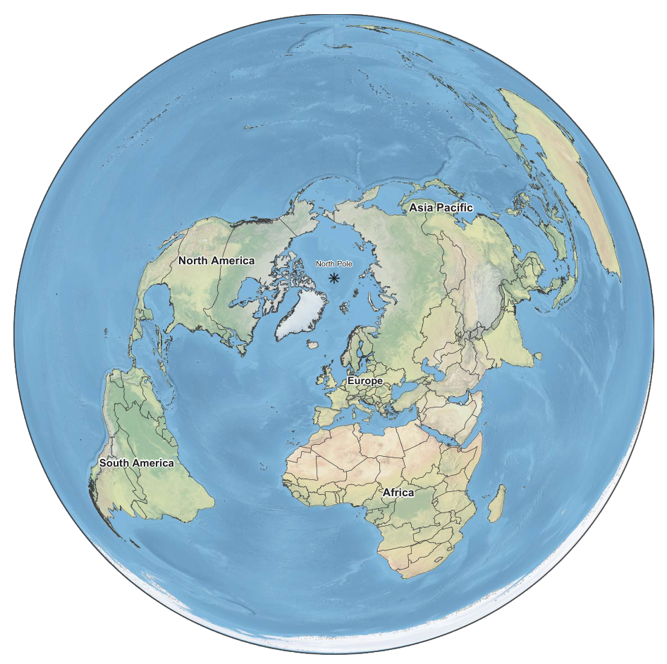
Figure 2.
African comparison of box-counting and divider fractal dimensions for the principal landmass borders of 54 countries. The dashed line denotes , indicating cross-method agreement, while the blue diamond identifies the African average. CAR (Central African Republic), DRC (Democratic Republic of the Congo), EG (Equatorial Guinea), GB (Guinea-Bissau), and STP (São Tomé and Príncipe).
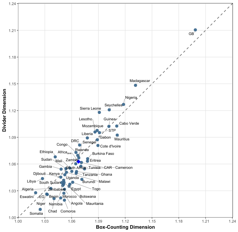
Figure 3.
Asia Pacific comparison of box-counting and divider fractal dimensions for the principal landmass borders of 63 countries. The dashed line denotes , indicating cross-method agreement, while the blue diamond identifies the Asia Pacific average. PNG (Papua New Guinea) and UAE (United Arab Emirates).
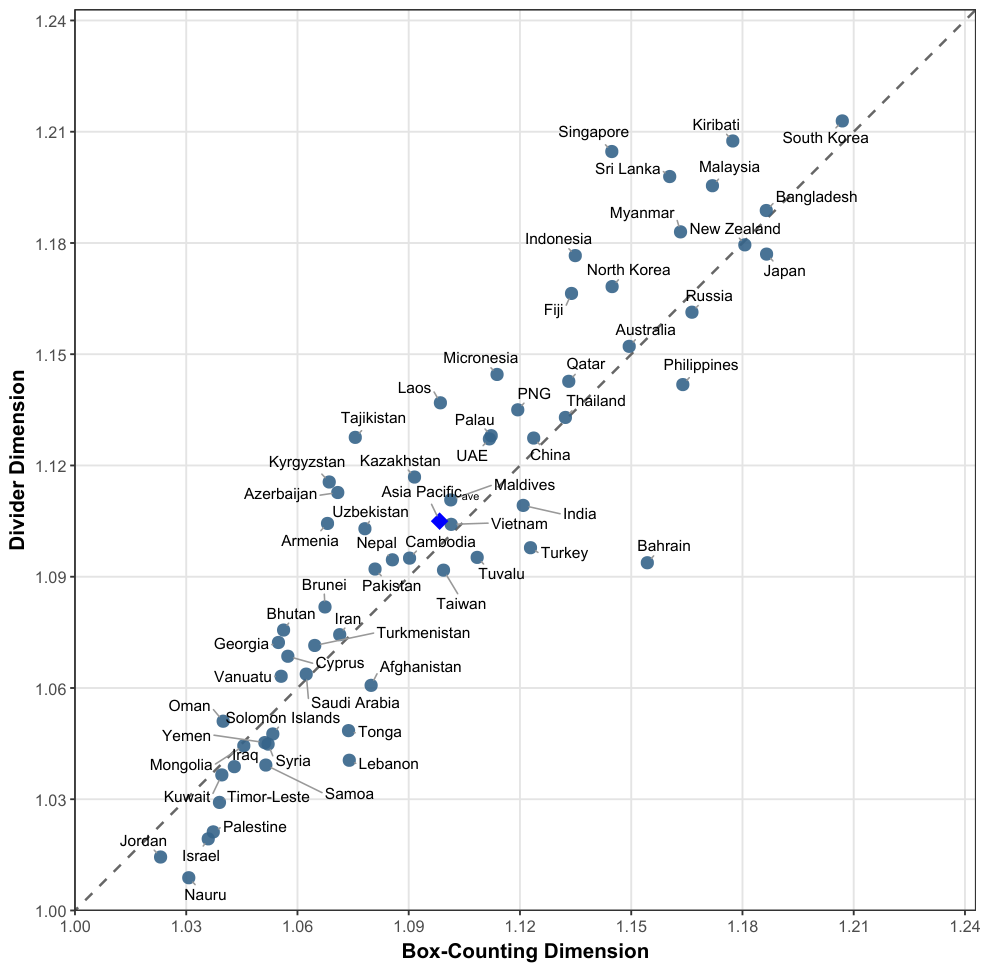
Figure 4.
European comparison of box-counting and divider fractal dimensions for the principal landmass borders of 44 countries. The dashed line denotes , indicating cross-method agreement, while the blue diamond identifies the European average. BAH (Bosnia and Herzegovina), NM (North Macedonia) and UK (United Kingdom).
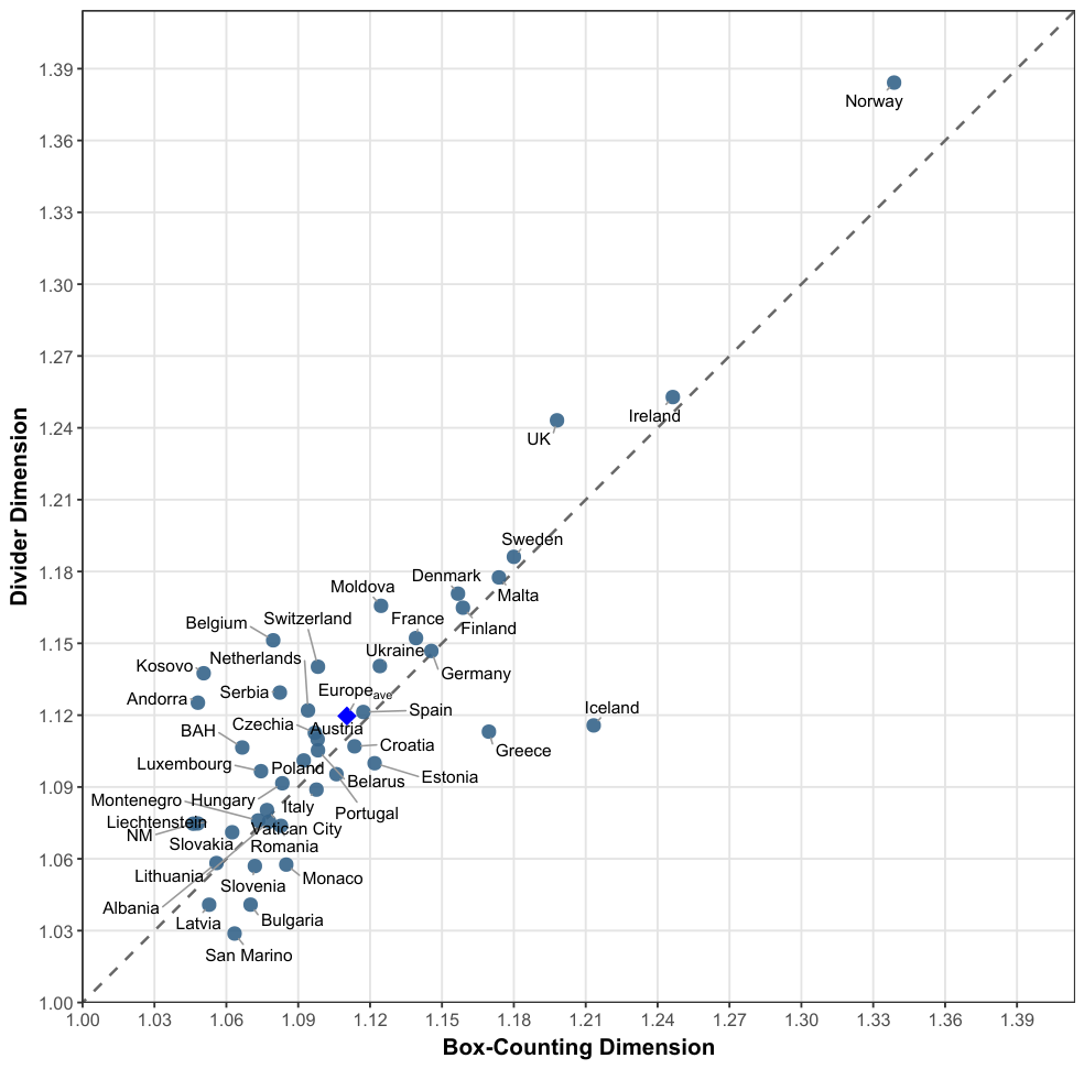
Figure 5.
North American comparison of box-counting and divider fractal dimensions for the principal landmass borders of 24 countries. The dashed line denotes , indicating cross-method agreement, while the blue diamond identifies the North American average. AAB (Antigua and Barbuda), DR (Dominican Republic), SKN (Saint Kitts and Nevis), SVG (Saint Vincent and the Grenadines), TAT (Trinidad and Tobago), and USA (United States of America).
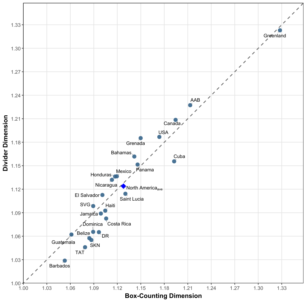
Figure 6.
South American comparison of box-counting and divider fractal dimensions for the principal landmass borders of 12 countries. The dashed line denotes , indicating cross-method agreement, while the blue diamond identifies the South American average.
Figure 6.
South American comparison of box-counting and divider fractal dimensions for the principal landmass borders of 12 countries. The dashed line denotes , indicating cross-method agreement, while the blue diamond identifies the South American average.
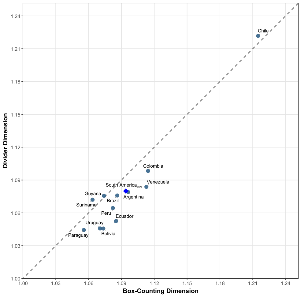
Figure 7.
Ridgeline histograms of box-counting and divider fractal-dimension estimates across the 197 countries and territories included in the study.
Figure 7.
Ridgeline histograms of box-counting and divider fractal-dimension estimates across the 197 countries and territories included in the study.
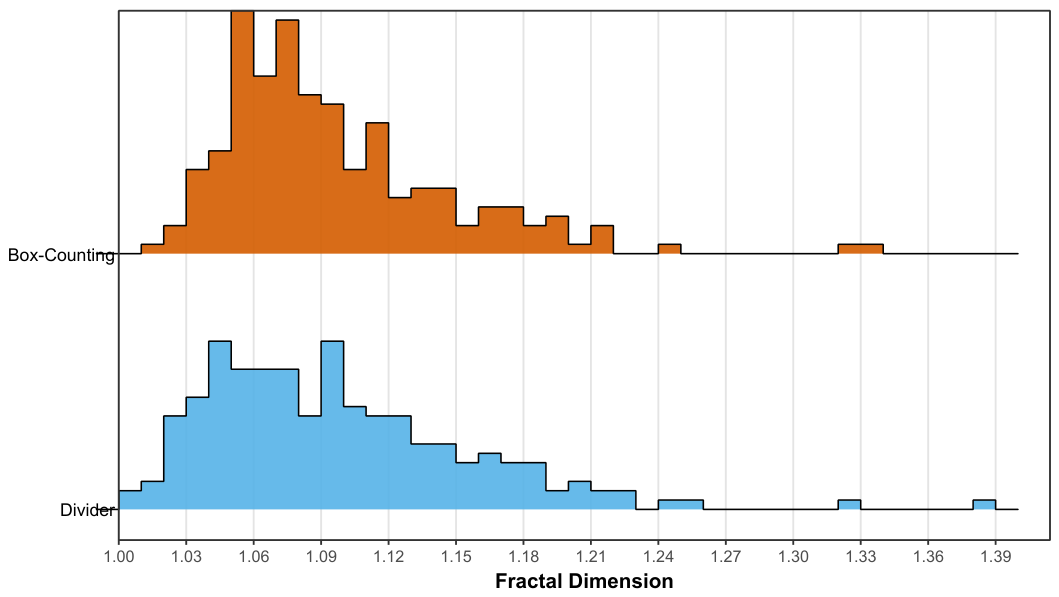
Figure 8.
Global comparison of box-counting and divider fractal dimensions for the principal landmass borders of 197 countries and territories. The dashed line denotes , indicating cross-method agreement, while the blue diamond identifies the World average.
Figure 8.
Global comparison of box-counting and divider fractal dimensions for the principal landmass borders of 197 countries and territories. The dashed line denotes , indicating cross-method agreement, while the blue diamond identifies the World average.
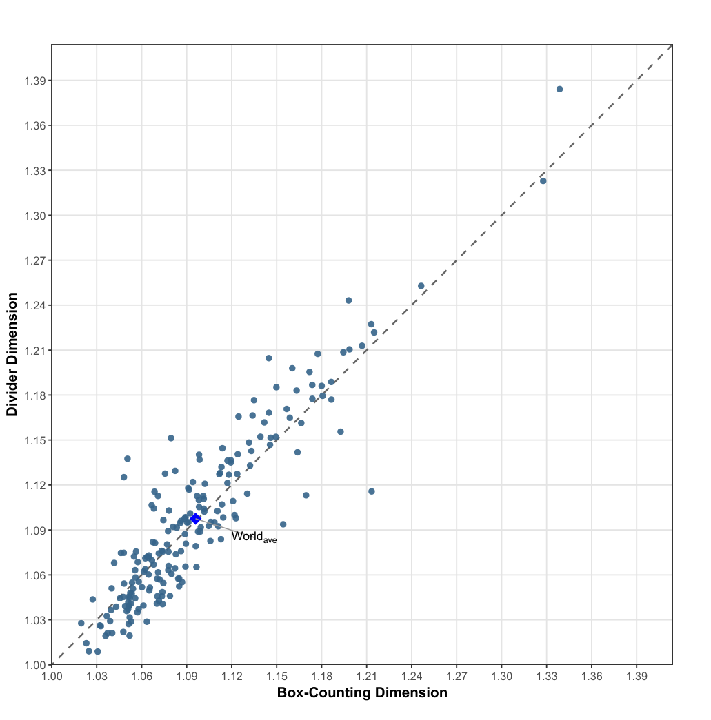
Figure 9.
Bland–Altman agreement plot comparing box-counting and divider fractal dimensions across 197 countries and territories. The solid horizontal line denotes mean bias, orange dashed lines the empirical central 95% limits, and gray dotted lines the conventional SD limits. Dotted and thin solid regression lines denote the OLS and Theil–Sen difference–magnitude trends, respectively.
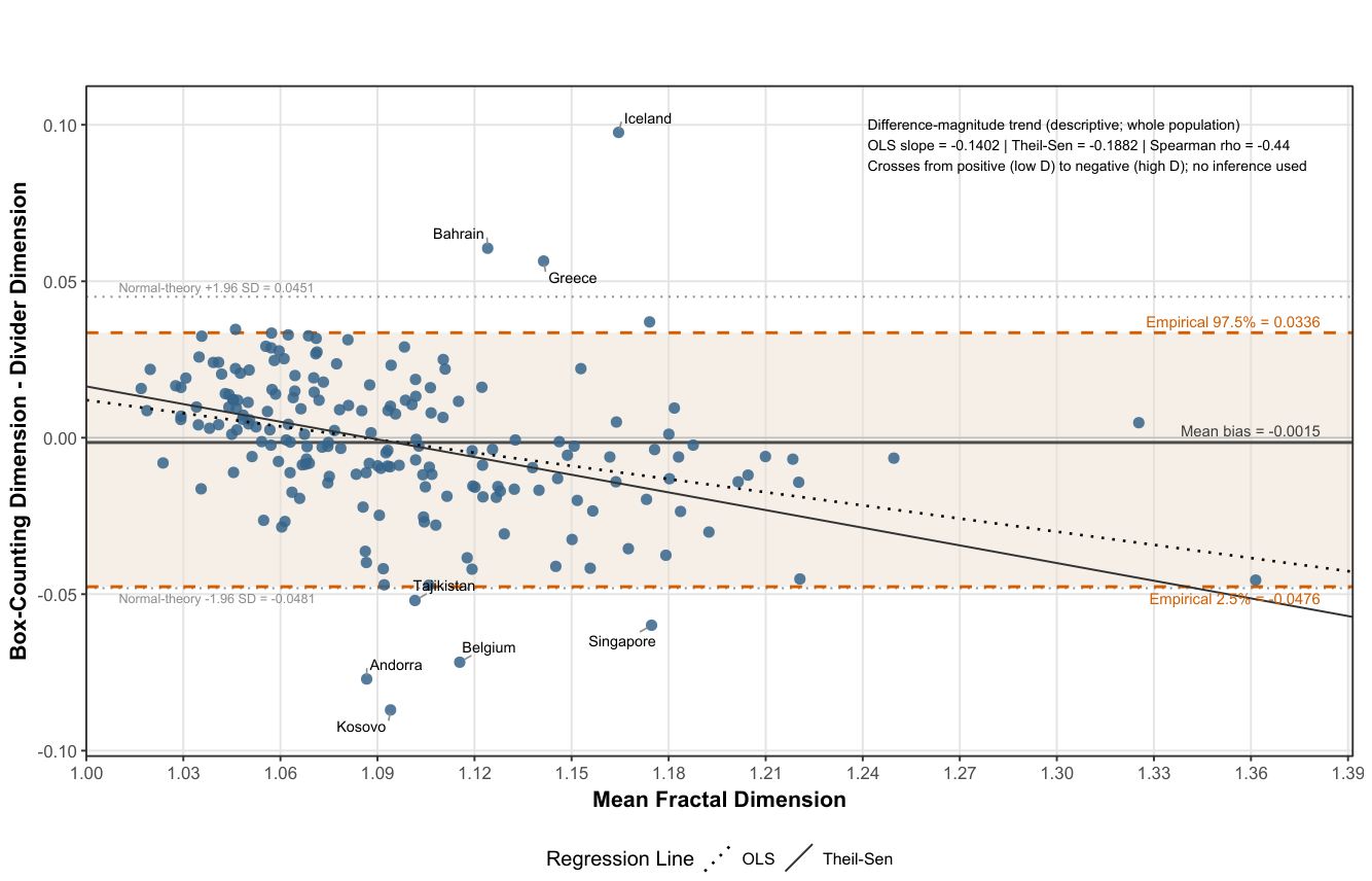
Figure 10.
Ridgeline histogram of equal-weight consensus fractal-dimension estimates across 197 countries and territories. Colored diamonds identify the corresponding continental and World averages.
Figure 10.
Ridgeline histogram of equal-weight consensus fractal-dimension estimates across 197 countries and territories. Colored diamonds identify the corresponding continental and World averages.
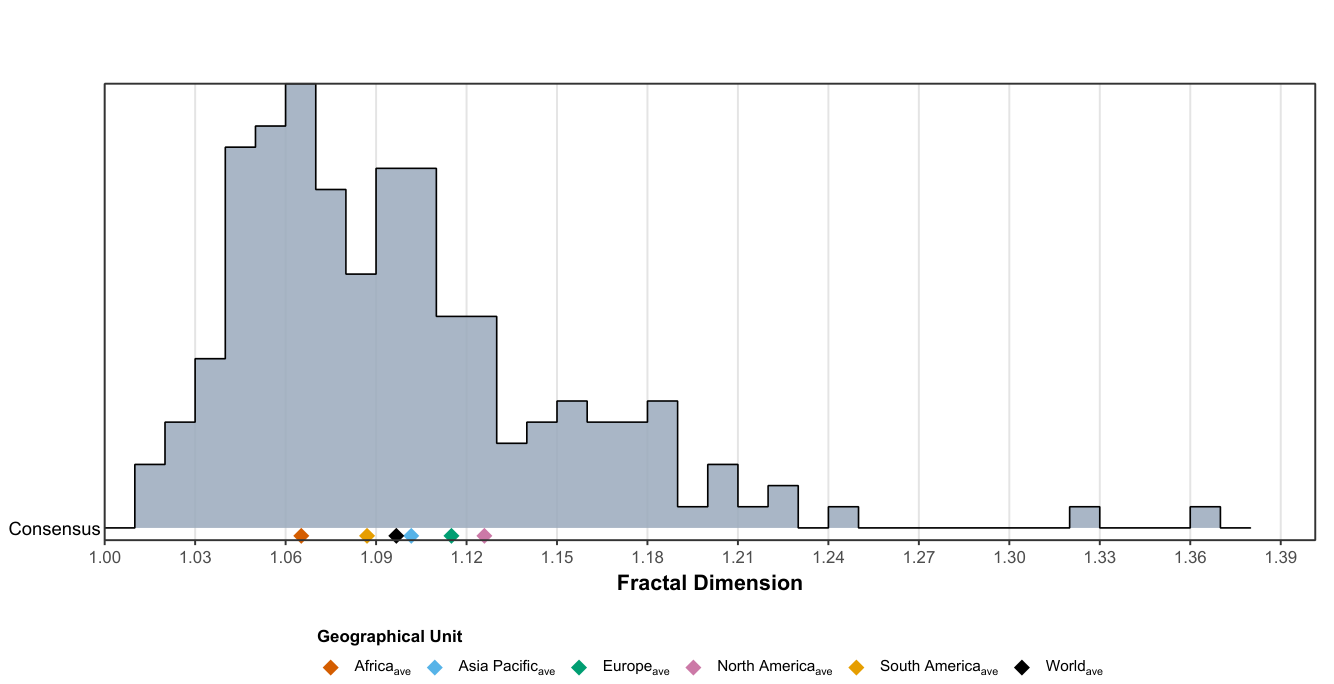
Table 1.
Fractal dimension estimations of the principal landmass borders of 54 African countries using adaptive methods.
Table 1.
Fractal dimension estimations of the principal landmass borders of 54 African countries using adaptive methods.
| Country | Fractal Dimension and its Statistics | |||||
| Box-Counting | Divider | |||||
|
Selected scale window (km) |
Selected scale window (km) |
|||||
| Algeria | 1.036694 | 0.999949 | 1.6724–200.0000 | 1.032577 | 0.986737 | 11.9913–48.9721 |
| Angola | 1.051297 | 0.999766 | 1.0960–166.9489 | 1.027231 | 0.994764 | 4.8064–38.0713 |
| Benin | 1.050011 | 0.999877 | 0.3919–42.1122 | 1.035914 | 0.992219 | 1.5510–6.1380 |
| Botswana | 1.051496 | 0.999889 | 0.8092–120.8202 | 1.039387 | 0.996223 | 1.9576–49.9434 |
| Burkina Faso | 1.077933 | 0.999576 | 0.6022–78.5622 | 1.065936 | 0.993357 | 2.5231–14.0792 |
| Burundi | 1.071477 | 0.999878 | 0.1810–25.7089 | 1.042764 | 0.994205 | 0.4340–1.8644 |
| Cabo Verde | 1.110537 | 0.999767 | 0.0750–6.3324 | 1.102601 | 0.981797 | 0.1967–2.4141 |
| Cameroon | 1.074433 | 0.999699 | 0.8485–106.9095 | 1.054554 | 0.994129 | 2.6477–34.2624 |
| CAR | 1.070958 | 0.999837 | 0.9669–121.2672 | 1.061718 | 0.994865 | 3.0138–68.6875 |
| Chad | 1.040305 | 0.999936 | 1.1562–141.4724 | 1.021243 | 0.993743 | 4.7539–19.5462 |
| Comoros | 1.051916 | 0.999892 | 0.0750–5.2572 | 1.019464 | 0.957563 | 0.3289–3.6329 |
| DRC | 1.068926 | 0.999436 | 1.7201–200.0000 | 1.081293 | 0.990209 | 28.2187–151.1928 |
| Republic of the Congo | 1.064844 | 0.999591 | 0.7303–103.5130 | 1.072984 | 0.992139 | 7.5158–57.7936 |
| Cote d’Ivoire | 1.089464 | 0.999716 | 0.5627–84.2415 | 1.080822 | 0.996480 | 2.4549–14.3808 |
| Djibouti | 1.047815 | 0.999880 | 0.1553–22.7411 | 1.045282 | 0.992966 | 1.6230–16.9599 |
| Egypt | 1.057942 | 0.999786 | 0.9042–138.3892 | 1.037304 | 0.985083 | 2.1969–56.9561 |
| Equatorial Guinea | 1.032129 | 0.999835 | 0.1529–19.7253 | 1.026301 | 0.913568 | 1.1311–19.7253 |
| Eritrea | 1.077713 | 0.999570 | 0.5485–77.9412 | 1.063151 | 0.998852 | 1.7607–10.1255 |
| Eswatini | 1.019679 | 0.999871 | 0.1258–16.7537 | 1.027739 | 0.922940 | 2.2357–16.7537 |
| Ethiopia | 1.041619 | 0.999768 | 1.1803–158.3895 | 1.068008 | 0.968306 | 21.0668–158.3895 |
| Gabon | 1.088804 | 0.999476 | 0.5412–78.7499 | 1.087219 | 0.992537 | 3.1385–43.8319 |
| Gambia | 1.048214 | 0.999551 | 0.1172–13.9810 | 1.054241 | 0.973612 | 2.1524–13.9810 |
| Ghana | 1.065468 | 0.999857 | 0.4840–61.7158 | 1.051523 | 0.995314 | 2.0144–8.3833 |
| Guinea | 1.101711 | 0.999605 | 0.5690–76.0211 | 1.102228 | 0.997060 | 2.4008–10.1296 |
| Guinea-Bissau | 1.198566 | 0.999443 | 0.2087–24.3944 | 1.210510 | 0.995564 | 1.1202–10.5290 |
| Kenya | 1.052391 | 0.999891 | 0.8001–111.4564 | 1.047971 | 0.996060 | 1.9120–111.4564 |
| Lesotho | 1.086157 | 0.999855 | 0.1920–29.1549 | 1.095931 | 0.996180 | 0.4658–8.9419 |
| Liberia | 1.077600 | 0.999834 | 0.3756–57.0093 | 1.089264 | 0.997847 | 1.6454–17.4873 |
| Libya | 1.027323 | 0.999897 | 1.2672–188.6161 | 1.043651 | 0.984340 | 32.2652–140.5308 |
| Madagascar | 1.131536 | 0.999879 | 0.8779–95.6528 | 1.148301 | 0.998038 | 0.8779–7.9829 |
| Malawi | 1.054188 | 0.999739 | 0.4464–43.5061 | 1.050719 | 0.997729 | 2.9420–11.3134 |
| Mali | 1.057998 | 0.999749 | 1.3899–200.0000 | 1.055461 | 0.984192 | 5.9939–200.0000 |
| Mauritania | 1.057156 | 0.999620 | 1.0800–156.8272 | 1.035046 | 0.990063 | 4.6699–20.1924 |
| Mauritius | 1.111079 | 0.999775 | 0.0750–8.6675 | 1.092444 | 0.989422 | 0.2106–0.8940 |
| Morocco | 1.051997 | 0.999820 | 0.8457–114.3999 | 1.031656 | 0.995204 | 2.6833–15.1656 |
| Mozambique | 1.088606 | 0.999966 | 1.1752–142.9386 | 1.097651 | 0.995647 | 1.5587–34.8261 |
| Namibia | 1.047747 | 0.999746 | 1.1250–165.0718 | 1.021952 | 0.984947 | 2.7132–28.3805 |
| Niger | 1.032731 | 0.999850 | 1.2105–163.5650 | 1.025816 | 0.954820 | 9.1268–38.6371 |
| Nigeria | 1.118096 | 0.999856 | 0.9658–132.9067 | 1.126860 | 0.992788 | 1.2903–55.7357 |
| Rwanda | 1.066820 | 0.999891 | 0.1730–24.7763 | 1.069675 | 0.986294 | 0.7451–18.5021 |
| STP | 1.091168 | 0.999678 | 0.0500–6.7347 | 1.095208 | 0.995988 | 0.3685–1.3138 |
| Senegal | 1.067997 | 0.999776 | 0.4647–60.5229 | 1.066889 | 0.993297 | 1.9461–60.5229 |
| Seychelles | 1.102120 | 0.999311 | 0.0500–3.8646 | 1.120830 | 0.986047 | 0.3453–2.3840 |
| Sierra Leone | 1.091023 | 0.999694 | 0.2757–41.7830 | 1.117915 | 0.992243 | 3.9339–17.2259 |
| Somalia | 1.024825 | 0.999958 | 1.0772–144.1166 | 1.009101 | 0.925076 | 3.4090–14.3894 |
| South Africa | 1.060186 | 0.999966 | 1.2328–175.9541 | 1.051788 | 0.996175 | 1.6506–73.3152 |
| South Sudan | 1.048969 | 0.999774 | 0.9142–120.9314 | 1.039178 | 0.994696 | 3.8459–21.5660 |
| Sudan | 1.053575 | 0.999627 | 1.3845–200.0000 | 1.054824 | 0.996640 | 10.7297–62.0659 |
| Tanzania | 1.065103 | 0.999912 | 0.9860–148.6798 | 1.049696 | 0.993679 | 2.3895–61.3529 |
| Togo | 1.061154 | 0.999872 | 0.2820–26.8291 | 1.039522 | 0.992632 | 0.8237–4.1115 |
| Tunisia | 1.070344 | 0.999863 | 0.4465–47.4122 | 1.057533 | 0.988662 | 1.7610–12.0226 |
| Uganda | 1.051064 | 0.999872 | 0.5046–75.5281 | 1.041763 | 0.980128 | 2.2015–41.8997 |
| Zambia | 1.064591 | 0.999628 | 0.9603–135.4997 | 1.060289 | 0.994893 | 9.8616–56.5728 |
| Zimbabwe | 1.050980 | 0.999670 | 0.6460–94.4250 | 1.037177 | 0.992763 | 3.7522–29.2216 |
| Average | 1.067675 | 0.999767 | 0.6879–92.7551 | 1.062706 | 0.986310 | 4.2473–37.8658 |
Notes. denotes the estimated fractal dimension and the coefficient of determination. Estimates and are reported to six decimal places; selected scale windows (km), reported to four decimals, indicate the ranges retained for regression. The Africa average is the arithmetic mean across the 54 country-level estimates; for the selected scale windows, the lower and upper limits are the arithmetic means of the corresponding country-level bounds. CAR: Central African Republic; DRC: Democratic Republic of Congo; STP: Sao Tome and Principe.
Table 2.
Fractal dimension estimations of the principal landmass borders of 63 Asia Pacific countries using adaptive methods.
Table 2.
Fractal dimension estimations of the principal landmass borders of 63 Asia Pacific countries using adaptive methods.
| Country | Fractal Dimension and its Statistics | |||||
| Box-Counting | Divider | |||||
|
Selected scale window (km) |
Selected scale window (km) |
|||||
| Afghanistan | 1.079860 | 0.999221 | 0.9373–126.4500 | 1.060715 | 0.990907 | 5.2924–22.3943 |
| Armenia | 1.068096 | 0.999374 | 0.2224–33.8644 | 1.104379 | 0.974999 | 1.7612–25.1971 |
| Azerbaijan | 1.070865 | 0.998953 | 0.3432–48.7605 | 1.112715 | 0.992843 | 4.7330–27.2167 |
| Bahrain | 1.154335 | 0.999391 | 0.0500–7.0528 | 1.093777 | 0.992219 | 0.2603–1.9548 |
| Bangladesh | 1.186413 | 0.999341 | 0.4560–59.7500 | 1.188767 | 0.997486 | 4.5227–25.2750 |
| Bhutan | 1.056248 | 0.999695 | 0.1957–21.4324 | 1.075629 | 0.992531 | 1.3531–21.4324 |
| Brunei | 1.067418 | 0.999713 | 0.0779–17.8418 | 1.081860 | 0.996188 | 1.0472–3.4129 |
| Cambodia | 1.090219 | 0.999797 | 0.4263–59.4326 | 1.095023 | 0.995564 | 2.4351–24.8664 |
| China | 1.123691 | 0.999914 | 3.5233–200.0000 | 1.127403 | 0.997752 | 5.6665–124.3564 |
| Cyprus | 1.057399 | 0.999754 | 0.0750–10.6337 | 1.068564 | 0.987749 | 0.9946–6.9117 |
| Georgia | 1.054861 | 0.999724 | 0.3228–35.3439 | 1.072276 | 0.988346 | 2.2319–35.3439 |
| India | 1.120871 | 0.999881 | 2.4225–200.0000 | 1.109242 | 0.997464 | 3.1406–54.6104 |
| Indonesia | 1.134906 | 0.999760 | 0.8455–118.6646 | 1.176603 | 0.997422 | 3.6194–118.6646 |
| Iran | 1.071385 | 0.999860 | 1.3980–200.0000 | 1.074387 | 0.992007 | 4.4945–83.2994 |
| Iraq | 1.042969 | 0.999890 | 0.7537–114.9590 | 1.038794 | 0.994275 | 4.4442–19.4962 |
| Israel | 1.035935 | 0.999599 | 0.2100–19.2693 | 1.019325 | 0.974164 | 1.0348–3.9097 |
| Japan | 1.186492 | 0.999890 | 0.7781–113.6344 | 1.177008 | 0.997967 | 0.7781–113.6344 |
| Jordan | 1.023079 | 0.999877 | 0.3589–51.9621 | 1.014423 | 0.995456 | 3.7304–16.1166 |
| Kazakhstan | 1.091558 | 0.999769 | 1.8087–200.0000 | 1.116889 | 0.990501 | 7.2183–200.0000 |
| Kuwait | 1.039596 | 0.999940 | 0.1457–21.6153 | 1.036569 | 0.963904 | 1.1417–12.0037 |
| Kyrgyzstan | 1.068560 | 0.999642 | 0.5249–56.0635 | 1.115557 | 0.992666 | 4.7286–56.0635 |
| Laos | 1.098538 | 0.999609 | 0.7119–99.9464 | 1.136904 | 0.994711 | 13.0488–99.9464 |
| Lebanon | 1.073964 | 0.999821 | 0.1306–17.6159 | 1.040518 | 0.996443 | 0.3103–1.3130 |
| Malaysia | 1.171894 | 0.999714 | 0.7018–85.4424 | 1.195451 | 0.996250 | 1.2347–85.4424 |
| Maldives | 1.101336 | 0.998118 | 0.0250–1.0199 | 1.110726 | 0.831440 | 0.3917–0.9049 |
| Mongolia | 1.045519 | 0.999810 | 1.3759–148.3755 | 1.044423 | 0.994867 | 7.1784–28.4385 |
| Myanmar | 1.163295 | 0.999916 | 1.1311–116.7287 | 1.182999 | 0.997025 | 1.9516–67.6509 |
| Nepal | 1.085601 | 0.999751 | 0.4916–56.5903 | 1.094567 | 0.993690 | 1.9852–56.5903 |
| North Korea | 1.144844 | 0.999887 | 0.4643–68.1995 | 1.168245 | 0.997953 | 1.5020–15.7193 |
| Oman | 1.039957 | 0.999967 | 0.7089–102.0364 | 1.051045 | 0.972647 | 5.4859–23.6593 |
| Pakistan | 1.080913 | 0.999818 | 1.2512–184.9752 | 1.092082 | 0.994432 | 5.4387–57.0917 |
| Palestine | 1.037288 | 0.999691 | 0.2878–10.9137 | 1.021200 | 0.944402 | 2.2466–4.9516 |
| Philippines | 1.163911 | 0.999200 | 0.4650–59.9479 | 1.141825 | 0.998435 | 0.8237–45.0442 |
| Qatar | 1.133153 | 0.999424 | 0.0910–14.7700 | 1.142704 | 0.990020 | 0.4284–14.7700 |
| Russia | 1.166369 | 0.999812 | 5.3572–200.0000 | 1.161340 | 0.997494 | 6.6285–130.6406 |
| Saudi Arabia | 1.062353 | 0.999899 | 1.5783–200.0000 | 1.063749 | 0.992290 | 3.7092–27.2368 |
| Singapore | 1.144758 | 0.998664 | 0.0500–5.5782 | 1.204666 | 0.985910 | 0.4488–4.0284 |
| South Korea | 1.206917 | 0.999657 | 0.3153–38.9417 | 1.212919 | 0.995715 | 0.9792–16.6452 |
| Sri Lanka | 1.160377 | 0.999739 | 0.2640–30.1483 | 1.197921 | 0.995318 | 4.2851–30.1483 |
| Syria | 1.052083 | 0.999791 | 0.4736–69.7370 | 1.044873 | 0.978341 | 2.7581–69.7370 |
| Taiwan | 1.099374 | 0.999918 | 0.2247–25.1022 | 1.091778 | 0.994783 | 0.3913–1.5665 |
| Tajikistan | 1.075584 | 0.999475 | 0.4681–60.6696 | 1.127588 | 0.995304 | 8.1859–45.5721 |
| Thailand | 1.132250 | 0.999877 | 0.9836–110.4002 | 1.132963 | 0.997153 | 1.7140–36.3566 |
| Timor-Leste | 1.038967 | 0.999927 | 0.1480–15.7472 | 1.029148 | 0.985622 | 1.3308–11.9666 |
| Türkiye | 1.122832 | 0.999791 | 0.8724–87.1646 | 1.097833 | 0.998613 | 3.3795–13.0909 |
| Turkmenistan | 1.064653 | 0.999901 | 0.8297–105.9690 | 1.071477 | 0.995071 | 4.5951–45.0281 |
| UAE | 1.111749 | 0.999907 | 0.3518–47.7535 | 1.127179 | 0.996709 | 0.8368–20.0742 |
| Uzbekistan | 1.078185 | 0.999435 | 0.9518–118.1538 | 1.102957 | 0.994284 | 9.2028–37.9986 |
| Vietnam | 1.101448 | 0.999692 | 0.9209–96.8893 | 1.104130 | 0.994888 | 3.6219–96.8893 |
| Yemen | 1.051196 | 0.999971 | 0.7297–88.7310 | 1.045285 | 0.984895 | 2.9947–50.4416 |
| Australia | 1.149449 | 0.999880 | 2.9159–200.0000 | 1.152129 | 0.997222 | 2.9159–121.6184 |
| Fiji | 1.133891 | 0.999601 | 0.1048–13.3522 | 1.166402 | 0.987587 | 0.4360–13.3522 |
| Kiribati | 1.177382 | 0.998853 | 0.0500–7.8801 | 1.207513 | 0.987592 | 0.8315–7.8801 |
| Micronesia | 1.113815 | 0.998546 | 0.0500–2.7180 | 1.144554 | 0.985567 | 0.3686–1.0010 |
| Nauru | 1.030682 | 0.999694 | 0.0250–1.3860 | 1.008844 | 0.962325 | 0.1347–0.7253 |
| New Zealand | 1.180630 | 0.999869 | 0.5395–79.7398 | 1.179499 | 0.995950 | 1.3028–13.6743 |
| Palau | 1.112240 | 0.998892 | 0.0500–4.0713 | 1.128042 | 0.978324 | 0.4895–3.4591 |
| PNG | 1.119402 | 0.999923 | 0.8125–112.0267 | 1.135014 | 0.996271 | 1.4506–26.3065 |
| Samoa | 1.051464 | 0.999853 | 0.0750–6.7206 | 1.039221 | 0.982108 | 0.4355–6.7206 |
| Solomon Islands | 1.053345 | 0.999838 | 0.0750–12.8469 | 1.047609 | 0.989219 | 0.5612–8.2141 |
| Tonga | 1.073765 | 0.998720 | 0.0500–3.3437 | 1.048508 | 0.948533 | 0.5262–1.4427 |
| Tuvalu | 1.108457 | 0.998525 | 0.0250–0.8676 | 1.095225 | 0.973850 | 0.0815–0.8676 |
| Vanuatu | 1.055595 | 0.999657 | 0.0750–12.8811 | 1.063166 | 0.987239 | 0.8789–6.5833 |
| Average | 1.098320 | 0.999603 | 0.6838–70.5097 | 1.104986 | 0.986649 | 2.7322–37.2532 |
Notes. denotes the estimated fractal dimension and the coefficient of determination. Estimates and are reported to six decimal places; selected scale windows (km), reported to four decimals, indicate the ranges retained for regression. The Asia Pacific average is the arithmetic mean across the 63 country-level estimates; for the selected scale windows, the lower and upper limits are the arithmetic means of the corresponding country-level bounds. Marshall Islands is excluded from the final dataset and regional average. UAE: United Arab Emirates; PNG: Papua New Guinea.
Table 3.
Fractal dimension estimations of the principal landmass borders of 44 European countries using adaptive methods.
Table 3.
Fractal dimension estimations of the principal landmass borders of 44 European countries using adaptive methods.
| Country | Fractal Dimension and its Statistics | |||||
| Box-Counting | Divider | |||||
|
Selected scale window (km) |
Selected scale window (km) |
|||||
| Albania | 1.055877 | 0.999559 | 0.1823–18.6383 | 1.058244 | 0.986093 | 1.2254–8.2370 |
| Andorra | 1.048123 | 0.999606 | 0.0500–4.9431 | 1.125213 | 0.932254 | 0.9018–2.5029 |
| Austria | 1.098112 | 0.999718 | 0.3358–36.8845 | 1.109937 | 0.996442 | 1.3375–27.9769 |
| Belarus | 1.098243 | 0.999556 | 0.4837–67.7609 | 1.105336 | 0.991542 | 2.7679–28.3274 |
| Belgium | 1.079554 | 0.999554 | 0.2010–27.8474 | 1.151283 | 0.992273 | 4.8859–27.8474 |
| BAH | 1.066639 | 0.999506 | 0.2490–37.6250 | 1.106507 | 0.995284 | 4.7661–20.8497 |
| Bulgaria | 1.070105 | 0.999850 | 0.3377–41.8147 | 1.040881 | 0.997136 | 0.7903–3.2610 |
| Croatia | 1.113490 | 0.999552 | 0.3528–50.0988 | 1.106995 | 0.996090 | 1.5155–8.7136 |
| Czechia | 1.096945 | 0.999692 | 0.3004–34.8029 | 1.112643 | 0.996675 | 1.6074–26.3152 |
| Denmark | 1.156677 | 0.998862 | 0.1745–22.4842 | 1.170751 | 0.995959 | 1.7168–7.1674 |
| Estonia | 1.121886 | 0.999734 | 0.2098–30.0631 | 1.099938 | 0.998988 | 0.5039–2.9063 |
| Finland | 1.158747 | 0.999953 | 0.6449–68.2195 | 1.164891 | 0.997878 | 1.1161–22.7815 |
| France | 1.139167 | 0.999872 | 0.7900–120.2361 | 1.152198 | 0.996988 | 2.5772–36.8580 |
| Germany | 1.145563 | 0.999583 | 0.6092–80.1803 | 1.146828 | 0.997759 | 3.4101–19.0876 |
| Greece | 1.169580 | 0.998439 | 0.4737–70.2444 | 1.113114 | 0.999458 | 1.5359–6.6821 |
| Hungary | 1.083362 | 0.999725 | 0.3289–39.5819 | 1.091560 | 0.994777 | 1.3457–12.8226 |
| Iceland | 1.213310 | 0.998721 | 0.3479–44.1178 | 1.115734 | 0.996377 | 0.2221–2.4332 |
| Ireland | 1.246342 | 0.999503 | 0.2977–38.0091 | 1.252866 | 0.995274 | 1.2394–21.4837 |
| Italy | 1.097612 | 0.999729 | 0.8117–121.7785 | 1.088911 | 0.994853 | 1.9652–37.4562 |
| Kosovo | 1.050537 | 0.999443 | 0.1240–18.5812 | 1.137520 | 0.982042 | 3.1714–18.5812 |
| Latvia | 1.052822 | 0.999848 | 0.2834–33.4941 | 1.040849 | 0.997340 | 0.6579–3.5454 |
| Liechtenstein | 1.048020 | 0.999530 | 0.0500–2.4824 | 1.074781 | 0.895726 | 0.6754–2.4824 |
| Lithuania | 1.077850 | 0.999758 | 0.2635–35.6284 | 1.075533 | 0.995369 | 1.1157–14.9875 |
| Luxembourg | 1.074459 | 0.999511 | 0.0750–9.4281 | 1.096611 | 0.993325 | 0.7570–2.6716 |
| Malta | 1.173767 | 0.998322 | 0.0500–4.2903 | 1.177546 | 0.998535 | 0.3617–0.8248 |
| Moldova | 1.124562 | 0.999504 | 0.2450–33.4556 | 1.165672 | 0.997518 | 2.4775–14.0491 |
| Monaco | 1.085004 | 0.998186 | 0.0250–0.6109 | 1.057603 | 0.981151 | 0.0250–0.3291 |
| Montenegro | 1.073280 | 0.999559 | 0.1391–19.0301 | 1.076039 | 0.991989 | 1.4077–5.9814 |
| Netherlands | 1.094079 | 0.999172 | 0.2295–32.3033 | 1.121995 | 0.998693 | 2.3543–18.0507 |
| NM | 1.046162 | 0.999339 | 0.1527–20.5768 | 1.074673 | 0.990687 | 2.7324–20.5768 |
| Norway | 1.338704 | 0.999308 | 1.0844–152.6949 | 1.384196 | 0.996062 | 6.2163–114.1392 |
| Poland | 1.092300 | 0.999765 | 0.5437–80.3315 | 1.101099 | 0.994607 | 3.1701–59.8780 |
| Portugal | 1.105954 | 0.999772 | 0.3286–35.2462 | 1.095356 | 0.996981 | 1.2997–5.1410 |
| Romania | 1.082765 | 0.999812 | 0.5043–64.7167 | 1.073803 | 0.997914 | 0.8927–20.6507 |
| San Marino | 1.063432 | 0.998701 | 0.0250–2.2771 | 1.028807 | 0.986185 | 0.3433–0.7108 |
| Serbia | 1.082321 | 0.999162 | 0.3120–41.4213 | 1.129443 | 0.994033 | 4.1508–23.3051 |
| Slovakia | 1.062440 | 0.999847 | 0.2419–26.0303 | 1.071099 | 0.993119 | 0.9578–26.0303 |
| Slovenia | 1.071906 | 0.999413 | 0.1628–20.1796 | 1.057001 | 0.980734 | 0.8922–4.8894 |
| Spain | 1.117171 | 0.999957 | 0.7757–109.0026 | 1.121330 | 0.995658 | 1.0375–45.5427 |
| Sweden | 1.179988 | 0.999892 | 0.8274–84.2649 | 1.186140 | 0.996946 | 0.8274–64.1997 |
| Switzerland | 1.098226 | 0.999331 | 0.2269–27.6417 | 1.140230 | 0.998344 | 2.1744–20.8388 |
| Ukraine | 1.124068 | 0.999691 | 0.8844–110.8476 | 1.140512 | 0.995541 | 3.6621–62.7904 |
| UK | 1.198006 | 0.999304 | 0.5794–65.1326 | 1.243138 | 0.998317 | 5.3463–28.3063 |
| Vatican City | 1.076956 | 0.998609 | 0.0250–0.2066 | 1.080362 | 0.921951 | 0.0250–0.1119 |
| Average | 1.110321 | 0.999442 | 0.3486–45.1183 | 1.119663 | 0.989111 | 1.8673–20.5074 |
Notes. denotes the estimated fractal dimension and the coefficient of determination. Estimates and are reported to six decimal places; selected scale windows (km), reported to four decimals, indicate the ranges retained for regression. The Europe average is the arithmetic mean across the 44 country-level estimates; for the selected scale windows, the lower and upper limits are the arithmetic means of the corresponding country-level bounds. BAH: Bosnia and Herzegovina; NM: North Macedonia; UK: United Kingdom.
Table 4.
Fractal dimension estimations of the principal landmass borders of 24 North American countries and territories using adaptive methods
Table 4.
Fractal dimension estimations of the principal landmass borders of 24 North American countries and territories using adaptive methods
| Country/Territory | Fractal Dimension and its Statistics | |||||
|---|---|---|---|---|---|---|
| Box-Counting | Divider | |||||
|
Selected scale window (km) |
Selected scale window (km) |
|||||
| AAB | 1.213096 | 0.998104 | 0.0588–3.8981 | 1.227321 | 0.988662 | 0.2136–3.8981 |
| Bahamas | 1.141743 | 0.999670 | 0.0750–12.6086 | 1.161767 | 0.991225 | 0.4458–5.1714 |
| Barbados | 1.052942 | 0.999833 | 0.0500–5.0158 | 1.028839 | 0.940516 | 0.2323–0.5454 |
| Belize | 1.084338 | 0.999907 | 0.1524–15.1101 | 1.057509 | 0.992926 | 0.5890–2.2765 |
| Canada | 1.194451 | 0.999923 | 3.3987–200.0000 | 1.208539 | 0.997441 | 3.3987–123.8305 |
| Costa Rica | 1.105798 | 0.999625 | 0.2955–43.9716 | 1.082625 | 0.998842 | 1.2869–5.6047 |
| Cuba | 1.192614 | 0.999881 | 0.5294–46.7350 | 1.155604 | 0.998673 | 0.6891–4.3601 |
| Dominica | 1.089183 | 0.999554 | 0.0500–5.1511 | 1.065570 | 0.984838 | 0.2783–2.1834 |
| DR | 1.096513 | 0.999566 | 0.2582–32.1883 | 1.065206 | 0.995993 | 0.8038–3.3228 |
| El Salvador | 1.100978 | 0.999790 | 0.1581–17.9279 | 1.112671 | 0.992769 | 1.4647–7.7791 |
| Greenland | 1.327729 | 0.999657 | 1.6131–183.1275 | 1.322921 | 0.996238 | 8.5701–45.5316 |
| Grenada | 1.149821 | 0.999213 | 0.0500–4.3605 | 1.185281 | 0.991980 | 0.1418–3.8506 |
| Guatemala | 1.061448 | 0.999877 | 0.3595–53.6933 | 1.062157 | 0.983639 | 1.5675–53.6933 |
| Haiti | 1.104640 | 0.999854 | 0.2073–26.7042 | 1.092664 | 0.996203 | 0.6503–4.8072 |
| Honduras | 1.117207 | 0.999642 | 0.3878–42.0784 | 1.136249 | 0.996903 | 3.5194–24.2434 |
| Jamaica | 1.099034 | 0.999798 | 0.1025–15.1309 | 1.088956 | 0.992234 | 0.3773–15.1309 |
| Mexico | 1.119433 | 0.999676 | 2.0256–200.0000 | 1.136494 | 0.997500 | 2.6538–30.1838 |
| Nicaragua | 1.113157 | 0.999874 | 0.3956–59.7761 | 1.132050 | 0.993659 | 2.3251–33.1243 |
| Panama | 1.145922 | 0.999879 | 0.3421–33.6221 | 1.151507 | 0.996871 | 0.7687–11.4238 |
| SKN | 1.086919 | 0.999517 | 0.0500–4.5620 | 1.055165 | 0.971694 | 0.2661–1.6733 |
| Saint Lucia | 1.130345 | 0.999206 | 0.0500–4.5452 | 1.114211 | 0.995144 | 0.1902–0.5182 |
| SVG | 1.089244 | 0.999760 | 0.0500–3.5765 | 1.098521 | 0.977278 | 0.2848–0.7356 |
| TAT | 1.078840 | 0.999816 | 0.0750–14.7736 | 1.045974 | 0.988558 | 0.4711–3.7234 |
| USA | 1.173701 | 0.999835 | 2.9825–200.0000 | 1.186805 | 0.998193 | 2.9825–74.3492 |
| Average | 1.127879 | 0.999644 | 0.5715–51.1899 | 1.123942 | 0.989916 | 1.4238–19.2484 |
Notes. denotes the estimated fractal dimension and the coefficient of determination. Estimates and are reported to six decimal places; selected scale windows (km), reported to four decimals, indicate the ranges retained for regression. The North America average is the arithmetic mean across the 24 country- and territory-level estimates; for the selected scale windows, the lower and upper limits are the arithmetic means of the corresponding bounds. AAB: Antigua and Barbuda; DR: Dominican Republic; SKN: Saint Kitts and Nevis; SVG: Saint Vincent and the Grenadines; TAT: Trinidad and Tobago; USA: United States of America.
Table 5.
Fractal dimension estimations of the principal landmass borders of 12 South American countries using adaptive methods
Table 5.
Fractal dimension estimations of the principal landmass borders of 12 South American countries using adaptive methods
| Country | Fractal Dimension and its Statistics | |||||
|---|---|---|---|---|---|---|
| Box-Counting | Divider | |||||
|
Selected scale window (km) |
Selected scale window (km) |
|||||
| Argentina | 1.096022 | 0.999837 | 1.9774–200.0000 | 1.079149 | 0.997393 | 2.5943–116.1861 |
| Bolivia | 1.073454 | 0.999852 | 1.1298–162.9843 | 1.045705 | 0.996445 | 2.7167–15.7067 |
| Brazil | 1.086192 | 0.999977 | 3.5307–200.0000 | 1.075879 | 0.995946 | 4.4771–200.0000 |
| Chile | 1.214958 | 0.999816 | 1.4497–97.6034 | 1.221808 | 0.997566 | 3.9033–97.6034 |
| Colombia | 1.114353 | 0.999816 | 1.2910–169.3581 | 1.098356 | 0.995664 | 1.7200–53.7631 |
| Ecuador | 1.084970 | 0.999736 | 0.5566–81.0092 | 1.052404 | 0.995747 | 1.3405–7.7745 |
| Guyana | 1.074082 | 0.999580 | 0.5435–68.0903 | 1.075585 | 0.994557 | 3.9722–16.4458 |
| Paraguay | 1.055658 | 0.999793 | 0.7256–107.1781 | 1.044361 | 0.997034 | 3.1533–79.8905 |
| Peru | 1.082176 | 0.999952 | 1.3732–174.1817 | 1.064391 | 0.994140 | 1.8258–55.7332 |
| Suriname | 1.063588 | 0.999364 | 0.3752–57.0474 | 1.072044 | 0.999727 | 3.9910–17.4918 |
| Uruguay | 1.070442 | 0.999775 | 0.4244–62.3477 | 1.045760 | 0.993235 | 1.0238–19.2725 |
| Venezuela | 1.112835 | 0.999599 | 1.1273–159.8280 | 1.083825 | 0.994490 | 3.6165–49.8182 |
| Average | 1.094061 | 0.999758 | 1.2087–128.3024 | 1.079939 | 0.995995 | 2.8612–60.8072 |
Notes: denotes the estimated fractal dimension and R2 the coefficient of determination. Estimates and R2 are reported to six decimal places; selected scale windows (km), reported to four decimals, indicate the ranges retained for regression. The South America average is the arithmetic mean across the 12 country-level estimates; for the selected scale windows, the lower and upper limits are the arithmetic means of the corresponding country-level bounds.
Table 6.
Descriptive statistical analysis of border fractal dimensions across the 197 countries and territories included in the World Statistical Atlas ().
Table 6.
Descriptive statistical analysis of border fractal dimensions across the 197 countries and territories included in the World Statistical Atlas ().
| Statistic | |||
|---|---|---|---|
| (a) Descriptive statistics | |||
| Median (Q1, Q3) | 1.0834 (1.0580, 1.1181) | 1.0890 (1.0524, 1.1280) | |
| Mean (Min, Max) | 1.0959 (1.0197, 1.3387) | 1.0975 (1.0088, 1.3842) | |
| SD (SE) | 0.0513 (0.0037) | 0.0587 (0.0042) | |
| IQR (Q3 - Q1) | 0.0601 | 0.0756 | |
| RSE (%) | 0.33% | 0.38% | |
| (%) | 9.59% | 9.75% | |
| (b) Distribution shape statistics | |||
| Adjusted skewness | 1.5665 | 1.2962 | |
| Excess kurtosis | 3.7805 | 2.9151 | |
| Shapiro–Wilk W (p) | 0.8839 () | 0.9169 () | |
| IQR outliers, n (%) | 6 (3.05%) | 4 (2.03%) | |
| (c) One-sample Tests: . | |||
| t-test | |||
| (95% CI) | 1.0959 (1.0899, ) | 1.0975 (1.0905, ) | |
| Sig. (1-sided) | |||
| Wilcoxon test | |||
| (95% CI) | 1.0893 (1.0837, ) | 1.0921 (1.0853, ) | |
| Sig. (1-sided) | |||
| (d) Paired-sample Tests: . | |||
| t-test | |||
| (95% CI) | (, 0.0018) | ||
| Sig. (2-sided) | 0.3715 | ||
| Wilcoxon test | |||
| (95% CI) | (, 0.0024) | ||
| Sig. (2-sided) | 0.6832 | ||
Notes. Q1 and Q3 denote the first and third quartiles; SD, SE, IQR, RSE, and PED0 are defined in the Methods Section. Panel (b) reports distribution-shape and normality diagnostics. Panel (c) reports one-sided 95% lower confidence intervals; Panel (d) reports two-sided intervals for box-counting minus divider differences. Wilcoxon estimates are Hodges–Lehmann pseudomedians; for n ≥ 50, the normal approximation is used.
Table 7.
Cross-method association and concordance between box-counting and divider fractal-dimension estimates across the 197 countries and territories included in the World Statistical Atlas ().
Table 7.
Cross-method association and concordance between box-counting and divider fractal-dimension estimates across the 197 countries and territories included in the World Statistical Atlas ().
| Statistic | Estimate | 95% CI | Sig. (2-sided) |
|---|---|---|---|
| (a) Association statistics | |||
| Pearson correlation coefficient (r) | 0.9155 | (0.8895, 0.9355) | |
| Spearman rank correlation () | 0.8789 | (0.8226, 0.9176) | |
| Kendall rank correlation () | 0.7174 | (0.6602, 0.7668) | |
| (b) Concordance statistic | |||
| Lin concordance correlation coefficient (CCC) | 0.9069 | (0.8599, 0.9371) | — |
Notes. r, ρ, τ, and CCC denote Pearson, Spearman, Kendall, and Lin concordance correlation coefficients, respectively. Pearson CI is analytical; Spearman, Kendall, and CCC CIs are percentile-bootstrap intervals based on 10,000 paired country-level resamples (seed = 123). Reported p-values are two-sided; no significance test is reported for CCC. Correlation and concordance should be interpreted jointly with the equality and paired-difference analyses.
Table 9.
Geographical Unit box-counting, divider, and consensus fractal dimensions, grouped by continent ().
Table 9.
Geographical Unit box-counting, divider, and consensus fractal dimensions, grouped by continent ().
| Geographical Unit | Geographical Unit | ||||||
| Africa | |||||||
| Algeria | 1.036694 | 1.032577 | 1.034636 | Angola | 1.051297 | 1.027231 | 1.039264 |
| Benin | 1.050011 | 1.035914 | 1.042963 | Botswana | 1.051496 | 1.039387 | 1.045442 |
| Burkina Faso | 1.077933 | 1.065936 | 1.071935 | Burundi | 1.071477 | 1.042764 | 1.057121 |
| Cabo Verde | 1.110537 | 1.102601 | 1.106569 | Cameroon | 1.074433 | 1.054554 | 1.064494 |
| CAR | 1.070958 | 1.061718 | 1.066338 | Chad | 1.040305 | 1.021243 | 1.030774 |
| Comoros | 1.051916 | 1.019464 | 1.035690 | DRC | 1.068926 | 1.081293 | 1.075110 |
| RC | 1.064844 | 1.072984 | 1.068914 | Cote d’Ivoire | 1.089464 | 1.080822 | 1.085143 |
| Djibouti | 1.047815 | 1.045282 | 1.046549 | Egypt | 1.057942 | 1.037304 | 1.047623 |
| Equatorial Guinea | 1.032129 | 1.026301 | 1.029215 | Eritrea | 1.077713 | 1.063151 | 1.070432 |
| Eswatini | 1.019679 | 1.027739 | 1.023709 | Ethiopia | 1.041619 | 1.068008 | 1.054814 |
| Gabon | 1.088804 | 1.087219 | 1.088012 | Gambia | 1.048214 | 1.054241 | 1.051228 |
| Ghana | 1.065468 | 1.051523 | 1.058496 | Guinea | 1.101711 | 1.102228 | 1.101970 |
| Guinea-Bissau | 1.198566 | 1.210510 | 1.204538 | Kenya | 1.052391 | 1.047971 | 1.050181 |
| Lesotho | 1.086157 | 1.095931 | 1.091044 | Liberia | 1.077600 | 1.089264 | 1.083432 |
| Libya | 1.027323 | 1.043651 | 1.035487 | Madagascar | 1.131536 | 1.148301 | 1.139919 |
| Malawi | 1.054188 | 1.050719 | 1.052454 | Mali | 1.057998 | 1.055461 | 1.056730 |
| Mauritania | 1.057156 | 1.035046 | 1.046101 | Mauritius | 1.111079 | 1.092444 | 1.101762 |
| Morocco | 1.051997 | 1.031656 | 1.041827 | Mozambique | 1.088606 | 1.097651 | 1.093129 |
| Namibia | 1.047747 | 1.021952 | 1.034850 | Niger | 1.032731 | 1.025816 | 1.029274 |
| Nigeria | 1.118096 | 1.126860 | 1.122478 | Rwanda | 1.066820 | 1.069675 | 1.068248 |
| STP | 1.091168 | 1.095208 | 1.093188 | Senegal | 1.067997 | 1.066889 | 1.067443 |
| Seychelles | 1.102120 | 1.120830 | 1.111475 | Sierra Leone | 1.091023 | 1.117915 | 1.104469 |
| Somalia | 1.024825 | 1.009101 | 1.016963 | South Africa | 1.060186 | 1.051788 | 1.055987 |
| South Sudan | 1.048969 | 1.039178 | 1.044074 | Sudan | 1.053575 | 1.054824 | 1.054200 |
| Tanzania | 1.065103 | 1.049696 | 1.057400 | Togo | 1.061154 | 1.039522 | 1.050338 |
| Tunisia | 1.070344 | 1.057533 | 1.063939 | Uganda | 1.051064 | 1.041763 | 1.046414 |
| Zambia | 1.064591 | 1.060289 | 1.062440 | Zimbabwe | 1.050980 | 1.037177 | 1.044079 |
| Asia Pacific | |||||||
| Afghanistan | 1.079860 | 1.060715 | 1.070288 | Armenia | 1.068096 | 1.104379 | 1.086238 |
| Azerbaijan | 1.070865 | 1.112715 | 1.091790 | Bahrain | 1.154335 | 1.093777 | 1.124056 |
| Bangladesh | 1.186413 | 1.188767 | 1.187590 | Bhutan | 1.056248 | 1.075629 | 1.065939 |
| Brunei | 1.067418 | 1.081860 | 1.074639 | Cambodia | 1.090219 | 1.095023 | 1.092621 |
| China | 1.123691 | 1.127403 | 1.125547 | Cyprus | 1.057399 | 1.068564 | 1.062982 |
| Georgia | 1.054861 | 1.072276 | 1.063569 | India | 1.120871 | 1.109242 | 1.115057 |
| Indonesia | 1.134906 | 1.176603 | 1.155755 | Iran | 1.071385 | 1.074387 | 1.072886 |
| Iraq | 1.042969 | 1.038794 | 1.040882 | Israel | 1.035935 | 1.019325 | 1.027630 |
| Japan | 1.186492 | 1.177008 | 1.181750 | Jordan | 1.023079 | 1.014423 | 1.018751 |
| Kazakhstan | 1.091558 | 1.116889 | 1.104224 | Kuwait | 1.039596 | 1.036569 | 1.038083 |
| Kyrgyzstan | 1.068560 | 1.115557 | 1.092059 | Laos | 1.098538 | 1.136904 | 1.117721 |
| Lebanon | 1.073964 | 1.040518 | 1.057241 | Malaysia | 1.171894 | 1.195451 | 1.183673 |
| Maldives | 1.101336 | 1.110726 | 1.106031 | Mongolia | 1.045519 | 1.044423 | 1.044971 |
| Myanmar | 1.163295 | 1.182999 | 1.173147 | Nepal | 1.085601 | 1.094567 | 1.090084 |
| North Korea | 1.144844 | 1.168245 | 1.156545 | Oman | 1.039957 | 1.051045 | 1.045501 |
| Pakistan | 1.080913 | 1.092082 | 1.086498 | Palestine | 1.037288 | 1.021200 | 1.029244 |
| Philippines | 1.163911 | 1.141825 | 1.152868 | Qatar | 1.133153 | 1.142704 | 1.137929 |
| Russia | 1.166369 | 1.161340 | 1.163855 | Saudi Arabia | 1.062353 | 1.063749 | 1.063051 |
| Singapore | 1.144758 | 1.204666 | 1.174712 | South Korea | 1.206917 | 1.212919 | 1.209918 |
| Sri Lanka | 1.160377 | 1.197921 | 1.179149 | Syria | 1.052083 | 1.044873 | 1.048478 |
| Taiwan | 1.099374 | 1.091778 | 1.095576 | Tajikistan | 1.075584 | 1.127588 | 1.101586 |
| Thailand | 1.132250 | 1.132963 | 1.132607 | Timor-Leste | 1.038967 | 1.029148 | 1.034058 |
| Türkiye | 1.122832 | 1.097833 | 1.110333 | Turkmenistan | 1.064653 | 1.071477 | 1.068065 |
| UAE | 1.111749 | 1.127179 | 1.119464 | Uzbekistan | 1.078185 | 1.102957 | 1.090571 |
| Vietnam | 1.101448 | 1.104130 | 1.102789 | Yemen | 1.051196 | 1.045285 | 1.048241 |
| Australia | 1.149449 | 1.152129 | 1.150789 | Fiji | 1.133891 | 1.166402 | 1.150147 |
| Kiribati | 1.177382 | 1.207513 | 1.192448 | Micronesia | 1.113815 | 1.144554 | 1.129185 |
| Nauru | 1.030682 | 1.008844 | 1.019763 | New Zealand | 1.180630 | 1.179499 | 1.180065 |
| Palau | 1.112240 | 1.128042 | 1.120141 | PNG | 1.119402 | 1.135014 | 1.127208 |
| Samoa | 1.051464 | 1.039221 | 1.045343 | Solomon Islands | 1.053345 | 1.047609 | 1.050477 |
| Tonga | 1.073765 | 1.048508 | 1.061137 | Tuvalu | 1.108457 | 1.095225 | 1.101841 |
| Vanuatu | 1.055595 | 1.063166 | 1.059381 | ||||
| Europe | |||||||
| Albania | 1.055877 | 1.058244 | 1.057061 | Andorra | 1.048123 | 1.125213 | 1.086668 |
| Austria | 1.098112 | 1.109937 | 1.104025 | Belarus | 1.098243 | 1.105336 | 1.101790 |
| Belgium | 1.079554 | 1.151283 | 1.115419 | BAH | 1.066639 | 1.106507 | 1.086573 |
| Bulgaria | 1.070105 | 1.040881 | 1.055493 | Croatia | 1.113490 | 1.106995 | 1.110243 |
| Czechia | 1.096945 | 1.112643 | 1.104794 | Denmark | 1.156677 | 1.170751 | 1.163714 |
| Estonia | 1.121886 | 1.099938 | 1.110912 | Finland | 1.158747 | 1.164891 | 1.161819 |
| France | 1.139167 | 1.152198 | 1.145683 | Germany | 1.145563 | 1.146828 | 1.146196 |
| Greece | 1.169580 | 1.113114 | 1.141347 | Hungary | 1.083362 | 1.091560 | 1.087461 |
| Iceland | 1.213310 | 1.115734 | 1.164522 | Ireland | 1.246342 | 1.252866 | 1.249604 |
| Italy | 1.097612 | 1.088911 | 1.093262 | Kosovo | 1.050537 | 1.137520 | 1.094029 |
| Latvia | 1.052822 | 1.040849 | 1.046836 | Liechtenstein | 1.048020 | 1.074781 | 1.061401 |
| Lithuania | 1.077850 | 1.075533 | 1.076692 | Luxembourg | 1.074459 | 1.096611 | 1.085535 |
| Malta | 1.173767 | 1.177546 | 1.175657 | Moldova | 1.124562 | 1.165672 | 1.145117 |
| Monaco | 1.085004 | 1.057603 | 1.071304 | Montenegro | 1.073280 | 1.076039 | 1.074660 |
| Netherlands | 1.094079 | 1.121995 | 1.108037 | NM | 1.046162 | 1.074673 | 1.060418 |
| Norway | 1.338704 | 1.384196 | 1.361450 | Poland | 1.092300 | 1.101099 | 1.096700 |
| Portugal | 1.105954 | 1.095356 | 1.100655 | Romania | 1.082765 | 1.073803 | 1.078284 |
| San Marino | 1.063432 | 1.028807 | 1.046120 | Serbia | 1.082321 | 1.129443 | 1.105882 |
| Slovakia | 1.062440 | 1.071099 | 1.066770 | Slovenia | 1.071906 | 1.057001 | 1.064454 |
| Spain | 1.117171 | 1.121330 | 1.119251 | Sweden | 1.179988 | 1.186140 | 1.183064 |
| Switzerland | 1.098226 | 1.140230 | 1.119228 | Ukraine | 1.124068 | 1.140512 | 1.132290 |
| UK | 1.198006 | 1.243138 | 1.220572 | Vatican City | 1.076956 | 1.080362 | 1.078659 |
| North America | |||||||
| AAB | 1.213096 | 1.227321 | 1.220209 | Bahamas | 1.141743 | 1.161767 | 1.151755 |
| Barbados | 1.052942 | 1.028839 | 1.040891 | Belize | 1.084338 | 1.057509 | 1.070924 |
| Canada | 1.194451 | 1.208539 | 1.201495 | Costa Rica | 1.105798 | 1.082625 | 1.094212 |
| Cuba | 1.192614 | 1.155604 | 1.174109 | Dominica | 1.089183 | 1.065570 | 1.077377 |
| DR | 1.096513 | 1.065206 | 1.080860 | El Salvador | 1.100978 | 1.112671 | 1.106825 |
| Greenland | 1.327729 | 1.322921 | 1.325325 | Grenada | 1.149821 | 1.185281 | 1.167551 |
| Guatemala | 1.061448 | 1.062157 | 1.061803 | Haiti | 1.104640 | 1.092664 | 1.098652 |
| Honduras | 1.117207 | 1.136249 | 1.126728 | Jamaica | 1.099034 | 1.088956 | 1.093995 |
| Mexico | 1.119433 | 1.136494 | 1.127964 | Nicaragua | 1.113157 | 1.132050 | 1.122604 |
| Panama | 1.145922 | 1.151507 | 1.148715 | SKN | 1.086919 | 1.055165 | 1.071042 |
| Saint Lucia | 1.130345 | 1.114211 | 1.122278 | SVG | 1.089244 | 1.098521 | 1.093883 |
| TAT | 1.078840 | 1.045974 | 1.062407 | USA | 1.173701 | 1.186805 | 1.180253 |
| South America | |||||||
| Argentina | 1.096022 | 1.079149 | 1.087586 | Bolivia | 1.073454 | 1.045705 | 1.059580 |
| Brazil | 1.086192 | 1.075879 | 1.081036 | Chile | 1.214958 | 1.221808 | 1.218383 |
| Colombia | 1.114353 | 1.098356 | 1.106355 | Ecuador | 1.084970 | 1.052404 | 1.068687 |
| Guyana | 1.074082 | 1.075585 | 1.074834 | Paraguay | 1.055658 | 1.044361 | 1.050010 |
| Peru | 1.082176 | 1.064391 | 1.073284 | Suriname | 1.063588 | 1.072044 | 1.067816 |
| Uruguay | 1.070442 | 1.045760 | 1.058101 | Venezuela | 1.112835 | 1.083825 | 1.098330 |
| Overall Averages | |||||||
| Africa | 1.067675 | 1.062706 | 1.065191 | Asia Pacific | 1.098320 | 1.104986 | 1.101653 |
| Europe | 1.110321 | 1.119663 | 1.114992 | North America | 1.127879 | 1.123942 | 1.125911 |
| South America | 1.094061 | 1.079939 | 1.087000 | World | 1.095942 | 1.097458 | 1.096700 |
Notes. The equal-weight consensus fractal dimension is DConsensus = (DBox.Counting + DDivider)/2. All estimates are reported to six decimal places; box-counting and divider values remain the primary method-specific estimates. CAR: Central African Republic; DRC: Democratic Republic of Congo; RC: Republic of Congo; STP: Sao Tome and Principe; UAE: United Arab Emirates; PNG: Papua New Guinea; BAH: Bosnia and Herzegovina; NM: North Macedonia; UK: United Kingdom; AAB: Antigua and Barbuda; DR: Dominican Republic; SKN: Saint Kitts and Nevis; SVG: Saint Vincent and the Grenadines; TAT: Trinidad and Tobago; USA: United States of America
Disclaimer/Publisher’s Note: The statements, opinions and data contained in all publications are solely those of the individual author(s) and contributor(s) and not of MDPI and/or the editor(s). MDPI and/or the editor(s) disclaim responsibility for any injury to people or property resulting from any ideas, methods, instructions or products referred to in the content. |
© 2026 by the authors. Licensee MDPI, Basel, Switzerland. This article is an open access article distributed under the terms and conditions of the Creative Commons Attribution (CC BY) license (http://creativecommons.org/licenses/by/4.0/).
Copyright: This open access article is published under a Creative Commons CC BY 4.0 license, which permit the free download, distribution, and reuse, provided that the author and preprint are cited in any reuse.