

Submitted:
14 September 2026
Posted:
15 September 2026
You are already at the latest version
Abstract
Heterogeneous multi-robot task allocation (MRTA) requires the efficient coordination of robots with different capabilities while balancing task benefits, travel costs, and completion time. To address the challenges of complex constraints and premature convergence in conventional optimization methods, this paper proposes a heterogeneous MRTA algorithm based on chaotic adaptive dung beetle optimization algorithm, termed t-SDBO. First, a task allocation model is established by incorporating time-dependent task benefits, robot resource requirements, and task execution constraints into a weighted combinatorial optimization formulation. A real-valued encoding-decoding mechanism and constraint-repair strategy are then employed to transform continuous search positions into feasible discrete task assignments and execution sequences. To improve the optimization performance of the dung beetle optimizer, Sine chaotic mapping is introduced to enhance initial population diversity, while adaptive t-distribution mutation is used to strengthen exploration and alleviate premature convergence. Furthermore, a dynamic selection strategy adjusts the application of mutation to balance solution quality and computational overhead. Comparative experiments demonstrate that t-SDBO achieves better solution quality and convergence performance than particle swarm optimization, the sparrow search algorithm, and standard DBO. Experiments across different problem scales, together with indoor and outdoor ROS/Gazebo simulations, further validate the effectiveness and feasibility of the proposed method.
Keywords:
multi-robot system
; task assignment
; dung beetle optimization
; Sine chaotic mapping
; adaptive t-distribution mutation
1. Introduction
In recent years, multi-robot systems (MRSs) have attracted increasing attention due to their potential to improve operational efficiency, flexibility, and robustness in complex environments [1,17,18]. As a fundamental component of multi-robot cooperation, multi-robot task allocation (MRTA) determines how a set of tasks should be assigned to a team of robots to achieve specified objectives. Compared with a single robot, a multi-robot team can exploit complementary capabilities and execute multiple tasks cooperatively, making it particularly suitable for applications such as service robotics [2], industrial transportation [3], autonomous driving [4], search and rescue, and environmental exploration [5]. However, as the number of robots and tasks increases, the allocation process becomes increasingly challenging, particularly when robots differ in their capabilities, available resources, and operational capacities. Consequently, developing efficient task allocation methods for heterogeneous multi-robot systems remains an important research topic.
MRTA generally aims to assign tasks to robots and determine their execution sequences while optimizing one or more performance criteria, such as task benefits, travel costs, and completion time [6]. In practical applications, the allocation process must also account for task dependencies, temporal requirements, robot capabilities, and resource limitations. These factors introduce complex coupling relationships between task assignment and execution sequencing, making many MRTA formulations computationally intractable and generally NP-hard [7]. For example, a robot may be capable of performing a particular task but unable to complete it within the required deadline, while another robot may satisfy the temporal requirement but lack the necessary resources. Moreover, the value of a task may decrease as its execution is delayed, resulting in a trade-off between completing high-value tasks promptly and minimizing the overall travel and time costs. Therefore, an effective allocation method should jointly consider task characteristics, robot heterogeneity, and execution constraints rather than optimizing assignment decisions in isolation.
Existing MRTA methods can be broadly classified into traditional optimization methods, learning-based methods, and intelligent optimization methods. Traditional approaches, including mathematical programming, dynamic programming, and branch-and-bound techniques, can provide rigorous solutions for well-defined problems but often encounter substantial computational difficulties as the problem scale and constraint complexity increase. Learning-based methods, particularly reinforcement learning, offer the potential for rapid decision-making after training, but their performance may depend on the design of reward functions, training data, and the generalization of learned policies. Intelligent optimization methods, such as particle swarm optimization (PSO), genetic algorithms, and other swarm intelligence approaches, have therefore received considerable attention because of their flexible solution representations, relatively simple implementation, and ability to search complex solution spaces [8]. Nevertheless, their performance may be affected by premature convergence, insufficient population diversity, and the trade-off between exploration and exploitation.
A variety of methods have been developed to address these challenges. Dai et al. [9] proposed a heuristic deep Q-learning approach for multi-robot task allocation, incorporating heuristic action selection and dynamic exploration mechanisms to improve the exploration of unknown environments. Song et al. [10] developed a task allocation method based on near-field subset partitioning, combining ant colony optimization with a genetic algorithm to organize and divide task sequences. Alitappeh et al. [11] introduced a clonal selection algorithm for multi-robot task allocation and scheduling, using an affinity function to improve computational efficiency. Martin et al. [12] formulated a multi-robot task allocation problem with multiple nonlinear criteria in the context of solar power plant inspection and investigated branch-and-bound and genetic algorithm solutions. Ghassemi et al. [13] studied online task allocation for disaster response, considering dynamic tasks, deadlines, and robot range and payload limitations. These studies demonstrate that task allocation models must balance solution quality with computational efficiency while accommodating the operational characteristics of heterogeneous robot teams.
Swarm intelligence algorithms have also been widely investigated for MRTA. Zhang et al. [14] applied ant colony optimization to adaptive multi-robot task assignment. Kong et al. [15] combined improved PSO with a greedy algorithm, using the former to search for robot–task combinations and the latter to determine task execution sequences. Zhao et al. [16] proposed an evolutionary prediction strategy for multimodal optimization and applied it to multi-robot task allocation, improving the exploration of multiple promising regions in the solution space. Related research on multi-robot motion planning and safe formation control has further highlighted the importance of efficient coordination and robustness in complex multi-robot environments [17,18]. Although these approaches have achieved promising results, the performance of population-based optimization methods can still deteriorate when the search space contains numerous local optima or when the allocation problem involves strongly coupled assignment and sequencing decisions. Maintaining sufficient search diversity while avoiding excessive computational overhead is therefore a key consideration in algorithm design.
The dung beetle optimizer (DBO), proposed by Xue and Shen [19], is a population-based metaheuristic inspired by the behavioral characteristics of dung beetles. By modeling different behavioral roles, including rolling, breeding, foraging, and stealing, DBO provides a mechanism for balancing global exploration and local exploitation. Its relatively simple structure and flexible continuous search representation make it a potential candidate for solving combinatorial optimization problems. However, the standard DBO algorithm may suffer from insufficient population diversity and premature convergence when applied to complex MRTA problems. In addition, the continuous positions generated by DBO cannot be directly interpreted as discrete robot-task assignments, requiring an appropriate encoding-decoding mechanism and constraint-handling strategy. These limitations motivate the development of an improved DBO framework tailored to heterogeneous multi-robot task allocation.
To address these issues, this paper proposes t-SDBO, a heterogeneous multi-robot task allocation algorithm with Sine-chaotic initialization and adaptive t-distribution mutation. First, a heterogeneous MRTA model is established by considering task benefits, travel costs, and completion time within a weighted combinatorial optimization framework. The model incorporates time-dependent task benefits, robot resource requirements, task execution deadlines, and load limitations to better reflect the characteristics of practical allocation scenarios. Second, a real-valued encoding–decoding mechanism is designed to transform continuous dung beetle positions into discrete task assignment and execution sequences, while a constraint-repair procedure is employed to improve the feasibility of candidate solutions. Third, Sine chaotic mapping is introduced during population initialization to enhance the distribution and diversity of initial solutions. An adaptive t-distribution mutation operator is then incorporated to strengthen exploration and alleviate premature convergence. To avoid applying the mutation operator indiscriminately, a dynamic selection strategy is further adopted to regulate mutation frequency and balance optimization performance against additional computational overhead.
The main contributions of this paper are summarized as follows:
- a)
- A time-decay-aware heterogeneous MRTA model. A weighted combinatorial optimization formulation is developed to jointly consider task benefits, travel costs, and completion time. Robot capabilities, resource requirements, task deadlines, and load limitations are incorporated to characterize the coupled assignment and sequencing problem.
- b)
- A discrete task allocation framework based on Sine-chaotic DBO. A real-valued encoding–decoding mechanism and constraint-repair procedure are designed to map continuous search positions into feasible task allocation solutions. Sine chaotic initialization is introduced to improve initial population diversity and enhance the search performance of the optimizer.
- c)
- An adaptive mutation and dynamic selection strategy. Adaptive t-distribution mutation is integrated into DBO to improve exploration and mitigate premature convergence. A dynamic selection mechanism regulates the application of mutation, aiming to achieve a more effective balance between solution quality and computational overhead.
The remainder of this paper is organized as follows. Section 2 presents the heterogeneous MRTA problem formulation and its associated constraints. Section 3 describes the proposed t-SDBO algorithm, including encoding and decoding, Sine-chaotic initialization, and adaptive mutation with dynamic selection. Section 4 presents the comparative experiments and simulation results. Finally, Section 5 summarizes the conclusions and discusses future work.
2. Problem Description
This section describes the heterogeneous multi-robot task allocation (MRTA) problem considered in this study. The objective is to assign a set of tasks to robots with different capabilities and resources while determining appropriate execution sequences. Task benefits, travel costs, and time costs are considered jointly, subject to task assignment, resource, temporal, and load constraints. The resulting combinatorial optimization model provides the basis for the proposed t-SDBO algorithm.
2.1. Formal Description of the Task Allocation Problem
Consider a heterogeneous multi-robot system in which robots of different types are required to execute multiple tasks. Each robot may perform several tasks, and each task must be executed within a specified time limit. Moreover, the costs incurred by different robots when performing the same task may vary, as may the benefits obtained from task completion. These characteristics introduce coupling between robot selection and task execution sequencing.
Inspired by the multiple traveling salesman problem (MTSP) [20,21], this study establishes a multi-objective task allocation model that accounts for the heterogeneous characteristics of robots and tasks. As illustrated in Figure 1, two robots, and , are assigned a set of tasks distributed in an outdoor environment. For example, tasks ,, and are assigned to robot , whereas tasks ,, and are assigned to robot . The corresponding execution sequences are denoted by and , respectively. The assignment and ordering of tasks determine the travel routes, execution times, and overall performance of the multi-robot system.
The main elements of the MRTA problem are defined as follows:
- denotes the finite, nonempty set of robots, where is the number of robots.
- represents the position of robot at time t.
- denotes the resource vector of robot , where k is the number of resource types. The binary variable indicates whether robot carries the j-th resource type.
- denotes the finite, nonempty set of tasks, where is the number of tasks.
- represents the position of task .
- Value denotes the initial value of task .
- denotes the resource requirements of task .
- denotes the set of tasks that robot can execute while satisfying the corresponding task requirements.
- denotes the ordered task execution sequence assigned to robot , where m is the number of tasks in the sequence.
2.2. Evaluation Function
The purpose of task allocation is to determine an appropriate execution sequence for each robot and evaluate the overall quality of the resulting assignment scheme. In this study, task benefits, travel costs, and time costs are selected as the evaluation criteria. These criteria reflect the value obtained from task execution, the spatial cost of robot movement, and the temporal efficiency of the multi-robot system, respectively.
2.2.1. Maximize Task Benefits
The value of a task may decrease as its execution is delayed. For example, in a multi-robot rescue scenario, completing a rescue task earlier may provide greater benefit than completing the same task after a prolonged delay. If the specified deadline is exceeded, the task is considered invalid and its execution is regarded as unsuccessful. Therefore, the temporal decay of task value is incorporated into the allocation model to better reflect practical task execution requirements.
When robot executes task , the corresponding task benefit is defined as,
where, is the capability coefficient of robot , is the task assignment variable, Value(Tj) is the initial value of task Tj, and is the time-decay coefficient. Furthermore, denotes the release time of task , and denotes the time at which the task begins execution.
The exponential term describes the reduction in task benefit as the execution delay increases. Consequently, the allocation algorithm is encouraged to assign tasks to suitable robots and determine execution sequences that preserve the value of time-sensitive tasks.
2.2.2. Minimize Travel Costs
The task assignment assigns a task sequence, denoted as to each robot, where represents the number of tasks in sequence . During task execution, the robot departs from location and sequentially performs the tasks in sequence finally returning to location . The travel cost for the robot is defined as the Euclidean distance between the departure point and each target, as well as between consecutive targets in the sequence. The travel cost function, denoted as is expressed as follows.
The distance between two positions A and B is calculated using the Euclidean distance function:
where, and are the coordinates of positions A and B, respectively.
The experiments in this study are conducted in a two-dimensional environment; therefore, the travel cost is calculated using planar coordinates. Nevertheless, the distance function can be extended to three-dimensional or other spatial environments when required. Minimizing travel costs helps reduce unnecessary robot movement and improves the spatial efficiency of the allocation scheme.
2.2.3. Minimize Time Costs
In addition to maximizing task benefits and minimizing travel costs, it is also necessary to consider minimizing the total time for all robots to complete their tasks. This refers to the time difference between the completion time of the last task and the starting time of the first task. The time costs function, denoted as is expressed as follows.
where the variables and range from 1 to , represents the completion time of task , and represents the start execution time of task .
2.2.4. Total Evaluation Function
The total evaluation function of task assignment is expressed as follows.
where,are weight coefficients, indicating the importance of each evaluation function.
2.3.. Complex Constraints
2.3.1. Task Assignment Constrains
The considered MRTA problem can be regarded as a variant of the MTSP in which the number of robots is smaller than the number of tasks. Consequently, each robot is required to execute multiple tasks. To avoid duplicate assignments, each task is assigned to exactly one robot.
The task assignment constraint is expressed as
where, is a binary variable indicating whether task is assigned to robot . Specifically, indicates that robot is assigned task , whereas indicates otherwise.
This constraint ensures that each task is included in only one robot’s execution sequence and prevents repeated assignment of the same task.
2.3.2. Resource Type Constraints
Heterogeneous robots carry different types of resources, while different tasks have different resource requirements. A robot can execute a task only when its available resources satisfy the corresponding task requirements. Therefore, resource compatibility must be considered when determining the feasible task set for each robot.
The resource type constraint is expressed as
where, denotes the resource set carried by robot , and denotes the resource requirement set of task .
2.3.3. Time Limit Constraints
Each task must be executed within its specified time interval. A task cannot begin before its release time and must be executed before its deadline. The temporal constraint is expressed as
where, is the release time of task, is the time at which the task begins execution, and is the deadline of task .
In this study, task execution duration is not considered. Therefore, the temporal constraint is evaluated using the task execution start time. A task that cannot be executed within its specified time limit is regarded as infeasible.
2.3.4. Load Constrains
Each robot has a limited task load and can execute only a finite number of tasks in a single allocation cycle. The number of tasks assigned to a robot must not exceed its maximum load capacity. In addition, to improve robot utilization and avoid idle robots during task execution, each robot is required to execute at least one task.
The load constraint is expressed as
where, denotes the maximum number of tasks that robot can execute.
The lower bound ensures that every robot participates in task execution, while the upper bound prevents excessive task assignment. Together with the assignment, resource, and temporal constraints, this condition defines the feasible solution space of the heterogeneous MRTA problem.
3. Task Assignment Algorithm
This section presents the proposed t-SDBO algorithm for heterogeneous multi-robot task allocation. The method combines the basic search mechanism of the dung beetle optimizer (DBO) with a real-valued encoding-decoding scheme, Sine-chaotic population initialization, and adaptive t-distribution mutation with dynamic selection. These components are designed to transform continuous search positions into discrete task allocation solutions, improve the diversity of the initial population, and alleviate premature convergence while controlling additional computational overhead.
The overall procedure is illustrated in Figure 2 and consists of five main processes. Process I initializes the algorithm parameters and the dung beetle population, as described in Section 3.3. Process II decodes the continuous positions into task allocation solutions according to Section 3.2. Process III evaluates the fitness of each candidate solution using the objective function established in Section 2. Process IV updates the dung beetle positions according to the basic DBO mechanism described in Section 3.1. Finally, Process V applies the adaptive mutation and dynamic selection strategy presented in Section 3.4 to improve the search performance. The algorithm iterates through these processes until the termination criterion is satisfied, after which the best task allocation scheme is returned.
3.1. Principle of DBO Algorithm
The computation idea of the DBO algorithm is as follows: by considering different behaviors of dung beetles, they are divided into small subpopulations, with each subpopulation corresponding to a potential solution. During the iterative updating process of the dung beetle population, the positions of dung beetles represent the optimal solutions to the optimization problem. Therefore, it is necessary to pay attention to the local extremal value and the global extremal value of the dung beetles. Dung beetles update their positions based on these extremal values, aiming to approach the optimal solution of the optimization problem. If the optimal solution of the optimization problem is in -dimensions, the position of the corresponding dung beetle can also be seen as a -dimensional vector. In other words, the position of k-th dung beetle at the -th iteration is. According to the behavior characteristics of dung beetles, the dung beetle population is divided into four subgroups: rolling dung beetles, breeding dung beetles, foraging dung beetles, and thief dung beetles, in a ratio of 6:6:7:11. The positions of dung beetles are updated using equations (11-15).
The position update equation for rolling dung beetles is as follows.
where, represents the position information of the i-th dung beetle at the t-th iteration, t represents the current iteration count, represents the natural coefficient, which can take the values of 1 or -1. k represents the defect coefficient, and its range is. b represents the light intensity coefficient, and its range is . represents the global worst position, and is used to simulate the variation of light intensity.
The position update equation for dancing dung beetles is as follows.
where, is the angle used to simulate the change in movement direction. This mechanism enables the dung beetle to adjust its search direction when its original movement is obstructed.
The position update equation for breeding dung beetles is as follows.
where represents the current local best position, and represent the lower and upper bounds of the spawning region, represents the maximum number of iterations, and represent the lower and upper bounds of the optimization problem, and and represent two independent random vectors of size .
The position update equation for foraging dung beetles is as follows.
where, represents the current global best position, and represent the lower and upper bounds of the foraging region, represents a random number subject to a normal distribution, represents a random vector, and the value range of is .
The position update equation for thief dung beetles is as follows.
where, is a random vector whose dimension obeys normal distribution, and represents a constant.
3.2. Encoding and Decoding
To apply DBO to the MRTA problem, two decisions must be represented simultaneously: the assignment of tasks to robots and the execution order of tasks assigned to each robot [22]. These decisions are discrete, whereas the standard DBO algorithm operates in a continuous search space. Consequently, an encoding–decoding mechanism is introduced to transform continuous dung beetle positions into candidate task allocation solutions.
3.2.1. Encoding
In MRTA, the number of robots is denoted as , and the number of tasks is denoted as . Therefore, in the DBO algorithm, the dimensionality of dung beetle should be . Each dung beetle corresponds to a potential task assignment solution. By employing real-valued encoding, let the position of the n-th ant be an -dimensional real-valued vector. The upper and lower limits are set to ensure that the position of the n-th dung beetle is updated within its range.
3.2.2. Decoding
During the encoding process, is a -dimensional real-valued vector, which consists of an integer part and a fractional part. Let represent the integer part of and represent the fractional part of . For example: and . can represent a potential solution for task assignment, where it assigns task to robot . In task assignment, it is possible for multiple dung beetles’ positions to have the same integer part . Therefore, the following rules are defined: First, we use the integer part of the position vector to determine which tasks will be assigned to the same robot. Then, we sort the fractional part of the position vector in descending order. The larger the fractional part, the higher priority the corresponding task has for execution by the same robot.
Scene 1 Consider a multi-robot task assignment problem with equal to 3 and equal to 8, meaning that eight tasks (denoted as ) are to be assigned to three heterogeneous robots (denoted as ). Through the encoding-decoding process, we know that the dimensionality of the solution space is equal to eight, and the positions of the ants are updated within the range of . The decoding of ant positions is illustrated in Table 1.
In theory, by decoding the ant positions from Table 1, we can obtain the task assignment results, denoted as , , . Let’s assume scenario , where robot has been assigned five tasks, exceeding its maximum load capacity, while robot has not been assigned any tasks. Both and fail to satisfy the load constraint defined in Eq.(5). To address this problem, Algorithm 1 is proposed in this paper to decode a feasible assignment vector that satisfies the constraints.
| Algorithm 1. Constraint Modification Algorithm. |
| Input: Dung beetle position decoding result, including , and . |
| Output: Task assignment sequence . |
| 1. For(){ |
| 2. Initialization , |
| 3. For(){ |
| 4. If() |
| 5. |
| 6. |
| 7. End |
| 8. } |
| 9. Sort according to the encoding and decoding requirements. |
| 10. Output . |
| 11. } |
| 12. Initialization . |
| 13. For(){ |
| 14. If() |
| 15. If() |
| 16. |
| 17. Else |
| 18. Put the excess part in . |
| 19. End |
| 20. } |
| 21. While(){ |
| 22. For(){ |
| 23. If() |
| 24. Assign the tasks in to it first. |
| 25. Else |
| 26. Assign tasks in to the robot with the least number of assigned tasks. |
| 27. End |
| 28. } |
| 29. } |
Algorithm 1 can be divided into the following three steps, where represents the total number of tasks assigned to the robot at the current time, and set represents the collection of tasks that exceed the load constraint and remain unassigned.
- a)
- (Lines 1-11) Pre-assignment: Based on the decoding results, a pre-assigned set of task collections is assigned for each robot in the firefly algorithm. The set is then sorted according to the requirements, i.e., the task execution order, and the resulting order is outputted as .
- b)
- (Lines 12-20) Initial assignment: Based on the pre-assignment of a judgment is made. If it does not exceed the load constraint, the tasks are assigned. If it exceeds the load constraint, the exceeding portion is stored in set .
- c)
- (Lines 21-29) Reassignment: According to the initial assignment, if is not an empty set, the tasks in the set are redistributed. If equals zero, meaning it does not meet the requirement of each robot executing at least one task, priority is given to assigning tasks from set to fulfill this requirement. If all robots have already been assigned tasks, the tasks from set are assigned to the robot with the fewest number of tasks already assigned.
The task assignment results for each robot through Algorithm 1 are shown in Table 2. In conclusion, through Algorithm 1, it is possible to generate an output that satisfies the load constraint for task assignment.
3.3. Initialization of Population Strategy Based on Sine Chaotic Mapping
The DBO algorithm initializes the population in a random manner, resulting in a high diversity and poor variability in the generated population. When solving the MRTA problem, there are many local optimal solutions in the search space. In order to reduce the probability of getting stuck in local optima and improve the diversity of solutions, this study adopts the Sine chaotic mapping to initialize the population [23]. The Sine chaotic mapping is defined as follows.
where, denotes the chaotic variable at iteration k, and is the control parameter of the Sine map.
By introducing the Sine chaotic mapping for population initialization in the DBO algorithm, Algorithm 2 is proposed to enhance the uniform distribution of the population in the search space, thereby improving the optimization efficiency.
| Algorithm 2Sine-Chaotic Population Initialization. |
| Input: The population size , the problem dimension and the initial position of each dung beetle . |
| Output: The position of each dung beetle after chaos mapping . |
| 1. For (){ |
| 2. For(){ |
| 3. Generate a random number between . |
| 4. Perform chaotic mapping using Equation (16).} |
| 5. Output ; |
| 6. } |
3.4. Adaptive t-Distribution Mutation and Dynamic Selection Strategy
When solving complex MRTA problems, the standard DBO algorithm may converge prematurely to a local optimum. To alleviate this limitation, an adaptive t-distribution mutation operator is introduced to perturb dung beetle positions and improve the exploration capability of the algorithm [24].
The mutation operator adjusts its distribution according to the iteration count. The perturbed position is calculated as
where, represents the perturbed dung beetle position, represents the position of the i-th dung beetle at the n-th iteration, and represents the t-distribution with degrees of freedom determined by the algorithm’s iteration count.
As the number of iterations increases, the t-distribution gradually approaches the Gaussian distribution. In the early stages of optimization, the heavier tails of the t-distribution provide a greater probability of generating relatively large perturbations, which can enhance global exploration. In later stages, the distribution becomes more concentrated, supporting local refinement around promising solutions. This adaptive mechanism is intended to improve the balance between exploration and exploitation and reduce the likelihood of premature convergence.
However, applying the mutation operator to every dung beetle at every iteration may increase computational overhead. To address this issue, a dynamic selection strategy is introduced to regulate the application of adaptive t-distribution mutation. The selection parameter is defined as
where, determines the upper limit of the dynamic selection parameter, controls its variation during the iterative process, iter is the current iteration count, and is the maximum number of iterations.
The dynamic selection mechanism determines whether the mutation operator is applied to a dung beetle. When mutation is selected, a new candidate position is generated according to Eq.(17) and evaluated using the fitness function. The perturbed position is accepted if it improves the current fitness; otherwise, the original position is retained. This strategy allows the algorithm to introduce additional search variation while limiting unnecessary mutation operations.
The detailed procedure is presented in Algorithm 3.
| Algorithm 3 Strategy for Escaping Premature Convergence. |
| Input: The position of the dung beetle, and the corresponding local extremum and global extremum . |
| Output: The disturbed dung beetle position . |
| 1. Generate a random number between [0,1]. |
| 2. If(>) |
| 3. Perform adaptive t-distribution mutation to obtain the disturbed position . |
| 4. Calculate fitness value and global extremum . |
| 5. If() |
| 6. Accept the new dung beetle location, replacing with . |
| 7. Else |
| 8. Dung beetle position does not change. |
| 9. End |
| 10. Else |
| 11. Does not perform adaptive t-distribution mutation. |
| 12. End |
3.5. Heterogeneous Multi-Robot Task Allocation Method Based on t-SDBO
The proposed t-SDBO algorithm integrates Sine-chaotic population initialization, the basic DBO position-update mechanism, real-valued encoding–decoding, and adaptive t-distribution mutation with dynamic selection. The overall task allocation procedure is illustrated in Figure 3.
Step 1. Population initialization and decoding. Initialize the parameters of the t-SDBO algorithm, including the population size, maximum number of iterations, and search-space bounds. Set the iteration counter to iter=0, and initialize the dung beetle population using the Sine chaotic mapping strategy described in Equation (16). The continuous positions are then decoded into task allocation solutions according to Section 3.2. After sorting the task execution sequences, the fitness values of the candidate solutions are calculated, and the initial individual and global best positions are determined.
Step 2. Fitness evaluation. For each dung beetle, calculate the objective function value of the corresponding task allocation solution using Equations (1)–(5). The fitness evaluation considers task benefits, travel costs, and time costs under the constraints established in Section 2. The individual best and global best positions are updated according to the resulting fitness values.
Step 3. Dung beetle position update. Update the positions of the dung beetles according to their behavioral subgroups using Equations (11)–(15). The rolling, breeding, foraging, and stealing mechanisms provide different search behaviors, enabling the population to explore the solution space and refine promising candidate solutions.
Step 4. Adaptive mutation and dynamic selection. Apply the adaptive t-distribution mutation and dynamic selection strategy according to Equations (17) and (18). When the mutation condition is satisfied, a perturbed position is generated and evaluated. If the perturbed position produces a better fitness value, it replaces the original position; otherwise, the original position is retained. The iteration counter is then updated as iter=iter+1.
Step 5. Termination criterion. Check whether the maximum number of iterations has been reached. If iter<Tmax, return to Step 2 and continue the optimization process. Otherwise, terminate the iteration.
Step 6. Output the task allocation scheme. Decode the best dung beetle position obtained during the optimization process and output the corresponding task allocation scheme, execution sequences, and fitness value.
Through the above procedure, the proposed t-SDBO algorithm combines the continuous search capability of DBO with a discrete task allocation representation. Sine-chaotic initialization is used to improve the initial population distribution, while adaptive t-distribution mutation and dynamic selection are employed to enhance the search process and alleviate premature convergence.
4. Simulation
The proposed t-SDBO algorithm was implemented in Python, and MATLAB R2021b was used for experimental data analysis and visualization. The experimental datasets were randomly generated and included task locations, resource requirements, task execution intervals, task values, robot resource configurations, and capability coefficients. To simplify the analysis, both time and distance were treated as dimensionless quantities. All optimization experiments were conducted on a computer equipped with an Intel Core i7 processor and 16 GB of memory.
Three experiments were conducted to evaluate the proposed method. Experiment 1 compares t-SDBO with representative optimization algorithms in a heterogeneous multi-robot rescue scenario. Experiment 2 examines the performance of the algorithm across MRTA problems of different scales. Experiment 3 integrates the proposed task allocation method into a ROS/Gazebo multi-robot simulation system to evaluate its feasibility in indoor and outdoor scenarios.
4.1. Experiment 1: Comparative Evaluation of Task Allocation Performance
A rescue scenario involving four heterogeneous robots and twelve target tasks was constructed to evaluate the performance of the proposed algorithm. The initial information of the robots and tasks is presented in Table 3 and Table 4, respectively. To simplify the experimental setting, each robot was assumed to move at a constant speed.
Figure 4 illustrates the distribution of tasks and their resource requirements. The numbers from 1 to 12 identify the tasks, and the star-shaped markers indicate their locations. Circles of different sizes represent different resource types required by the tasks. For example, Task 6 requires three resource types and is therefore represented by three circles. The resource configurations of the robots are encoded using binary values, where 1 indicates that a robot possesses the corresponding resource and 0 indicates that it does not. Thus, the vector (1,1,1) represents a robot equipped with all three resource types.
In this section, experiments are conducted to compare and analyze the Particle Swarm Optimization (PSO) [25], Sparrow Search Algorithm (SSA) [26], Dung Beetle Optimization Algorithm (DBO), and the proposed Chaotic Adaptive Dung Beetle Optimization Algorithm (t-SDBO). Additionally, to validate the effectiveness of the strategy to escape from local convergence, the improved Dung Beetle Optimization Algorithm (SDBO) without considering the strategy is introduced for comparison. Given the initial conditions and the maximum number of iterationsfor the five algorithms, the impact of task benefits, travel costs, and time costs are balanced by setting. Furthermore, a population size of 60 is given.
Figure 5 presents the fitness curves of the five algorithms. PSO achieves a relatively high final fitness value compared with the other methods, indicating weaker optimization performance in this experimental scenario. SSA converges rapidly during the early stages but subsequently shows limited improvement, suggesting that it may become trapped in a local optimum. Standard DBO achieves better performance than PSO and SSA, although its convergence also tends to stagnate during the later stages.
Compared with standard DBO, SDBO obtains a lower fitness value, indicating that Sine-chaotic initialization improves the search performance in this experiment. The proposed t-SDBO achieves the lowest final fitness among the five algorithms and exhibits faster early-stage convergence. These results suggest that the combination of Sine-chaotic initialization and adaptive t-distribution mutation improves solution quality and helps alleviate premature convergence in the considered MRTA scenario.
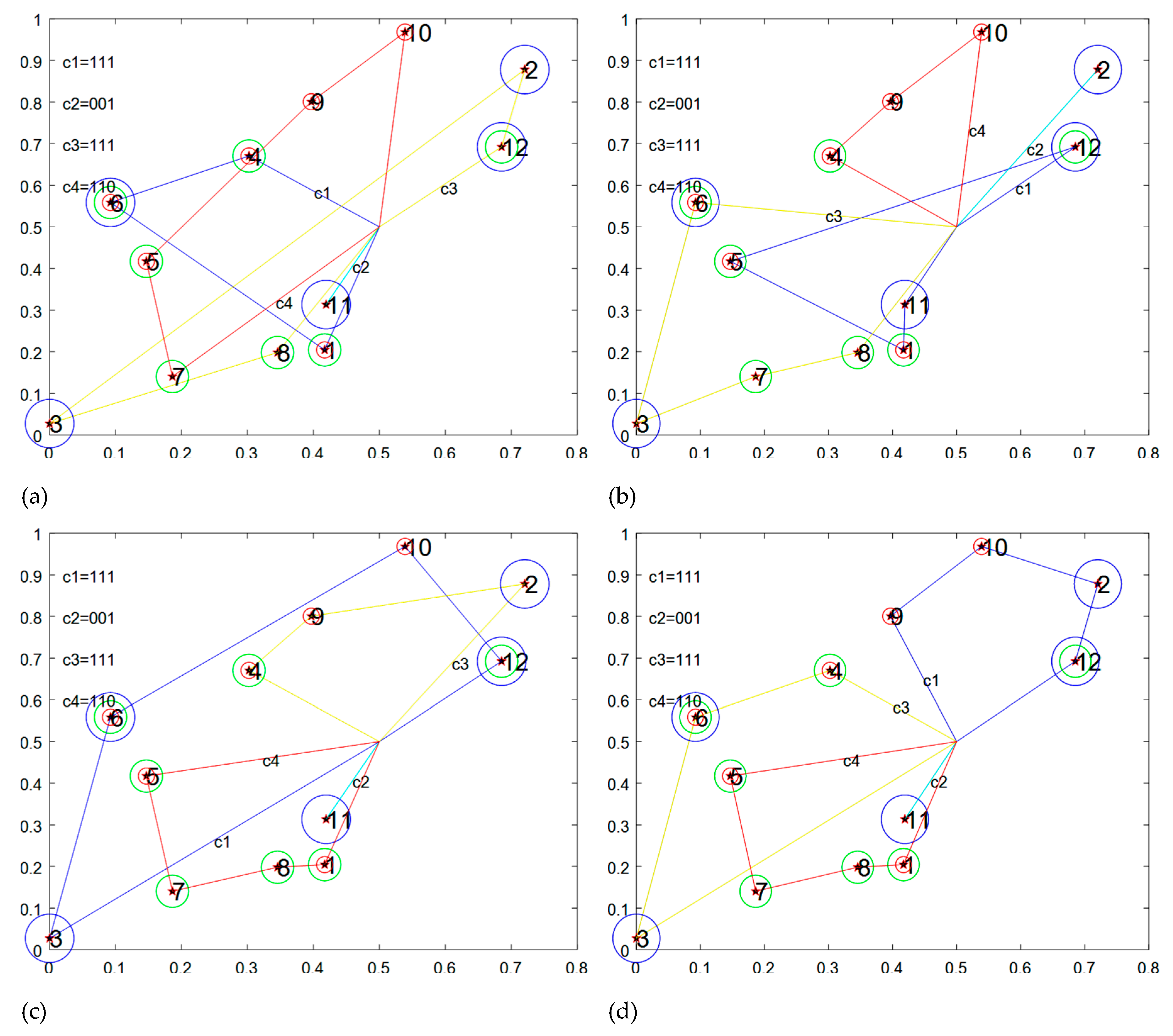
Table 5 and Figure 6 shows the task assignment results. The numbers in the table represent the task sequence numbers. For example, indicates that robot is assigned to tasks , and , and the sorting in the table indicates the order in which the tasks are executed. The programs of the five algorithms were run 10 times each, and the average fitness value, best fitness value, and solution time are shown in Table 6. From the results in Table 6, it can be observed that the t-SDBO algorithm performs better than the other four algorithms, with an average fitness value of 4.3556 and a best fitness value of 4.3213.The results indicate that the proposed algorithm provides better solution quality than the four comparison methods in this scenario. In particular, the improvement over SDBO supports the effectiveness of introducing adaptive t-distribution mutation in addition to Sine-chaotic initialization.
Figure 5.
Visualization of allocation schemes for the four algorithms: (a) PSO. (b) SSA. (c) DBO. (d) t-SDBO.
Figure 5.
Visualization of allocation schemes for the four algorithms: (a) PSO. (b) SSA. (c) DBO. (d) t-SDBO.
In terms of computational cost, t-SDBO requires an average solution time of 3.3069 s, which is higher than that of standard DBO and SDBO but remains comparable to those of PSO and SSA. This result indicates that the improved solution quality is accompanied by additional computational overhead. Therefore, the principal advantage demonstrated by this experiment is the improvement in optimization quality and convergence behavior, rather than a reduction in the absolute solution time.
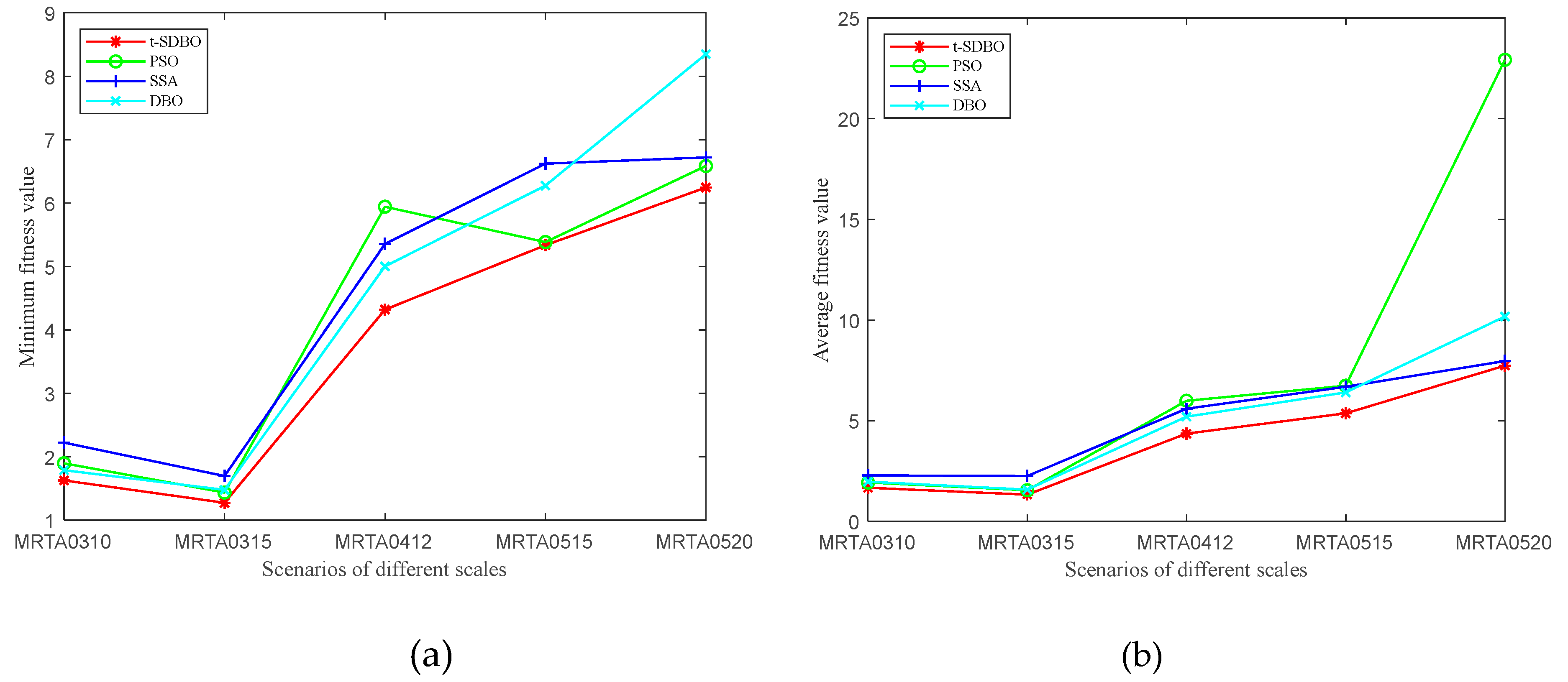
To investigate the performance of the proposed algorithm under different MRTA problem scales, t-SDBO, PSO, SSA, and standard DBO were applied to five scenarios with different numbers of robots and tasks. The experimental scenarios were denoted as MRTA0310, MRTA0315, MRTA0412, MRTA0515, and MRTA0520. For example, MRTA0310 represents a scenario involving three robots and ten tasks.
Each algorithm was independently executed ten times for each scenario, and the minimum and average fitness values were recorded. The comparative results are presented in Figure 6, where Figure 6a shows the minimum fitness values and Figure 6b shows the average fitness values.
Figure 6.
Comparison of different scales of MRTA experiments: (a) Optimal fitness value. (b) Average fitness value.
Figure 6.
Comparison of different scales of MRTA experiments: (a) Optimal fitness value. (b) Average fitness value.
4.2. Experiment 2: ROS/Gazebo Multi-Robot Simulation
To further evaluate the feasibility of the proposed t-SDBO algorithm in a multi-robot system, simulation experiments were conducted using ROS, Gazebo, and RViz. The experimental framework integrates the proposed task allocation module with robot navigation, motion control, mapping, and localization components. In addition to the indoor and outdoor simulation scenarios presented in the original manuscript, a quantitative known-environment benchmark involving five mobile robots and nine navigation tasks was conducted to compare t-SDBO with standard DBO and PSO.
The multi-robot simulation platform was developed under Ubuntu 18.04, ROS Melodic, and Gazebo 9. TurtleBot3 Burger models were used as the mobile robot platforms. For experiments requiring map construction and localization, laser-based Gmapping was employed in the SLAM module, while the ROS multirobot-map-merge package was used for multi-robot map fusion. The task allocation module generated task sequences, and the robots executed the assigned navigation goals through the ROS navigation framework. The overall system architecture is illustrated in Figure 7 [27].
The experiments were designed to examine the integration of task allocation with multi-robot navigation and to provide quantitative evidence of the proposed method’s performance. Since the simulation platform does not fully reproduce differences in physical resources and task execution capabilities, these characteristics were simplified in the known-environment benchmark. Therefore, the quantitative results primarily evaluate allocation and navigation performance under the specified conditions, rather than the complete range of heterogeneous resource constraints considered in the mathematical model.
A multi-robot experimental platform for task allocation in a known environment was constructed based on ROS, Gazebo, and RViz. The experimental environment map was generated using the Gmapping algorithm. The size of the experimental environment was 20 m × 10 m, and the experimental scenario is shown in Figure 8, where the numbers 1-9 represent nine target tasks.
A multi-robot experimental platform for task allocation in a known environment was constructed based on ROS, Gazebo, and RViz. The experimental environment map was generated using the Gmapping algorithm. The size of the experimental environment was 20m×10m, and the experimental scenario is shown in Figure 8, where the numbers 1-9 represent nine target tasks.
The experimental tests were conducted based on the move_base framework. Five mobile robots were assigned tasks using the task allocation algorithm proposed in this chapter. Each robot then navigated to its assigned navigation points (target tasks) using the navigation system provided by the move_base framework. Because the experimental conditions could not represent the resource requirements of robots and target tasks, the nine navigation points were assigned identical resource requirements and value coefficients. Similarly, the five mobile robots were assigned identical resource configurations and capability value coefficients. The initial information of the five mobile robots and nine navigation points is presented in Table 7 and Table 8, respectively.
To evaluate the practical performance of the proposed t-SDBO algorithm in the above experiment, the DBO and PSO algorithms were used for comparison. The navigation point allocation results obtained by the different algorithms are presented in Table 9. The numbers in the table represent navigation point identifiers, and their order indicates the sequence in which the navigation points are visited. For example, <2,3> indicates that mobile robot is assigned navigation points and , and that robot first moves to and then to .
The experimental process of the t-SDBO algorithm is shown in Figure 2.14, which presents five representative time instants. The images in the left column show the positions of the robots in Gazebo as they reach the navigation points at different times. The dark blue, green, red, yellow, and light blue circles represent the positions of robots , , , , and , respectively. The images in the right column show the corresponding robot operating states in RViz. The dark blue, green, red, light blue, and yellow trajectories represent the trajectories of robots , , , , and , respectively.
Figure 9.
Experimental Process of the t-SDBO Algorithm.
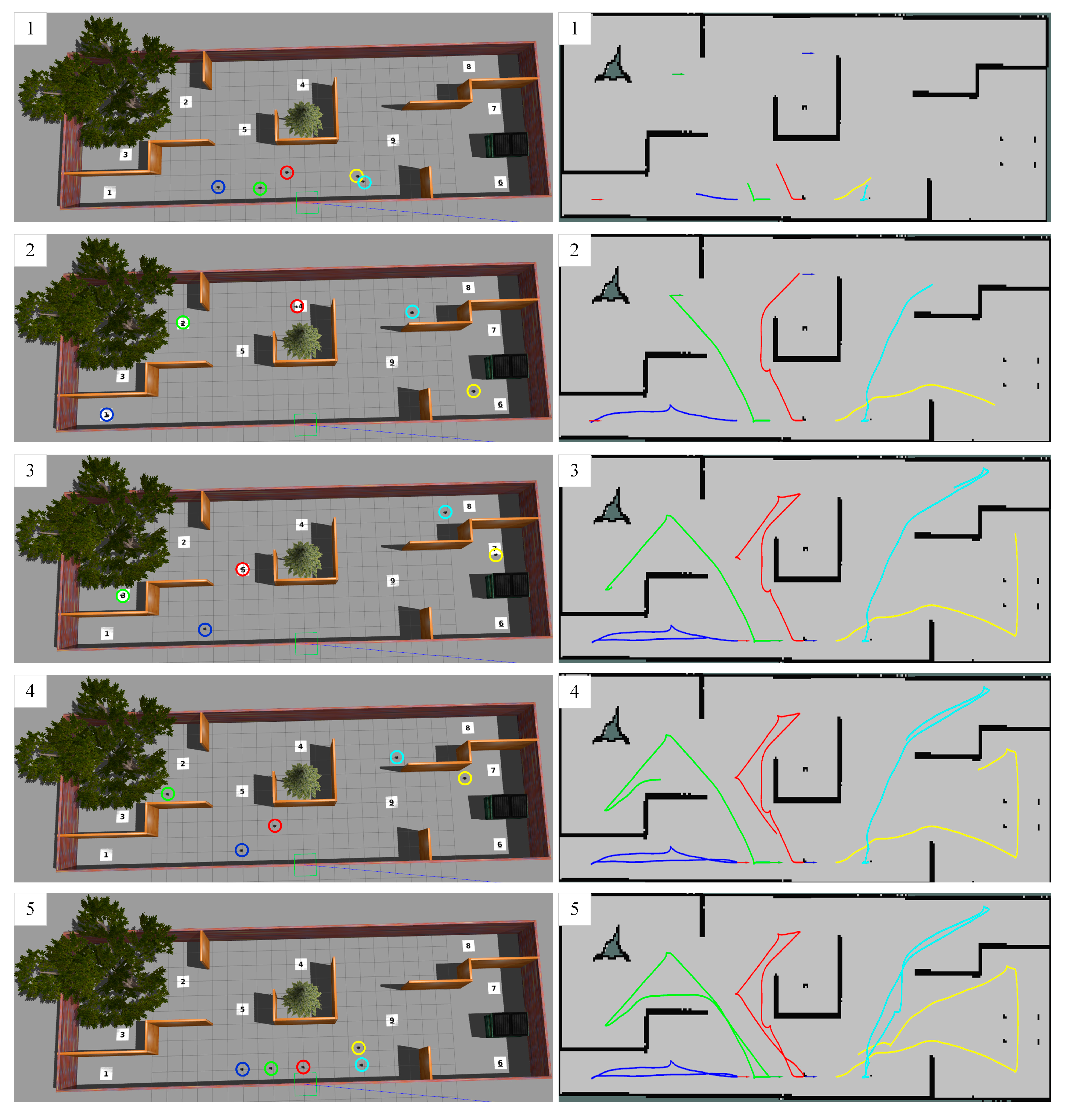
To quantitatively evaluate navigation performance, five experimental trials were conducted for each of the three algorithms: t-SDBO, standard DBO, and PSO. The reported results include total navigation time, total travel distance, average travel distance per robot, and task completion success rate. The original numerical results are presented in Table 10 without modification.
As shown in Table 10, t-SDBO achieves the lowest reported navigation time and travel distance among the three algorithms. Compared with standard DBO, t-SDBO reduces the total navigation time by 5.89s (3.50%) and the total travel distance by 6.04 m (4.72%). The average travel distance per robot decreases from 25.604m to 24.396m, corresponding to the same relative reduction of 4.72%. Both algorithms achieve a reported task completion success rate of 100%, indicating that the improvement in navigation efficiency is obtained without a reduction in the reported completion performance.
Compared with PSO, t-SDBO reduces the total navigation time by 26.83s (14.17%) and the total travel distance by 11.13m (8.36%). The average travel distance decreases from 26.622m to 24.396m, also representing an 8.36% reduction. In addition, the reported success rate increases from 98% to 100%, an improvement of 2 percentage points. These results indicate that the proposed algorithm provides a more efficient allocation scheme in the considered navigation benchmark.
The quantitative results complement the fitness-based comparisons presented in Experiments 1. Whereas the earlier experiments evaluate the optimization performance of t-SDBO using the mathematical objective function, the five-robot benchmark provides additional evidence based on navigation-related measures. The reductions in navigation time and travel distance suggest that improvements in task allocation quality can translate into more efficient multi-robot execution in the simulated environment.
5. Conclusions
This paper proposed t-SDBO, a heterogeneous multi-robot task allocation algorithm integrating Sine-chaotic initialization and adaptive t-distribution mutation. A task allocation model considering time-dependent benefits, travel costs, completion time, and operational constraints was established. The proposed algorithm combines real-valued encoding–decoding, Sine-chaotic initialization, and adaptive mutation with dynamic selection to improve population diversity and alleviate premature convergence.
Comparative experiments demonstrated that t-SDBO achieved an average fitness of 4.3556 and a best fitness of 4.3213 in the four-robot, twelve-task scenario, outperforming the comparison algorithms in solution quality. In the supplementary five-robot navigation benchmark, t-SDBO reduced navigation time by 3.50% and 14.17%, and travel distance by 4.72% and 8.36%, compared with DBO and PSO, respectively, while achieving a reported success rate of 100%. These results support the effectiveness and simulation-level feasibility of the proposed method. Future work will investigate dynamic task allocation and validate the algorithm on physical heterogeneous multi-robot platforms.
Author Contributions
Conceptualization, Y.N. and L.W.; methodology, Y.N., W.Y. and J.Z.; software, Y.N. and W.Y.; validation, Y.N., X.W. and R.A.; formal analysis, Y.N. and J.Z.; investigation, X.W. and K.L.; resources, L.W. and K.L.; data curation, W.Y. and R.A.; writing—original draft preparation, Y.N.; writing—review and editing, Y.N., L.W. and J.Z.; visualization, W.Y. and X.W.; supervision, L.W. and J.Z.; project administration, L.W.; funding acquisition, L.W. All authors have read and agreed to the published version of the manuscript.
Funding
This research received no external funding.
Data Availability Statement
Not applicable.
Acknowledgments
Not applicable.
Conflicts of Interest
The authors declare no conflicts of interest.
Abbreviations
The following abbreviations are used in this manuscript:
| MRS | Multi-Robot System |
| MRTA | Multi-Robot Task Allocation |
| MTSP | Multiple Traveling Salesman Problem |
| DBO | Dung Beetle Optimizer |
| SDBO | Sine-Chaotic Dung Beetle Optimizer |
| t-SDBO | Sine-Chaotic Dung Beetle Optimizer with Adaptive t-Distribution Mutation |
| PSO | Particle Swarm Optimization |
| SSA | Sparrow Search Algorithm |
| ROS | Robot Operating System |
| RViz | ROS Visualization |
| SLAM | Simultaneous Localization and Mapping |
References
- Ning, Y.; Li, T.; Yao, C.; Du, W.; Zhang, Y. HMS-RRT: A novel hybrid multi-strategy rapidly-exploring random tree algorithm for multi-robot collaborative exploration in unknown environments. Expert Syst. With Appl. 2024, 247, 123238. [Google Scholar] [CrossRef]
- Wang, Z.; Tian, G. Hybrid offline and online task planning for service robot using object-level semantic map and probabilistic inference. Inf. Sci. 2022, 593, 78–98. [Google Scholar] [CrossRef]
- Djenadi, A.; Khanouche, M. E.; Mendil, B. A lexicographic optimization-based approach for efficient task allocation in industrial transportation multi-robot systems. Expert Syst. With Appl. 2024, 257, 124998. [Google Scholar] [CrossRef]
- Morim, A.; Campuzano, G.; Amorim, P.; Mes, M.; Lalla-Ruiz, E. The drone-assisted vehicle routing problem with robot stations. Expert Syst. With Appl. 2024, 238, 121741. [Google Scholar] [CrossRef]
- Abujabal, N.; Fareh, R.; Sinan, S.; Baziyad, M.; Bettayeb, M. A comprehensive review of the latest path planning developments for multi-robot formation systems. Robotica 2023, 41(7), 2079–2104. [Google Scholar] [CrossRef]
- Wang, T.; Du, X.; Chen, M.; Li, K. Hierarchical Relational Graph Learning for Autonomous Multirobot Cooperative Navigation in Dynamic Environments. IEEE Trans. Comput.-Aided Des. Integr. Circuits Syst. 2023, 42(11), 3559–3570. [Google Scholar] [CrossRef]
- Wang, F.; Huang, Z.; Han, M.; Xing, L.; Wang, L. A knee point based coevolution multi-objective particle swarm optimization algorithm for heterogeneous UAV cooperative multi-task allocation. Acta Autom. Sin. 2023, 49(2), 399–414. [Google Scholar]
- Quinton, F.; Grand, C.; Lesire, C. Market approaches to the multi-robot task allocation problem: a survey. J. Intell. Robot. Syst. 2023, 107(2), 29. [Google Scholar] [CrossRef]
- Dai, W.; Lu, H.; Xiao, J.; Zeng, Z.; Zheng, Z. Multi-robot dynamic task allocation for exploration and destruction. J. Intell. Robot. Syst. 2020, 98, 455–479. [Google Scholar] [CrossRef]
- Song, W.; Gao, Y.; Shen, L.; Zhang, Y. A multi-robot task allocation algorithm based on near-field subset partition. Robot 2021, 43(5), 629–640. [Google Scholar]
- Alitappeh, R. J.; Jeddisaravi, K. Multi-robot exploration in task allocation problem. Appl. Intell. 2022, 52(2), 2189–2211. [Google Scholar] [CrossRef]
- Martin, J. G.; Frejo, J. R. D.; García, R. A.; Camacho, E. F. Multi-robot task allocation problem with multiple nonlinear criteria using branch and bound and genetic algorithms. Intell. Serv. Robot. 2021, 14(5), 707–727. [Google Scholar] [CrossRef]
- Ghassemi, P.; Chowdhury, S. Multi-robot task allocation in disaster response: Addressing dynamic tasks with deadlines and robots with range and payload constraints. Robot. Auton. Syst. 2022, 147, 103905. [Google Scholar] [CrossRef]
- Zhang, D.; Xie, G.; Yu, J.; Wang, L. Adaptive task assignment for multiple mobile robots via swarm intelligence approach. Robot. Auton. Syst. 2007, 55(7), 572–588. [Google Scholar] [CrossRef]
- Kong, X.; Gao, Y.; Wang, T.; Liu, J.; Xu, W. (2019). Multi-robot task allocation strategy based on particle swarm optimization and greedy algorithm. In 2019 IEEE 8th joint international information technology and artificial intelligence conference, pp. 1643-1646.
- Zhao, H.; Tang, L.; Li, J. R.; Liu, J. Strengthening evolution-based differential evolution with prediction strategy for multimodal optimization and its application in multi-robot task allocation. Appl. Soft Comput. 2023, 139, 110218. [Google Scholar] [CrossRef]
- Feng, B.; Jiang, X.; Li, B.; Zhou, Q.; Bi, Y. An adaptive multi-RRT approach for robot motion planning. Expert Syst. With Appl. 2024, 252, 124281. [Google Scholar] [CrossRef]
- Golmisheh, F. M.; Shamaghdari, S. Distributed safe formation maneuver control of Euler–Lagrange multi-agent systems in a partially unknown environment by safe reinforcement learning. Robot. Auton. Syst. 2023, 167, 104486. [Google Scholar] [CrossRef]
- Xue, J.; Shen, B. Dung beetle optimizer: A new meta-heuristic algorithm for global optimization. J. Supercomput. 2023, 79(7), 7305–7336. [Google Scholar] [CrossRef]
- Chen, S. T.; Ermiş, G.; Sharpanskykh, A. Multi-agent planning and coordination for automated aircraft ground handling. Robot. Auton. Syst. 2023, 167, 104480. [Google Scholar] [CrossRef]
- Zheng, J.; Hong, Y.; Xu, W.; Li, W.; Chen, Y. An effective iterated two-stage heuristic algorithm for the multiple Traveling Salesmen Problem. Comput. Oper. Res. 2022, 143, 105772. [Google Scholar] [CrossRef]
- Han, D.; Jiang, H.; Wang, L.; Zhu, X.; Chen, Y.; Yu, Q. Collaborative Task Allocation and Optimization Solution for Unmanned Aerial Vehicles in Search and Rescue. Drones 2024, 8(4), 138. [Google Scholar] [CrossRef]
- Zhang, C.; Ding, S. A stochastic configuration network based on chaotic sparrow search algorithm. Knowl.-Based Syst. 2021, 220, 106924. [Google Scholar] [CrossRef]
- Zhang, W.; Liu, S. Improved sparrow search algorithm based on adaptive t-distribution and golden sine and its application. Microelectron. Comput. 2022, 39(3), 17–24. [Google Scholar]
- Jain, M.; Saihjpal, V.; Singh, N.; Singh, S. B. An overview of variants and advancements of PSO algorithm. Appl. Sci. 2022, 12(17), 8392. [Google Scholar] [CrossRef]
- Wang, X.; Liu, J.; Hou, T.; Pan, C. The SSA-BP-based potential threat prediction for aerial target considering commander emotion. Def. Technol. 2022, 18(11), 2097–2106. [Google Scholar] [CrossRef]
- Ning, Y.; Li, T.; Yao, C.; Shao, J. Multi-robot Cooperative Space Exploration Method Based on Rapidly-exploring Random Trees and Greedy Frontier-based Exploration. Robot 2022, 44(6), 708–719. [Google Scholar]
Figure 1.
Illustration of task allocation for two heterogeneous robots.
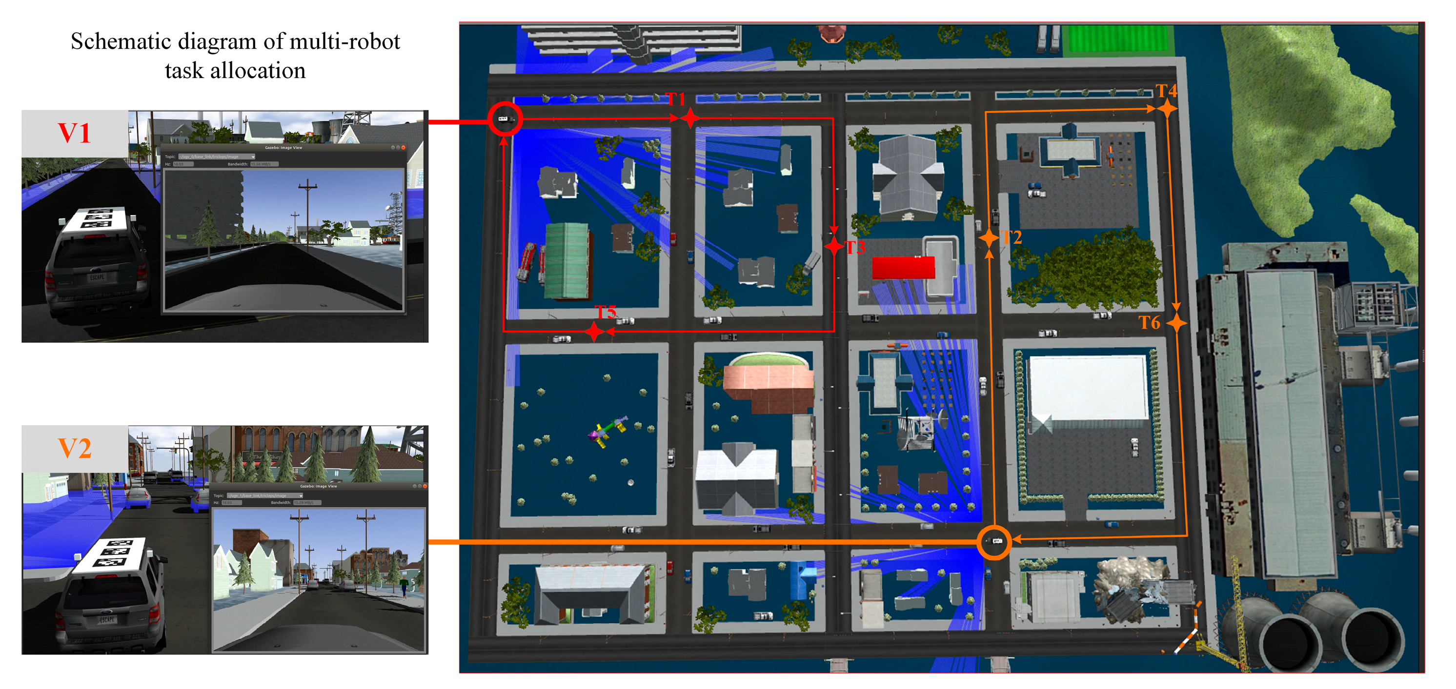
Figure 2.
Schematic diagram of the main process of the algorithm.
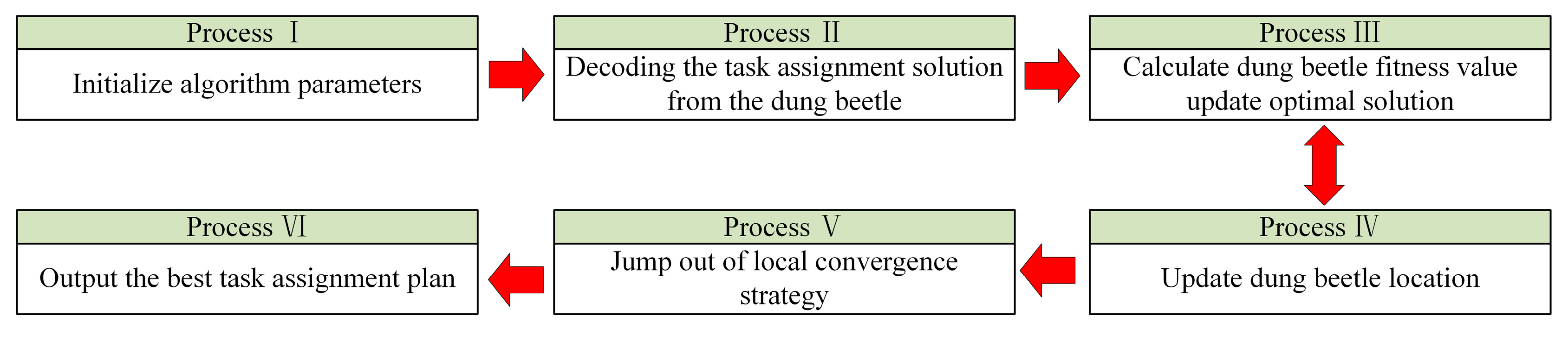
Figure 3.
Schematic diagram of multi-robot task assignment.
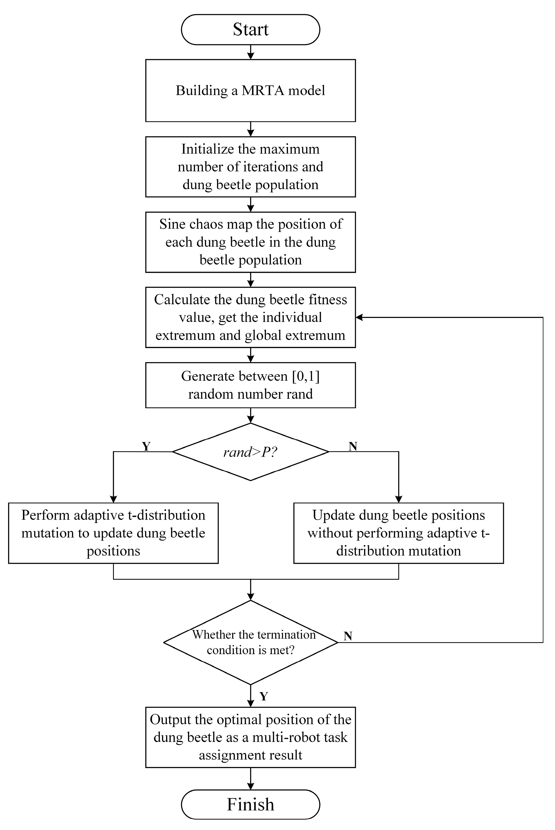
Figure 4.
Schematic diagram of the experimental scene.
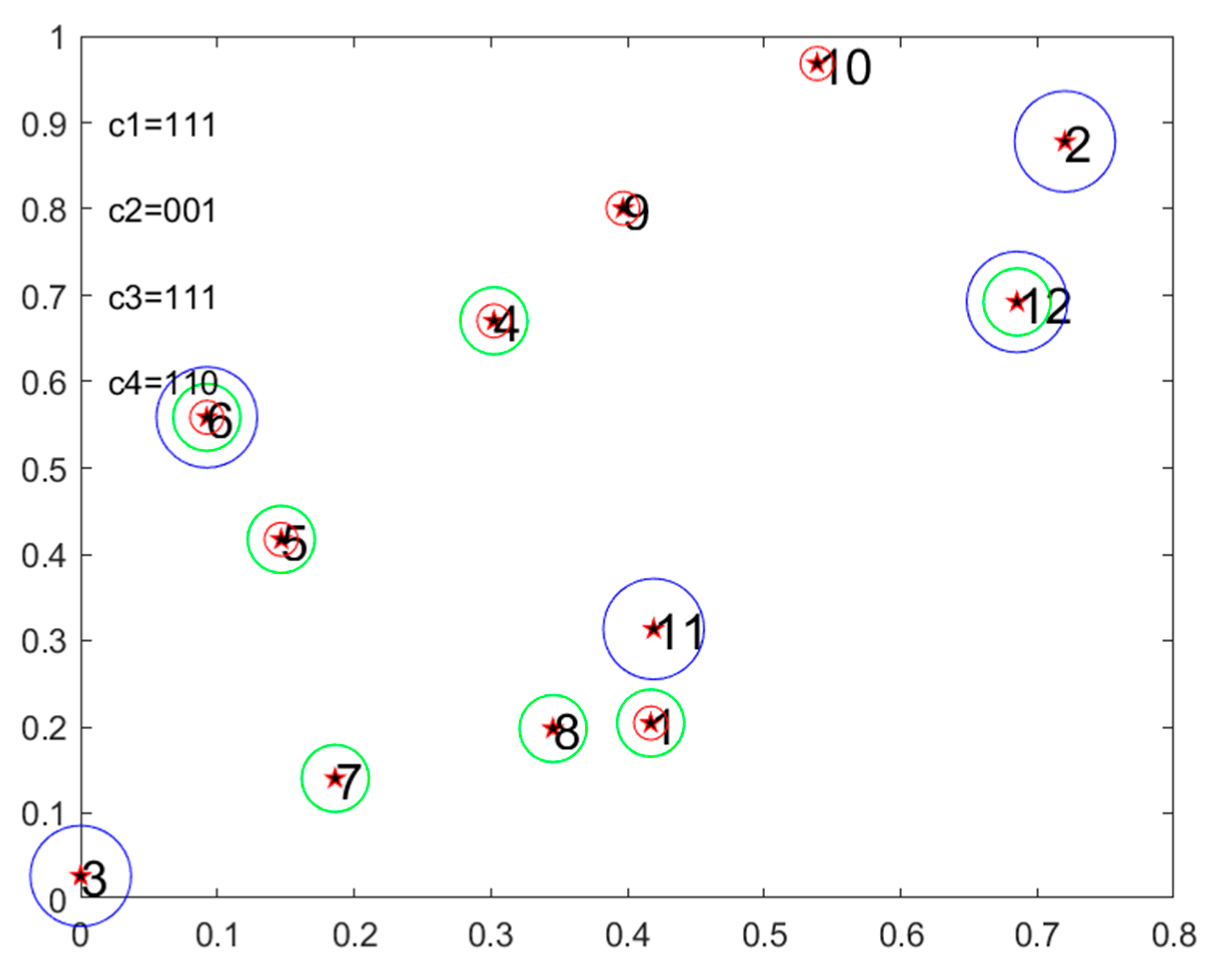
Figure 5.
The graph of fitness value changing with the number of iterations.
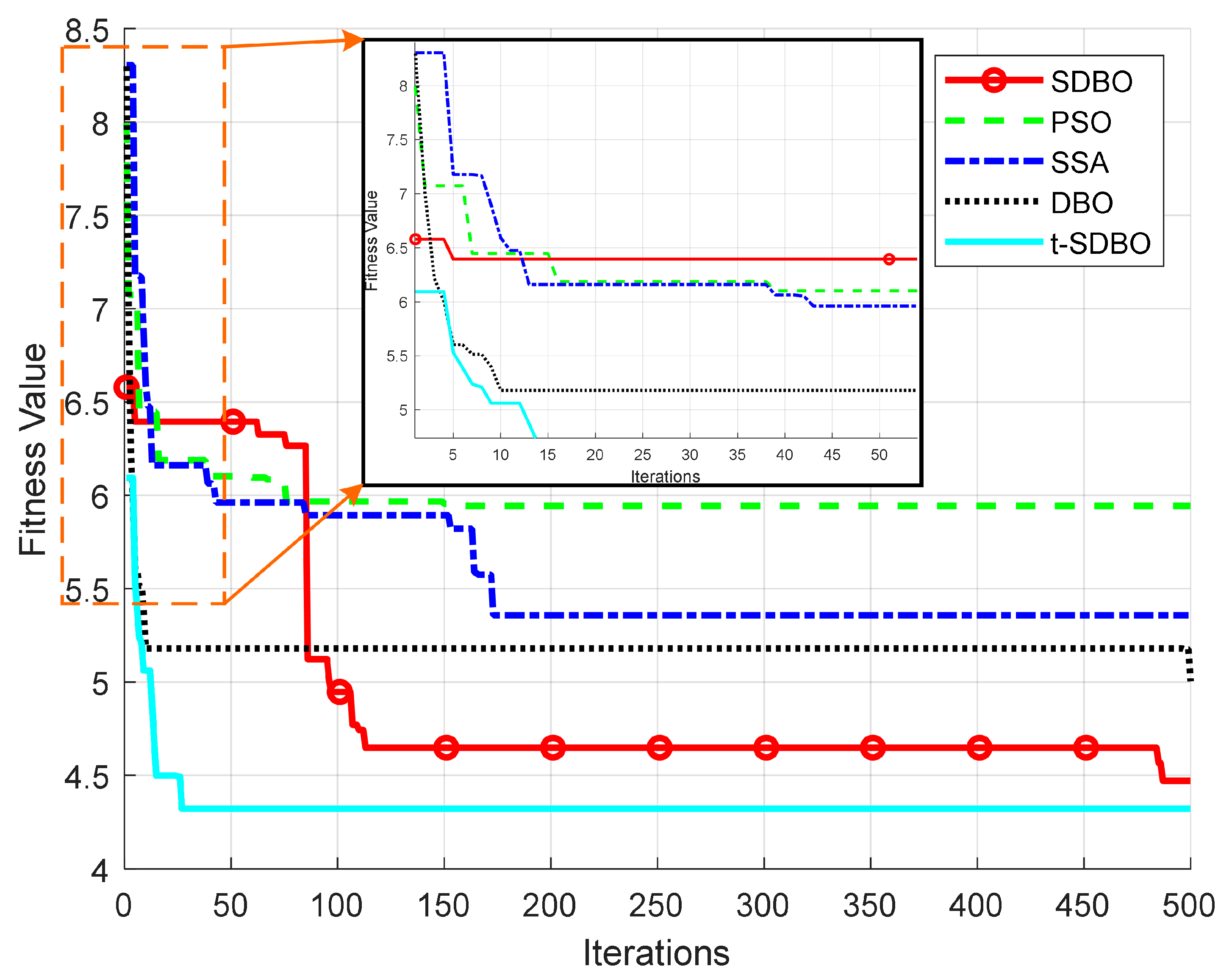
Figure 7.
Frame diagram of multi-robot system.
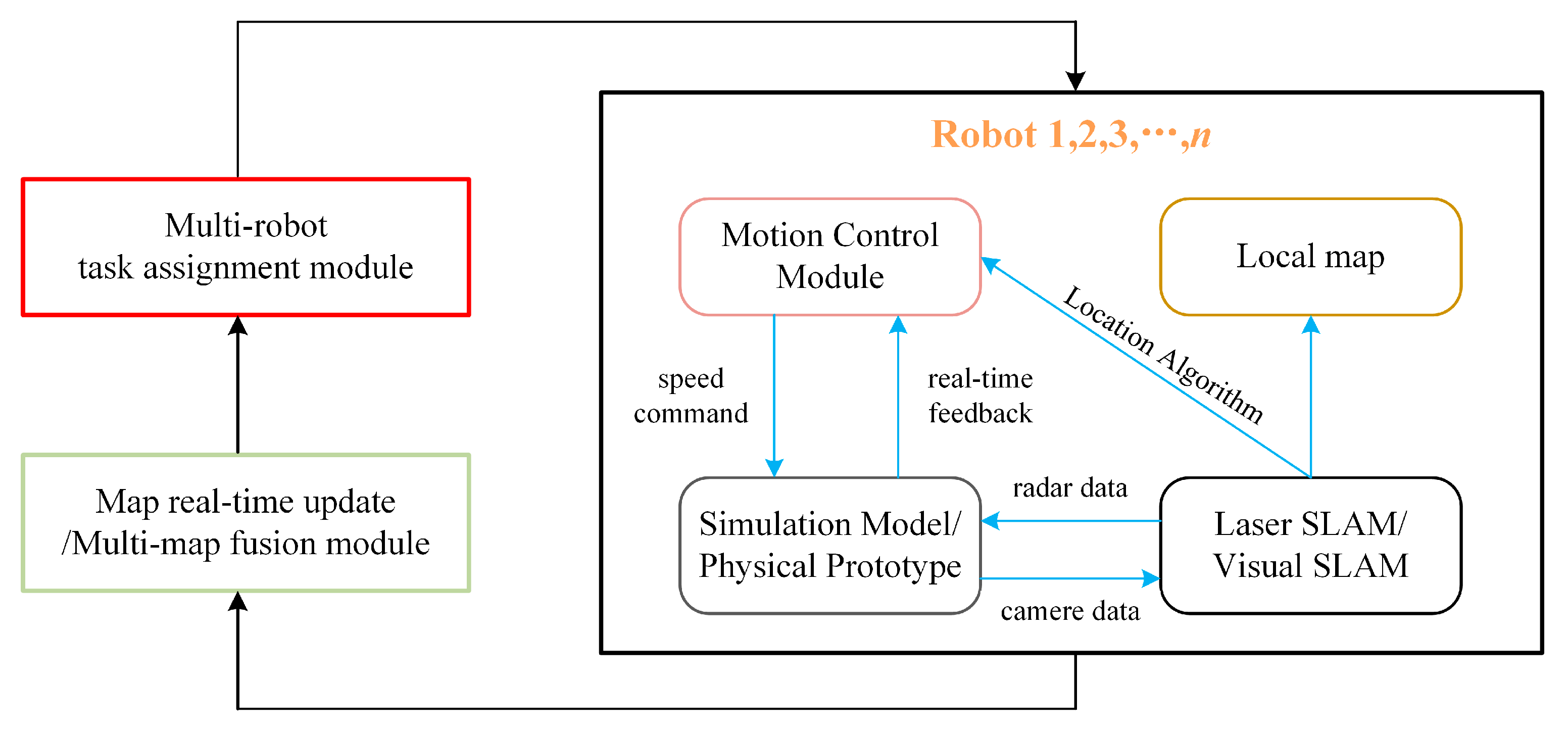
Figure 8.
Experimental simulation environment: (a) Simulation environment in Gazebo. (b) Simulation environment map in RViz.
Figure 8.
Experimental simulation environment: (a) Simulation environment in Gazebo. (b) Simulation environment map in RViz.
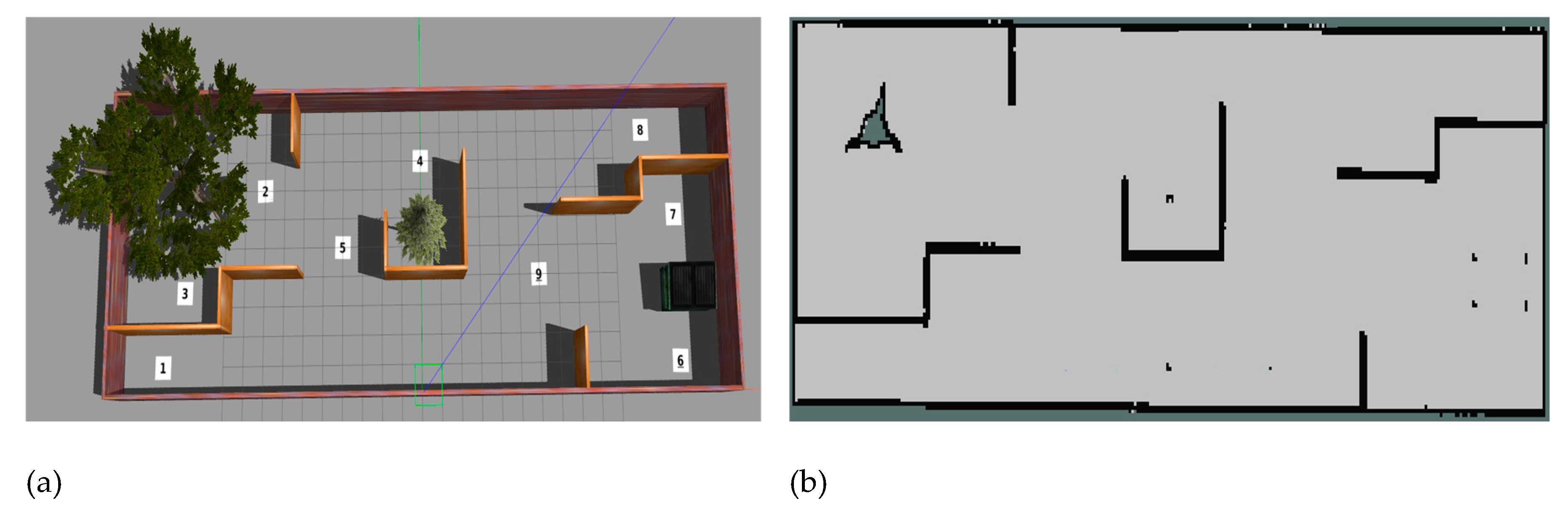

Table 1.
Dung beetle positions and their corresponding assignment results.
| Task | result | |||
|---|---|---|---|---|
| 1.62 | 1 | 0.62 | ||
| 1.67 | 1 | 0.67 | ||
| 2.02 | 2 | 0.02 | ||
| 1.99 | 1 | 0.99 | ||
| 2.55 | 2 | 0.55 | ||
| 2.69 | 2 | 0.69 | ||
| 1.38 | 1 | 0.38 | ||
| 1.08 | 1 | 1.08 |
Table 2.
Task assignment scheme.
| Robot | Execution task sequence number |
|---|---|
Table 3.
Robot initial information.
| Robot | Location | Resource type | Task load |
|---|---|---|---|
| 4 | |||
| 4 | |||
| 4 | |||
| 4 |
Table 4.
Task initial information.
| Task | Location | Resource type | Task time window | Task value |
|---|---|---|---|---|
| (0.42,0.21) | (1,1,0) | (0.27,2.40) | 0.69 | |
| (0.72,0.88) | (0,0,1) | (0.86,9.07) | 0.99 | |
| (0.01,0.03) | (0,0,1) | (0.43,4.98) | 0.17 | |
| (0.30,0.67) | (1,1,0) | (0.96,2.65) | 0.13 | |
| (0.14,0.42) | (1,1,0) | (0.66,10.27) | 0.93 | |
| (0.10,0.56) | (1,1,1) | (0.62,4.48) | 0.70 | |
| (0.19,0.14) | (0,1,0) | (0.12,8.51) | 0.07 | |
| (0.35,0.20) | (0,1,0) | (0.95,8.26) | 0.76 | |
| (0.40,0.80) | (1,0,0) | (0.45,9.83) | 0.76 | |
| (0.54,0.97) | (1,0,0) | (0.58,7.24) | 0.93 | |
| (0.42,0.31) | (0,0,1) | (0.41,8.51) | 0.72 | |
| (0.69,0.69) | (0,1,1) | (0.24,4.49) | 0.13 |
Table 5.
Task assignment results of different algorithms.
| Algorithm | ||||
|---|---|---|---|---|
| SDBO | <12,2,10> | <11> | <9,4,6,3> | <5,7,8,1> |
| PSO | <4,6,1> | <11> | <12,2,3,8> | <7,5,9,10> |
| SSA | <12,5,1,11> | <2> | <6,3,7,8> | <10,9,4> |
| DBO | <3,6,10,12> | <11> | <2,9,4> | <5,7,8,1> |
| t-SDBO | <9,10,2,12> | <11> | <4,6,3> | <5,7,8,1> |
Table 6.
Comparison results of different algorithms.
| Algorithm | Average fitness value | Optimal fitness value | Average solution time/s |
|---|---|---|---|
| SDBO | 4.9544 | 4.4714 | 3.0968 |
| PSO | 5.9945 | 5.9442 | 3.3295 |
| SSA | 5.5911 | 5.3573 | 3.4064 |
| DBO | 5.1971 | 5.0037 | 2.8184 |
| t-SDBO | 4.3556 | 4.3213 | 3.3069 |
Table 7.
Initial Information of the Mobile Robots.
| Robot | Position (m) | Maximum Task Load |
| (-4.0,1.0) | 2 | |
| (-2.0,1.0) | 2 | |
| (0.0,1.0) | 2 | |
| (2.0,1.0) | 2 | |
| (4.0,1.0) | 2 |
Table 8.
Initial Information of the Navigation Points.
| Navigation Point | Position (m) | Time Window (s) |
| (-13.0,1.0) | (0,60) | |
| (-8.0,7.0) | (30,100) | |
| (-12.0,3.5) | (20,120) | |
| (0.0,8.0) | (5,70) | |
| (-4.0,5.0) | (30,120) | |
| (13.0,1.0) | (0,120) | |
| (13.0,6.0) | (30,180) | |
| (11.5,9.0) | (50,150) | |
| (6.0,4.0) | (30,170) |
Table 9.
Navigation Point Allocation Results.
| Algorithm | |||||
| t-SDBO | <1> | <2,3> | <4,5> | <6,7> | <8,9> |
| DBO | <1> | <3,5> | <2,4> | <6,7> | <8,9> |
| PSO | <1,5> | <2,3> | <4> | <6,9> | <7,8> |
Table 10.
Quantitative comparison of navigation performance.
| Algorithm | Total navigation time (s) | Total travel distance (m) | Average travel distance (m) | Success rate |
| t-SDBO | 162.51 | 121.98 | 24.396 | 100% |
| DBO | 168.40 | 128.02 | 25.604 | 100% |
| PSO | 189.34 | 133.11 | 26.622 | 98% |
Disclaimer/Publisher’s Note: The statements, opinions and data contained in all publications are solely those of the individual author(s) and contributor(s) and not of MDPI and/or the editor(s). MDPI and/or the editor(s) disclaim responsibility for any injury to people or property resulting from any ideas, methods, instructions or products referred to in the content. |
© 2026 by the authors. Licensee MDPI, Basel, Switzerland. This article is an open access article distributed under the terms and conditions of the Creative Commons Attribution (CC BY) license (http://creativecommons.org/licenses/by/4.0/).
Copyright: This open access article is published under a Creative Commons CC BY 4.0 license, which permit the free download, distribution, and reuse, provided that the author and preprint are cited in any reuse.