

Submitted:
09 September 2026
Posted:
14 September 2026
You are already at the latest version
Abstract
Memory-dependent evolution equations replace the time derivative of the state with a convolution against a memory kernel \( K(t) \), and appear throughout anomalous diffusion, viscoelasticity, and tumour-growth modelling.\( K \) is usually fixed a priori, most often to the power-law kernel of a Caputo fractional derivative. We investigate the joint recovery of the memory kernel K and the state u using a physics-informed neural network (PINN) trained by a block-coordinate Variable Projection (VarPro) scheme% , and we do so across four structurally different parametrizations: a non-negative Prony series, a fractional (Caputo) power law, a stretched exponential, and a shape-constrained free spline. On a synthetic benchmark the state is recovered with relative\( L^2 \) errors below \( 0.05\% \) across all four families, while kernel recovery varies sharply with the family: \( 0.03\% \) for the single-parameter fractional kernel, a \( 2--4\% \) structural gap for the Prony series that a systematic ablation (mode count, parameter bounds, data volume, optimizer iterations) fails to close, and an intermediate \( 5.7\% \) for the stretched exponential. A local sensitivity (Fisher-information-type) analysis at the exact solution, requiring no training, shows that the persistent instability of the individual Prony parameters is primarily associated with poor parameter identifiability rather than solely with optimization failure: its column-normalized condition number is more than two orders of magnitude worse when the true decay rates sit a factor of \( 4 \)apart than when they are well separated. Remarkably, this parameter-level non-identifiability does not prevent accurate recovery of the aggregated kernel function \( K(t) \) itself. For the stretched-exponential kernel, the initial instability was traced to a regularization term inherited from the Prony formulation. Removing this term reduced the kernel error from 13% to 5.7%. We further test and reject the classical hypothesis that a wider observation window would close the remaining gap. A shape-constrained spline that assumes only positivity, monotonicity, and convexity, with no exponential or power-law structure at all, recovers the benchmark kernel's shape to within \( 6\% \), matching the correctly specified parametric families and showing that the difficulty above sits in each family's own parametrization rather than in the learning problem itself. Finally, a Gauss--Newton/Laplace uncertainty analysis and an \( 8 \)-replicate nonlinear training ensemble converge on the same conclusion: even in the badly conditioned Prony case, individual rates carry uncertainty of hundreds to millions of percent, while the aggregated function \( K(t) \) stays determined to within a few percent, a quantitative instance of the classical inverse-problem distinction between parameter- and function-level identifiability. Overall, accurate state recovery is shown, both empirically and analytically, not to guarantee a uniquely recoverable memory operator.
Keywords:
physics-informed neural networks
; memory kernels
; inverse problems
; identifiability
; Volterra operators
; fractional differential equations
MSC: 35R30; 45D05; 45Q05; 26A33; 65N21; 68T05
1. Introduction
Memory effects appear in anomalous diffusion, viscoelasticity, tumour growth [1], and many other multiscale phenomena, and are typically modelled by replacing an integer-order time derivative with a fractional (Caputo) one [2],
which assumes a specific power-law kernel a priori. Physics-informed neural networks (PINNs) [3] embed the governing PDE into the training loss of a neural network approximating the state; fractional PINNs (fPINNs) [4] extend this to fractional-order problems, but still assume the fractional order — and hence the kernel — is known in advance. Closer to our setting, recent PINN-based inverse frameworks infer the fractional order itself from data in anomalous diffusion and viscoelastic rheology [5], but do not address whether the underlying kernel family is itself identifiable, which is the question this work takes up directly. More broadly, PINN training is known to admit failure modes in which a near-zero residual coexists with an inaccurate solution [6], a phenomenon closely related to, though distinct from, the kernel-state compensation mechanism documented in Section 4.3. Hard-constrained architectures that build initial and boundary conditions directly into the network [7], and rigorous generalization-error estimates for PINN-based inverse problems [8], provide some of the theoretical grounding this work builds on, though neither addresses the parameter-versus-function identifiability distinction studied here; broader reviews of physics-informed machine learning [9] similarly do not treat this distinction directly.
The present problem also belongs to the broader class of inverse operator-identification problems, in which the available observations constrain an unknown constitutive or memory law only through its action on the observed state. This distinction is important: accurate reconstruction of the state does not necessarily imply that the parameters defining the underlying operator are uniquely determined. Similar issues arise in inverse Volterra problems, most classically in kernel identification for viscoelasticity and heat conduction with memory [10], in the general theory of regularization for ill-posed inverse problems [11], in structural and practical identifiability analysis for nonlinear dynamical models [12], and in the sloppy-parameter phenomenon documented across systems biology and other nonlinear models [13], where distinct parameter vectors may produce nearly indistinguishable observable responses.
We consider the inverse problem of learning the memory law jointly with the state while enforcing the governing PDE as a physical constraint. We study this question for the general convolutional evolution equation
of which the fractional (Caputo) derivative is recovered as the special case above. We build a PINN framework that jointly approximates the state u and a general memory operator K, and we investigate the practical identifiability of K: does an accurate state imply a reliable kernel? Rather than fixing a single parametrization for K, we deliberately test the same architecture, loss, and training strategy against four structurally different kernel families: a non-negative Prony series, a fractional (Caputo) power law, a stretched exponential, and a shape-constrained free spline. This common experimental setting allows the effect of kernel parametrization on identifiability to be assessed independently of changes in the state architecture, loss formulation, or training strategy. We find, both empirically and through a rigorous local sensitivity analysis, that an accurate state does not in general imply an accurate kernel, and that the severity of this gap varies sharply across families.
The main contributions of this work are fourfold. First, we formulate a unified physics-informed framework for joint state and memory-kernel reconstruction across several structurally distinct kernel families. Second, we show that state accuracy, kernel-function accuracy, and parameter identifiability constitute distinct levels of the inverse problem. Third, we quantify parameter identifiability independently of neural-network training through local sensitivity and uncertainty analyses. Finally, we demonstrate that increasing the diversity of temporal excitations improves kernel-function identifiability more effectively than simply increasing the number of observations along a single trajectory.
2. Method
2.1. State Network: Hard-Constrained Architecture
The state is represented as
where is a plain multilayer perceptron (5 layers, 128 units, tanh activations). By construction, (2) satisfies and exactly, for any , removing two competing loss terms from the optimization.
2.2. Kernel Network: Non-Negative Prony Series
The memory kernel is parametrized as a Prony series
which is positive, strictly decreasing, and convex by construction for any admissible , with no extra penalty needed to enforce these physical properties. The weights are solved by non-negative least squares (NNLS) [14], which enforces structurally; the rates are mapped through a softplus and clamped to , with .
2.3. Loss Function
Writing the PDE residual as
the training loss is
with . No IC/BC loss term is needed, since these are satisfied exactly by (2). The convolution in R is discretized by Gauss–Legendre quadrature after the substitution , which handles cleanly, on a collocation grid that is quadratically spaced in t (denser near , where the memory kernel varies most rapidly). These hyperparameters, together with the 5-layer, 128-unit architecture, the collocation grid, and the 50-node quadrature used throughout this paper, were selected in preliminary experiments to provide stable state reconstruction and were subsequently kept fixed across kernel families. They are therefore not claimed to be globally optimal; their role is to define a common computational setting in which differences in reconstruction performance can be attributed primarily to the kernel parametrization.
2.4. Training: Block-Coordinate Variable Projection
Since is linear in the weights for fixed rates , we exploit a Variable Projection (VarPro) scheme [15]:
- fix , solve for by NNLS with a column-scaled Tikhonov ridge,
- fix , refine by Adam followed by a short L-BFGS polish on ;
- fix , refine by Adam (a single optimizer instance, persistent across all rounds, driven by a cosine annealing learning-rate schedule) followed by L-BFGS.
The final training procedure includes two additional components: (i) a data-only warm-up of 3000 epochs before the first kernel update, and (ii) a final prune-and-refit step in which modes with negligible weights are removed and the remaining weights are recomputed. The column-scaled ridge in step 1 is itself a deliberate departure from a plain penalty: fast-decaying modes produce small-norm columns in , so a flat ridge barely constrains them. In preliminary experiments, the unscaled penalty provided insufficient regularization of these modes and resulted in excessively large weights. The full loop is repeated for several rounds with early stopping, followed by kernel-only polishing rounds, pruning, and a final state fine-tuning pass.
2.5. Generalizing the Training Scheme to Other Kernel Families
The state network, loss (4), discretization, data-only warm-up, and persistent-optimizer/cosine-annealing schedule are all kernel-agnostic and are reused unchanged for every family below; only the “kernel step” of the VarPro loop differs, according to how much linear structure each family admits.
- Stretched exponential, : a single mode, so the same VarPro pattern as Prony applies with . The amplitude is solved by (unregularized) NNLS given , which are then refined by Adam followed by L-BFGS. Unlike Prony, the column-scaled Tikhonov ridge is not applied here: with only one mode there is no redundant-column risk to guard against, and retaining the Prony-tuned ridge was found to bias A downward by and, through the real correlation between A, , and (Section 5.4), to destabilize the whole alternation. Removing it was necessary to obtain a monotonically decreasing training loss.
- Oscillatory, : the same single-mode VarPro pattern, but A is solved by signed least squares rather than NNLS, since an oscillatory kernel legitimately changes sign.
- Fractional (Caputo), : a single nonlinear parameter with a genuine integrable singularity at . The convolution is discretized with Gauss–Jacobi quadrature (weight after ) rather than Gauss–Legendre; since the Jacobi nodes/weights depend on and are not differentiable through automatic differentiation, is refined by a bounded one-dimensional search (a coarse grid followed by a local scalar minimization) rather than by the gradient-based refinement used for the other kernel families.
For every family, the collocation grid, quadrature order, warm-up, and optimizer schedule of Section 3 are held fixed, so that differences in kernel-recovery accuracy can be attributed to the kernel’s own parametrization rather than to incidental changes in the rest of the pipeline.
3. Synthetic Benchmark
We consider and
the same for every kernel family tested, so that only K and the resulting forcing change across experiments. The network observes only 120 sparse, noise-free samples of u; the kernel is inferred purely through the PDE residual, never directly. Discretization uses a collocation grid (t quadratically spaced), 50 Gauss–Legendre quadrature nodes (or Gauss–Jacobi, for the fractional family), and Prony modes with where applicable.
3.1. Ground-Truth Kernels
Writing (so ), the memory term is with . Three ground truths have been used so far:
- Prony, , : admits an exact closed-form expression as a sum of exponential terms in t.
-
Fractional, : coincides with the Caputo derivative , which, for the polynomial g considered here, has the closed-form expressionThis expression was verified numerically against scipy.integrate.quad, with agreement to approximately .
- Stretched exponential, , , : is evaluated numerically using scipy.integrate.quad, providing an independent high-accuracy reference for the subsequent reconstruction.
An oscillatory ground truth (, , ) has been implemented with the same numerical-quadrature strategy but end-to-end training results for it are still pending at the time of writing (see Section 10).
4. Results
4.1. State Recovery
The trained state achieves relative errors of on the full space–time grid and on the cross-section (final loss , with and ). Comparable state accuracy is also obtained under poorly conditioned kernel parametrizations (see Section 4.3), indicating that state accuracy alone is not sufficient to assess kernel recovery.
4.2. Discrepancy Between State and Kernel Recovery
Figure 1 shows the recovered kernel and state cross-section for the best configuration found. The relative error of the reconstructed kernel over is , compared with for the state.
The learned rates for this run,
reveal the nature of the residual error: one rate lands almost exactly on a true one ( vs. ), but seven of the twelve modes collapse into a cluster near ( each). The cluster should therefore be interpreted as an effective representation of the two low-frequency modes and , rather than as evidence for seven distinct decay scales. Two further modes remain pinned at with non-negligible weight ( each), a residual fast-mode artefact concentrated near . The NNLS residual is essentially flat across polishing rounds (), indicating the fit has actually converged to this configuration rather than merely being under-trained.
4.3. Effect of Regularization and State Pretraining
An earlier version of the pipeline, differing only in the kernel’s regularization and the absence of the data-only warm-up, produced a badly conditioned fit: the learned kernel diverged to values of order 150–175 against a true kernel of order 1–2 (relative error ), while the state itself was also poorly recovered ( error) despite an almost vanishing PDE residual. Figure 2 contrasts this run against the final one, using the identical architecture, benchmark, and governing equation.
This behaviour is consistent with an ill-conditioned inverse problem in which the residual can be driven to near zero by compensating kernel errors against state errors, rather than by recovering either correctly: with 12 free modes and wide rate bounds, the kernel had enough freedom to absorb the PDE residual regardless of whether the state was accurate, leaving the sparse data term with insufficient relative weight to pull the state toward the truth. Two changes resolved this: (i) a data-only warm-up phase, so the state is already a reasonable fit to the data before the kernel is ever touched, and (ii) replacing the flat Tikhonov ridge on the kernel weights with a column-scaled one, which prevents fast-decaying modes (whose basis columns are small in norm) from being assigned unphysically large weights.
4.4. Ablation Study of the Residual Kernel Error
Having fixed the gross pathology above, we then attempted, over several further iterations, to close the remaining – kernel error by tuning the number of modes M, the rate bound , the data volume , and the number of rate-refinement iterations. Table 1 summarizes the outcomes.
None of these changes separated from ; the learned cluster’s effective rate merely drifted between runs (from to to across different configurations), never approaching either true value. Widening in particular let the spurious fast mode drift to an even more extreme rate with a larger weight, worsening the overshoot rather than resolving it. Increasing therefore aggravates the existing parameter degeneracy rather than improving recovery of the true rates. The persistence of the reconstruction error across these ablations suggests that further optimization alone is unlikely to resolve the observed mode degeneracy, and motivated the analytical investigation of Section 5.
4.5. Training-Independent Inverse Reconstruction
The local sensitivity analysis of Section 5 establishes that the Prony parametrization is poorly conditioned at the exact solution. To determine whether the observed mode merging originates from the joint PINN optimization or from the underlying inverse problem, we repeat the reconstruction using the exact state and its exact time derivative, with the neural state network removed entirely. The target is the exact convolution , evaluated by high-accuracy adaptive quadrature independent of the model’s own discretization (to avoid an inverse crime), at the same 40-point, quadratically spaced collocation grid used throughout this work. The kernel is then fit directly against ,
using the same modes, the same bounds, and the same Gauss–Legendre discretization (50 nodes) as the physics-informed experiments, so that only the presence or absence of the neural network and its training dynamics differs. We compare three training-free solvers: (i) the same block-coordinate VarPro scheme as Section 2, with the column-scaled ridge () carried over unchanged, applied directly to instead of to the PINN’s residual; (ii) the identical VarPro scheme with the ridge switched off (), to isolate its effect now that training stability is no longer a concern; and (iii) a fully joint, bounded Levenberg–Marquardt fit (trust-region-reflective least squares) over simultaneously, with no VarPro structure and no ridge at all. Each solver is run from 6 random log-uniform initializations of , and we report the best-converged run, in line with the reporting convention used for Figure 1. Because Prony modes carry no fixed identity, we quantify parameter recovery with a matching-based metric: the 3 highest-weight learned modes are paired with the 3 true modes by optimal (Hungarian) assignment on the column-normalized distance, and we report the resulting relative error.
With the exact state supplied, all three training-free solvers achieve substantially smaller kernel errors than the joint PINN–VarPro pipeline: the bounded Levenberg–Marquardt fit drives the kernel error down to , machine precision for this discretization, and even the ridge-carrying VarPro variant reaches , two orders of magnitude better than PINN–VarPro’s . This confirms that the neural approximation and its training schedule are not what caps the achievable kernel accuracy; a sufficiently well-optimized direct fit recovers almost exactly regardless of solver.
The ridge ablation shows that the column-scaled Tikhonov term, while useful for stabilizing the joint PINN training of Section 4.3, degrades parameter recovery in the exact-state inverse problem. Removing the ridge reduces the kernel error from to and the parameter error from to : freed from the ridge’s pull toward spreading weight across many modes, NNLS’s own preference for sparse solutions lets several seeds converge close to the true 3-mode structure directly, with only a small residual weight left on spurious low-amplitude modes. This does not contradict the local sensitivity analysis of Section 5 (the column-normalized condition number at the true parameters is unchanged by which solver is used), but the particular parameter configuration selected within the degenerate solution set therefore depends strongly on the regularization and optimization strategy, which were tuned for a different purpose (PINN training stability) and were never optimized for parameter recovery in the first place.
Individual parameter recovery still remains imperfect in every training-free configuration (parameter error 9–) despite near-machine-precision function fits, confirming that the parameter-level non-identifiability documented throughout this paper is a property of the Prony inverse problem itself and not an artefact of PINN training. Its specific character, however, is not fixed. The joint PINN pipeline produces mode merging (seven modes collapsing onto a single effective rate near , roughly halfway between the two true rates it conflates); the ridge-carrying exact-state VarPro produces a milder version of the same merging pattern; and the unconstrained Levenberg–Marquardt fit instead produces mode splitting: six near-duplicate copies clustering tightly around , three around , and two around , each cluster’s summed weight closely tracking the corresponding true weight (, , ). Both mode merging and mode splitting are consistent with weak parameter identifiability in the over-parametrized Prony representation. For and a three-mode ground truth, the nine redundant modes introduce non-unique parameter representations of essentially the same kernel function, and whether that non-uniqueness manifests as fusing distinct rates together or as duplicating a single rate several times depends on the solver’s implicit bias (regularized alternation versus unconstrained joint descent) rather than on the inverse problem’s intrinsic geometry, which is identical across all four rows of Table 2. What does not depend on solver choice is the conclusion itself: a near-vanishing residual is compatible with a wide range of internally inconsistent parameter configurations, all of which reconstruct correctly. These training-free results provide additional evidence for the distinction between parameter-level and function-level identifiability discussed in Section 6, obtained here without training any neural network at all, and suggest a concrete practical recommendation: if parameter recovery (rather than kernel recovery) is the goal, the regularization used to stabilize PINN training should not be assumed optimal, and an unregularized, sparsity-promoting refit at convergence may recover the underlying structure considerably better.
4.6. Fractional Kernel Recovery: A Well-Conditioned Single Parameter
Repeating the entire pipeline unchanged except for the kernel family (Section 2.5), with the fractional ground truth of Section 3 (, model initialized at ), produces substantially smaller reconstruction errors: the kernel is recovered to relative error, essentially exact, matching the singular shape and the power-law tail alike (state error on both metrics). Unlike the Prony case, the training loss decreased monotonically and the kernel-only “polishing” rounds converged to a fixed point immediately, with no drift.
This is consistent with the family having only a single free parameter: there is no second rate for to be confused with, so none of the compensation mechanisms responsible for the Prony gap can arise. We return to this contrast quantitatively in Section 5.4.
4.7. Stretched-Exponential Kernel Recovery
The stretched-exponential family, , was tested against its own ground truth (), initialized away from the truth at . Three configurations were tried, summarized in Table 3.
The first configuration reused, unchanged, the column-scaled Tikhonov ridge developed for the Prony family’s redundant-mode problem (Section 4.3). With a single mode there is no redundancy for that ridge to guard against, and it instead measurably biased the amplitude A downward; because A, , and are truly correlated (Section 5.4), this bias propagated into and and appears to have destabilized the block-coordinate alternation, whose training loss increased over the later rounds rather than converging. Adding a multi-start grid search over before local refinement (to rule out a poor initial basin) improved the fit but did not resolve the instability by itself. Removing the Tikhonov term yields a monotonically decreasing training loss and reduces the kernel error to .
Even after both fixes, a real kernel error remains, well above the fractional family’s but well below the Prony family’s near-total mode collapse. Section 5.4 tests whether the remaining discrepancy can be explained by the classical – compensation mechanism reported for Kohlrausch–Williams–Watts relaxation [16].
4.8. Shape-Constrained Free Kernel: Recovering the Shape Without the Functional Form
Every family above assumes a specific functional form (exponentials, a power law, a stretched exponential) and asks whether its own parameters can be recovered. A different question is whether a kernel’s shape can be recovered by a family that assumes nothing about the functional form at all, only two qualitative physical properties: should be positive, monotone decreasing, and convex, as is standard for physically admissible relaxation kernels, without committing to any particular parametric family.
We built from knots via a piecewise-linear spline, guaranteed convex, monotone decreasing, and positive by construction rather than by penalty. Writing the per-segment slopes as (parametrized through a positive final slope magnitude and non-negative gaps, so that non-decreasing, non-positive slopes, the discrete condition for a convex, decreasing piecewise-linear function, hold for any choice of the underlying free parameters, verified numerically before being implemented) and applying a single softplus to the whole interpolated curve at the end (softplus is convex and non-decreasing everywhere, and composing a convex non-decreasing outer function with a convex inner one is itself convex, so positivity is added without breaking either other property), the resulting family has no linear substructure to exploit and is trained jointly with the state network, like the neural kernel, with a longer final fine-tuning budget to compensate for the lack of a dedicated per-round kernel solve.
An initial version with uniformly spaced knots recovered the correct qualitative shape but with a systematic overshoot near and undershoot at larger t (kernel error even after a long training budget). The error is concentrated near , where the curvature of the true kernel is largest and the uniform knot distribution provides the lowest effective resolution. Spacing the knots quadratically instead, denser near (the same reasoning already used for the collocation grid, Section 3), and re-deriving the slope-based construction to preserve convexity under non-uniform spacing (which the original, knot-value-based construction only guaranteed for uniform spacing), reduced the error to (Figure 3), matching the Prony series’ own accuracy on its own benchmark despite assuming no exponential structure whatsoever.
The spline result supports the interpretation that reconstruction difficulty depends strongly on parametrization. Despite making no assumption of exponential structure, the shape-constrained spline achieves a kernel error comparable to that of the correctly specified parametric representation, and considerably better than an over-parametrized version of that same correct family exploring a degenerate manifold (Prony with redundant modes).
4.9. Comparing Kernel Families
Table 4 collects the results above alongside the local-sensitivity condition numbers computed at the true parameters (Section 5 and Section 5.4). Kernel-recovery difficulty spans more than two orders of magnitude across families sharing the same state network, loss, and training strategy, and tracks the condition number of the underlying parameter-to-observation map reasonably well for Prony and fractional – though, as discussed below, not in every detail for the stretched exponential. The shape-constrained spline has no analogous “true parameters” at which to evaluate a condition number, but its error places it in the same regime as the correctly specified parametric families, not as an outlier.
4.10. Local Identifiability of Memory-Operator Parametrizations
The numerical experiments presented in the previous section suggest that accurate state recovery does not necessarily imply accurate recovery of the underlying memory kernel. These results motivate a local identifiability analysis of the kernel parametrization through the sensitivity of the parameter-to-observation map.
Let
denote the memory operator.
Kernel identification consists of solving the nonlinear inverse problem
where the observed quantity g is obtained from the governing PDE.
Since the memory operator is a Volterra convolution, it acts as a smoothing operator, attenuating high-frequency information of the kernel. Consequently, different kernels may produce nearly indistinguishable observations whenever the corresponding Fréchet derivative becomes nearly rank deficient.
5. Local Identifiability Analysis
To test the identifiability-floor hypothesis directly, independently of any neural-network training, optimizer choice, or data sparsity, we carry out a local sensitivity analysis at the exact solution.
5.1. Setup
The discretized memory operator predicts, at each collocation point,
where is built from the same Gauss–Legendre discretization as in training, but using the exact in place of a network’s derivative — removing PINN approximation error entirely from the analysis. We compute the Jacobian J of with respect to the parameters at the true values, for two cases: (a) the benchmark’s actual rates, , and (b) a well-separated control case, , both evaluated at so the comparison is not confounded by redundant modes. Because and live on different scales, we report the condition number of the column-normalized Jacobian, which isolates the geometric (unit-free) conditioning of the problem from an arbitrary parametrization choice.
Proposition 1
(Local amplification of observational perturbations). Let
be the parameter-to-observation map and let
denote its Jacobian at . Assume that has full column rank and smallest singular value .
For sufficiently small perturbations,
Hence, to first order,
and therefore
Thus, perturbations aligned with the least-sensitive singular direction may be amplified by a factor proportional to .
This result is local: it characterizes perturbation amplification in a neighbourhood of and does not imply global non-uniqueness of the inverse problem.
5.2. Results
The condition number is worse for the closely spaced rates than for the separated ones, and every pairwise cosine similarity between rate-sensitivity directions is higher in the close case. This training-independent calculation shows that the close-rate configuration is substantially more ill-conditioned than the well-separated control case: the residual kernel error documented in Table 1 is not an artefact of the optimizer or of data volume, since at the true parameter values themselves, two rates only apart are close to indistinguishable through this residual.
The separated configuration remains moderately ill-conditioned (), consistent with the smoothing character of the underlying convolution-deconvolution problem. Mode separation substantially improves conditioning but does not eliminate the underlying difficulty of the inverse problem.
5.3. Identifiability as a Function of Mode Separation
The comparison above considers only two representative rate configurations. To determine whether the observed conditioning difference reflects a systematic transition rather than a case-specific effect, we next vary the separation between consecutive Prony rates continuously. We consider the three-mode family
with fixed positive weights , and evaluate the column-normalized Jacobian at these parameter values for
This family keeps the relative spacing between consecutive rates fixed at r (each rate is the previous one) while sweeping from nearly coincident () to well separated (), using the identical methodology as Table 5: the exact convolution is discretized with the same 50-node Gauss–Legendre quadrature on the same 40-point, quadratically spaced collocation grid, the Jacobian is column-normalized, and we report its condition number together with the pairwise cosine similarities between the -sensitivity directions. Because this sweep uses its own self-contained parametrization rather than the specific benchmark rates of Table 5, the absolute condition numbers are therefore not compared directly with that table; the analysis focuses on their dependence on r under otherwise fixed numerical conditions.
Figure 5 shows a monotonically decreasing curve spanning almost eight orders of magnitude, from at down to at (Table 6). The pairwise cosine similarities between -sensitivity directions fall in step: drops from at to at , and from to over the same range. The transition is steepest for , where doubling or tripling the separation still leaves the rates close enough in the time domain that their decay curves are nearly redundant, and flattens out (though it does not plateau) toward , consistent with the residual –600 floor already noted for the separated benchmark case. The sweep demonstrates a systematic deterioration of conditioning as the Prony rates approach one another, extending the two-configuration comparison of Table 5 across the entire range tested.
5.4. Sensitivity Analysis of the Stretched-Exponential Kernel
The same local-sensitivity tool was applied to the stretched-exponential family, , differentiating the analogous discretized prediction with respect to all three parameters at the true values (), with the analytic Jacobian verified against finite differences (max. absolute error , consistent with the finite-difference step used). The column-normalized condition number is , which is substantially better than either Prony configuration in Table 4. The cosine similarities , , and : a real but moderate correlation, not the near-total collinearity seen for Prony’s close rates.
This moderate conditioning is what motivated treating the initial error (Section 4.7) as an optimization pathology rather than a hard floor. The moderate condition number suggested that the initial error was more likely associated with the optimization procedure than with a severe local identifiability limitation, and two implementation fixes reduced the error to . To probe whether the remaining gap might still originate in a real, if milder, identifiability limitation, we tested a specific, literature-motivated hypothesis: in the classical Kohlrausch–Williams–Watts framework for stretched-exponential relaxation [16], and are well known to trade off against each other unless the observation window spans several decades of the characteristic relaxation time. Our benchmark observes against , under two relaxation times. If this classical mechanism were the cause, widening the time domain should improve conditioning substantially.
Table 7 rejects this hypothesis: the condition number increases monotonically with , and changes sign rather than approaching zero. We attribute this, tentatively, to the quadratic-in-t collocation scheme (Section 3), which was chosen to resolve the Prony/fractional kernels’ rapid early-time behaviour and, with a fixed point budget, leaves the collocation grid increasingly sparse in absolute terms as grows, rather than to a failure of the classical compensation mechanism itself. The widening-window experiment therefore does not support the hypothesis that the remaining error is primarily caused by an insufficient observation interval. Unlike the Prony case, where every attempted fix either left the error unchanged or made it worse (Table 1), the two fixes that worked (Section 4.7) and the one that did not (this window-widening test) leave the origin of the remaining reconstruction error not fully resolved by the present experiments, which we leave as an open question (Section 10).
6. Uncertainty Quantification
The results above report kernel accuracy as a single relative error against the (known, synthetic) ground truth. In a real application this ground truth is unavailable, and a single point estimate cannot distinguish a well-constrained fit from a lucky one. Rather than adopt a fully Bayesian PINN formulation such as B-PINNs [17], which places priors over network weights and is comparatively costly to train, we use two lighter, complementary diagnostics, a local Laplace approximation and a nonlinear ensemble, that are cheap enough to apply directly to the converged VarPro fit. We therefore compare uncertainty at the parameter level with the corresponding uncertainty in the reconstructed function , motivated directly by the identifiability analysis above: given that individual Prony rates are poorly constrained (Section 5), is the aggregated function itself similarly poorly constrained, or is it, as is classical in ill-posed inverse problems, substantially better determined than the parameters that define it?
6.1. Gauss–Newton / Laplace Approximation
At a converged fit , the Jacobian used in Section 5 gives a standard nonlinear-least-squares covariance approximation,
with the residual variance of the fit. Any smooth function of the parameters, in particular , then acquires an approximate variance via the delta method, . This uses the plain (unregularized) Gauss–Newton covariance, not the “sandwich” covariance of the actual ridge-regularized estimator, and is a local, linearized approximation valid near the converged solution. The resulting covariance estimate should therefore be interpreted as a local approximation around the converged solution rather than as a full uncertainty characterization of the regularized estimator.
Applied at the true parameters with calibrated to a representative achieved PDE loss (), individual rates carry 46– relative standard error, while the propagated band on is only – across (Figure 6). Repeating the calculation at the actual converged 12-mode fit of Section 5 (using the trained network’s own and the residual variance it actually achieved, ) sharpens this further: several rates, particularly those in the merged low-rate cluster, carry relative standard errors in the thousands of percent (up to for two near-zero-weight modes), while ’s propagated band remains – (Figure 7). The three rates clamped at are a partial exception, with a comparatively modest relative error, plausibly a boundary artefact of the softplus/clamp reparametrization rather than a genuinely better-determined parameter direction.
6.2. Empirical Ensemble Validation
The Laplace approximation is local and linearized. To assess the validity of this local approximation under the full nonlinear training procedure, we train eight independent Prony-kernel models to convergence, all on the identical 120 data points, varying only the state network’s initialization and the kernel’s initial rate guesses (log-uniformly resampled per replicate, so different replicates start on truly different points of the degenerate solution manifold rather than differing only by initialization noise). Because a Prony fit’s mode index carries no fixed physical meaning across independently-converged runs (which rates end up clustered together differs from run to run), individual cannot be matched index-to-index across replicates; we instead compare itself (well-defined regardless of internal parametrization) and pool all learned rates, across all replicates and modes, into one aggregate distribution.
Figure 8 shows the result. The 8 independently converged curves agree closely with each other and with the true kernel (per-replicate relative error –, mean , consistent with every single-run result reported earlier in this investigation), with an empirical pointwise relative spread of on average and at worst across . The pooled rates, in sharp contrast, span the entire allowed range , from values pinned at the lower bound to values pinned at , with the bulk clustering, once again, in the 0– neighbourhood where and merge, and a secondary cluster at the artefact.
6.3. Comparison of Laplace and Ensemble Uncertainty Estimates
The Laplace approximation underestimates the empirical band by a factor of roughly 5– (– predicted versus – observed). The larger ensemble spread is consistent with the fact that the Laplace approximation is local and does not account for basin-to-basin variability or regularization bias: it linearizes around a single converged solution and ignores the training ridge’s bias, whereas the ensemble actively re-explores the degenerate solution manifold from 8 different starting points, capturing basin-to-basin variation that a local expansion cannot see. Both diagnostics agree on the qualitative and, to within an order of magnitude, quantitative conclusion: ’s uncertainty is one to two orders of magnitude smaller than that of the individual rates that parametrize it. The local sensitivity analysis, Laplace approximation, and nonlinear ensemble therefore provide mutually consistent evidence of substantially greater uncertainty in individual rates than in the aggregated kernel function.
7. Robustness to Observational Noise
The previous experiments deliberately used noise-free observations in order to separate structural and algorithmic effects from measurement error. Practical identifiability, however, must also account for perturbations in the observed state. We therefore evaluate the dependence of the state, kernel, and parameter errors on increasing levels of observational noise.
7.0.1. Computational Protocol
This sweep uses the exact PINN–VarPro pipeline of Section 2 at full scale: a 5-layer, 128-unit state network, a collocation grid (quadratically spaced in t), 50-node Gauss–Legendre quadrature, sparse points, Prony modes with , the same column-scaled ridge as elsewhere in this paper, and a 3000-epoch data-only warm-up followed by 6 kernel/state alternation rounds of 800 epochs each and a 1000-epoch final polish. Each of the 6 noise levels replicates (60 runs total) was trained independently on a single NVIDIA A100-40GB GPU (Deucalion, MACC), 4 runs in parallel per node; a single noise-free run took .
7.0.2. Noise Model
Sparse observations are corrupted as
where is the standard deviation of the noise-free state samples and controls the relative noise level. We consider , i.e. to relative noise, with 10 independent noise realizations per level. For each run we record the state error , the function-level kernel error , and the same top-3 Hungarian matching parameter error used in Section 4.5.
The noise-free ensemble mean in Table 8 should not be compared directly with the best-converged single-run error reported earlier (Section 4.9, ). The latter corresponds to a selected best-performing realization, whereas Table 8 reports the mean and standard deviation across ten independently initialized full-scale trainings. The larger mean therefore quantifies optimization variability rather than a change in the underlying benchmark.
- Relative sensitivity of state, kernel, and parameter errors.
Table 8 and Figure 9 confirm the ordering found throughout this paper in absolute terms at every noise level tested: . The largest differences occur between the noise-free case and . Between and , the state error grows by a factor of () and the kernel error by a factor of (); both increases are comfortably outside the noise-free standard deviation. The parameter error, in contrast, stays flat across the whole sweep (68–, a relative change between the two endpoints) and every value sits within one standard deviation of every other. The approximately constant mean parameter error should not be interpreted as noise insensitivity. Parameter recovery is already strongly ill-conditioned in the noise-free case, with , consistent with the identifiability floor established independently in Section 5 and Section 4.5: individual Prony rates are poorly constrained even with noise-free data and a fully converged fit, so added observational noise has comparatively little further mean error to add, even though (as the large and non-monotonic standard deviations in Table 8 show) it visibly destabilizes which particular degenerate configuration a given run converges to.
The intermediate noise levels do not exhibit a monotonic trend in any of the three metrics. , for instance, dips at and before rising again at and , which is consistent with the combination of a highly non-convex training landscape (the same sloppy-parameter-space geometry [13] discussed throughout this paper) and a 10-replicate budget, rather than with a real non-monotonic relationship between noise and reconstruction error. Despite this variability, the ordering
is preserved at every noise level considered. This is consistent with the parameter-versus-function distinction established analytically and by uncertainty quantification elsewhere in this paper: state stability > operator (kernel) stability > parameter stability, and that ordering survives both the introduction of observational noise and the move from a reduced-scale pilot to the full-scale architecture used throughout the rest of this paper.
8. Recovering Identifiability from Multiple Trajectories
A fundamental limitation of the experiments above is that the memory kernel is inferred from a single state trajectory. Since the memory operator acts through
a single trajectory probes the kernel only through one temporal excitation . We therefore consider independent experiments sharing the same unknown memory kernel,
generated using different forcing terms (equivalently, different temporal excitations ), and the corresponding joint inverse problem
The associated sensitivity matrix is obtained by stacking the trajectory-specific Jacobians,
Additional trajectories improve local identifiability only when their sensitivity directions provide information that is linearly independent, or approximately independent, of the existing trajectories. Consequently, increasing the number of observations and increasing the diversity of the excitation are distinct experimental interventions. This distinction is not new to this section. Table 1 already showed that increasing from 120 to 250 sparse samples of a single trajectory left the Prony kernel error at , worse than the – baseline, not better. The following experiment evaluates whether multiple distinct trajectories improve conditioning relative to increased sampling of a single trajectory.
- Experiment.
We use excitations, added cumulatively: (the ramp used throughout the rest of this paper), , , , and , chosen to be temporally and spectrally distinct rather than near-redundant rescalings of one another. Two quantities are reported, both training-free and evaluated at the exact solution or a fully converged fit (no neural network involved, matching Section 4.5’s methodology): (i) and of the column-normalized at the true 3-mode parameters , using the same finite-difference Jacobian and 50-node Gauss–Legendre discretization as Section 5.3; and (ii) the function-level kernel error and top-3 Hungarian-matched parameter error from an actual joint VarPro fit (the same -mode, column-scaled-ridge pipeline used throughout this paper, now solving the stacked residual across all excitations simultaneously). An initial run of this experiment used 6 random restarts per and produced a visibly non-monotonic parameter-error column. Because the six-restart experiment produced non-monotonic parameter errors, the calculation was repeated with 20 random restarts, reported below, to reduce sensitivity to local optimizer minima and check whether the non-monotonicity was a real trajectory-count effect or simply an under-explored optimization landscape.

Table 9.
Effect of independent trajectories on kernel identifiability. and are evaluated at the true 3-mode parameters (training-free); kernel and parameter error come from an actual joint -mode VarPro fit, best of 20 restarts.
Table 9.
Effect of independent trajectories on kernel identifiability. and are evaluated at the true 3-mode parameters (training-free); kernel and parameter error come from an actual joint -mode VarPro fit, best of 20 restarts.
| Kernel error (%) | Parameter error (%) | |||
| 1 | ||||
| 2 | ||||
| 3 | ||||
| 5 |
- Discussion.
With 20 restarts, increases and decreases monotonically with : increases monotonically (by a factor of from to 5) and decreases monotonically (by a factor of ) as diverse excitations are added, the function-level kernel error tracks this improvement closely, falling from to (a reduction, monotonic at every step), and the parameter error, rather than swinging unpredictably as in our initial 6-restart run, is flat at across the whole sweep. This behaviour differs from the single-trajectory ablation in Table 1, where increasing the number of observations did not improve kernel reconstruction, while here a modest number of different excitations reliably helps kernel-function recovery, on both the theoretical (training-free Jacobian) and the practical (actual fit) side of the experiment. The apparent non-monotonic dependence of parameter error observed with six restarts disappears when 20 restarts are used ( becoming ), indicating that the earlier variation was primarily associated with incomplete optimization rather than with trajectory count, consistent with the same pathology-versus-identifiability distinction that Section 4.7 raised for the stretched-exponential family.
That the flat itself does not fall with , unlike , is not an artefact: it persists with a much larger restart budget, and a refit of the same sweep with (matching the true mode count exactly, so there are no redundant modes for extra trajectories to help disambiguate) makes the reason explicit. At , parameter error is dramatically better than at ( against ) but is itself flat across the sweep ( for ), and kernel error is flat too (). A single, carefully optimized trajectory already recovers the true 3 parameters close to the floor set by the discretization and quadrature; additional trajectories sharpen the local sensitivity geometry at the true solution (the monotonic columns), but the remaining point-estimate error is sufficiently small that the improved local conditioning produces little additional reduction in parameter error, whether or not redundant modes are present. Redundancy explains why ’s parameter error is so much worse than ’s; it does not, on its own, explain why neither improves with once the optimizer is thorough. The and experiments therefore show that trajectory diversity improves function-level kernel recovery more consistently than point-estimate parameter recovery.
9. Discussion
The numerical results reveal distinct behaviour at the state, operator, and parameter levels. Their combined interpretation is considered below in relation to conditioning, observational noise, and experimental diversity.
9.1. State Accuracy Is Not an Identifiability Certificate
Every kernel family tested in this paper reaches better than – relative state error (Table 4, Section 7), including the badly conditioned 12-mode Prony fit whose kernel error was still above before the identifiability trap of Section 4.3 was fixed. State reconstruction therefore remains accurate even in cases where kernel recovery is severely ill-conditioned, reaching near-perfect values even while the kernel was recovered to values 150–175 against a truth of order 1–2. The PDE residual, the only signal a PINN receives about K, is a necessary but not sufficient certificate of correctness. Because the residual only “sees” K through its convolution with , , whenever this map is poorly conditioned, substantially different kernels produce nearly identical residuals and hence nearly indistinguishable training dynamics, regardless of how well the state itself has converged. Clamped rates together with a persistent fast-mode artefact (Section 4.3) are consistent with a weakly identifiable direction in parameter space, not a real additional-mode structure, and no amount of further state accuracy resolves that direction, because the missing information concerns the inverse parameter-to-observation map rather than the accuracy of the state approximation itself.
A low training loss cannot be read as evidence for a correctly recovered operator. A kernel error above coexisted, in our own badly conditioned early pipeline, with an “almost vanishing” PDE residual and a state error that was itself masked by that residual; both problems were only visible once the kernel was compared against ground truth, which will not be available outside a synthetic benchmark. This motivates the training-independent diagnostics used throughout the rest of this paper (Section 5, Section 5.3, and Section 4.5): training-independent conditioning diagnostics provide important information that cannot be inferred from the optimization loss alone.
9.2. Parameter Identifiability Versus Operator Identifiability
The multi-family comparison of Section 4.9 extends this distinction to the level of kernel parametrization: the same architecture, loss, and training strategy give near-perfect kernel recovery for a well-conditioned single parameter (fractional, ), a pronounced parameter-identifiability limitation for a badly conditioned multi-mode parametrization (Prony, 2– kernel error under the standard pipeline, condition number ; Section 4.5 shows the corresponding function-level floor is far lower, close to machine precision, once the parameter-level bottleneck is worked around directly), and an intermediate case (stretched exponential, , condition number ) whose difficulty turned out to be partly an implementation pathology and only partly a residual identifiability effect. The observed conditioning therefore depends strongly on the kernel parametrization and is not uniform across the families considered, and the correct diagnostic is a training-independent local sensitivity check at the true parameters, which can rule a strongly ill-conditioned parameter representation in (Prony) or out (stretched exponential) before any further optimizer effort is spent.
More importantly, function-level and parameter-level identifiability can differ substantially even for the same reconstructed kernel. This distinction is supported by the uncertainty analysis, the exact-state inversion, the observational-noise experiments, and the multiple-trajectory study. The Gauss–Newton/Laplace approximation and the 8-replicate nonlinear ensemble of Section 6 agree, to within an order of magnitude despite resting on very different assumptions, that individual Prony rates carry uncertainty from tens to millions of percent while the aggregated function stays determined to within a few percent across . The training-free exact-state inversion of Section 4.5 shows the same split with no neural network involved at all: an unconstrained Levenberg–Marquardt fit recovers to , essentially machine precision, while the same fit’s parameter error stays at , and the specific character of the non-uniqueness (mode merging in the PINN pipeline, mode splitting in the unconstrained direct fit) changes with the solver even though its existence does not, confirming that the observed local degeneracy is intrinsic to the chosen parameter-to-observation map rather than being generated solely by the neural-network optimizer. The noise sweep of Section 7 shows the same ordering survives observational noise: between and , state error grows and kernel error , both clearly outside their noise-free variability, while parameter error stays within a saturated 68– band throughout, already close to its identifiability floor even without any noise added. The multiple-trajectory experiment of Section 8 shows kernel error falling monotonically as diverse trajectories are added () while parameter error, at a properly optimized fit, stays flat regardless of mode count ( at , at ). Each of these four experiments could, on its own, be dismissed as an artefact of its particular method: linearization error in the Laplace approximation, an unlucky optimizer basin in the ensemble, a quirk of one solver’s regularization in the direct-inversion study, a peculiarity of one noise model, or an underexplored restart budget in the trajectory study. Across four independent methodologies with different failure modes, however, that reading becomes hard to sustain. Excellent, even provably near-exact, recovery of is compatible with individual parameters that remain fundamentally underdetermined. Therefore, the accuracy of a learned memory operator should be reported separately at the function and parameter levels.
9.3. Why Additional Data May Not Be Sufficient
The results indicate that simply increasing the number of observations along the same trajectory does not necessarily resolve the inverse problem. Table 1 tested this directly: growing from 120 to 250 sparse samples of a single trajectory left the Prony kernel error at , worse than the – baseline, not better, and every other lever tried in that same ablation (fewer modes, wider rate bounds, more rate-refinement iterations) either left the error unchanged or made it worse. This is consistent with the sensitivity analysis of Section 5: additional samples improve identifiability only to the extent that they introduce new, independent information about the kernel parameters. Additional samples along the same excitation add further rows to the sensitivity matrix, but these rows may remain strongly correlated with the existing ones and therefore provide little new information along the poorly identifiable directions, because the excitation generating them has not changed. The continuous version of this same argument is Section 5.3’s mode-separation sweep: the condition number of the column-normalized Jacobian falls by almost eight orders of magnitude, from to , purely as a function of how far apart the Prony rates are, with the data volume, quadrature, and collocation grid held completely fixed. Conditioning here is a property of the parameters and the excitation, not of how much data is collected under a fixed excitation. Additional sampling along the same excitation cannot recover sensitivity directions that are absent from the corresponding parameter-to-observation map.
9.4. Improving Identifiability Through Experimental Diversity
The multiple-trajectory experiments suggest a more effective strategy. Rather than collecting increasingly dense observations of a single solution, identifiability can be improved by designing experiments whose temporal derivatives probe complementary directions of the memory operator. Section 8 tested this directly: stacking the sensitivity Jacobian across truly distinct excitations increased by and decreased by , monotonically at every step, and an actual joint fit tracked this with a monotonic reduction in kernel error. In contrast with the single-trajectory experiment of Section 9.3, increasing trajectory diversity improves both the local conditioning measures and the reconstructed kernel error. The two experiments are consistent: identifiability depends on the independence of the sensitivity directions generated by the experimental design rather than solely on the number of observations, and Section 9.3 and Section 9.4 together are a controlled demonstration of exactly that principle, with the parameter-recovery caveat of Section 8 (a well-optimized single trajectory already sits close to the point-estimate floor, so the practical benefit of diversity shows up far more reliably in kernel-function accuracy than in individual-parameter accuracy) an important qualification rather than a contradiction of it.
The excitations used in Section 8 were selected to provide distinct temporal profiles but were not optimized for identifiability. The natural next question is which excitations to choose, which turns trajectory diversity from an observation into a design problem: given a budget of experiments, choose the forcing terms or initial conditions that solve
or, alternatively,
These criteria are related but not generally equivalent; they emphasize, respectively, worst-direction sensitivity and overall conditioning, since also depends on . Either criterion chooses the excitations that make the worst-conditioned direction of the joint sensitivity matrix as well-conditioned as possible, rather than simply adding excitations that happen to be different from one another. This formulation leads naturally to an optimal experimental design problem for memory-kernel identification: instead of asking how much data to collect, it asks which experiments to run. Section 8 shows that even an unoptimized, hand-picked set of five excitations already recovers most of the achievable conditioning improvement. A systematic optimization of the excitation set is therefore a natural extension of the present study, solved once at the true (or a prior estimate of the) parameters, before any data collection takes place.
10. Conclusions
We investigated joint state and memory-kernel recovery in physics-informed neural networks across several kernel parametrizations, with particular emphasis on the distinction between state, operator, and parameter identifiability. Accurate recovery of the state was found not to guarantee accurate or unique recovery of the underlying memory representation. The severity of the discrepancy depends strongly on the kernel parametrization and on the conditioning of the corresponding inverse map.
The Prony case (Section 4.3) shows that a badly conditioned kernel can absorb the PDE residual and mask a poorly recovered state (kernel error above , state error ) behind an almost vanishing loss; a data-only warm-up and a column-scaled ridge fix this compensation mechanism, but the remaining 2– kernel error is robust to every further intervention tried, and a training-independent local sensitivity analysis confirms an intrinsic parameter-identifiability limitation rather than an optimization artefact. A separate, fully training-independent check (Section 4.5) fitting the same Prony family directly against the exact state, with no neural network at all, recovers the kernel function to close to machine precision (), yet parameter recovery stays imperfect (9– depending on the solver), confirming that the observed local degeneracy is intrinsic to the parameter-to-observation map rather than to the neural training dynamics that happen to expose it. A ridge ablation within this same experiment shows that the regularization needed to stabilize joint PINN training is, once that concern is removed, itself an obstacle to parameter recovery ( parameter error), so regularization tuned for training stability should not be assumed optimal for recovering the underlying structure.
This limitation is not universal. The single-parameter fractional kernel was recovered to , and a spline assuming only positivity, monotonicity, and convexity matched the correctly specified parametric families at , both supporting the dependence of identifiability on the chosen kernel representation. For the stretched-exponential kernel, part of an initial identifiability gap was attributable to an inappropriate regularization term rather than to poor local identifiability; removing it cut the error to , indicating that persistent reconstruction error should be distinguished from genuine non-identifiability by training-independent sensitivity analysis before either is assumed.
Section 8 showed this limitation responds to diverse data in a way it does not respond to more data from a single trajectory: stacking the sensitivity Jacobian across distinct excitations increases and decreases monotonically, and an actual joint fit tracks this with a monotonic kernel-error reduction, in direct contrast to more data volume from one trajectory leaving the error unchanged or worse (Table 1). Parameter recovery under both () and the true mode count () stayed flat with : a thoroughly optimized single trajectory already sits close to the achievable parameter-recovery floor at either mode count, so additional trajectories sharpen the local sensitivity geometry without necessarily giving the optimizer room to improve the point estimate. A less-well-optimized version of this same experiment initially showed a non-monotonic parameter error that disappeared under a larger restart budget, illustrating the same pathology-versus-identifiability distinction found for the stretched-exponential family.
Uncertainty quantification reinforces this picture from a different angle: a Gauss–Newton/Laplace approximation and an independent 8-replicate nonlinear ensemble agree, to within an order of magnitude, that individual Prony rates carry uncertainty from tens to millions of percent while stays determined to within a few percent. To the best of our knowledge, this is among the first quantitative demonstrations, in a PINN-based memory-operator setting, of the distinction between parameter-level and function-level identifiability.
The central conclusion is that memory-operator learning should be assessed at three distinct levels: state accuracy, kernel-function accuracy, and parameter identifiability. These quantities need not track one another. In particular, a memory kernel may be reconstructed accurately as a function even when the parameters of its chosen representation remain weakly identifiable. This distinction has practical consequences for physics-informed inverse modelling: training loss and state accuracy alone are insufficient diagnostics of operator recovery, and experimental diversity may be more valuable than denser sampling of a single trajectory.
Future Work
Future work will focus on three directions: extending the framework to experimental data, designing excitations that maximize kernel identifiability, and investigating fully non-parametric memory representations under appropriate physical constraints.
- Experimental data. All results in this paper use a synthetic benchmark with a known ground-truth kernel, which makes the parameter-versus-function distinction directly verifiable. Applying the same diagnostics (training-independent sensitivity analysis, exact-state cross-checks where a surrogate for the true state is available, and multi-replicate uncertainty quantification) to real experimental data, where no ground truth exists, is the natural next test of the framework’s practical value.
- Optimal experimental design.Section 9.4 showed that trajectory diversity improves kernel-function identifiability, and formulated (but did not solve) the associated design problem of choosing excitations that maximize or minimize . Solving this design problem explicitly, rather than relying on hand-picked excitations, is a natural extension. Related open questions raised directly by this paper’s own results include the noise sweep’s mid-range non-monotonicity (Section 7) and the gap between the monotonic improvement of local sensitivity measures with and the largely unmoved point-estimate parameter error observed in Section 8.
- Non-parametric memory representations. The shape-constrained spline of Section 4.8 is a first step toward representations that impose only qualitative physical constraints (positivity, monotonicity, convexity) rather than a specific functional form. Extending this to a fully non-parametric setting, with adaptive complexity and tested against multiple ground-truth families, is a promising route to sidestepping the parameter-level identifiability problems documented throughout this paper without sacrificing function-level accuracy.
Author Contributions
Conceptualization, methodology, software, validation, formal analysis, investigation, resources, data curation, writing—original draft preparation, writing—review and editing, visualization, supervision, project administration, and funding acquisition, J.A.R. The author has read and agreed to the published version of the manuscript.
Funding
This research was partially sponsored with national funds through the Fundação para a Ciência e a Tecnologia, Portugal–FCT, under project UID/4674/2025 (CIMA). The noise-robustness experiments of Section 7 were carried out on the Deucalion supercomputer, hosted by the Minho Advanced Computing Center (MACC) in Guimarães, Portugal, under project 2026.07668.CPCA.A0, co-funded by the EuroHPC Joint Undertaking and FCT.
Institutional Review Board Statement
Not applicable.
Informed Consent Statement
Not applicable.
Data Availability Statement
The data and code used to generate the results reported in this study are available from the corresponding author upon reasonable request.
Acknowledgments
The author gratefully acknowledges the computational resources and technical support provided by the Minho Advanced Computing Center (MACC).
Conflicts of Interest
The author declares no conflict of interest.
References
- Rodrigues, J.A. Using Physics-Informed Neural Networks (PINNs) for Tumor Cell Growth Modeling. Mathematics 2024, 12, 1195. [Google Scholar] [CrossRef]
- Podlubny, I. Fractional Differential Equations; Academic Press, 1998. [Google Scholar]
- Raissi, M.; Perdikaris, P.; Karniadakis, G.E. Physics-informed neural networks: A deep learning framework for solving forward and inverse problems involving nonlinear partial differential equations. J. Comput. Phys. 2019, 378, 686–707. [Google Scholar] [CrossRef]
- Pang, G.; Lu, L.; Karniadakis, G.E. fPINNs: Fractional Physics-Informed Neural Networks. SIAM J. Sci. Comput. 2019, 41, A2603–A2626. [Google Scholar] [CrossRef]
- Thakur, S.; Mitra, H.; Ardekani, A.M. Physics-Informed Neural Network-Based Inverse Framework for Time-Fractional Differential Equations for Rheology. Biology 2025, 14, 779. [Google Scholar] [CrossRef] [PubMed]
- Krishnapriyan, A.; Gholami, A.; Zhe, S.; Kirby, R.; Mahoney, M.W. Characterizing possible failure modes in physics-informed neural networks. In Proceedings of the Advances in Neural Information Processing Systems, 2021, Vol. 34, pp. 26548–26560.
- Lu, L.; Pestourie, R.; Yao, W.; Wang, Z.; Verdugo, F.; Johnson, S.G. Physics-Informed Neural Networks with Hard Constraints for Inverse Design. SIAM J. Sci. Comput. 2021, 43, B1105–B1132. [Google Scholar] [CrossRef]
- Mishra, S.; Molinaro, R. Estimates on the generalization error of physics-informed neural networks for approximating a class of inverse problems for PDEs. IMA J. Numer. Anal. 2022, 42, 981–1022. [Google Scholar] [CrossRef]
- Karniadakis, G.E.; Kevrekidis, I.G.; Lu, L.; Perdikaris, P.; Wang, S.; Yang, L. Physics-informed machine learning. Nat. Rev. Phys. 2021, 3, 422–440. [Google Scholar] [CrossRef]
- Janno, J.; von Wolfersdorf, L. Inverse problems for identification of memory kernels in viscoelasticity. Math. Methods Appl. Sci. 1997, 20, 291–314. [Google Scholar] [CrossRef]
- Engl, H.W.; Hanke, M.; Neubauer, A. Regularization of Inverse Problems; Kluwer Academic Publishers: Dordrecht, 1996. [Google Scholar]
- Cobelli, C.; DiStefano; III, J.J. Parameter and structural identifiability concepts and ambiguities: a critical review and analysis. Am. J. Physiol. 1980, 239, R7–R24. [Google Scholar] [CrossRef] [PubMed]
- Gutenkunst, R.N.; Waterfall, J.J.; Casey, F.P.; Brown, K.S.; Myers, C.R.; Sethna, J.P. Universally Sloppy Parameter Sensitivities in Systems Biology Models. PLoS Comput. Biol. 2007, 3, e189. [Google Scholar] [CrossRef] [PubMed]
- Lawson, C.L.; Hanson, R.J. Solving Least Squares Problems; Prentice-Hall, 1974. [Google Scholar]
- Golub, G.H.; Pereyra, V. The differentiation of pseudo-inverses and nonlinear least squares problems whose variables separate. SIAM J. Numer. Anal. 1973, 10, 413–432. [Google Scholar] [CrossRef]
- Phillips, J.C. Stretched exponential relaxation in molecular and electronic glasses. Rep. Prog. Phys. 1996, 59, 1133–1207. [Google Scholar] [CrossRef]
- Yang, L.; Meng, X.; Karniadakis, G.E. B-PINNs: Bayesian physics-informed neural networks for forward and inverse PDE problems with noisy data. J. Comput. Phys. 2021, 425, 109913. [Google Scholar] [CrossRef]
Figure 1.
Best result: learned memory kernel (left) versus the true kernel, and the learned state cross-section at (right). Kernel relative error: ; state error: .
Figure 1.
Best result: learned memory kernel (left) versus the true kernel, and the learned state cross-section at (right). Kernel relative error: ; state error: .
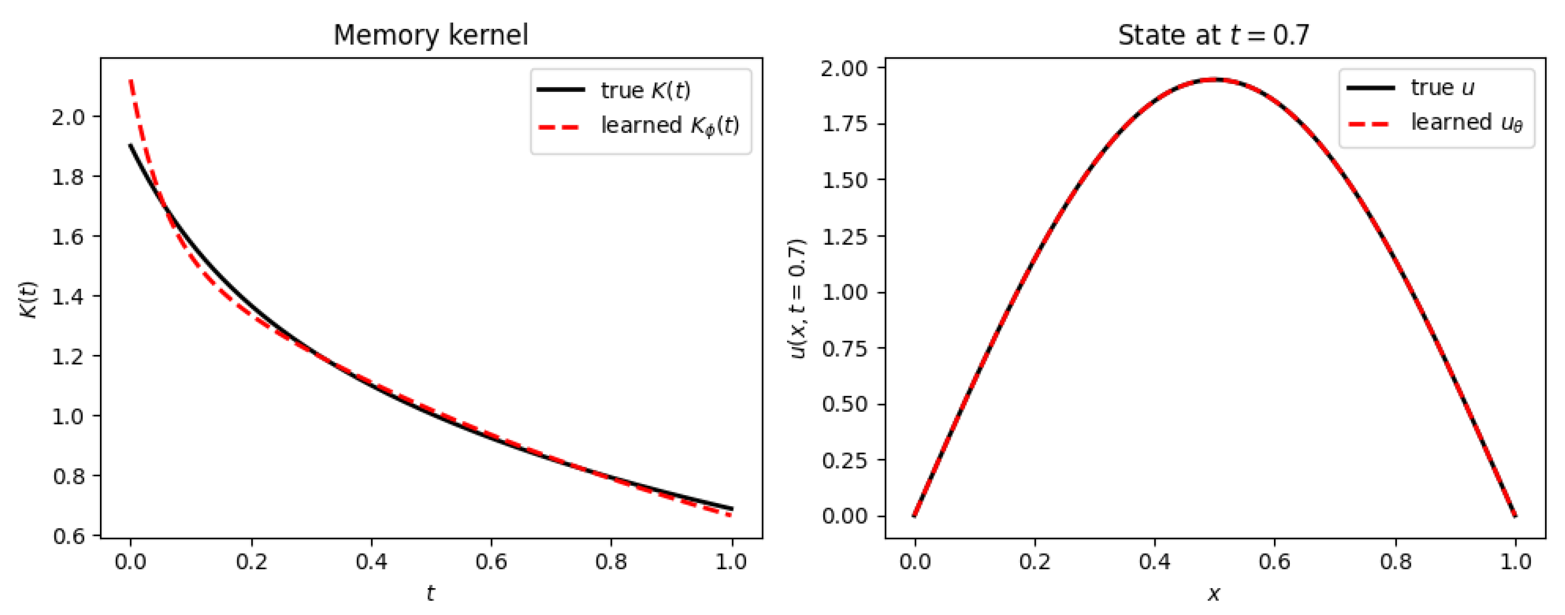
Figure 2.
Effect of the data-only warm-up and column-scaled regularization on Prony-kernel reconstruction. Left: original configuration. Right: final configuration. The architecture, benchmark, and governing equation are identical in both cases.
Figure 2.
Effect of the data-only warm-up and column-scaled regularization on Prony-kernel reconstruction. Left: original configuration. Right: final configuration. The architecture, benchmark, and governing equation are identical in both cases.

Figure 3.
Shape-constrained free spline (quadratically spaced knots) fit against the Prony ground truth. Kernel relative error: ; state error: .
Figure 3.
Shape-constrained free spline (quadratically spaced knots) fit against the Prony ground truth. Kernel relative error: ; state error: .
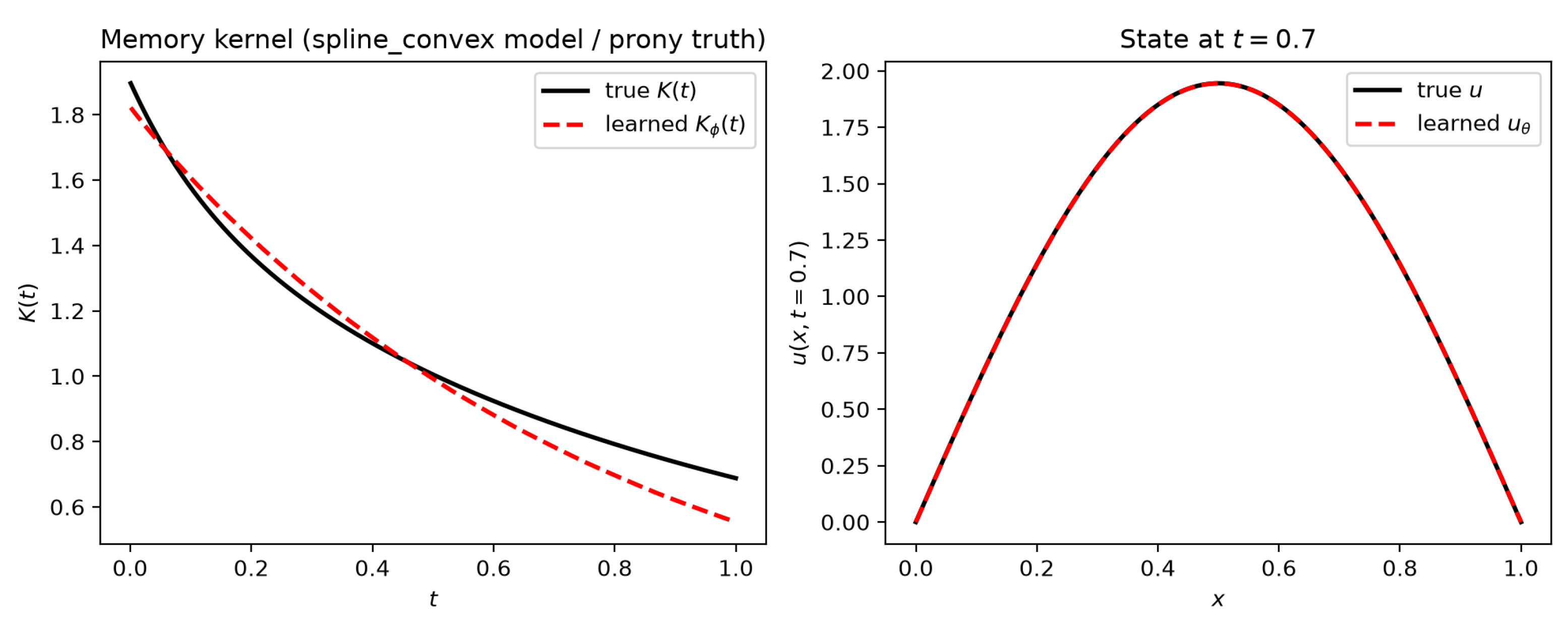
Figure 4.
Singular-value spectrum of the column-normalized Jacobian at the true parameters, for close versus well-separated decay rates. The close-rates spectrum decays markedly faster, reflecting a numerically rank-deficient direction in parameter space that the separated case largely avoids.
Figure 4.
Singular-value spectrum of the column-normalized Jacobian at the true parameters, for close versus well-separated decay rates. The close-rates spectrum decays markedly faster, reflecting a numerically rank-deficient direction in parameter space that the separated case largely avoids.
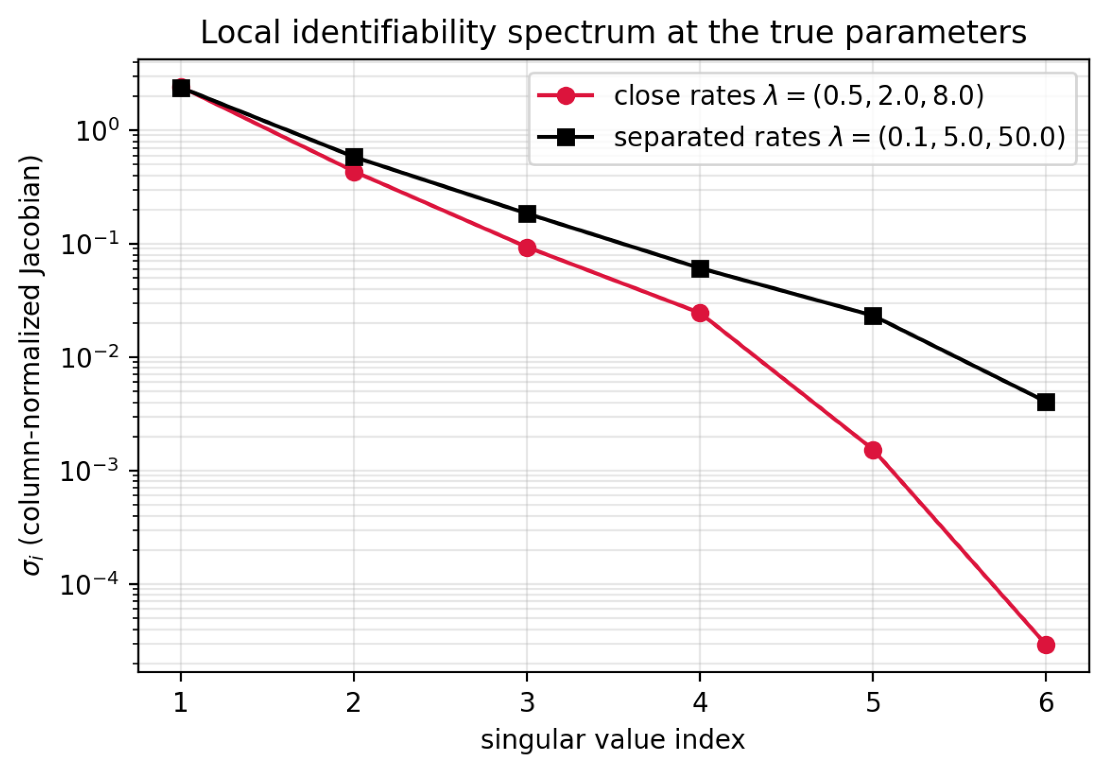
Figure 5.
Condition number of the column-normalized sensitivity Jacobian as a function of the separation ratio r in , on a logarithmic scale. The curve decreases monotonically across the entire sweep.
Figure 5.
Condition number of the column-normalized sensitivity Jacobian as a function of the separation ratio r in , on a logarithmic scale. The curve decreases monotonically across the entire sweep.
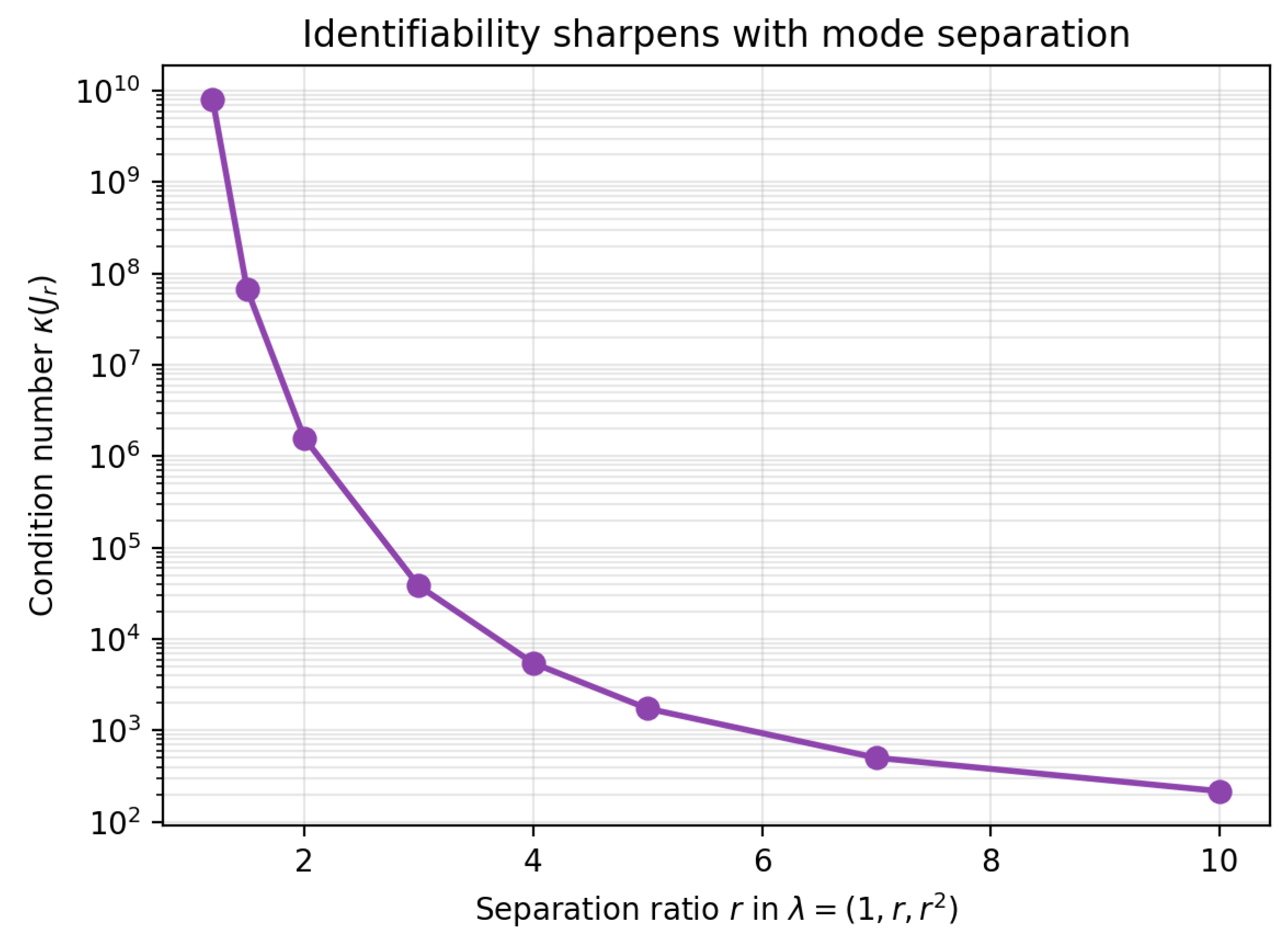
Figure 6.
Idealized Gauss–Newton/Laplace uncertainty at the true parameters (): individual rates (right) versus the propagated band (left).
Figure 6.
Idealized Gauss–Newton/Laplace uncertainty at the true parameters (): individual rates (right) versus the propagated band (left).
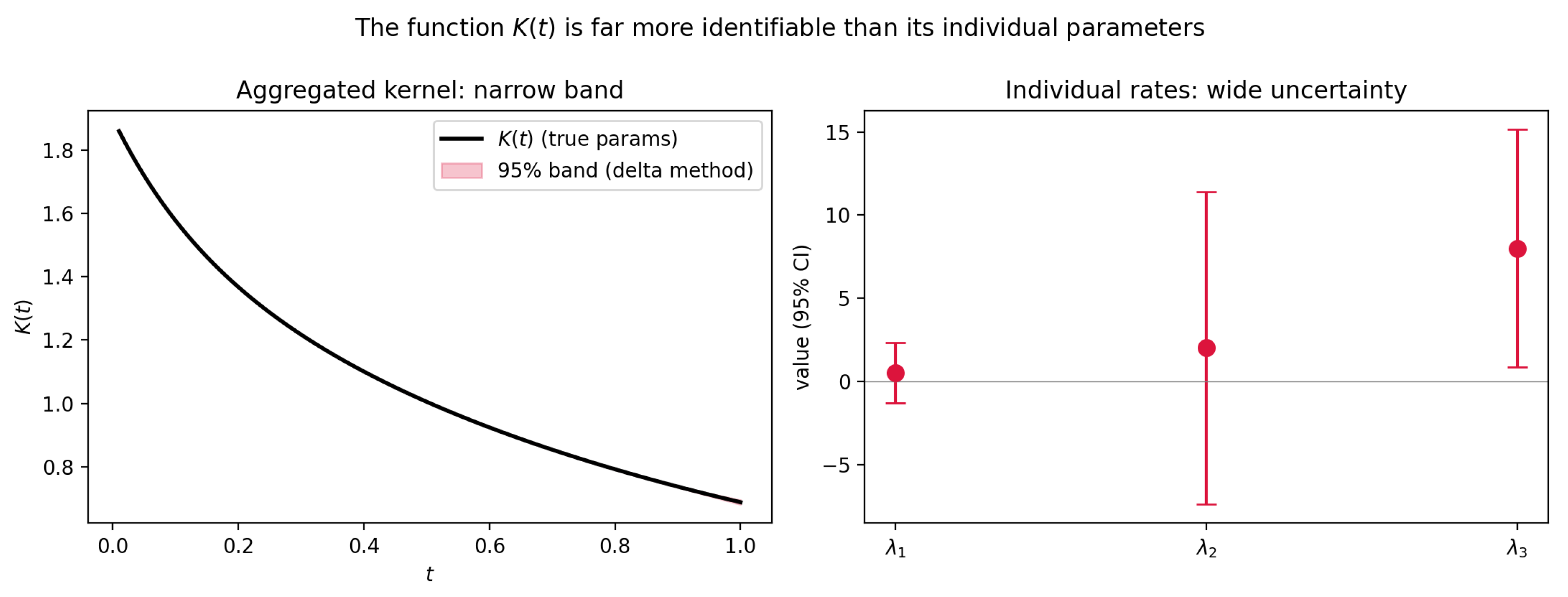
Figure 7.
Same analysis at the actual converged 12-mode fit, using the trained network’s own and achieved residual variance. Several rates carry uncertainty of hundreds to millions of percent; the aggregated band remains under .
Figure 7.
Same analysis at the actual converged 12-mode fit, using the trained network’s own and achieved residual variance. Several rates carry uncertainty of hundreds to millions of percent; the aggregated band remains under .
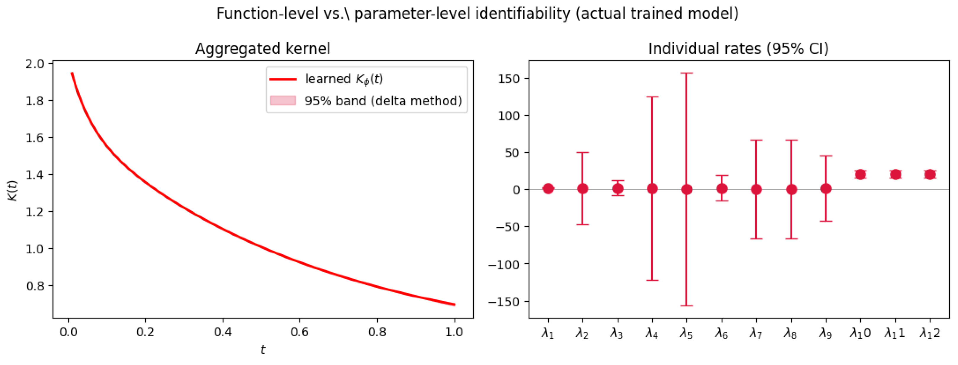
Figure 8.
Empirical, fully nonlinear validation: 8 independently trained replicates on identical data. Left: all 8 learned curves against the truth. Right: all 96 learned rates (8 replicates × 12 modes), pooled, spanning the entire admissible range.
Figure 8.
Empirical, fully nonlinear validation: 8 independently trained replicates on identical data. Left: all 8 learned curves against the truth. Right: all 96 learned rates (8 replicates × 12 modes), pooled, spanning the entire admissible range.
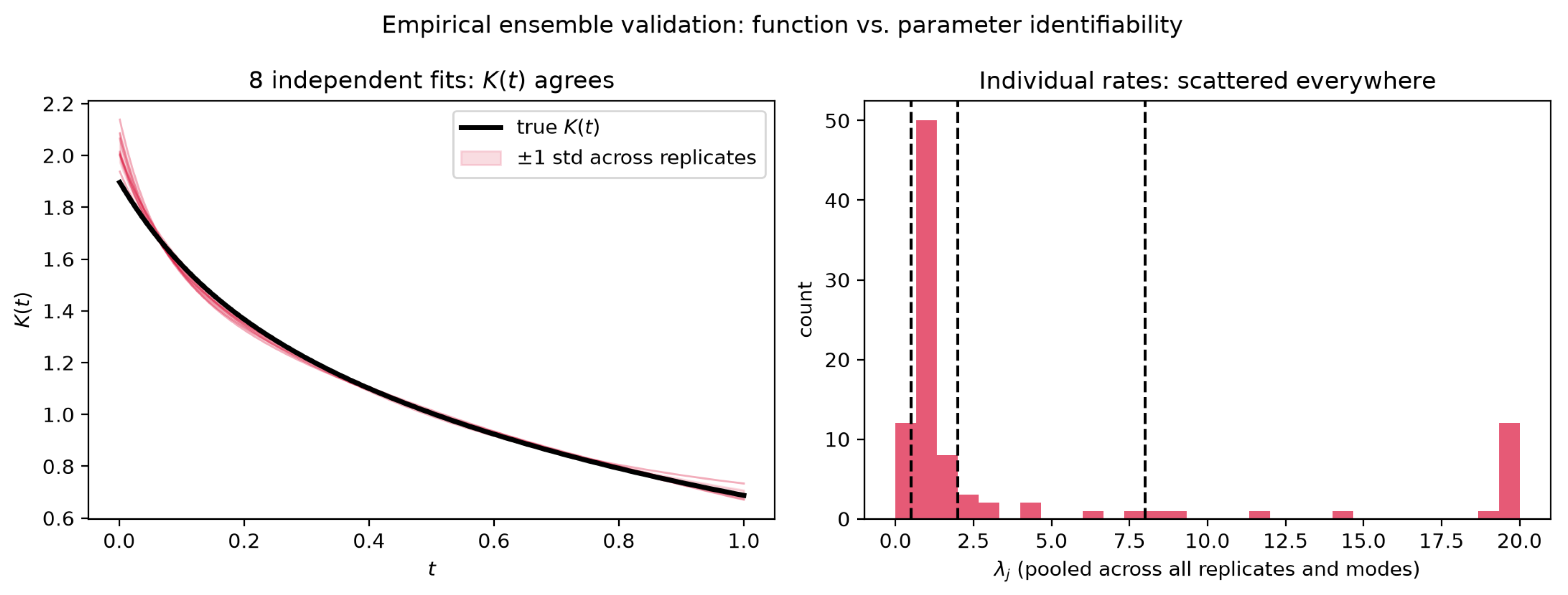
Figure 9.
Relative error versus observational noise level , for the state (), the kernel function (), and the Hungarian-matched Prony parameters (), full-scale run. Markers are means and error bars are one standard deviation over 10 replicates. The three curves sit at visually distinct scales throughout; the clearest monotonic response to noise is at , while stays within a saturated band across the whole sweep.
Figure 9.
Relative error versus observational noise level , for the state (), the kernel function (), and the Hungarian-matched Prony parameters (), full-scale run. Markers are means and error bars are one standard deviation over 10 replicates. The three curves sit at visually distinct scales throughout; the clearest monotonic response to noise is at , while stays within a saturated band across the whole sweep.
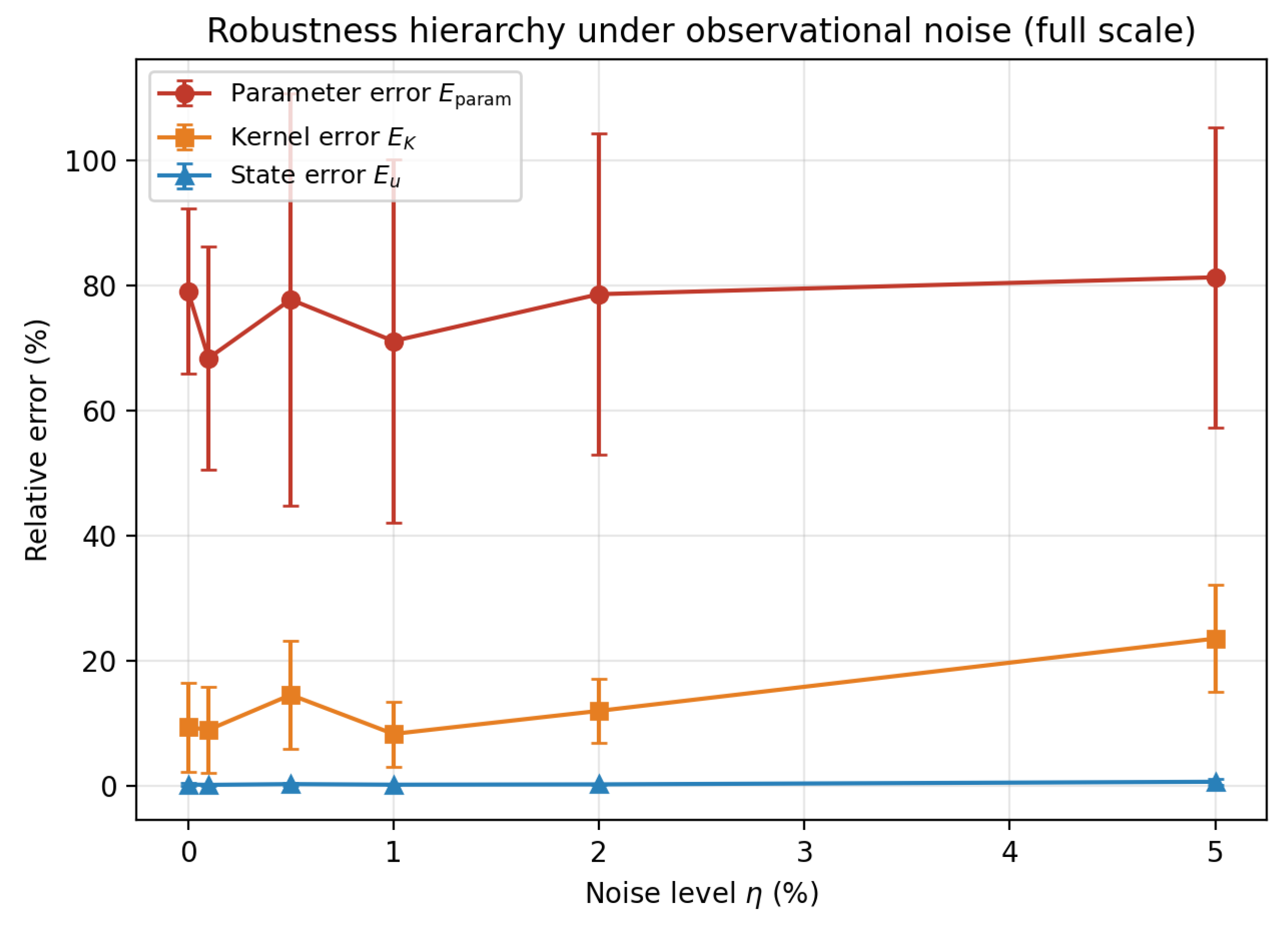
Table 1.
Kernel relative error under different configurations, all applied after the identifiability fix of Section 4.3. Every attempt to force and apart left the error flat or made it worse.
Table 1.
Kernel relative error under different configurations, all applied after the identifiability fix of Section 4.3. Every attempt to force and apart left the error flat or made it worse.
| Attempted change | M | Kernel error | ||
| Column-scaled ridge + data warm-up | 12 | 20 | 120 | – |
| Fewer modes (less redundancy) | 6 | 20 | 120 | |
| Fewer modes + wider bounds + more data | 4 | 40 | 250 | |
| More -refinement iterations | 12 | 20 | 120 |
Table 2.
Comparison between joint PINN reconstruction and direct kernel inversion using the exact state. State error is 0 by construction for the three exact-state rows, since no neural approximation is involved. Parameter error uses the top-3 Hungarian-matched metric described in the text; for PINN–VarPro we instead cite the individual-rate relative standard errors already established by the uncertainty analysis of Section 6, since the joint pairs from that run were not archived at the precision needed to recompute the same point-matching metric post hoc.
Table 2.
Comparison between joint PINN reconstruction and direct kernel inversion using the exact state. State error is 0 by construction for the three exact-state rows, since no neural approximation is involved. Parameter error uses the top-3 Hungarian-matched metric described in the text; for PINN–VarPro we instead cite the individual-rate relative standard errors already established by the uncertainty analysis of Section 6, since the joint pairs from that run were not archived at the precision needed to recompute the same point-matching metric post hoc.
| Method | State error | Kernel error | Parameter error |
| PINN–VarPro | – (Sec. 6) | ||
| Exact-state VarPro (ridge) | |||
| Exact-state VarPro (no ridge) | |||
| Exact-state Levenberg–Marquardt |
Table 3.
Effect of initialization and regularization on stretched-exponential kernel recovery. True parameters: .
Table 3.
Effect of initialization and regularization on stretched-exponential kernel recovery. True parameters: .
| Configuration | Loss behaviour | Learned | Kernel error |
| Initial (Prony-style ridge, single start) | increasing after round 3 | ||
| + multi-start grid on | still increasing | ||
| + no Tikhonov ridge (single mode) | monotonically decreasing |
Table 4.
Kernel families tested, ordered by local condition number at the true parameters where applicable. “Free parameters” counts -equivalent Prony configurations for comparability. The separated-rates Prony row is a sensitivity-only control (Section 5); it was not run end-to-end.
Table 4.
Kernel families tested, ordered by local condition number at the true parameters where applicable. “Free parameters” counts -equivalent Prony configurations for comparability. The separated-rates Prony row is a sensitivity-only control (Section 5); it was not run end-to-end.
| Kernel family | Free parameters | Condition number | Kernel error |
| Fractional (Caputo) | 1 | n/a (single parameter) | |
| Stretched exponential | 3 | ||
| Spline (shape-constrained, free) | 15 knots | n/a (no true params) | |
| Prony, separated rates (control) | 6 | 587 | — |
| Prony, close rates (benchmark) | 6 | 3– |
Table 5.
Local sensitivity comparison at the exact solution, no training involved. The column-normalized condition number is more than two orders of magnitude worse for closely spaced rates.
Table 5.
Local sensitivity comparison at the exact solution, no training involved. The column-normalized condition number is more than two orders of magnitude worse for closely spaced rates.
| Close rates | Separated rates | |
| Condition number (column-normalized) | ||
Table 6.
Condition number and pairwise cosine similarities of the column-normalized sensitivity Jacobian as a function of the mode separation ratio r in , fixed weights , no training involved.
Table 6.
Condition number and pairwise cosine similarities of the column-normalized sensitivity Jacobian as a function of the mode separation ratio r in , fixed weights , no training involved.
| r | ||||
| 2 | ||||
| 3 | ||||
| 4 | ||||
| 5 | ||||
| 7 | ||||
| 10 |
Table 7.
Effect of widening the observation window on the local conditioning of the stretched-exponential fit, evaluated at the true parameters with the same quadratic-in-t collocation scheme used in training (collocation count held fixed at ).
Table 7.
Effect of widening the observation window on the local conditioning of the stretched-exponential fit, evaluated at the true parameters with the same quadratic-in-t collocation scheme used in training (collocation count held fixed at ).
| (multiples of ) | Condition number | |
| 1 () | ||
| 2 () | ||
| 3 () | ||
| 5 () | ||
| 10 (18.2×) |
Table 8.
State, kernel, and parameter error as a function of the observational noise level , mean ± one standard deviation over 10 replicates. Full-scale run on Deucalion (MACC), matching Section 2. All values in percent.
Table 8.
State, kernel, and parameter error as a function of the observational noise level , mean ± one standard deviation over 10 replicates. Full-scale run on Deucalion (MACC), matching Section 2. All values in percent.
Disclaimer/Publisher’s Note: The statements, opinions and data contained in all publications are solely those of the individual author(s) and contributor(s) and not of MDPI and/or the editor(s). MDPI and/or the editor(s) disclaim responsibility for any injury to people or property resulting from any ideas, methods, instructions or products referred to in the content. |
© 2026 by the authors. Licensee MDPI, Basel, Switzerland. This article is an open access article distributed under the terms and conditions of the Creative Commons Attribution (CC BY) license (http://creativecommons.org/licenses/by/4.0/).
Copyright: This open access article is published under a Creative Commons CC BY 4.0 license, which permit the free download, distribution, and reuse, provided that the author and preprint are cited in any reuse.