

Submitted:
10 September 2026
Posted:
13 September 2026
You are already at the latest version
Abstract
Accurate wind resource estimation in complex environments, such as the Colombian Caribbean, is challenging due to air–sea heat fluxes and nonlinear atmospheric dynamics. This systematic review and meta-analysis synthesized empirical evidence from 49 studies to evaluate whether advanced forecasting architectures (artificial intelligence, ensemble, and hybrid models) systematically outperform classical physical models. The pooled random-effects estimate indicated an overall reduction in reported forecasting error (\(g = -1.6874\)), though heterogeneity was extreme (\(I^2 = 99.99\%\)). Categorical meta-regression revealed no statistically significant advantage for advanced architectures over physical models (\(\beta_1 = 0.2558\), \(p = 0.9339\)). Mixed-effects meta-regression identified Sample Size (\(N > 10{,}000\)) as the primary significant moderator, with the final model explaining 40.47% of between-study variability (\(R^2_{\text{analog}} = 40.47\%\), reducing residual variance from \(\tau^2 = 2.5102\) to \(\tau^2 = 1.4943\)). Metric-specific contrasts indicated that physical and AI architectures are statistically indistinguishable, whereas hybrid models yielded lower pooled effects. classical physical models remain a reliable, stable reference framework, whereas AI and hybrid approaches demonstrate advantages only in specific, non-generalizable settings. These findings challenge the assumption of universal superiority for AI-based wind forecasting in complex coastal domains.
Keywords:
wind power forecasting
; meta-analysis
; complex terrain
; coastal wind dynamics
; artificial intelligence
; hybrid models
; physical models
; heterogeneity
; meta-regression
1. Introduction
The transition to a decarbonized energy mix requires the integration of high-power-density sources and reliable management systems. Carbon dioxide emission analyses show that mitigation does not follow a linear relation between infrastructure and pollutant reduction; in high-emission regimes, systemic deficiencies limit proportional gains [1,2]. By the end of 2024, wind and solar reached of global electricity production, with wind technology standing out due to its rapid response to grid disturbances [3,4]. Further increases depend on a synergistic combination of technical capabilities and context-adapted management models [5,6,7].
In South America, realistic representation of climatic conditions challenges numerical models due to the region’s southern extent and heterogeneous topography, among them the Andes and the Amazon [8]. Water and atmospheric variability depends strongly on sea surface temperature and mountain elevation, which shape circulation and partition moisture sources [9,10]. Despite advances in environmental data processing, state-of-the-art systems such as CMIP6 (Coupled Model Intercomparison Project Phase 6) models still exhibit systematic biases in precipitation simulation and in the representation of atmospheric circulation processes [11,12].
In the Colombian Caribbean, interaction between the Caribbean Low Level Jet (CLLJ), coastal orography, and estuarine dynamics produces nonlinear wind blocking and shear effects, which undermine stability assumptions in conventional statistical forecasting methods [13]. This interaction generates vertical wind profiles that violate Hellmann’s Power Law, widely used for wind speed extrapolation [14]. Night jets and variable coastal roughness add residual variance that simple statistical models fail to capture, which increases short-term estimation error.
The complexity of the region extends to the Caribbean convergent margin, where contourite systems shaped by subduction tectonics and strong bottom currents reflect coupled oceanic and tectonic controls on slope dynamics, with indirect effects on coastal atmospheric circulation relevant to wind energy assessment [15]. In this context, wind power estimation benefits from improved representation of atmospheric and environmental variables, and a diversity of modeling approaches.[16,17,18].
Contemporary literature on wind profile and potential estimation models reveals a theoretical fragmentation where numerical optimization frequently precedes geographical contextualization. Recent evaluative studies suggest a shift in metric preference, with some authors arguing that the Mean Absolute Percentage Error (MAPE) exhibits limitations with near zero values, that normalized metrics, such as nRMSE and nMAE, effectively address [19,20]. However, MAPE continues to serve as a foundational metric upon which these advanced normalized methodologies are constructed. While classical physical and statistical approaches maintain linear efficiency, advanced methods utilize the universal approximation theorem to model complex interactions in short-term horizons [21,22,23,24]. The current knowledge gap resides in the lack of specificity for coastal regions influenced by trade winds, where fragmented data infrastructure and extreme environmental conditions degrade telemetry and subsequent decision-making processes [25,26,27,28,29,30,31,32,33,34].
The wind energy forecasting in these environments requires approaches that enable the identification of effective architectures. This work evaluates the main families of models used in wind potential estimation, such as classical and advanced methods in coastal and complex regimes. Direct comparison across studies remains infeasible due to diverse experimental designs, as each study defines its own reference condition through physical models, statistical baselines, or machine learning approaches; this leads to non-standardized control model definitions across the corpus. To address this limitation, metrics optimized for higher values and metrics optimized for lower values are rescaled to a common direction, such that lower values consistently indicate better performance. This enables a directionally consistent synthesis within predefined architecture, comparator-design, and metric-family strata, while the original structure of each experiment is preserved.
The key contributions of this study are summarized as follows:
- A random-effects meta-analysis that synthesizes evidence from validated wind forecasting studies conducted in complex terrain and coastal environments, providing an exploratory descriptive assessment of the available evidence and a statistical framework for subsequent subgroup and moderator analyses.
- A hierarchical moderator analysis that systematically evaluates the influence of methodological and study-related factors on variability in reported forecasting performance, providing a statistical framework for investigating the sources of between-study heterogeneity.
- An evidence-based reassessment of forecasting architecture performance showing that a categorical meta-regression does not support a systematic advantage of Advanced (AI, Hybrid) architectures over Classical Physical models (), that Classical Physical models exhibit the largest observed average performance improvement among the evaluated architecture categories, and that architectural category alone explains only a small share of the observed heterogeneity, highlighting the need to jointly consider architecture, evaluation metric, and study characteristics when interpreting forecasting effectiveness.
The architectures considered in this work are described as follows:
-
Classical Models: Foundational Approaches, traditional methodologies that laid the foundations in wind forecasting, characterized by a deterministic approach or the use of linear mathematical statistics.
- 1.
- Pure Physical (Deterministic) Models: These models use meteorological data such as temperature, atmospheric pressure, surface roughness, and the presence of local obstacles to characterize wind flow. Through this processing of environmental variables, the wind is scaled to the turbine hub height to estimate energy production.
- 2.
- Traditional Statistical Models: These models perform time series analysis to identify linear stochastic patterns in historical wind or power data. Autoregressive models, such as AutoRegressive Moving Average (ARMA) and AutoRegressive Integrated Moving Average (ARIMA), and persistence models are the most representative examples. Their main advantage is computational efficiency and high accuracy over very short time horizons (minutes to a few hours).
-
Advanced Models: Emerging Technologies encompass architectures designed to capture the non-linear, chaotic, and intermittent nature of the wind, overcoming the limitations of classical approaches.
- 1.
- Artificial Intelligence (AI)-Based Models: These models map complex, nonlinear relationships between input variables, weather data or historical Supervisory Control and Data Acquisition (SCADA) records, and power output using machine and deep learning algorithms.
- 2.
- Ensemble Models: This architecture combines the predictions of multiple base models to improve overall accuracy, reduce variance, and mitigate time bias. It encompasses techniques such as gradient boosting and weighted aggregation of different neural networks.
- 3.
- Hybrid Models: These combine techniques of different natures to exploit strengths and mitigate individual weaknesses. Models that combine a physical model with intelligent schemes such as machine learning, deep learning, and metaheuristic optimization are currently dominant.
2. Materials and Methods
The synthesis seeks to identify configurations that minimize uncertainty under coastal and complex atmospheric regimes. Observed variability across studies highlights the limitations of universal model ranking and supports context-dependent evaluation. The study follows a pre-registered protocol on the Open Science Framework (OSF) entitled: “Protocol for the review and meta-analysis of the accuracy of Advanced Methods (AI, Ensemble and Hybrid) versus Classical Methods (Pure Physical and Statistical) for estimating wind power at onshore and offshore sites influenced by coastal or trade wind dynamics” [35].
This research is framed within the PICO (Population, Intervention, Comparison and Outcome) framework with the objective of determining whether, in the context of wind resource estimation at complex onshore and offshore sites influenced by coastal or trade wind regimes (P), the implementation of “Advanced” computational architectures based on artificial intelligence, ensemble systems, and hybrids (I) exhibits superior predictive accuracy compared to “Classical” reference models based on linear physical and statistical principles (C), quantified by the reduction of error and bias (O). The analysis incorporates a hierarchical meta-regression to identify the impact of technical moderators such as architecture, sample size, and metric type on the variability of the observed effect. Although the PICO framework and the search strategy (Table 1) were designed to admit both physical and traditional statistical reference models under the Classical category, no study meeting the final eligibility criteria used a purely statistical model as its comparator; the Classical category in the final corpus is therefore constituted exclusively by Pure Physical models, and any statement about “Classical” performance in this study should be read as applying specifically to physical reference models. This absence is reported explicitly in Section 4.1 rather than treated as equivalent to a null statistical-model condition.
Eligible studies include advanced models (artificial intelligence, hybrid systems, or ensembles) and classical models (physical or statistical) that report sufficient performance metrics for effect size computation. Technical reports, conference papers, and studies not based on coastal or complex terrain conditions are excluded. The search is restricted to English-language publications from 2020 to 2025 to ensure that the comparisons reflect the current state of wind forecasting methods.
The identification of scientific literature was carried out through a systematic search of the Scopus and Web of Science (WoS) databases, with the final query performed on 29 January 2026. To ensure the integrity of the bibliographic corpus, a reverse search was applied to the reference lists of the selected articles. The search strategy used Boolean syntax (AND, OR) and targeted descriptors across three thematic axes: wind power estimation, coastal wind dynamics or complex terrain, and model architectures. To avoid loss of relevant information, variations of key terms were incorporated into the queries. Detailed information on the search strings is provided in Table 1.
The analysis prioritized studies that evaluates wind estimation models in complex terrain or coastal environments characterized by high spatial and temporal variability. Statistical comparability across studies required the availability of effect sizes (ES) and their standard errors (SE); when not reported, these were derived from available summary statistics to enable quantitative synthesis. Study selection followed a dual independent review process, with discrepancies resolved by a third expert in computational meteorology. Abstract screening and record management were supported using the revtools package for bibliographic processing [36], and final inclusion depended on the completeness of data required for effect size computation.
Data synthesis integrated the Meta-Essentials algorithmic framework with custom Python routines to optimize the processing of large volumes of information. The analysis employed random-effects models based on the DerSimonian–Laird inverse-variance weighting method, with confidence and prediction intervals computed using Student’s t-distribution ( degrees of freedom). The workflow included standard tests of heterogeneity (Q, , and ), Egger’s regression, and Rosenthal/Fisher fail-safe analyses, among other methods described below [37,38,39]. Within this framework, the following hypotheses are defined:
- (Alternative Hypothesis): Advanced forecasting models exhibit a significantly larger magnitude of performance improvement compared to classical models, as reflected by more negative standardized effect sizes , indicating greater reductions in forecasting error.
- (Null Hypothesis): There is no statistically significant difference in standardized effect sizes between advanced and classical models ().
The evaluation of these hypotheses is conducted within a meta-analytic framework that compares effect sizes across model categories. As an initial exploratory step, pooled subgroup estimates are computed for classical and advanced architectures to characterize general patterns of performance differences.
Formal inference regarding is based on a categorical meta-regression, where architectural category (Classic: Physical, Statistical; Advanced: Hybrid, AI, Ensemble) is included as a primary moderator of the effect size. The statistical significance of the corresponding regression coefficient is used to evaluate whether advanced architectures systematically differ from classical physical models in terms of standardized performance improvement.
Given the expected presence of substantial between-study heterogeneity , additional technical moderators such as sample size, metric type, and input configuration are incorporated to account for structural sources of variability. This hierarchical specification enables the identification of conditions under which performance differences are amplified or attenuated, ensuring that inference is not based solely on aggregated global means.
2.1. Meta-Analysis Inputs: Effect Size and Standard Error
Meta-analysis is established as a fundamental method for the quantitative accumulation of knowledge. It differs from a narrative review because it provides a quantitative assessment of the relationship between variables or the effectiveness of an intervention. As in any empirical study, research begins with definition of the research question, which delimits the scope of constructs and interventions under analysis. The choice of effect size (ES) measure depends on the research question and field conventions. Common measures include correlation coefficients and standardized mean differences, as well as regression coefficients, survival rates, risk ratios, and odds ratios [40].
In [41], the conclusions of Johnson, Mullen, and Salas (1995) are analyzed. Their claim that the meta-analysis methods of Hunter and Schmidt (1990) produce anomalous results stems from the use of an inadequate formula for standard error rather than methodological flaws. It is established that, when the correct procedures are used, the results of the three compared methods are consistent. The choice of the effect size measure and its standard error addresses the need to standardize the numerical results of performance metrics, in this case, the focus is on wind resource estimation models. In this study, the standardized mean difference under the estimator of Hedges [42,43] is selected, and other metrics such as relative risk (RR, normally also used by means of [44,45]) are discarded in order to preserve the quantitative nature of the estimation errors and subject all models to the same comparative regime [46].
To ensure the validity of this synthesis, it is imperative to use error formulas consistent with the population variance. Hedges’ corrected g is well known for behavior that reflects less bias, due to the correction factor that is added to Cohen’s d. It is recognized that inaccuracies in the calculation of the standard error, such as the omission the correction factor for the number of studies, generate systematic overestimations that invalidate the statistical inference. Consequently, the integration of results is performed through weights based on the inverse of the variance, which mitigates the bias derived from sampling error [47,48].
2.2. Quantitative Synthesis and Effect Size Calculation
The methodological framework adopts the standardized mean difference (SMD) to harmonize results across studies. Hedges’ g serves as the primary effect size estimator (see Equation (1)). In this context, the “proposed” group denotes the primary forecasting architecture or configuration under investigation, whereas the “control” group represents the reference benchmark or baseline.
However, it is important to note that the effect sizes are not derived from raw observational distributions, but rather reconstructed from reported aggregate error metrics. As a result, Hedges’ g in this framework should be interpreted as a within-study standardized index of relative predictive performance gain over a given baseline, rather than a classical standardized mean difference based on underlying sample-level variance.
2.2.1. Standardization and Scalar Comparability
The pooled standard deviation (see Equation (2)) provides the within-study scaling factor required for the calculation of standardized mean differences, allowing effect estimates reported in different numerical scales to be expressed in a common standardized form. Given that the corpus includes performance measures reported in heterogeneous physical units, such as , , and , as well as diverse error-based metrics including RMSE, MAE, and MAPE, enables normalization of study-specific contrasts within each individual comparison.
As the denominator in Equation (1), rescales the mean difference into standard deviation units, reducing dependence on the original measurement scale, although differences in metric definitions and evaluation objectives are not fully resolved. The correction factor J depends on the degrees of freedom , where and are the sample sizes of the two groups. The term is the subtraction of two degrees of freedom that reflects the estimation of the two group means required to compute the pooled variance.
Although Hedges’ g standardizes study-specific performance differences, effect sizes reconstructed from heterogeneous evaluation metrics, including absolute physical measures, Relative Performance metrics, correlation coefficients, and probabilistic metrics, are not fully commensurable across measurement domains. Therefore, the overall pooled analysis is interpreted as an exploratory descriptive synthesis that summarizes the distribution of standardized effects across the available evidence, rather than as definitive statistical evidence supporting direct comparisons among heterogeneous metric families. Consequently, the interpretation of forecasting performance is primarily based on the subsequent stratified meta-analyses and hierarchical meta-regression, in which metric families are analyzed separately.
2.2.2. Variance Estimation and Weighting Scheme
The DerSimonian–Laird (DL) estimator computes the between-study variance . The DL method offers a non-iterative, moment-based approach that does not require a specific distribution for the random effects. Within the random-effects framework, the between-study variance contributes to the weighting scheme. The adjusted study weights and the overall effect are then calculated as follows:
This specification accounts for both within-study variance and between-study variability . Consequently, effect sizes vary across studies, which is appropriate for this analysis where we have different predictive objectives, such as Wind Power Output (WPO), Wind Speed Profile (WSP), and Atmospheric Conditions (ATM). The standard error of g quantifies the uncertainty for each individual estimate. The within-study variance is defined as the square of the standard error:
2.2.3. Precision and Interval Estimation
The confidence interval (CI), which quantifies the uncertainty in the average effect size for the gobal mean is based on the variance of the summary estimate, . Using a t-distribution with degrees of freedom, the CI is:
The prediction interval (PI) accounts for the expected dispersion of a future observation, in addition to the uncertainty of the average, there is the real dispersion that exists between the different studies analyzed, the variability :
2.2.4. Pooling Methodology
The choice between pooling methods depends on how the true effect is defined, the idealized performance of the prediction model if it were measured without sampling error. In a fixed-effects model, the true effect is an invariant constant; it is assumed the model performs identically across all studies, and any variation in observed performance is attributed solely to random noise. In contrast, the random-effects model treats the true effect as a random variable. Here, each study estimates its own specific true effect, acknowledging that model performance can genuinely differ between studies due to methodological heterogeneity.
2.3. Hypothesis Validation and Meta-Regression
2.3.1. Hypothesis Validation Through Architecture-Based Meta-Regression
To evaluate the proposed hypotheses, a random-effects meta-regression was applied to test whether Advanced forecasting architectures exhibit different standardized effect sizes compared with Classic physical models. The general random-effects meta-regression is expressed in Equation (8):
where denotes the observed effect size for study k, represents the intercept, corresponds to the estimated regression coefficients, represents the within-study sampling error (), and represents the residual between-study heterogeneity component () [49].
To formally test the proposed hypothesis, the model was specified using architecture category as the comparison variable:
where represents the Hedges’ g effect size of study i. The intercept represents the estimated pooled effect size of the reference category, defined as Classic physical models. The coefficient represents the difference in standardized effect size between Advanced and Classic architectures. The binary variable was defined as for AI-based and hybrid models and for physical models.
Consequently, the coefficient associated with architecture estimates the contrast shown in Equation (10):
A negative and statistically significant value of would provide evidence supporting the alternative hypothesis (), indicating that Advanced architectures achieve larger reductions in forecasting error compared with Classic physical approaches. Conversely, a non-significant coefficient would indicate insufficient statistical evidence to support a systematic difference between the two architectural categories.
2.3.2. Hierarchical Meta-Regression for Explaining Study-Level Variability
While the hypotheses and assess the existence of systematic differences in performance between advanced and classical forecasting models, this does not capture the underlying mechanisms that generate such differences. To address this limitation, a meta-regression is employed to explore the conditions under which these performance gaps emerge, vary in magnitude, or diminish across studies. This part of the analysis investigates how methodological and technical factors such as model architecture, sample size, and evaluation metric structure contribute to the observed variability in standardized effect sizes , thereby providing a deeper explanation of the mechanisms behind the global effect.
The evaluation of moderator relevance is based on three complementary criteria: variance reduction, residual heterogeneity reduction, and statistical significance of individual moderator coefficients.
-
Explanatory Power (Analog ; proportional variance reduction): The explanatory contribution of a moderator structure is evaluated through the proportional reduction in the estimated between-study variance component after extending an unconditional random-effects model with moderator variables. This approach follows the variance-explained framework described by Raudenbush and Bryk, where the proportion of variance explained is obtained by comparing the variance component of an unconditional model with the residual variance component of a conditional model [50].Adapting this variance reduction principle to the meta-analytic setting, the Analog measure is defined as:where represents the estimated between-study variance from the unconditional random-effects meta-analysis model without moderators, and represents the residual between-study variance estimated from the mixed-effects meta-regression model after including the moderator structure. Therefore, Equation (11) is considered as a continuous measure of the proportion of between-study variance accounted for by the included moderators. Higher values indicate greater explanatory contribution, although interpretation must consider model complexity and the persistence of residual heterogeneity.
- Residual Heterogeneity Reduction (): Beyond the proportional reduction quantified by Analog , moderator performance is further evaluated through the absolute reduction in the estimated between-study variance between the unconditional and conditional models as shown in Equation (12):where and represent the estimated between-study variance components before and after moderator inclusion, respectively. The absolute reduction quantifies the reduction in unexplained variance, while Analog expresses this reduction proportionally relative to the baseline variance. Both measures are interpreted comparatively across moderator structures, considering explanatory contribution and model parsimony.
- Statistical Significance of Moderators: Moderator coefficients are evaluated through hypothesis tests using conventional significance levels (). Statistical significance is interpreted jointly with explanatory power and variance reduction, as relevant moderators may not achieve individual significance under limited statistical power, sparse subgroup representation, or correlated moderator structures.
3. Results
Figure 1 illustrates the overlap between the databases used; the complementary use of both is justified to ensure coverage of the technical literature in engineering and atmospheric sciences (Intersection Detected: 3253, Unique Universe : 5671, Overlap Rate: ).
The workflow consisted of three filtering stages: abstract selection (F1), full-text evaluation (F2), and removal of remaining duplicates and methodological verification (F3). The quantitative results, detailed in Table 2, indicate an initial pool of 8,924 records. During phase F2, the exclusion of manuscripts due to a lack of error metrics or insufficient description of the field context reduced the count from 140 to 59. Finally, in stage F3, the removal of duplicates (10 cases) and a technical audit of the statistical procedures resulted in a final synthesis of 49 studies.
Scopus provided the largest volume of records . The systematic selection process, from initial identification to final inclusion, appears in the PRISMA 2020 flowchart in Figure 2.
3.1. Study Characteristics
The publication dynamics and geographic focus demonstrate a growing interest in wind energy forecasting within areas with complex topography. The period of selection of relevant literature revealed that there is substantial variability in terms of estimation horizons, terrain complexity descriptors, and performance metrics; this methodological heterogeneity is an intrinsic condition of the corpus that must be addressed a priori.
The statistical synthesis (Table 3), performed using a random-effects model including 49 independent studies, yielded a combined effect size of with a 95% confidence interval ranging from to , this estimated effect was statistically significant . Considering the adopted effect size formulation, where negative Hedges’ g values indicate lower standardized prediction errors for the proposed forecasting architectures relative to the corresponding reference models, the estimated average effect suggests an overall improvement in predictive performance across the analyzed literature.
However, the interpretation of this average effect requires consideration of the substantial variability among the included studies. The estimated 95% prediction interval ranged from to , describing the expected dispersion of true effect sizes across future comparable applications. The breadth of this interval is consistent with the methodological and contextual diversity of the analyzed studies, including differences in forecasting objectives, model configurations, terrain characteristics, evaluation procedures, and reported performance metrics. The observed heterogeneity is the most prominent characteristic of the analyzed corpus, a Cochran’s Q statistic (, ) and an () indicate that nearly all observed variability originates from genuine differences among studies rather than sampling uncertainty. The estimated between-study variance () further confirms substantial dispersion in the underlying effect sizes. Consequently, although the negative summary effect indicates an overall tendency toward improved predictive performance of the evaluated forecasting architectures relative to the reference models, the magnitude of this improvement should be considered dependent on the specific characteristics of each application context [52].
3.2. Risk of Bias in Studies
Publication bias was assessed using multiple diagnostics (see Table 5). Egger’s regression showed no significant funnel plot asymmetry (, , ), whereas the Begg & Mazumdar rank correlation test suggested potential small-study effects (, ). Thus, evidence of publication bias remains mixed. The Rosenthal Fail-Safe N () exceeded the threshold (255), indicating robustness of the overall statistical significance. Similarly, the Orwin Fail-Safe test estimated that approximately additional studies with a mean effect size of zero would be required to reduce the pooled effect to the predefined trivial threshold (). These results suggest robustness of the representative pooled effect estimate against hypothetical null-effect studies; however, they do not exclude the presence of small-study effects or the substantial between-study heterogeneity observed [53,54,55].
The Normal Quantile Regression confirms deviations from the expected normal distribution. The estimated slope of and intercept of indicate systematic departures from theoretical normal quantiles. The QQ plot (see Figure 4) corroborates this result, as the residuals exhibit an approximately linear pattern with mild deviations, this suggests a slightly higher concentration around the mean, a heavy-tailed behavior that characterizes a leptokurtic distribution.
The discrepancy between high statistical significance and extreme predictive uncertainty suggests that the global average is an insufficient descriptor of the current state of the art.
3.3. Moderator Analysis and Hierarchical Meta-Regression
The substantial variance identified in the primary analysis necessitates a systematic decomposition through hierarchical meta-regression. This process helps to verify whether the observed dispersion of effects is due to the intrinsic complexity of atmospheric phenomena or to specific methodological artifacts and data processing scales.
3.3.1. Taxonomic Distribution and Baseline Specification
The corpus taxonomy (see Table 6) indicates a predominance of advanced architectures, which constitute of the sample (). Classical physical models account for of the dataset (), while no studies are classified under the purely Statistical category. This distribution establishes the comparative structure for evaluating architecture as a potential moderator of forecasting performance. The presence of two ensemble studies ( of the corpus) reflects the emerging adoption of ensemble strategies in wind forecasting, although their limited representation prevents an independent architecture-level meta-analytic comparison. Consequently, the main comparative analysis focuses on the three sufficiently represented architecture categories: Hybrid, Physical, and AI, distributed across the defined intervention groups (Classic and Advanced).
The results summarized in Table 7 and illustrated in the forest plot (see Figure 5) indicate substantial overall improvements in forecasting performance, although important differences emerge across architectural subgroups when considering effect magnitude, statistical stability, and robustness. AI-based models demonstrated a substantial observed improvement but this subgroup presents the highest dispersion and the widest prediction interval, indicating greater uncertainty in the generalization of performance gains; additionally, the failsafe-N value of 80.4 relative to a threshold of 105 suggests limited robustness. In contrast, physical models showed a slightly larger observed effect, although substantial heterogeneity persisted, this subgroup displayed lower between-study dispersion and a narrower prediction interval, with borderline robustness (failsafe-N = 78.8; threshold = 80). Hybrid approaches show the weakest observed effect, with low robustness (failsafe-N = 6.0; threshold = 80).
Despite differences in point estimates, the substantial overlap in confidence intervals across architectural categories, together with uniformly extreme heterogeneity, suggests that architecture alone does not adequately explain the observed variability in forecasting performance. Physical models yielded the largest estimated effects and comparatively lower between-study dispersion than AI models, although both subgroups remained highly heterogeneous. In contrast, hybrid models exhibited weaker effects and limited robustness after adjustment.
Using the mixed-effects meta-regression model described in Section 2.3.1, the architecture category was evaluated as a binary moderator, where represented AI-based and hybrid approaches and represented Classic physical models. The estimated intercept, corresponding to the Classic group effect, was:
The moderator coefficient, representing the difference between Advanced and Classic architectures, was:
Therefore, the estimated pooled effect for the Advanced group was calculated as:
The estimated difference between architecture categories was not statistically significant, with a 95% confidence interval ranging from -5.7907 to 6.3023 and a corresponding test statistic of .
The hypothesis evaluation assumed that Advanced architectures would produce larger improvements than Classic physical approaches, represented by a more negative standardized effect size:
However, the estimated moderator coefficient was positive (), indicating that Advanced architectures exhibited a less negative average effect size compared with Classic approaches:
Nevertheless, the confidence interval around the moderator coefficient included zero, indicating that the observed difference between groups was not statistically distinguishable. Therefore, the mixed-effects meta-regression did not provide evidence supporting the hypothesis that Advanced architectures achieve greater performance improvements than Classic physical models. Consequently, was not supported, and the null hypothesis could not be rejected.
The estimated residual heterogeneity after including the architecture moderator was , indicating that a substantial proportion of between-study variability remained unexplained by architectural category alone. This suggests that additional methodological factors may contribute to the observed differences in effect sizes. Table 8 provides further context by illustrating the distribution of architectural categories across evaluation metric families, highlighting potential sources of confounding and heterogeneity in architecture-based comparisons.
The dataset is not evenly distributed across architectural categories and metric families. Classic (Physical) models () are predominantly evaluated using Absolute Error Metrics (AEM; 11 studies), whereas Advanced approaches cover a broader range of evaluation criteria. AI models represent the largest Advanced subgroup (), with most studies using AEM (11 studies) but additional representation across CRM, PBM, and PRM. Hybrid models () show greater metric diversity, including AEM (7 studies), CRM (1 study), PBM (3 studies), and PRM (3 studies). The Ensemble category () remains insufficiently represented for independent architectural inference.
3.3.2. Analysis of Group-Specific Results
The subgroup analysis in Table 9 indicates that the magnitude and consistency of the standardized effects vary across metric families. Since each family captures a different aspect of forecasting performance, separate analyses provide additional insight into the robustness and generalizability of the observed improvements.
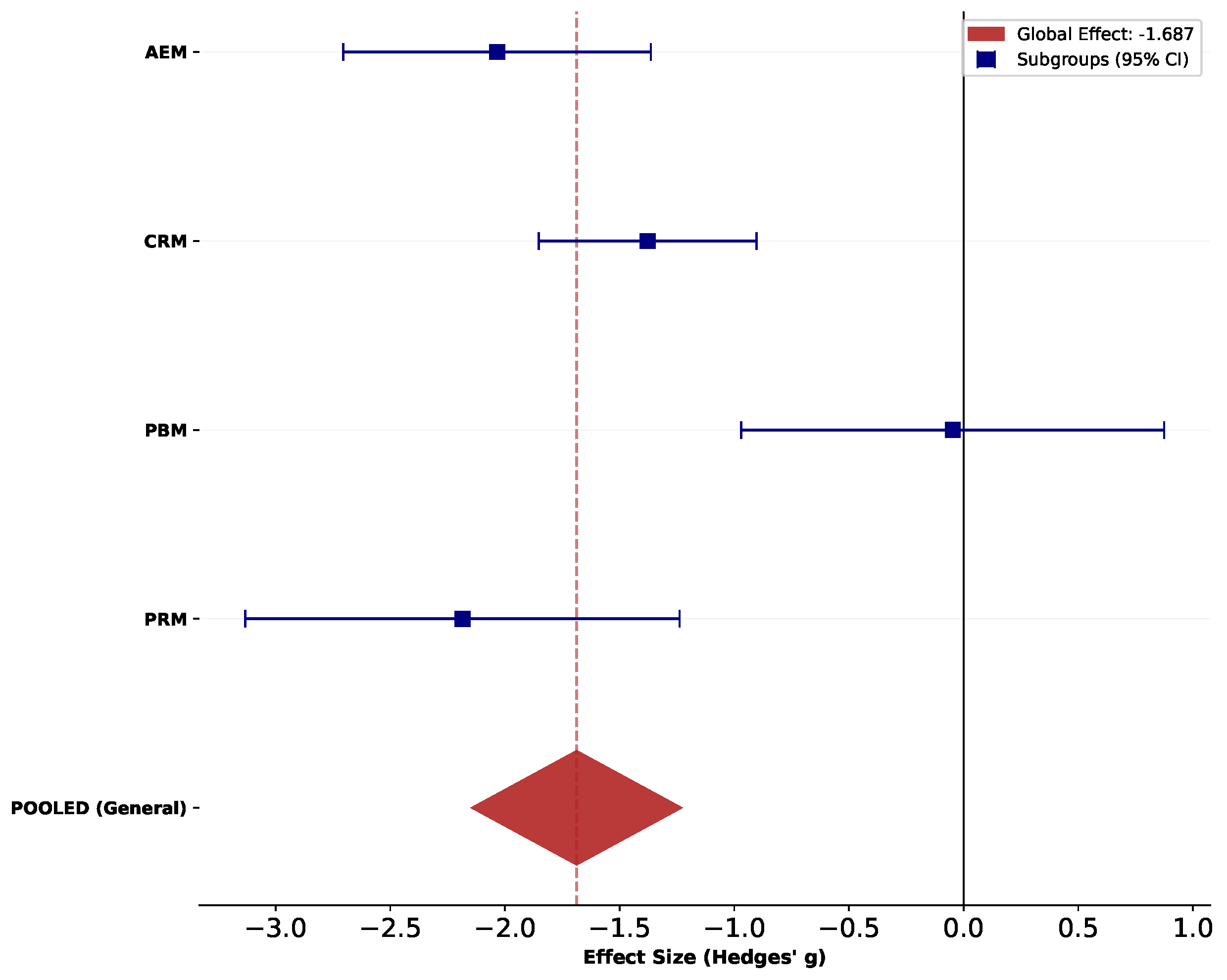
- Absolute Error Metrics (AEM): AEM comprises scale-dependent error measures, which quantify the magnitude of prediction deviations in their original measurement units. The AEM subgroup () produced a large pooled effect (, 95% CI ), indicating substantial reductions in absolute forecasting error relative to the corresponding baselines. However, the wide prediction interval and high heterogeneity suggest considerable between-study variability. Despite this variability, the large Fail-Safe N supports the overall robustness of the observed effect.
- Relative Performance Metrics (PRM): PRM includes normalized error measures, which express prediction errors relative to a reference quantity, thereby facilitating comparisons across datasets with different scales. PRM () showed the largest pooled effect among all subgroups (, 95% CI ). Although statistically robust according to the fail-safe analysis, the broad prediction interval indicates that the magnitude of improvement may vary across different forecasting scenarios.
- Correlation Metrics (CRM): CRM consists of association-based measures, which evaluate the degree of agreement between predicted and observed values. CRM () yielded a moderate-to-large pooled effect (, 95% CI ) with the smallest between-study variance (). Moreover, its prediction interval remained entirely below zero, suggesting the most consistent performance improvement among the evaluated metric families.
- Probability-Based Metrics (PBM): PBM encompasses probabilistic evaluation measures, which quantify predictive uncertainty by evaluating interval coverage, precision, and related interval-based characteristics. PBM () presented a pooled effect close to zero (, 95% CI ), with a prediction interval spanning both positive and negative values. Together with a Fail-Safe N of zero, these results indicate limited evidence for a consistent improvement when probabilistic evaluation metrics are considered.
Figure 6.
Forest Plot General by Metric Families.
3.3.3. Engineering Implications for Wind Farm Development
Taken together, these results indicate that metric family represents an important source of variability in the interpretation of reported forecasting improvements, with direct implications for applied wind energy contexts. Each metric family reflects a distinct decision objective: Absolute Error Metrics (AEM) quantify deviations in physical units and directly support operational forecasting and grid balancing; Relative Performance Metrics (PRM) provide scale-independent measures relevant for cross-site comparisons; Correlation Metrics (CRM) evaluate temporal consistency and pattern reproduction, which are important for short-term dispatch alignment; and Probability-Based Metrics (PBM) characterize uncertainty representation and risk sensitivity, supporting reliability assessment under stochastic wind conditions. Therefore, the selected evaluation framework determines which aspects of forecasting performance are emphasized and influences the interpretation of comparative model results.
From a comparative perspective, AEM exhibits a strong and robust negative pooled effect, representing the most consistent evidence of performance differences across the analyzed studies. However, other metric families also provide relevant information: PRM presents the largest pooled effect among the evaluated metric groups, with robust Fail-safe support, although its prediction interval indicates considerable uncertainty regarding future applications. CRM shows a moderate-to-large negative effect with comparatively lower dispersion and robust statistical support, suggesting that correlation-based criteria capture systematic differences between forecasting approaches. In contrast, PBM exhibits substantially different behavior, with a near-zero pooled effect, broad uncertainty intervals, and limited robustness, indicating greater variability associated with probabilistic calibration procedures and evaluation protocols.
Consequently, differences observed between classical and advanced architectures should not be interpreted as resulting exclusively from model design. Instead, the magnitude and stability of reported improvements appear to depend on the interaction between architectural category, evaluation metric, and study characteristics, which jointly contribute to the observed heterogeneity across forecasting studies.
3.3.4. Methodological Approach to Model Parsimony
An initial Subgroup Combination Analysis (Table 10) evaluates the explanatory contribution of alternative moderator configurations through the Analog variance-reduction criterion. Among the evaluated moderator structures:
- Metric Type alone: Accounts for 9.13% of the estimated between-study heterogeneity, capturing a modest portion of performance dispersion arising from error-metric selection.
- Control Family alone: Explains only 1.70% of the baseline between-study variance, indicating limited explanatory contribution. Control models were aggregated into six conceptually coherent methodological families because most individual control comparator architectures were represented by only one or two effect sizes, providing insufficient replication to estimate model-specific moderator effects. The resulting families comprised Persistence/Reference Ground-Truth (), Physical/NWP Models (), Classical Statistical Models (), Artificial Intelligence-based Models (), Hybrid Physical–AI Models (), and Engineering/Operational Controls (). For illustration, the AI-based family encompassed representative control comparator architectures such as LSTM, GRU, RF or ConvLSTM, whereas the Physical/NWP family included diverse numerical weather prediction frameworks, including WRF variants, NEWA, among others.
- Metric Type + Control Family: Jointly explain 18.15% of the between-study variance, indicating that metric selection and comparator characteristics together capture an expanded proportion of the observed heterogeneity.
- Metric Type + Sample Size: Further improves explanatory performance by accounting for 34.88% of the baseline variance, highlighting the critical moderating role of dataset scale.
- Metric Type + Control Family + Sample Size: Maximizes variance reduction by explaining 40.47% of the total heterogeneity, yielding the lowest residual heterogeneity ().
Although the Metric + Control + Sample Size model provides the highest explanatory power, its higher complexity results in an increased AIC (200.4425) compared with the more parsimonious Metric + Sample Size specification (AIC = 196.5845, ), highlighting a trade-off between variance explanation and model parsimony.
- Model Architecture and Baseline: The mixed-effects meta-regression (see Table 11) simultaneously evaluates metric classification, comparator family, and sample scale. The intercept (, ) represents the baseline configuration: Absolute Error Metrics (AEM) and the Engineering/Operational control family.
- Sample-Size Impact: Sample scale is an important driver of effect-size variation. Massive datasets exhibit a highly significant negative effect (, ), indicating that large observation volumes yield lower effect estimates relative to the baseline.
- Metric and Comparator Moderation: Holding scale and comparator type constant, none of the alternative metric types (PRM, PBM, CRM) show statistically significant departures from the AEM reference. Among comparator families, Physical/NWP models display a marginally significant negative association (, ). The remaining control groups (AI, Statistical, Persistence/Reference, and Hybrid) do not significantly differ from the Engineering baseline at the standard level.
- Model Fit and Variance Explanation: The full multivariable meta-regression model accounts for a substantial portion of the between-study variance (), reducing residual heterogeneity from a global in the unconditional model to a residual . The omnibus test confirms the strong overall explanatory power of these combined moderators (, ).
- Robustness Note: Sample scale remains the most robust predictor under multivariable control. As demonstrated in Table 10, while the full model explains the most variance, the simpler “Metric + Sample Size” model provides the optimal balance of fit and parsimony.
- Subgroup Synthesis by Control Family:Table 12 isolates the pooled effect sizes (g) by comparator type. Classical Statistical models () and Physical/NWP models () yield the most substantial negative pooled estimates, closely followed by AI-based controls (). Conversely, Engineering/Operational baselines show virtually no aggregate difference (). Across all subgroups, extreme heterogeneity persists.

Table 11.
Mixed-effects meta-regression.
| Moderator | SE | p | Sig. | |
|---|---|---|---|---|
| Intercept (Ref: AEM Metric, Engineering Control) | 0.4898 | 1.1436 | 0.6708 | ns |
| Massive dataset | -2.6660 | 0.7375 | 0.0008 | *** |
| Metric: PRM | -0.7614 | 0.8682 | 0.3859 | ns |
| Metric: PBM | 0.8764 | 0.8367 | 0.3014 | ns |
| Metric: CRM | 0.1877 | 0.8529 | 0.8269 | ns |
| Comparator: AI | -1.3333 | 1.1943 | 0.2711 | ns |
| Comparator: Physical | -2.2723 | 1.2240 | 0.0709 | . |
| Comparator: Statistical | -2.2277 | 1.3386 | 0.1041 | ns |
| Comparator: Persistence/Reference | -2.0211 | 1.4774 | 0.1792 | ns |
| Comparator: Hybrid | -0.0662 | 1.6898 | 0.9689 | ns |
Global : 2.5102 | Residual : 1.4943 | Analog : 40.47%; (). Significance codes: *** , . , ns: not significant.
Table 12.
Subgroup meta-analysis synthesis by control family.
| Comparison Family | k | g | 95% CI | 95% PI | |
|---|---|---|---|---|---|
| Persistence/ Reference | 4 | -1.437 | [-2.835, -0.040] | [-6.509, 3.634] | 99.9% |
| Physical/ NWP | 15 | -1.890 | [-2.565, -1.215] | [-4.842, 1.062] | 99.9% |
| Classical Statistical | 7 | -1.940 | [-3.671, -0.209] | [-8.052, 4.172] | 99.9% |
| Artificial Intelligence (AI)-based | 18 | -1.847 | [-2.515, -1.178] | [-4.979, 1.286] | 99.9% |
| Hybrid Physical-AI | 2 | -0.852 | [-2.326, 0.622] | N/A | 99.9% |
| Engineering/ Operational | 3 | -0.018 | [-2.978, 2.942] | [-13.015, 12.979] | 99.9% |
Given that sample size emerged as an strong moderator in the subgroup combination analysis, an additional sensitivity analysis was performed to determine whether studies with exceptionally large datasets disproportionately influenced the pooled estimates. Specifically, the complete dataset was compared with a restricted analysis excluding studies classified as “Massive” ( observations) (see Table 13).
- Effect Size Sensitivity: The full dataset yields a pooled effect size of , whereas excluding massive datasets () reduces the estimated effect to , indicating that large-scale datasets contribute to the magnitude of the synthesized effects.
- Heterogeneity Sensitivity: Removing massive datasets reduces total heterogeneity from to . This subgroup comparison provides complementary sensitivity evidence, while the formal contribution of sample scale is evaluated through the mixed-effects meta-regression model (see Table 11).
- Prediction Uncertainty: The full dataset presents a wider prediction interval () compared with the non-massive subgroup (), indicating increased variability when massive sample-size configurations are included. However, both intervals cross zero, suggesting that the magnitude of improvements remains dependent on study-specific conditions.
The forest plots (Figure 7 and Figure 8) illustrate the interaction between architectural category and evaluation metric, revealing substantial variability in the magnitude and stability of reported effects. Absolute Error Metrics (AEM) show consistent negative effects across configurations, with significant improvements observed for both Advanced (AI) and Classic (Physical) models, while Hybrid configurations present greater uncertainty.
Correlation Metrics (CRM) generally show consistent negative effects. Advanced (AI) CRM demonstrates a significant reduction (, 95% CI ), while Advanced (Hybrid) CRM presents an even more concentrated estimate (, 95% CI ). Conversely, Classic (Physical) CRM exhibits a highly uncertain estimate (, 95% CI ), suggesting substantial uncertainty associated with this configuration. Overall, correlation-based evaluations appear more stable for advanced forecasting approaches than for classical physical configurations.
Relative Performance Metrics (PRM) present large negative effects but considerable uncertainty. Advanced (Hybrid) PRM shows a statistically significant reduction (, 95% CI ), whereas Advanced (AI) PRM exhibits a highly variable estimate with a very wide confidence interval (, 95% CI ). These results suggest that relative metrics may capture substantial improvements in some applications but remain sensitive to dataset characteristics and evaluation conditions.
Probability-Based Metrics (PBM) display the greatest inconsistency among metric families. Advanced (AI) PBM produces an effect close to zero (, 95% CI ), and Advanced (Hybrid) PBM also shows no significant difference (, 95% CI ). In contrast, Classic (Physical) PBM presents a positive and significant effect (, 95% CI ), indicating that probabilistic evaluation outcomes differ substantially according to forecasting framework and metric implementation.
When studies associated with massive sample sizes are excluded (see Figure 9), the pooled effect decreases in magnitude while remaining statistically significant, indicating that large-scale datasets contribute to stronger observed improvements but do not fully explain the overall effect.
From a decision-oriented perspective, the results indicate that model performance comparisons are strongly influenced by the evaluation framework. Correlation Metrics (CRM) provide the most consistent evidence of improvement for Advanced AI and Hybrid architectures in terms of temporal pattern reproduction, with similar effects observed after excluding massive datasets. Absolute Error Metrics (AEM) highlight substantial error reductions for Classical Physical and Advanced AI models, although improvements vary across architectures. In contrast, Probability-Based Metrics (PBM) do not provide stable differentiation among model classes, while Relative Performance Metrics (PRM) show greater sensitivity to dataset composition and uncertainty. Overall, the relevance of an evaluation metric depends jointly on its conceptual purpose, the forecasting characteristics it emphasizes, and the consistency of the resulting performance differences across model classes.
To complement this decision framework, Table 14 presents representative studies reporting the largest and most precisely estimated effects within each methodological paradigm. These configurations illustrate cases associated with strong observed improvements under specific experimental conditions; however, they should not be interpreted as evidence of model superiority. The substantial between-study variability identified in the meta-analysis indicates that the transferability of these results depends on factors such as dataset characteristics, forecasting horizon, operational requirements, and evaluation criteria.
3.4. Additional Robustness Analyses
To address potential concerns regarding the choice of estimator, the pooled heterogeneity between prediction and target, and the absence of formal pairwise comparisons between architecture categories, three complementary analyses were conducted using the effect sizes and standard errors already reported in the Study Data Appendix (Table A1). In accordance with journal policy on the use of generative artificial intelligence, the authors disclose that these three supplementary analyses (Table 15, Table 16 and Table 17) were computed with the assistance of a generative AI tool (Claude, Anthropic) applied to the effect-size dataset in Table A1; the authors reviewed the computations and take full responsibility for the content of this publication.
Sensitivity to the between-study variance estimator. The global random-effects model (Table 3) was re-estimated using the Paule–Mandel and REML estimators of as alternatives to DerSimonian–Laird, following common recommendations for meta-analyses with extreme heterogeneity ( near 100%), using the 49 extracted effect sizes and standard errors underlying the primary analysis. As shown in Table 15, the pooled point estimate is stable across estimators ( to ), while the Paule–Mandel and REML estimators yield a materially larger than DerSimonian–Laird ( vs. ) and correspondingly wider confidence intervals. This is the expected behavior of DL under extreme heterogeneity and does not alter the sign, magnitude, or statistical significance of the pooled effect; it reinforces the manuscript’s existing caution against over-interpreting the global estimate as a precise quantity, while confirming that the qualitative conclusion is not an artifact of estimator choice.
Subgroup meta-analysis by prediction target. Because the corpus pools Wind Power Output (WPO), Wind Speed Profile (WSP), and Atmospheric Conditions (ATM) as prediction targets with different physical relationships and uncertainty structures, a separate random-effects meta-analysis was run for each target (Table 16). The pooled effect is largest and most precise for WPO, moderate for WSP, and smallest, least precise, and not statistically distinguishable from zero for ATM (). This indicates that pooling across targets is not neutral to the overall result and that conclusions about “forecasting performance” should be read primarily at the level of each target rather than as a single undifferentiated construct.
Pairwise contrasts between architecture families. To formally test whether the pooled effects of Physical, AI, and Hybrid architectures reported in Table 7 are statistically distinguishable from one another, pairwise z-tests were computed between the independently pooled effect sizes of each family (Table 17). Physical and AI models are statistically indistinguishable (); Hybrid models show a significantly smaller pooled effect than Physical models () and a marginally smaller effect than AI models (). This refines the manuscript’s architecture-level narrative: the relevant contrast in this corpus is not “Classical vs. Advanced,” but specifically “Hybrid vs. the rest,” since Physical and AI architectures do not differ significantly from each other.
4. Discussion
The results of this meta-analysis indicate that improvements in wind energy forecasting accuracy in coastal and complex environments cannot be attributed exclusively to forecasting architecture. Instead, observed performance differences emerge from the interaction between model formulation, evaluation metric, sample-scale characteristics, and study-specific conditions. Although the overall random-effects estimate indicates a significant average reduction in forecasting error, the substantial residual heterogeneity demonstrates that this effect should not be interpreted as a universal ranking of forecasting approaches, but rather as an aggregate estimate conditioned by relevant moderators.
Advanced AI and hybrid approaches demonstrate strong improvements in specific configurations, particularly under data-intensive scenarios and selected evaluation frameworks; however, these advantages are not consistently maintained across heterogeneous study conditions. Conversely, classical physical approaches exhibit competitive and, in several comparisons, more stable observed performance, with comparatively consistent effects across evaluation settings. This suggests that classical approaches may represent a reliable baseline when no specific forecasting objective or data advantage is available. Overall, model effectiveness appears to depend on the compatibility between forecasting objectives, data characteristics, and evaluation criteria.
The analysis further demonstrates that evaluation metrics influence the interpretation of model performance. Absolute Error Metrics (AEM) show consistent negative effects across several configurations, supporting their relevance for measuring reductions in forecasting error magnitude. Correlation Metrics (CRM) provide complementary information regarding temporal pattern reproduction and may better capture improvements associated with pattern-learning capabilities. In contrast, Probability-Based Metrics (PBM) display limited differentiation among most approaches, whereas Relative Performance Metrics (PRM) show larger effects but greater uncertainty. These results emphasize that metric selection should be aligned with the intended operational objective rather than treated as a neutral measurement choice.
The hypothesis evaluation indicates that architecture category alone is insufficient to explain the observed variability in forecasting improvements. The mixed-effects comparison between Advanced and Classical approaches did not reveal statistically significant differences (), and therefore the hypothesis of a systematic superiority of Advanced architectures was not supported. However, subgroup analyses reveal that architectural effects are conditional on the evaluation framework. Classical physical models demonstrated particularly strong and consistent effects for deterministic error reduction, with Absolute Error Metrics showing comparable or larger improvements than Advanced configurations, a pattern that remained after excluding the influential large-scale dataset. In contrast, Advanced AI and hybrid approaches exhibited stronger effects in correlation-based assessments, suggesting advantages in reproducing predictive patterns rather than uniformly reducing error magnitude. These architecture–metric differences were descriptive rather than formally tested as interaction effects and should therefore be interpreted cautiously.
The moderator analyses identify dataset scale as the dominant moderator of between-study heterogeneity. While Metric Type and Control Family alone explained only 9.13% and 1.70% of the baseline variance, respectively, combining Metric Type with Sample Size increased the explained heterogeneity to 34.88%. Although the full moderator structure achieved the highest explanatory power (Analog ; reduced from 2.5102 to 1.4943), the more parsimonious Metric Type + Sample Size model provided the better balance between explanatory performance and model complexity. Consistent with these findings, the multivariable meta-regression identified the Massive dataset category ( observations) as the only statistically significant moderator (, ), whereas neither metric type nor comparator family showed significant effects after adjustment. Nevertheless, the remaining residual heterogeneity indicates that forecasting performance continues to depend on application-specific factors beyond those captured by the evaluated moderators.
4.1. Limitations
Several limitations should be considered when interpreting these results. First, although the search strategy and PICO framework were designed to include purely statistical reference models alongside physical models under the Classical category, no eligible study in the final corpus used such a comparator; consequently, the Classical category in this synthesis reflects Pure Physical models only, and no claim in this study should be read as evidence about the relative performance of traditional statistical forecasting methods. Second, effect sizes were reconstructed from reported aggregate performance metrics rather than from raw sample-level distributions; Hedges’ g in this framework is therefore best interpreted as a within-study standardized index of relative performance gain rather than a classical standardized mean difference with sampling-level variance guarantees, a distinction already noted in Section 2 and reiterated here as a structural constraint of the evidence base rather than a computational error. Third, sample size (observation count) was used as the principal proxy for dataset scale; this measure does not fully capture effective information content, since temporal resolution, forecast horizon, spatial coverage, and the degree of temporal dependence can influence the effective sample size independently of raw observation count. Fourth, the Physical and AI architecture families each aggregate methodologically diverse approaches, which may conceal within-family heterogeneity beyond what the Control Family stratification in Table 12 already captures. These limitations do not invalidate the exploratory and descriptive approach adopted throughout this study; they are presented in the interest of transparency, and not as issues that have already been resolved.
Future meta-analytic efforts in computational architectures used for estimating wind-related variables should focus on mapping systems that encompass the full spectrum of assessment practices per study before attempting quantitative grouping. Furthermore, we also consider it relevant that, instead of attempting global syntheses of site characteristics through fragmented sets of metrics, future meta-analyses should concentrate on studies with more defined and specific atmospheric regimes, such as tropical coastal microclimates influenced by the Intertropical Convergence Zone (ITCZ), where environmental parameters and spatial scales can be kept constant to ensure sufficient study density per analytical subgroup.
5. Conclusions
This synthesis of 49 studies indicates that improvements in wind forecasting accuracy in coastal and complex-terrain environments cannot be attributed to forecasting architecture alone. A categorical meta-regression found no statistically significant evidence that Advanced (AI, Hybrid) architectures systematically outperform Classical Physical models (, ); pairwise contrasts further show that Physical and AI pooled effects are statistically indistinguishable, while Hybrid models exhibit a significantly smaller pooled effect. Sample Size (massive vs. non-massive datasets) is the only moderator that reaches statistical significance, and metric family (Absolute Error, Correlation, Probability-Based, Relative Performance) substantially conditions the pattern and consistency of reported improvements. No study meeting the eligibility criteria used a purely statistical reference model, so this synthesis speaks specifically to Physical, AI, and Hybrid forecasting approaches. Given extreme between-study heterogeneity () and a prediction interval crossing zero, the global pooled effect should be read descriptively rather than as confirmatory evidence of a specific magnitude of improvement; the practically informative results are the stratified, moderator, and pairwise analyses reported throughout this study. Classical Physical models remain a reliable, comparatively stable reference approach, while Advanced architectures show descriptive advantages only in specific, non-generalizable settings, particularly correlation-based evaluation of temporal pattern reproduction. Future work should prioritize harmonized extraction of forecast horizon, spatial resolution, and input-variable configuration across a corpus of this size, and should seek out eligible studies using classical statistical reference models to close the gap identified in Section 4.1.
Author Contributions
Conceptualization, M.C.-R. and A.O.-C.; methodology, M.C.-R., A.O.-C. and D.R.-L.; software, M.C.-R. and D.R.-L.; validation, M.C.-R., A.O.-C., C.R.-A. and I.T.-O.; formal analysis, M.C.-R. and D.R.-L.; investigation, M.C.-R., C.R.-A. and I.T.-O.; resources, A.O.-C. and C.R.-A.; data curation, M.C.-R., D.R.-L. and I.T.-O.; writing—original draft preparation, M.C.-R.; writing—review and editing, M.C.-R., A.O.-C., D.R.-L., C.R.-A. and I.T.-O.; visualization, M.C.-R. and D.R.-L.; supervision, A.O.-C. and C.R.-A.; project administration, A.O.-C.; funding acquisition, A.O.-C. and C.R.-A. All authors have read and agreed to the published version of the manuscript.
Funding
This research was funded by the Ministerio de Ciencia, Tecnología e Innovación—Fondo Francisco José de Caldas and the Agencia Nacional de Hidrocarburos (ANH), through the Contrato de Financiamiento de Recuperación Contingente No. 112721-053-2025, within the project “Herramientas tecnológicas y prototipos para caracterizar, identificar y optimizar el potencial eólico en zonas costeras de Colombia” (Project Code 111983).
Institutional Review Board Statement
Not applicable. This study is a meta-analysis of previously published, publicly available literature and did not involve new experiments on humans or animals.
Informed Consent Statement
Not applicable.
Data Availability Statement
The data extracted from the 49 included studies (effect sizes, standard errors, sample-size classification, prediction target, architecture, and metric family) are provided in full in Table A1 (Appendix A) and in the accompanying df1.csv dataset. The pre-registered protocol is available on the Open Science Framework [35].
Acknowledgments
Conflicts of Interest
The authors declare no conflicts of interest.
Abbreviations
The following abbreviations are used in this manuscript:
| AI | Artificial Intelligence |
| ML | Machine Learning |
| DL | DerSimonian–Laird (estimator) / Deep Learning (context-dependent) |
| NWP | Numerical Weather Prediction |
| WRF | Weather Research and Forecasting model |
| LSTM | Long Short-Term Memory (neural network) |
| GRU | Gated Recurrent Unit |
| CNN | Convolutional Neural Network |
| RF | Random Forest |
| PICO | Population, Intervention, Comparison, Outcome |
| PRISMA | Preferred Reporting Items for Systematic Reviews and Meta-Analyses |
| SMD | Standardized Mean Difference |
| CI | Confidence Interval |
| PI | Prediction Interval |
| WPO | Wind Power Output |
| WSP | Wind Speed Profile |
| ATM | Atmospheric Conditions |
| REML | Restricted Maximum Likelihood |
| PM | Paule–Mandel (estimator) |
| AEM | Absolute Error Metrics |
| CRM | Correlation Metrics |
| PBM | Probability-Based Metrics |
| PRM | Relative Performance Metrics |
Appendix A. Study Data Appendix
This appendix presents the detailed data obtained during the data-extraction phase, supporting the analyses presented in Section 2 and Section 3.4.
Appendix A.1. Individual Study Results
Table A1.
Individual study results: effect sizes, standard errors, and subgroup classification ().
| ID | Title | ES | SE | Sample Size | Group | Subgroup |
|---|---|---|---|---|---|---|
| [56] | Assessment of wind and wave energy resources and optimal site selection for joint development near the Shandong Peninsula | non_massive | WSP | Classic(Physical) CRM | ||
| [57] | Enhancement of ANN-based WPF over Complex Terrain | non_massive | WPO | Advanced(Hybrid) PRM | ||
| [58] | Day-ahead wind power forecasting based on feature extraction integrating vertical layer wind characteristics in complex Terrain | non_massive | WPO | Advanced(Hybrid) PRM | ||
| [59] | Power prediction method of the offshore wind farm considering high-dimensional feature selection and physical guidance | non_massive | WPO | Advanced(Hybrid) AEM | ||
| [60] | Enhancing wind field resolution in complex terrain through a knowledge-driven machine learning approach | non_massive | WSP | Advanced(AI) AEM | ||
| [61] | Enhancing spatiotemporal wind power forecasting with meta-learning in data-scarce environments | massive | WPO | Advanced(AI) AEM | ||
| [62] | Enhancing offshore wind Resource assessment through neural network-based HF radar data analysis | non_massive | WSP | Advanced(AI) AEM | ||
| [63] | Estimation of Offshore Wind Speed in the Coastal Region of The Southern State of Bahia | non_massive | WSP | Classic(Physical) PBM | ||
| [64] | A graph neural model for predicting wind speed behavior based on the effect of wind speed point coupling | non_massive | WSP | Advanced(AI) PBM | ||
| [65] | A hybrid WOA-KDE and mixed copula framework for directional wind assessment in complex terrain | non_massive | ATM | Advanced(Hybrid) PBM | ||
| [66] | Atmospheric stability from numerical weather prediction models and microwave radiometer observations for onshore and offshore wind energy applications | non_massive | ATM | Classic(Physical) AEM | ||
| [67] | A new fusion model for enhanced ultra-short-term offshore wind power forecasting | non_massive | WPO | Advanced(Ensemble) PRM | ||
| [68] | Effects of Turbulence Modeling on the Simulation of Wind Flow over Typical Complex Terrains | non_massive | ATM | Classic(Physical) AEM | ||
| [69] | Study on Downscaling Correction of Near-Surface Wind Speed Grid Forecasts in Complex Terrain | massive | WSP | Advanced(Hybrid) PRM | ||
| [70] | Simulating Near-Surface Winds in Europe with the WRF Model: Assessing Parameterization Sensitivity Under Extreme Wind Conditions | non_massive | WSP | Classic(Physical) AEM | ||
| [71] | DBANN: Dual-Branch Attention Neural Networks with hierarchical spatiotemporal-perception for multi-node offshore wind power forecasting | massive | WPO | Advanced(AI) PRM | ||
| [72] | Dynamic coupled Atmosphere-Ocean-Wave modeling for enhanced coastal wind resource assessment | non_massive | WSP | Classic(Physical) AEM | ||
| [73] | Prediction Model of Offshore Wind Power Based on Multi-Level Attention Mechanism and Multi-Source Data Fusion | non_massive | WPO | Advanced(AI) AEM | ||
| [74] | On Predicting Offshore Hub Height Wind Speed and Wind Power Density in the Northeast US Coast Using High-Resolution WRF Model Configurations during Anticyclones Coinciding with Wind Drought | massive | WSP | Classic(Physical) AEM | ||
| [75] | A CFD Model for Spatial Extrapolation of Wind Field over Complex Terrain-Wi.Sp.Ex | non_massive | WSP | Classic(Physical) AEM | ||
| [76] | Prediction for Coastal Wind Speed Based on Improved Variational Mode Decomposition and Recurrent Neural Network | massive | WSP | Advanced(Hybrid) AEM | ||
| [77] | Ultra-Short-Term Wind Power Forecasting in Complex Terrain: A Physics-Based Approach | non_massive | WPO | Classic(Physical) AEM | ||
| [78] | Enhancing coastal wind simulation in the WRF model: Updates in sea surface temperature and roughness length through dynamic boundary conditions | non_massive | WSP | Classic(Physical) AEM | ||
| [79] | Hybrid iForest-DBSCAN for anomaly detection and wind power curve modelling | non_massive | WPO | Advanced(Hybrid) PBM | ||
| [80] | A Novel Security Situation Awareness Method for Offshore Wind Power Networking System Based on Vague-CNN-LSTM Model | non_massive | ATM | Advanced(AI) PBM | ||
| [81] | Investigación sobre la predicción de la generación de energía eólica marina mediante un mecanismo de atención híbrido y memoria a largo plazo bidireccional basado en aprendizaje profundo | non_massive | WPO | Advanced(AI) PRM | ||
| [82] | Understanding Wind Characteristics Over Different Terrains for Wind Turbine Deployment | non_massive | WSP | Classic(Physical) AEM | ||
| [83] | Meteorological Assessment of Vertical Axis Wind Turbine Energy Microgeneration Potentials Across Two Swiss Cities Located in Complex Terrain | non_massive | WSP | Classic(Physical) AEM | ||
| [84] | Optimization Method of Wind Turbine Locations in Complex Terrain Areas Using a Combination of Simulation and Analytical Models | non_massive | WPO | Advanced(Hybrid) AEM | ||
| [85] | Hybrid Intelligent Optimisation for Onshore Wind Farm Forecasting | non_massive | WPO | Advanced(Hybrid) PBM | ||
| [86] | Short-term offshore wind power multi-location multi-modal multi-step prediction model based on Informer (M3STIN) | massive | WPO | Advanced(Hybrid) AEM | ||
| [87] | Short-term offshore wind speed prediction model based on VMD-GDPSO-TCN-BiLSTM | non_massive | WSP | Advanced(Hybrid) CRM | ||
| [88] | Short-term wind power forecasting in complex terrain based on spatiotemporal enhanced deep correction network | massive | WPO | Advanced(AI) AEM | ||
| [89] | Short-term wind power prediction based on multiscale numerical simulation coupled with deep learning | non_massive | WSP | Advanced(Hybrid) AEM | ||
| [90] | A Dynamic Hidden Markov Model with Real-Time Updates for Multi-Risk Meteorological Forecasting in Offshore Wind Power | non_massive | ATM | Advanced(AI) PBM | ||
| [91] | WD-SGformer: high-precision wind power forecasting via dual-attention dynamic spatio-temporal learning | massive | WPO | Advanced(AI) AEM | ||
| [92] | Machine-learning-based estimate of the wind speed over complex terrain using the long short-term memory (LSTM) recurrent neural network | non_massive | WSP | Advanced(AI) CRM | ||
| [93] | Improving wind and power predictions via four-dimensional data assimilation in the WRF model: case study of storms in February 2022 at Belgian offshore wind farms | non_massive | WSP | Classic(Physical) AEM | ||
| [94] | Wind power forecasting based on a machine learning model: considering a coastal wind farm in Zhejiang as an example | massive | WPO | Advanced(AI) AEM | ||
| [95] | Wind Estimation Methods for Nearshore Wind Resource Assessment Using High-Resolution WRF and Coastal Onshore Measurements | non_massive | WSP | Classic(Classic) CRM | ||
| [96] | Improved spatio-temporal offshore wind forecasting with coastal upwelling information | non_massive | WPO | Advanced(Hybrid) AEM | ||
| [97] | Short-term offshore wind speed forecast by seasonal ARIMA - A comparison against GRU and LSTM | non_massive | WSP | Advanced(AI) CRM | ||
| [98] | Forecast Optimization of Wind Speed in the North Coast of the Yucatan Peninsula, Using the Single and Double Exponential Method | non_massive | WSP | Advanced(AI) AEM | ||
| [99] | Deterministic and Probabilistic Wind Power Forecasts by Considering Various Atmospheric Models and Feature Engineering Approaches | massive | WPO | Advanced(Ensemble) PRM | ||
| [100] | Machine learning methods to improve spatial predictions of coastal wind speed profiles and low-level jets using single-level ERA5 data | non_massive | WSP | Advanced(AI) AEM | ||
| [101] | A Deep Learning Model for Improved Wind and Consequent Wave Forecasts | non_massive | WSP | Advanced(AI) AEM | ||
| [102] | EEMD-ConvLSTM: a model for short-term prediction of two-dimensional wind speed in the South China Sea | non_massive | WSP | Advanced(AI) AEM | ||
| [103] | Interpretable machine learning for coastal wind prediction: Integrating SHAP analysis and seasonal trends | non_massive | WSP | Advanced(AI) CRM | ||
| [104] | Improving the Forecasts of Coastal Wind Speeds in Tianjin, China Based on the WRF Model with Machine Learning Algorithms | non_massive | WSP | Advanced(Hybrid) AEM |
Appendix A.2. Publication Bias Analysis
Table A4.
Individual study results and statistical weights for meta-analysis.
| # | ID | ES | CI LL | CI UL | W (%) | # | ID | ES | CI LL | CI UL | W (%) |
|---|---|---|---|---|---|---|---|---|---|---|---|
| 1 | [56] | 2.0400 | 26 | [81] | 2.0400 | ||||||
| 2 | [57] | 2.0400 | 27 | [82] | 2.0400 | ||||||
| 3 | [58] | 2.0400 | 28 | [83] | 2.0400 | ||||||
| 4 | [59] | 2.0400 | 29 | [84] | 2.0400 | ||||||
| 5 | [60] | 2.0400 | 30 | [85] | 2.0400 | ||||||
| 6 | [61] | 2.0400 | 31 | [86] | 2.0400 | ||||||
| 7 | [62] | 2.0400 | 32 | [87] | 2.0400 | ||||||
| 8 | [63] | 2.0400 | 33 | [88] | 2.0400 | ||||||
| 9 | [64] | 2.0400 | 34 | [89] | 2.0400 | ||||||
| 10 | [65] | 2.0400 | 35 | [90] | 2.0400 | ||||||
| 11 | [66] | 2.0400 | 36 | [91] | 2.0400 | ||||||
| 12 | [67] | 2.0400 | 37 | [92] | 2.0400 | ||||||
| 13 | [68] | 2.0400 | 38 | [93] | 2.0300 | ||||||
| 14 | [69] | 2.0400 | 39 | [94] | 2.0400 | ||||||
| 15 | [70] | 2.0400 | 40 | [95] | 2.0400 | ||||||
| 16 | [71] | 2.0400 | 41 | [96] | 2.0400 | ||||||
| 17 | [72] | 2.0400 | 42 | [97] | 1.9800 | ||||||
| 18 | [73] | 2.0400 | 43 | [98] | 2.0400 | ||||||
| 19 | [74] | 2.0400 | 44 | [99] | 2.0400 | ||||||
| 20 | [75] | 2.0400 | 45 | [100] | 2.0400 | ||||||
| 21 | [76] | 2.0400 | 46 | [101] | 2.0400 | ||||||
| 22 | [77] | 2.0400 | 47 | [102] | 2.0400 | ||||||
| 23 | [78] | 2.0400 | 48 | [103] | 2.0400 | ||||||
| 24 | [79] | 2.0400 | 49 | [104] | 2.0400 | ||||||
| 25 | [80] | 2.0400 |
Appendix A.3. Normal Quantile Chart Data
Table A5.
Normal quantile plot data: theoretical vs. sample quantiles.
| # | Study | Normal Q. | Sample Q. (Z) | # | Study | Normal Q. | Sample Q. (Z) |
|---|---|---|---|---|---|---|---|
| 1 | [94] | 26 | [103] | ||||
| 2 | [88] | 27 | [58] | ||||
| 3 | [99] | 28 | [92] | ||||
| 4 | [76] | 29 | [61] | ||||
| 5 | [74] | 30 | [78] | ||||
| 6 | [95] | 31 | [93] | ||||
| 7 | [71] | 32 | [59] | ||||
| 8 | [69] | 33 | [100] | ||||
| 9 | [68] | 34 | [96] | ||||
| 10 | [91] | 35 | [70] | ||||
| 11 | [72] | 36 | [102] | ||||
| 12 | [77] | 37 | [89] | ||||
| 13 | [86] | 38 | [65] | ||||
| 14 | [73] | 39 | [75] | ||||
| 15 | [66] | 40 | [64] | ||||
| 16 | [80] | 41 | [62] | ||||
| 17 | [87] | 42 | [79] | ||||
| 18 | [104] | 43 | [56] | ||||
| 19 | [83] | 44 | [97] | ||||
| 20 | [57] | 45 | [85] | ||||
| 21 | [81] | 46 | [82] | ||||
| 22 | [98] | 47 | [63] | ||||
| 23 | [60] | 48 | [90] | ||||
| 24 | [67] | 49 | [84] | ||||
| 25 | [101] |
References
- Allahyarzadeh, A.; Sharifzadeh, M. Integrated carbon capture and renewable technologies for carbon neutral energy hubs: A network-ready superstructure model. Renew. Energy 2026, 256, 124570. [Google Scholar] [CrossRef]
- Chaaben, N.; Saida, I.; Helali, K. Analyzing the non-linear impact of carbon dioxide emissions on renewable energy in Commonwealth nations. Renew. Sustain. Energy Rev. 2026, 227, 116494. [Google Scholar] [CrossRef]
- Graham, E.; Fulghum, N.; Altieri, y K. Global Electricity Review 2025,” Ember, Londres, Reino Unido, Informe. 2025. Available online: https://ember-energy.org/es/analisis/global-electricity-review-2025/.
- Ember. Global Electricity Review 2024: Trends and Data Analysis. 2024. Available online: https://ember-energy.org/latest-insights/global-electricity-review-2024/global-electricity-trends/.
- Ragab, K. M.; Orhan, M. F. Evaluating conventional and renewable energy systems for green buildings: A case study on energy efficiency and cost optimization. Case Stud. Therm. Eng. 2024, 63, 105233. [Google Scholar] [CrossRef]
- Krarti, M.; Aldubyan, M. Role of energy efficiency and distributed renewable energy in designing carbon neutral residential buildings and communities: Case study of Saudi Arabia. Energy Build. 2021, 250, 111309. [Google Scholar] [CrossRef]
- Siddique, M. A.; Nobanee, H.; Hasan, M. B.; Uddin, G. S.; Hossain, M. N.; Park, y D. How do energy markets react to climate policy uncertainty? Fossil vs. renewable and low-carbon energy assets. Energy Econ. 2022, 114. [Google Scholar] [CrossRef]
- Ferreira, G. W. S.; Reboita, M. S. A New Look into the South America Precipitation Regimes: Observation and Forecast. Atmosphere 2022, 13(no. 6), 873. [Google Scholar] [CrossRef]
- Arias, P. A.; et al. , Hydroclimate of the Andes Part II: Hydroclimate Variability and Sub-Continental Patterns. Front. Earth Sci. 2021, 8, 505467. [Google Scholar] [CrossRef]
- Martinez, J. A.; et al. Recent progress in atmospheric modeling over the Andes – part I: review of atmospheric processes. Review 2024. [Google Scholar] [CrossRef]
- Arias, P. A.; et al. How well CMIP6 models simulate key boundary conditions affecting South American climate? Insights for regional modeling efforts. Clim. Dyn. 63, 231, 2025. [CrossRef]
- Byrne, H.; Seager, R.; Smerdon, J. E. CMIP6 models cannot capture long-term forced changes in the tropical Pacific sea surface temperature gradient Art. no. 142. d stratification in river estuaries: a case study of the Magdalena River, Colombia,” Catena. Nat. Commun. 2026, 17. [Google Scholar] [CrossRef] [PubMed]
- Torres-Bejarano, F. M.; Torregroza-Espinosa, A. C.; Restrepo, J. C. Modeling sediment transport and salt stratification in river estuaries: A case study of the Magdalena River, Colombia. Catena 248, 109589. [CrossRef]
- Liu, Y.; Chen, D.; Yi, Q.; Li, S. Wind profiles and wave spectra for potential wind farms in South China Sea. Part I: Wind speed profile model. Energies 2017, 10, 125. [Google Scholar] [CrossRef]
- Naranjo-Vesga, J.; et al. , The Guajira contourite depositional system along the northern Colombian Caribbean convergent margin. Mar. Pet. Geol. 2025, 182, 107556. [Google Scholar] [CrossRef]
- Karpatne, A.; Atluri, G.; Faghmous, J. H.; Steinbach, M.; Banerjee, A.; Ganguly, A.; Shekhar, S.; Samatova, N.; Kumar, V. Theory-Guided Data Science: A New Paradigm for Scientific Discovery from Data. IEEE Trans. Knowl. Data Eng. 2017, 29(no. 10), 2318–2331. [Google Scholar] [CrossRef]
- Naranjo-Vesga, J.; Mantilla, O.; Rincon-Martinez, D.; Rodriguez-Rubio, E.; Ortiz-Karpf, A.; Winter, C.; Rojas-Agramonte, Y. The Guajira contourite depositional system along the northern Colombian Caribbean convergent margin. Mar. Pet. Geol. 2025, 182, 107556. [Google Scholar] [CrossRef]
- Kashinath, K.; et al. Physics-informed machine learning: case studies for weather and climate modelling. Philos. Trans. R. Soc. A 2021, 379, 20200093. [Google Scholar] [CrossRef] [PubMed]
- Piotrowski, P.; Rutyna, I.; Baczyński, D.; Kopyt, M. Evaluation metrics for wind power forecasts: A comprehensive review and statistical analysis of errors. Energies 2022, 15, 9657. [Google Scholar] [CrossRef]
- Haq, I.; et al. Machine learning approaches for wind power forecasting: a comprehensive review. Discov. Appl. Sci. 2025, 7, 1139. [Google Scholar] [CrossRef]
- Prema, V.; Bhaskar, M. S. Critical review of data, models and performance metrics for wind and solar power forecast. IEEE Access 2022, 10, 667–688. [Google Scholar] [CrossRef]
- Valdivia-Bautista, S. M. Artificial Intelligence in wind speed forecasting: A review. Energies 2023, 16(no. 5), Art. no. 2457. [Google Scholar] [CrossRef]
- Kwiliński, A.; Lyulyov, O.; Pimonenko, T.; et al. Renewable power systems: A comprehensive meta-analysis. Energies 2024, 17(no. 16, Art. no. 3989). [Google Scholar] [CrossRef]
- Cryer, J. D.; Chan, K.-S. Time Series Analysis: With Applications in R. In New York, NY: Springer, 2nd ed.; 2008. [Google Scholar] [CrossRef]
- McCabe, E. J.; Freedman, J. M. Quantifying the uncertainty in the weather research and forecasting model under sea breeze and low-level jet conditions in the New York Bight: Importance to offshore wind energy. Weather Forecast. 2025, 40(no. 3), 425–450. [Google Scholar] [CrossRef]
- Balasubramanian, K.; Thanikanti, S. B.; Subramaniam, U.; Sudhakar, N.; Sichilalu, S. A novel review on optimization techniques used in wind farm modelling. Renew. Energy Focus 2020, 35, 84–96. [Google Scholar] [CrossRef]
- Lee, S.; Almomani, M. H.; Alomari, S. A.; et al. A novel deep learning framework with artificial protozoa optimization-based adaptive environmental response for wind power prediction. Sci. Rep. 2025, 15, Art.(no. 18746). [Google Scholar] [CrossRef] [PubMed]
- Mo, S.; Wang, H.; Liu, Q. Powerformer: A temporal-based transformer model for wind power forecasting. Energy Rep. 2024, 11(3), 736–744. [Google Scholar] [CrossRef]
- Bui, H.; Bakhoday-Paskyabi, M.; Mohammadpour-Penchah, M. Implementation of a Simple Actuator Disk for Large-Eddy Simulation in the Weather Research and Forecasting Model (WRF-SADLES v1.2) for wind turbine wake simulation. Geosci. Model Dev. 2024, 17(10), 4447–4465. [Google Scholar] [CrossRef]
- Larsén, X. G.; Fischereit, J. A case study of wind farm effects using two wake parameterizations in the Weather Research and Forecasting (WRF) model (V3.7.1) in the presence of low-level jets. Geosci. Model Dev. 2021, 14(6), 3141–3158. [Google Scholar] [CrossRef]
- Fernández-González, S.; Martín, M. L.; García-Ortega, E.; Merino, A.; Lorenzana, J.; Sánchez, J. L.; Valero, F.; Rodrigo, J. S. Sensitivity Analysis of the WRF Model: Wind-Resource Assessment for Complex Terrain. J. Appl. Meteor. Climatol. 2018, 57(3), 733–753. [Google Scholar] [CrossRef]
- Giannakopoulou, E.-M.; Nhili, R. WRF Model Methodology for Offshore Wind Energy Applications. Adv. Meteorol. 2014, Art. no. 319819. [Google Scholar] [CrossRef]
- Sandeepan, B. S.; Panchang, V. G.; Nayak, S.; Kumar, K. K.; Kaihatu, J. M. Performance of the WRF Model for Surface Wind Prediction around Qatar. J. Atmos. Ocean. Technol. 2018, 35(3), 575–592. [Google Scholar] [CrossRef]
- Schütt, M. Wind turbines and property values: a meta-regression analysis. Environ. Resour. Econ. 2024, 87, 1–43. [Google Scholar] [CrossRef]
- Restrepo, D.; Carrillo, M. Protocol for the review and meta-analysis of the accuracy of Advanced Methods (AI, Ensemble and Hybrid) versus Classical Methods (Pure Physical and Statistical) for estimating wind power at onshore and offshore sites influenced by coastal or trade wind dynamics. OSF 2025. [Google Scholar] [CrossRef]
- Westgate, M. J. revtools: An R package to support article screening for evidence synthesis. Res. Synth. Methods 2019, 10(no. 4), 606–614. [Google Scholar] [CrossRef] [PubMed]
- van Rhee, H. J.; Suurmond, R.; Hak, T. User manual for Meta-Essentials: Workbooks for meta-analysis. Erasmus Research Institute of Management: Rotterdam, The Netherlands, 2015. Available online: https://repub.eur.nl/pub/78635/User-manual-1.3.pdf.
- Suurmond, R.; van Rhee, H.; Hak, T. Introduction, comparison, and validation of Meta-Essentials: A free and simple tool for meta-analysis. Res. Synth. Methods 2017, 8(no. 4), 537–553. [Google Scholar] [CrossRef] [PubMed]
- Hak, T.; van Rhee, H. J.; Suurmond, R. How to interpret results of meta-analysis,” Erasmus Rotterdam Institute of Management, Rotterdam, The Netherlands. 2016. Available online: https://repub.eur.nl/pub/80102/How-to-interpret-results-of-meta-analysis-1.3.pdf.
- Hansen, C.; Steinmetz, H.; Block, J. How to conduct a meta-analysis in eight steps: a practical guide. Manag. Rev. Q. 2022, 72(no. 1), 1–19. [Google Scholar] [CrossRef]
- Schmidt, F. L.; Hunter, J. E. Comparison of three meta-analysis methods revisited: An analysis of Johnson, Mullen, and Salas (1995). J. Appl. Psychol. 1999, 84(no. 1), 144–148. [Google Scholar] [CrossRef]
- Hedges, L. V.; Gurevitch, J.; Curtis, P. S. The meta-analysis of response ratios in experimental ecology. Ecology 1999, 80(4), 1150–1156. [Google Scholar] [CrossRef] [PubMed]
- Hedges, L. V. Distribution theory for Glass’s estimator of effect size and related estimators. J. Educ. Behav. Stat. 1981, 6(no. 2), 107–128. [Google Scholar] [CrossRef]
- Austin, P. C. Absolute risk reductions, relative risks, relative risk reductions, and numbers needed to treat can be obtained from a logistic regression model. J. Clin. Epidemiol. 2010, 63(no. 1), 2–6. [Google Scholar] [CrossRef] [PubMed]
- Andrade, C. Understanding relative risk, odds ratio, and related terms: as simple as it can get. J. Clin. Psychiatry 2015, 76(no. 7), e857–e861. [Google Scholar] [CrossRef] [PubMed]
- Borenstein, M.; Hedges, L. V.; Higgins, J. P.; Rothstein, H. R. Introduction to Meta-Analysis; Capítulo sobre Effect Sizes based on Ratios; John Wiley & Sons, 2009. [Google Scholar]
- Sánchez-Meca, J.; Marín-Martínez, F.; Chacón-Moscoso, S. Effect-size indices for dichotomized outcomes in meta-analysis. Psychol. Methods 2003, 8(no. 4), 448–467. [Google Scholar] [CrossRef] [PubMed]
- Cohen, J. Statistical Power Analysis for the Behavioral Sciences, 2nd ed.; Erlbaum: New York, NY, USA, 1998. [Google Scholar]
- Kyriakou, S.; Kosmidis, I.; Sartori, N. Median bias reduction in random-effects meta-analysis and meta-regression. Stat. Methods Med. Res. 2019, 28(no. 6), 1622–1636. [Google Scholar] [CrossRef] [PubMed]
- Raudenbush, S. W.; Bryk, A. S. Hierarchical Linear Models: Applications and Data Analysis Methods, 2nd ed.; Sage Publications: Newbury Park, CA, USA, 2002. [Google Scholar]
- Haddaway, N. R.; Page, M. J.; Pritchard, C. C.; McGuinness, L. A. PRISMA2020: An R package and Shiny app for producing PRISMA 2020-compliant flow diagrams, with interactivity for optimised digital transparency and Open Synthesis. Campbell Syst. Rev. 2022, 18(no. 2), e1230. [Google Scholar] [CrossRef] [PubMed]
- Hedges, L. V.; Rosenthal, R.; Cooper, H. Parametric measures of effect size. In The Handbook of Research Synthesis; Russell Sage Foundation: New York, NY, USA, 1994; pp. 231–244. [Google Scholar] [CrossRef]
- Egger, M.; Davey Smith, G.; Schneider, M.; Minder, C. Bias in meta-analysis detected by a simple, graphical test. Brit. Med. J. 1997, 315(no. 7109), 629–634. [Google Scholar] [CrossRef] [PubMed]
- Rosenthal, R. The `file-drawer’ problem and tolerance for null results. Psychol. Bull. 1979, 86(no. 3), 638–641. [Google Scholar] [CrossRef]
- Begg, C. B.; Mazumdar, M. Operating characteristics of a rank correlation test for publication bias. Biometrics 1994, 50(no. 4), 1088–1101. [Google Scholar] [CrossRef]
- Cao, F.; Li, Y.; Ning, D.; Shi, H.; Han, Z. Assessment of wind and wave energy resources and optimal site selection for joint development near the Shandong Peninsula. Ocean Eng. [CrossRef]
- Kim, J.; Shin, H.; Lee, K.; Hong, J. Enhancement of ANN-based wind power forecasting by modification of surface roughness parameterization over complex terrain. J. Environ. Manag. [CrossRef] [PubMed]
- Lee, K.; Park, B.; Kim, J.; Hong, J. Day-ahead wind power forecasting based on feature extraction integrating vertical layer wind characteristics in complex terrain. Energy. [CrossRef]
- Hua, H.; Wang, Y.; Han, K.; Liu, C.; Zhang, K.; Chen, P.; Bao, Y. Power prediction method of the offshore wind farm considering high-dimensional feature selection and physical guidance. Electr. Power Syst. Res. [CrossRef]
- Wold, J. W.; Stadtmann, F.; Rasheed, A.; Tabib, M.; San, O. Enhancing wind field resolution in complex terrain through a knowledge-driven machine learning approach. Eng. Appl. Artif. Intell. [CrossRef]
- Wang, R.; Wu, J.; Cheng, X.; Liu, X.; Qiu, H. Enhancing spatiotemporal wind power forecasting with meta-learning in data-scarce environments. Eng. Appl. Artif. Intell. [CrossRef]
- Martzikos, N.; Craven, M.; Walker, D.; Conley, D. Enhancing offshore wind Resource assessment through neural network-based HF radar data analysis. Renew. Energy. [CrossRef]
- Fernandes, G. C.; Lemos, A. T.; Vidal, D. B.; Torres, E. A. Estimation of Offshore Wind Speed in the Coastal Region of The Southern State of Bahia. Rev. Bras. De Geogr. Fis. [CrossRef]
- Xiaoxun, Z.; Huan, X.; Lin, Z.; Yuxuan, L.; Xiaoxia, G.; Haiqiang, W. A graph neural model for predicting wind speed behavior based on the effect of wind speed point coupling. Energy. [CrossRef]
- Wang, W.; Chen, F.; Li, Y.; Weng, L. A hybrid WOA-KDE and mixed copula framework for directional wind assessment in complex terrain. Sustain. Energy Technol. Assess. [CrossRef]
- Cimini, D.; et al. Atmospheric stability from numerical weather prediction models and microwave radiometer observations for onshore and offshore wind energy applications. Atmos. Meas. Tech. 2025, 18(no. 4), 2041–2059. [Google Scholar] [CrossRef]
- Wang, Q.; Xu, F.; He, J.; Luo, K.; Fan, J. A new fusion model for enhanced ultra-short- term offshore wind power forecasting. Renew. Energy. [CrossRef]
- Ma, G.; Tian, L.; Song, Y.; Zhao, N. Effects of Turbulence Modeling on the Simulation of Wind Flow over Typical Complex Terrains. Appl. Sci. 2024, 14(no. 23), 11438. [Google Scholar] [CrossRef]
- Liu, X.; Li, Z.; Shen, Y. Study on Downscaling Correction of Near-Surface Wind Speed Grid Forecasts in Complex Terrain. Atmosphere 2024, 15(no. 9), 1090. [Google Scholar] [CrossRef]
- Lee, M.; Oh, D.; Kim, J. Y.; Kim, C. K. Simulating Near-Surface Winds in Europe with the WRF Model: Assessing Parameterization Sensitivity Under Extreme Wind Conditions. Atmosphere 16(no. 6), 665, 2025. [CrossRef]
- Hu, D.; He, F.; Fan, W.; Feng, W. DBANN: Dual-Branch Attention Neural Networks with hierarchical spatiotemporal-perception for multi-node offshore wind power forecasting. Energy. [CrossRef]
- Fang, F.; Zhu, Y.; Zhang, X.; Niu, Y. Dynamic coupled Atmosphere–Ocean–Wave modeling for enhanced coastal wind resource assessment. Renew. Energy. [CrossRef]
- Xu, Y.; Lin, Y.; Li, S.; Gao, X. Prediction Model of Offshore Wind Power Based on Multi-Level Attention Mechanism and Multi-Source Data Fusion. Electronics 14(no. 16), 3183, 2025. [CrossRef]
- Zaman, T.; Juliano, T. W.; Hawbecker, P.; Astitha, M. On Predicting Offshore Hub Height Wind Speed and Wind Power Density in the Northeast US Coast Using High-Resolution WRF Model Configurations during Anticyclones Coinciding with Wind Drought. Energies 2024, 17(no. 11), 2618. [Google Scholar] [CrossRef]
- Michos, D.; Catthoor, F.; Foussekis, D. A CFD Model for Spatial Extrapolation of Wind Field over Complex Terrain—Wi.Sp.Ex. Energies 2024, 17(no. 16), 4139. [Google Scholar] [CrossRef]
- Du, M.; Zhang, Z.; Ji, C. Prediction for Coastal Wind Speed Based on Improved Variational Mode Decomposition and Recurrent Neural Network. Energies 18(no. 3), 542, 2025. [CrossRef]
- Michos, D.; Catthoor, F.; Foussekis, D.; Kazantzidis, A. Ultra-Short-Term Wind Power Forecasting in Complex Terrain. Energies 2024, 17(no. 21), 5493. [Google Scholar] [CrossRef]
- Wu, C.; Wang, N.; Zhao, Y.; Dong, X.; Huang, W. Enhancing coastal wind simulation in the WRF model: Updates in sea surface temperature and roughness length through dynamic boundary conditions. Dyn. Atmos. Ocean. [CrossRef]
- Mehmood, Z.; Wang, Z. Hybrid iForest-DBSCAN for anomaly detection and wind power curve modelling. Expert Syst. Appl. [CrossRef]
- Tian, S.; Lu, Y.; Zhu, F.; Fan, H.; Yang, X.; Su, X. A Novel Security Situation Awareness Method for Offshore Wind Power Networking System Based on Vague-CNN-LSTM Model, IET Gener. Transm. Distrib. [CrossRef]
- Zhang, Y.; Ma, Y.; Fang, H.; Wang, H. Investigation on forecast of offshore wind power generation hybrid attention mechanism and bi- directional long short-term memory based on deep learning. Ocean Coast. Manag. [CrossRef]
- Kumar, R.; Rutgersson, A.; Asim, M.; Routray, A. Understanding Wind Characteristics Over Different Terrains for Wind Turbine Deployment. Meteorol. Appl. [CrossRef]
- Aldo, B.; Gabriele, M. Meteorological Assessment of Vertical Axis Wind Turbine Energy Microgeneration Potentials Across Two Swiss Cities Located in Complex Terrain. Sustain. Energy Technol. Assess. 2025. [Google Scholar] [CrossRef]
- Thin, D. V.; Sang, L. Q.; Duc, N. H. Optimization Method of Wind Turbine Locations in Complex Terrain Areas Using a Combination of Simulation and Analytical Models. IEEE Access. [CrossRef]
- Gwabavu, M.; Bansal, R. C.; Bryce, A. Hybrid Intelligent Optimisation for Onshore Wind Farm Forecasting. J. Open Innov. Technol. Mark. Complex. [CrossRef]
- Wang, Z.; Wang, C.; Chen, L.; Yu, M.; Yuan, W. Short-term offshore wind power multi-location multi-modal multi-step prediction model based on Informer (M3STIN). Energy. [CrossRef]
- Chen, G.; et al. Short-term offshore wind speed prediction model based on VMD-GDPSO-TCN-BiLSTM. Ocean Eng. [CrossRef]
- Zhang, Y.; et al. Short-term wind power forecasting in complex terrain based on spatiotemporal enhanced deep correction network. Renew. Energy. [CrossRef]
- Li, T.; et al. Short-term wind power prediction based on multiscale numerical simulation coupled with deep learning. Renew. Energy. [CrossRef]
- Yang, R.; Tang, J.; Saga, R.; Ma, Z. A Dynamic Hidden Markov Model with Real-Time Updates for Multi-Risk Meteorological Forecasting in Offshore Wind Power. Sustainability 2025, 17(no. 8), 3606. [Google Scholar] [CrossRef]
- Yang, Y.; Fan, S.; Liu, Z.; Yu, Z. WD-SGformer: high-precision wind power forecasting via dual-attention dynamic spatio- temporal learning. Energy. [CrossRef]
- Beu, C. M. L.; Landulfo, E. Machine-learning-based estimate of the wind speed over complex terrain using the long short-term memory (LSTM) recurrent neural network. Wind Energy Sci. 2024, 9(no. 5), 1431–1447. [Google Scholar] [CrossRef]
- Ivanova, T.; et al. Improving wind and power predictions via four-dimensional data assimilation in the WRF model: case study of storms in February 2022 at Belgian offshore wind farms. Wind Energy Sci. 2025, 10(no. 1), 245–263. [Google Scholar] [CrossRef]
- Gu, G.; et al. Wind power forecasting based on a machine learning model: considering a coastal wind farm in Zhejiang as an example. Int. J. Green Energy. [CrossRef]
- Maruo, T.; Ohsawa, T. Wind Estimation Methods for Nearshore Wind Resource Assessment Using High-Resolution WRF and Coastal Onshore Measurements. Wind 5(no. 3), 17, 2025. [CrossRef]
- Ye, F.; Miles, T.; Ezzat, A. A. Improved spatio-temporal offshore wind forecasting with coastal upwelling information. Appl. Energy. [CrossRef]
- Liu, X.; Lin, Z.; Feng, Z. Short-term offshore wind speed forecast by seasonal ARIMA - A comparison against GRU and LSTM. Energy 2021, 237, 120492. [Google Scholar] [CrossRef]
- Pérez-Albornoz, C.; Hernández-Gómez, Á.; Ramirez, V.; Guilbert, D. Forecast Optimization of Wind Speed in the North Coast of the Yucatan Peninsula, Using the Single and Double Exponential Method. Clean Technol. 2023, 5(no. 2), 37. [Google Scholar] [CrossRef]
- Wu, Y. K.; Huang, C. L.; Wu, S. H.; Hong, J. S.; Chang, H. L. Deterministic and Probabilistic Wind Power Forecasts by Considering Various Atmospheric Models and Feature Engineering Approaches. IEEE Trans. Ind. Appl. 2023, 59(no. 2), 1655–1667. [Google Scholar] [CrossRef]
- Hallgren, C.; et al. Machine learning methods to improve spatial predictions of coastal wind speed profiles and low-level jets using single-level ERA5 data. Wind Energy Sci. 2024, 9(no. 3), 821–838. [Google Scholar] [CrossRef]
- Yevnin, Y.; Toledo, Y. A Deep Learning Model for Improved Wind and Consequent Wave Forecasts. J. Phys. Oceanogr. 2022, 52(no. 12), 2977–2993. [Google Scholar] [CrossRef]
- Sun, H.; et al. EEMD-ConvLSTM: a model for short-term prediction of two-dimensional wind speed in the South China Sea. Artif. Intell. Rev. 2024, 57(no. 3), 50420. [Google Scholar] [CrossRef]
- Durap, A. Interpretable machine learning for coastal wind prediction: Integrating SHAP analysis and seasonal trends. J. Oper. Res. Soc. [CrossRef]
- Zhang, W.; et al. Improving the forecasts of coastal wind speeds in Tianjin, China based on the WRF model with machine learning algorithms. J. Meteorol. Res. 2024, 38(no. 3), 570–585. [Google Scholar] [CrossRef]
Figure 1.
Overlap Scopus vs Web of Science.
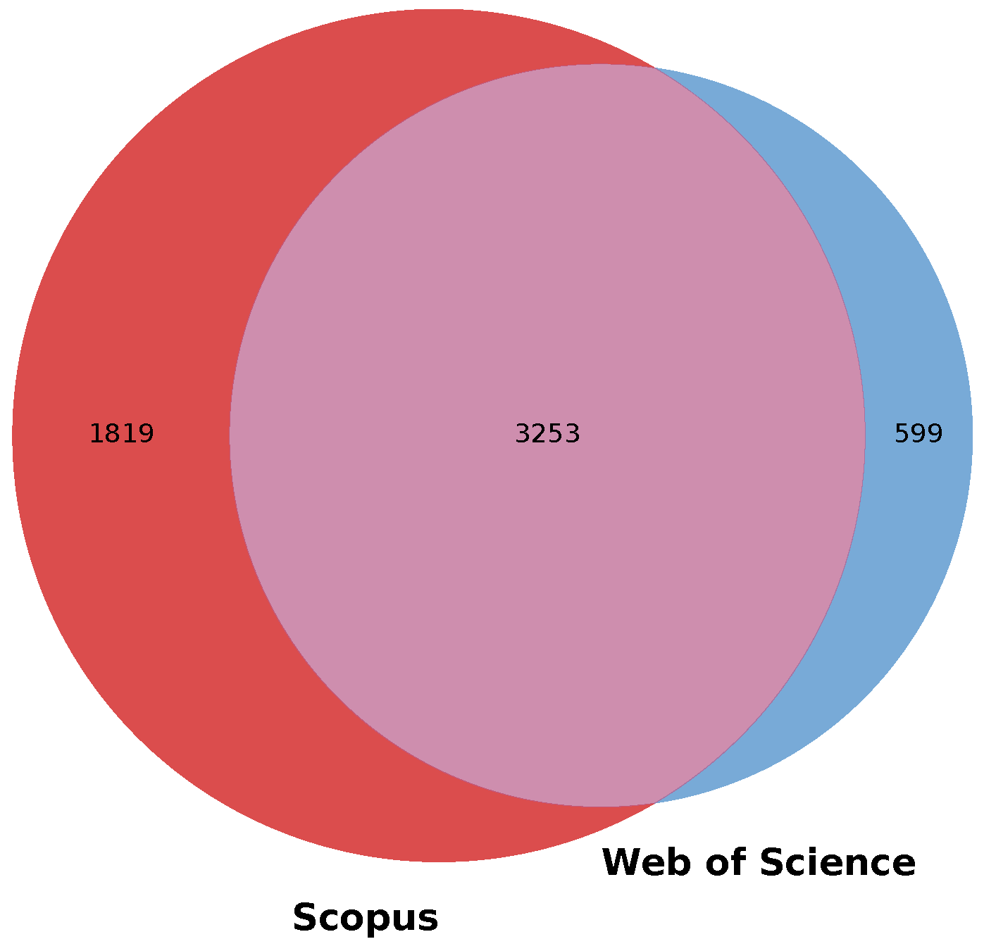
Figure 2.
PRISMA 2020 flow diagram for study selection [51].
Figure 2.
PRISMA 2020 flow diagram for study selection [51].
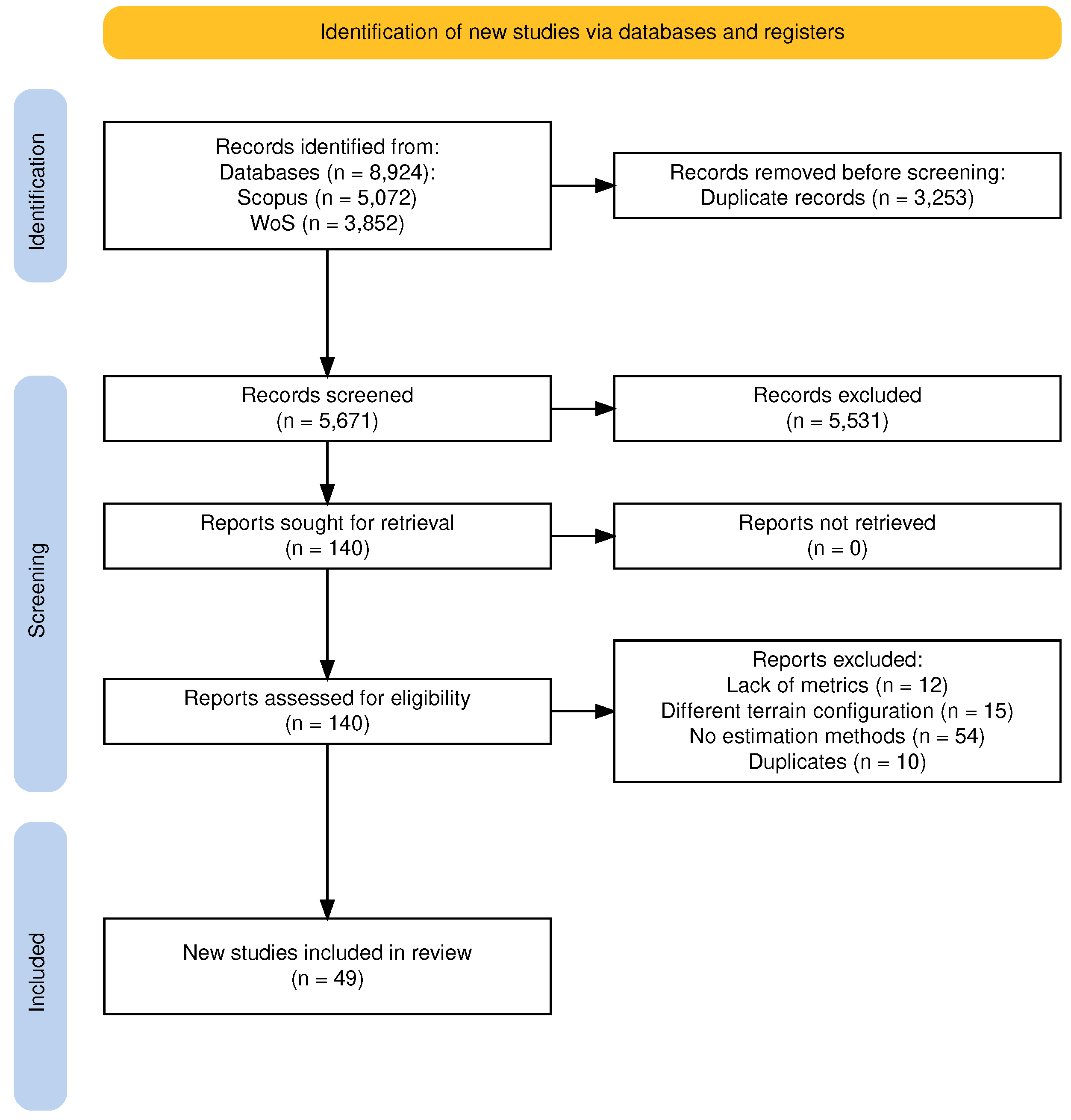
Figure 3.
Funnel Plot General.
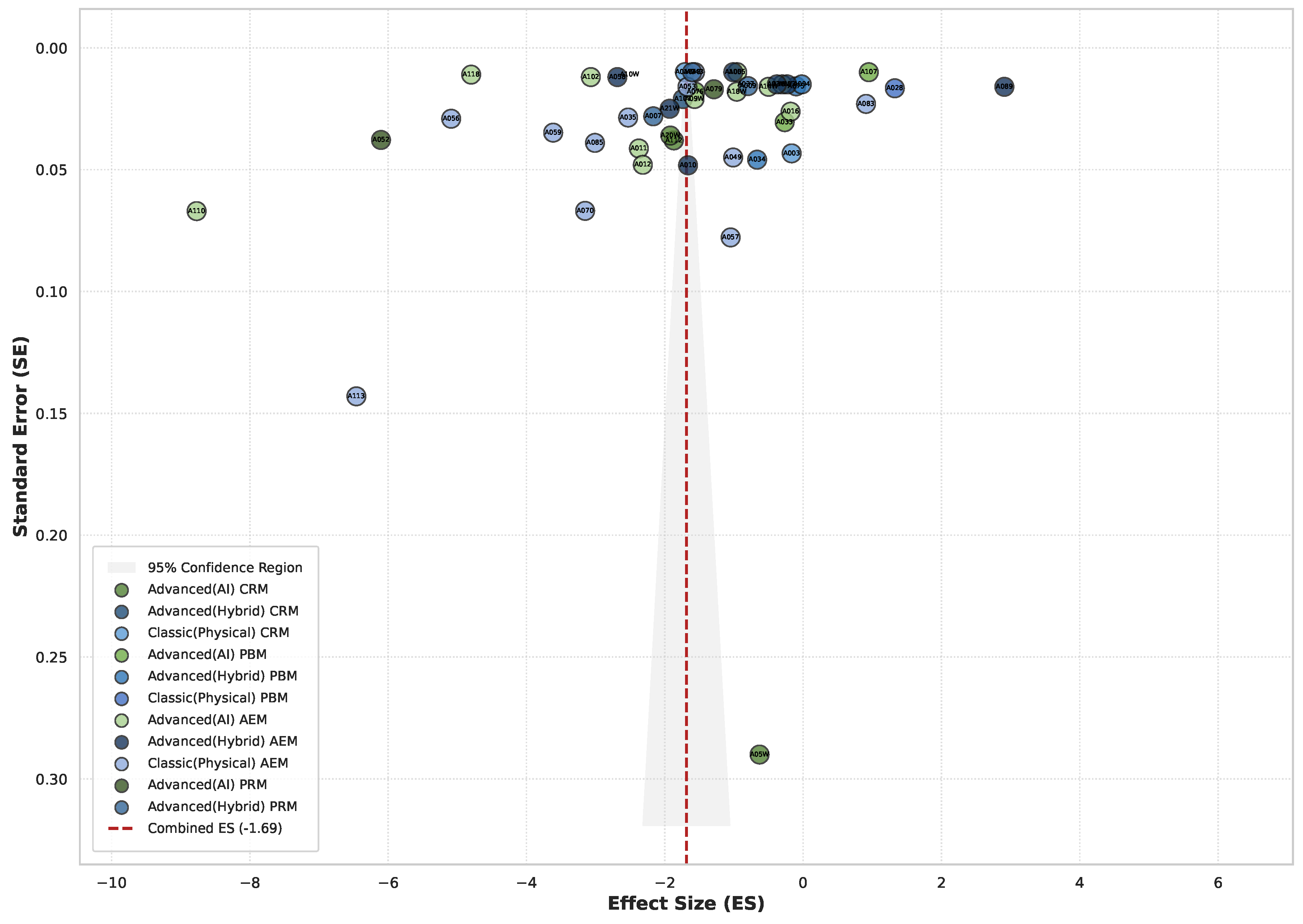
Figure 4.
QQ Plot General.
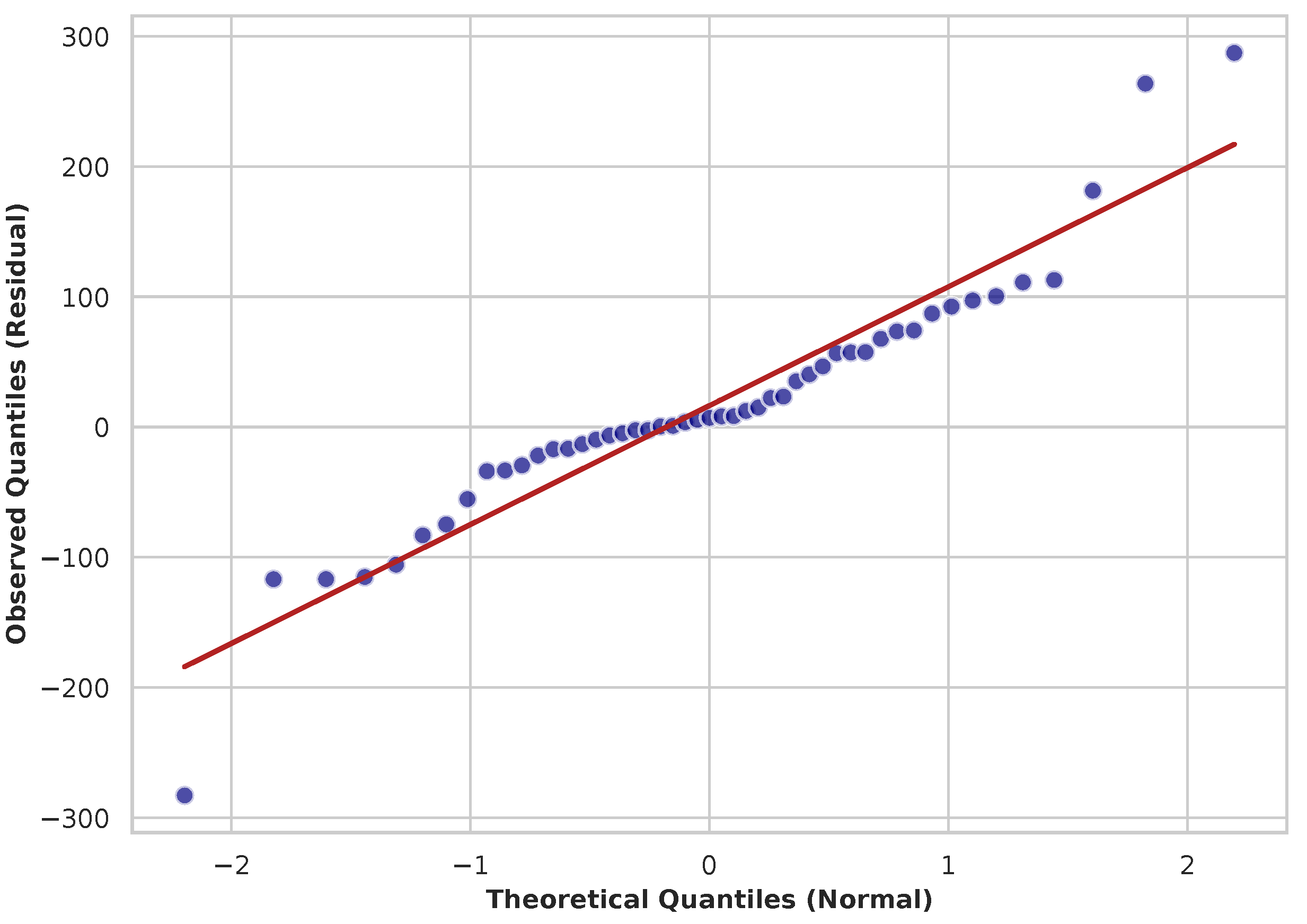
Figure 5.
Forest Plot General by Architecture.
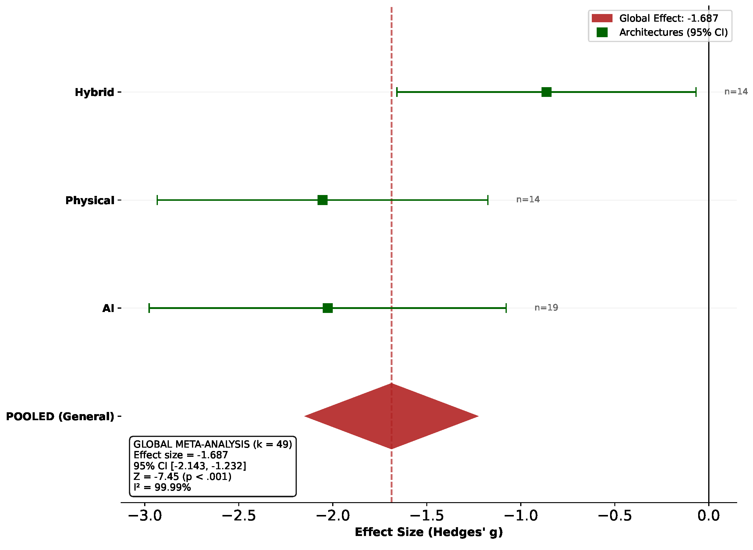
Figure 7.
Forest Plot of only subgroups and moderators.
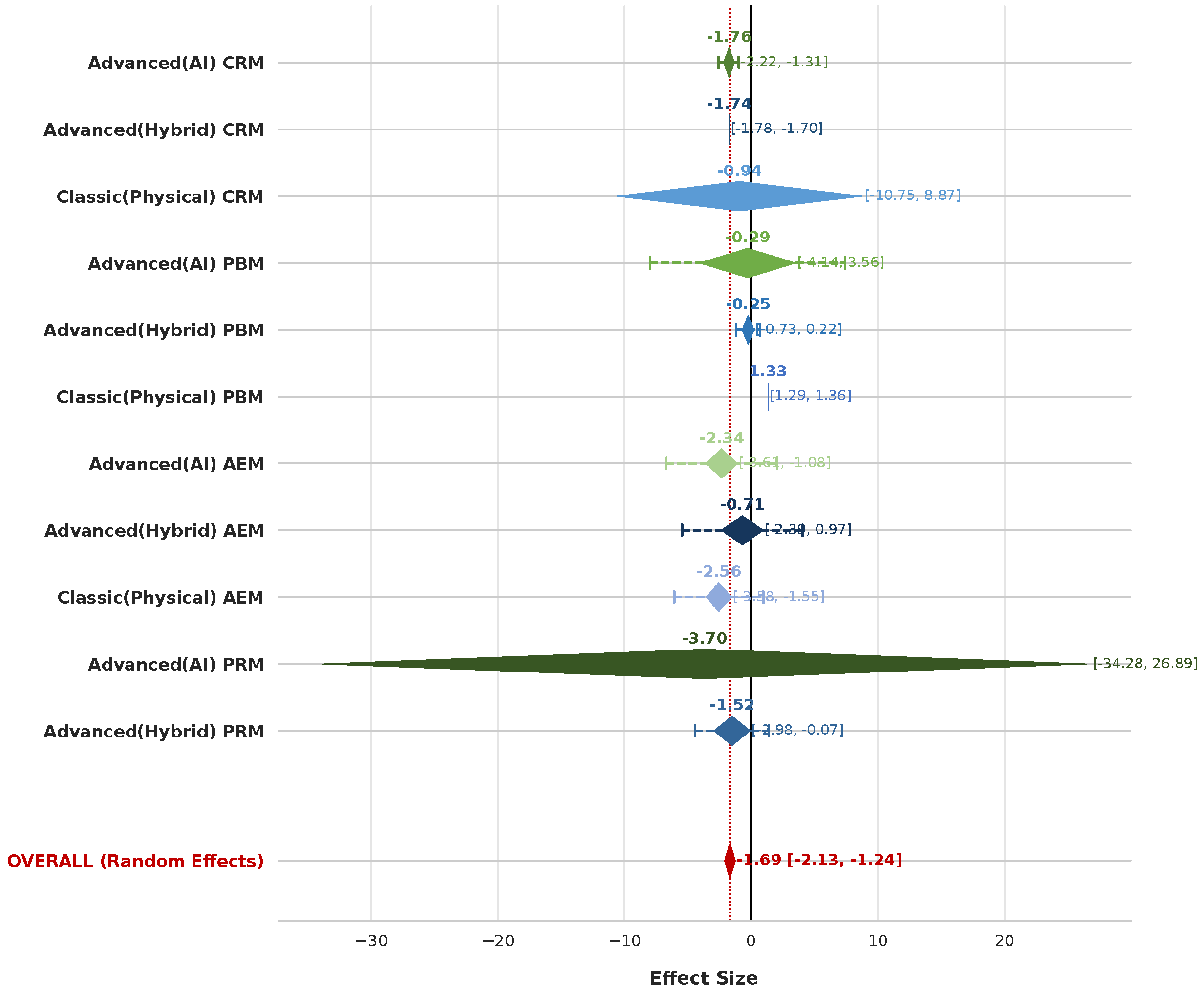
Figure 8.
Forest Plot General by Moderators.
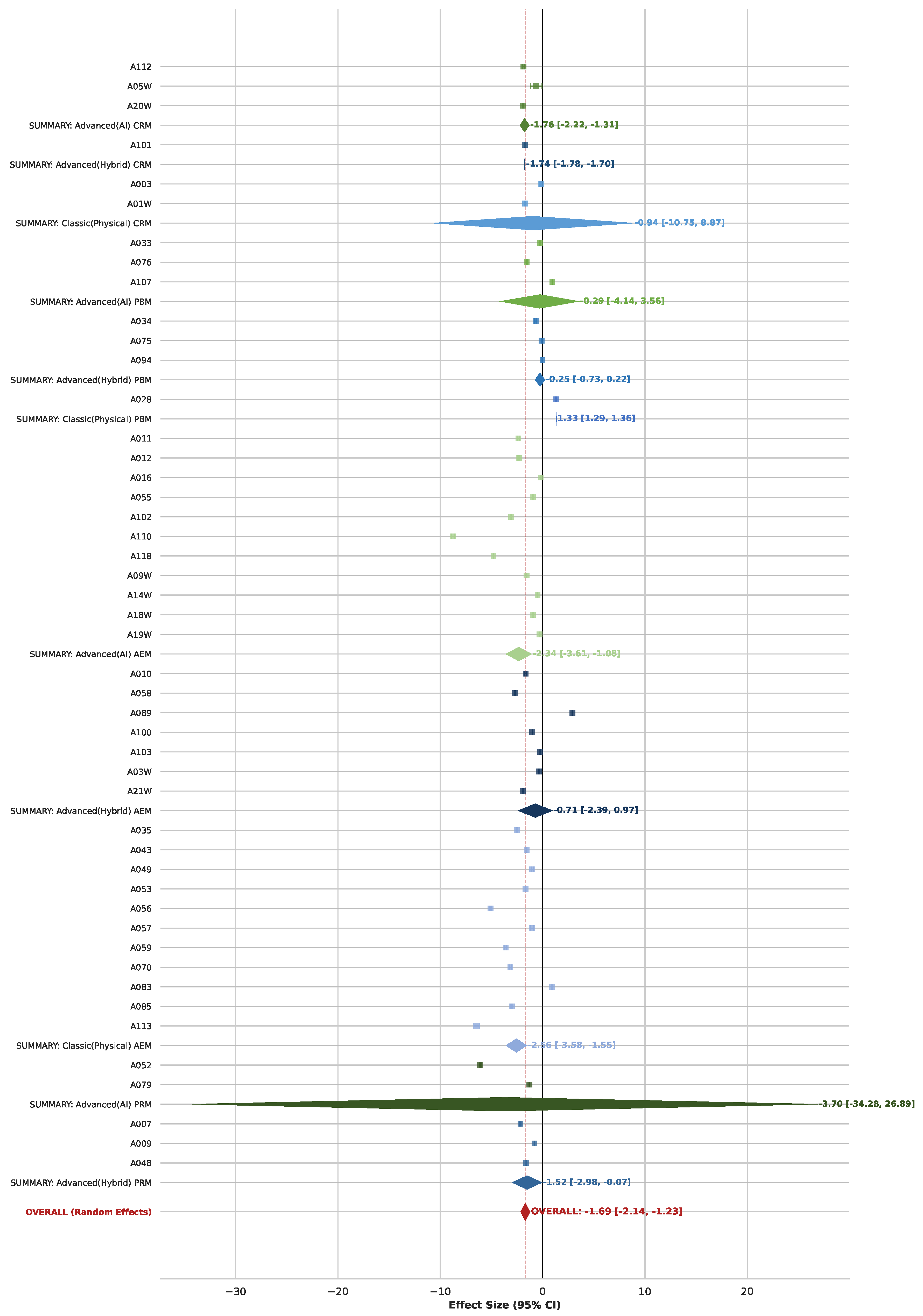
Figure 9.
Forest Plot General by Moderators without Massive N studies.
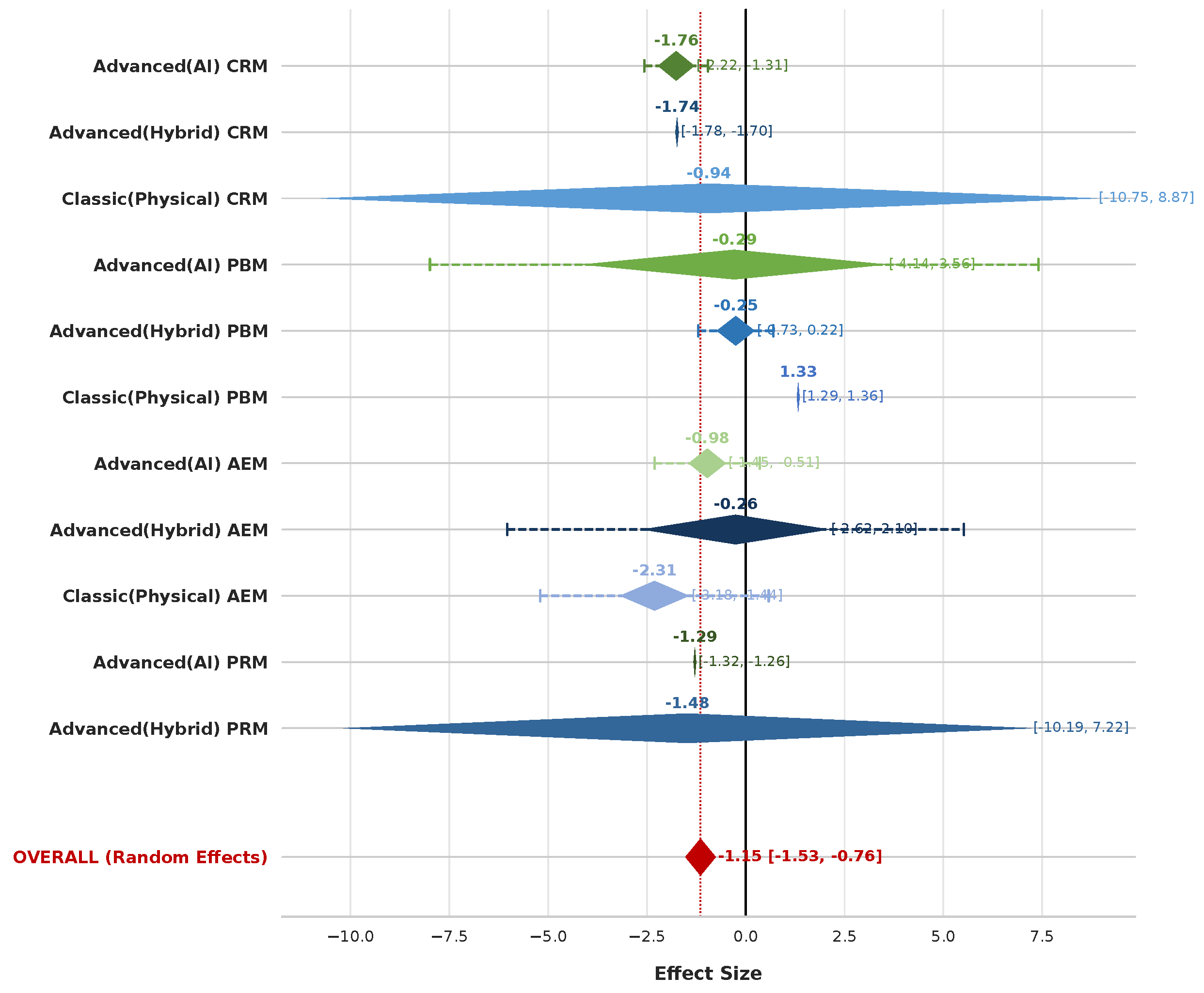
Table 1.
Search equations used by database.
| Database | Search Equation | Qty. Item | Last Query Date |
|---|---|---|---|
| Scopus | (TITLE-ABS-KEY ((("wind energy" OR "wind farm" OR "eolic power" OR "wind power forecasting" OR "wind speed prediction" OR "wind profile") AND ("complex terrain" OR "complex flow" OR "coastal zone" OR "offshore" OR "onshore" OR "trade wind*" OR "mountainous" OR "abrupt topography") AND ("model*" OR "predict*" OR "forecast*" OR "estimat*" OR "simulat*" OR "profil*" OR "map*" OR "assessment" OR "Naive" OR "physical model*" OR "numerical model*" OR "LES" OR "WRF" OR "mesoscale" OR "micrositing" OR "statistical model*" OR "multivariate" OR "ARMA" OR "ARIMA" OR "SARIMA" OR "SARIMAX" OR "GARCH" OR "SVM" OR "ELM" OR "Exponential Smoothing" OR "Gaussian Process" OR "AI" OR "ML" OR "DL" OR "machine learning" OR "deep learning" OR "neural network*" OR "RNN" OR "CNN" OR "LSTM" OR "GRU" OR "RBF" OR "Ensemble" OR "hybrid method*" OR "coupled model*" OR "ARMA-GARCH" OR "BA-BP" OR "EANN" OR "wavelet transform*"))) AND PUBYEAR > 2019 AND PUBYEAR < 2026 AND (EXCLUDE (DOCTYPE, "cp"))) | 5072 | 29/Jan/2026 |
| WoS | TS=(("wind energy" OR "wind farm" OR "eolic power" OR "wind power forecasting" OR "wind speed prediction" OR "wind profile") AND ("complex terrain" OR "complex flow" OR "coastal zone" OR "offshore" OR "onshore" OR "trade wind*" OR "mountainous" OR "abrupt topography") AND ("model*" OR "predict*" OR "forecast*" OR "estimat*" OR "simulat*" OR "profil*" OR "map*" OR "assessment" OR "Naive" OR "physical model*" OR "numerical model*" OR "LES" OR "WRF" OR "mesoscale" OR "micrositing" OR "statistical model*" OR "multivariate" OR "ARMA" OR "ARIMA" OR "SARIMA" OR "SARIMAX" OR "GARCH" OR "SVM" OR "ELM" OR "Exponential Smoothing" OR "Gaussian Process" OR "AI" OR "ML" OR "DL" OR "machine learning" OR "deep learning" OR "neural network*" OR "RNN" OR "CNN" OR "LSTM" OR "GRU" OR "RBF" OR "Ensemble" OR "hybrid method*" OR "coupled model*" OR "ARMA-GARCH" OR "BA-BP" OR "EANN" OR "wavelet transform*")) NOT DT=(Proceedings Paper) | 3852 | 29/Jan/2026 |
Table 2.
Results of the database filtering process with proportional overlap allocation.
| DB | Art. | Adj. Unique | F1 | % A1 | F2 | % A2 | F3 | % A3 |
|---|---|---|---|---|---|---|---|---|
| Scopus | 5072 | 3668 | 119 | 3.24% | 41 | 34.45% | 39 | 95.12% |
| WoS | 3852 | 2003 | 21 | 1.05% | 18 | 80.95% | 10 | 55.55% |
* Note: 3,253 overlapping duplicates distributed proportionally to DB initial search share. Total unique records = 5,671. % A1 = (F1 / Adj. Unique) * 100.
Table 3.
Meta-analysis results and model specifications.
| Metric / Parameter | Value / Detail |
|---|---|
| Model and Presentation | |
| Model Type | Random effects model |
| Confidence Level | 95% |
| Sort By / Order | Entry number / Ascending |
| Combined Effect Size | |
| Combined Effect Size | -1.6874 |
| SECES | 0.2265 |
| CI Lower Limit | -2.1427 |
| CI Upper Limit | -1.2320 |
| PI Lower Limit | -4.9053 |
| PI Upper Limit | 1.5306 |
| Statistical Significance | |
| Z-value | -7.4508 |
| One-tailed p-value | 0.0000 |
| Two-tailed p-value | 0.0000 |
| Number of included studies | 49.0000 |
| Heterogeneity | |
| Q | 403453.3180 |
| 0.0000 | |
| 0.9999 | |
| 2.5102 | |
| T | 1.5844 |
Table 4.
Translation table between study IDs and corresponding references.
| ID | Ref. | ID | Ref. | ID | Ref. | ID | Ref. |
|---|---|---|---|---|---|---|---|
| Scopus Set | |||||||
| A003 | [56] | A035 | [66] | A057 | [75] | A089 | [84] |
| A007 | [57] | A037 | [67] | A058 | [76] | A094 | [85] |
| A009 | [58] | A043 | [68] | A059 | [77] | A100 | [86] |
| A010 | [59] | A048 | [69] | A070 | [78] | A101 | [87] |
| A011 | [60] | A049 | [70] | A075 | [79] | A102 | [88] |
| A012 | [61] | A052 | [71] | A076 | [80] | A103 | [89] |
| A016 | [62] | A053 | [72] | A079 | [81] | A107 | [90] |
| A028 | [63] | A055 | [73] | A083 | [82] | A110 | [91] |
| A033 | [64] | A056 | [74] | A085 | [83] | A112 | [92] |
| A034 | [65] | A113 | [93] | ||||
| A118 | [94] | ||||||
| Web of Science Set | |||||||
| A01W | [95] | A05W | [97] | A10W | [99] | A18W | [101] |
| A14W | [100] | A19W | [102] | A03W | [96] | A09W | [98] |
| A20W | [103] | A21W | [104] | ||||
Table 5.
Comprehensive bias, regression, and sensitivity analysis.
| Model / Metric | Estimate | SE | CI LL | CI UL |
|---|---|---|---|---|
| Egger Regression (Linear) [] | ||||
| Intercept | 41.2276 | 60.2817 | -80.0436 | 162.4989 |
| Slope | -1.8503 | 0.7491 | -3.3572 | -0.3434 |
| Normal Quantile Regression | ||||
| Intercept | -69.6733 | 4.4335 | -78.5923 | -60.7544 |
| Slope | 91.3873 | 4.4913 | 82.3520 | 100.4227 |
| Rank Correlation (Begg & Mazumdar) | ||||
| Kendall’s Tau a | -0.2052 | |||
| Z-value | -2.0800 | |||
| p-value | 0.0398 | |||
| Rosenthal Fail-Safe Test | ||||
| Overall Z-score | -7.4508 | |||
| Fail-Safe N | 659.1 | |||
| Status () | Robust | |||
| Orwin Fail-Safe Test | ||||
| Criterion value ESC | -0.0500 | |||
| Mean fail-safe ESFS | 0.0000 | |||
| Fail-Safe N | 1605.0000 | |||
| Fisher Fail-Safe Test | ||||
| Fail-Safe N | 4206.0000 | |||
| p (Chi-square test) | ||||
Table 6.
Study distribution by main subgroup.
| No. | Subgroup | Quantity |
|---|---|---|
| 0 | Classic (Physical) | 14 |
| 1 | Classic (Statistical) | 0 |
| 2 | Advanced (Hybrid) | 14 |
| 3 | Advanced (AI) | 19 |
| 4 | Advanced (Ensemble) | 2 |
Table 7.
Verified meta-analysis results: summary by architecture.
| Architecture | Statistic | Value | 95% CI / Range |
|---|---|---|---|
| General () | |||
| Obs. g | -1.6874 | [-2.1427, -1.2320] | |
| Pred. Int. | — | [-4.9053, 1.5306] | |
| Heterog. | : 99.99% | : 2.5102 | Q: 403453.3180 | ||
| Bias | Egger p: 0.4974 | Begg p: 0.0398 | ||
| Failsafe-N | Rosenthal: 659.1 | Threshold: 255 | ||
| Robustness | Robust | ||
| Hybrid () | |||
| Obs. g | -0.8630 | [-1.6585, -0.0675] | |
| Pred. Int. | — | [-3.9434, 2.2174] | |
| Heterog. | : 99.99% | : 1.8975 | Q: 98730.5047 | ||
| Bias | Egger p: 0.2054 | Begg p: 0.6996 | ||
| Failsafe-N | Rosenthal: 6.0 | Threshold: 80 | ||
| Robustness | Low Robustness | ||
| Physical () | |||
| Obs. g | -2.0539 | [-2.9332, -1.1746] | |
| Pred. Int. | — | [-5.4573, 1.3495] | |
| Heterog. | : 99.98% | : 2.3162 | Q: 64804.0147 | ||
| Bias | Egger p: 0.4772 | Begg p: 0.2277 | ||
| Failsafe-N | Rosenthal: 78.8 | Threshold: 80 | ||
| Robustness | Borderline Robustness | ||
| AI () | |||
| Obs. g | -2.0268 | [-2.9764, -1.0772] | |
| Pred. Int. | — | [-6.2710, 2.2174] | |
| Heterog. | : 99.99% | : 3.8767 | Q: 213272.2783 | ||
| Bias | Egger p: 0.7313 | Begg p: 0.0861 | ||
| Failsafe-N | Rosenthal: 80.4 | Threshold: 105 | ||
| Robustness | Limited Robustness | ||
Table 8.
Comprehensive distribution of research models and subgroups.
| Metric Type | Quantity | Group Total |
|---|---|---|
| Classic (Physical) | ||
| AEM | 11 | 14 |
| CRM | 2 | |
| PBM | 1 | |
| Classic (Statistical) | ||
| — | 0 | 0 |
| Advanced (Hybrid) | ||
| AEM | 7 | 14 |
| CRM | 1 | |
| PBM | 3 | |
| PRM | 3 | |
| Advanced (AI) | ||
| AEM | 11 | 19 |
| CRM | 3 | |
| PBM | 3 | |
| PRM | 2 | |
| Advanced (Ensemble) | ||
| PRM | 2 | 2 |
| Grand Total | 49 | |
Table 9.
Verified meta-analysis results: summary by metric group.
| Group | Statistic | Value | 95% CI / Range |
|---|---|---|---|
| General () | |||
| Obs. g | -1.6874 | [-2.1427, -1.2320] | |
| Pred. Int. | — | [-4.9053, 1.5306] | |
| Heterog. | : 99.99% | : 2.5102 | Q: 403453.3180 | ||
| Bias | Egger p: 0.4974 | Begg p: 0.0398 | ||
| Failsafe-N | Rosenthal: 659.1 | Threshold: 255 | ||
| Robustness | Robust | ||
| AEM () | |||
| Obs. g | -2.0342 | [-2.7047, -1.3637] | |
| Pred. Int. | — | [-5.7057, 1.6373] | |
| Heterog. | : 99.99% | : 3.1055 | Q: 272186.9330 | ||
| Bias | Egger p: 0.4159 | Begg p: 0.0463 | ||
| Failsafe-N | Rosenthal: 262.5 | Threshold: 155 | ||
| Robustness | Robust | ||
| CRM () | |||
| Obs. g | -1.3776 | [-1.8522, -0.9030] | |
| Pred. Int. | — | [-2.6033, -0.1519] | |
| Heterog. | : 99.62% | : 0.1933 | Q: 1322.6213 | ||
| Bias | Egger p: 0.6783 | Begg p: 0.7194 | ||
| Failsafe-N | Rosenthal: 81.0 | Threshold: 40 | ||
| Robustness | Robust | ||
| PBM () | |||
| Obs. g | -0.0478 | [-0.9699, 0.8743] | |
| Pred. Int. | — | [-2.6551, 2.5596] | |
| Heterog. | : 99.97% | : 0.9934 | Q: 20600.8385 | ||
| Bias | Egger p: 0.1281 | Begg p: 0.1361 | ||
| Failsafe-N | Rosenthal: 0 | Threshold: 45 | ||
| Robustness | Low Robustness | ||
| PRM () | |||
| Obs. g | -2.1852 | [-3.1321, -1.2384] | |
| Pred. Int. | — | [-4.8628, 0.4923] | |
| Heterog. | : 99.98% | : 1.0477 | Q: 26619.8313 | ||
| Bias | Egger p: 0.6034 | Begg p: 0.5619 | ||
| Failsafe-N | Rosenthal: 51.1 | Threshold: 45 | ||
| Robustness | Robust | ||
Table 10.
Explanatory power of alternative moderator sets.
| Moderator Set | Residual | Analog (%) | AIC | Delta AIC |
|---|---|---|---|---|
| Metric + Sample Size | 1.6346 | 34.8835 | 196.5845 | 0.0000 |
| Metric + Control + Sample Size | 1.4943 | 40.4701 | 200.4425 | 3.8580 |
| Metric | 2.2810 | 9.1304 | 208.3739 | 11.7894 |
| Metric + Control | 2.0545 | 18.1539 | 212.6168 | 16.0323 |
| Control Family | 2.4675 | 1.7000 | 216.0190 | 19.4345 |
Table 13.
Comparative sensitivity analysis: full dataset vs. non-massive sample size subgroup.
| Metric / Statistic | Full Dataset | Non-Massive |
|---|---|---|
| Heterogeneity Statistics | ||
| Between Subgroups (Q) | 129,641.97 | 78,612.76 |
| Within Subgroups () | 273,811.35 | 82,641.47 |
| Total Heterogeneity () | 403,453.32 | 161,254.23 |
| Degrees of Freedom (df) | 48 | 38 |
| Combined Effect Size | ||
| Effect Size () | -1.6874 | -1.1458 |
| SE | 0.2265 | 0.1954 |
| 95% CI | [-2.1427, -1.2320] | [-1.5413, -0.7503] |
| 95% PI | [-4.9053, 1.5306] | [-3.6443, 1.3527] |
Table 14.
Representative configurations with large estimated effects across methodological paradigms.
Table 14.
Representative configurations with large estimated effects across methodological paradigms.
| Top | Study | Model | Result |
|---|---|---|---|
| Advanced AI | |||
| 1 | [94] | Random Forest | , |
| 2 | [71] | DBANN | , |
| 3 | [88] | ST-EDCNet | , |
| Advanced Hybrid | |||
| 1 | [69] | NWP+Random Forest | , |
| 2 | [76] | VMD-RUN-Seq2Seq | , |
| 3 | [86] | GAT-Informer-MTL | , |
| Classical Physical | |||
| 1 | [68] | Mod RSM | , |
| 2 | [95] | WRF-TC | , |
| 3 | [74] | HRRR/WRF | , |
Table 15.
Sensitivity of the global pooled effect to the between-study variance estimator.
| Estimator | Pooled g (95% CI) | Sig. | |
|---|---|---|---|
| DerSimonian–Laird (primary) | 2.5102 | [, ] | |
| Paule–Mandel | 4.0819 | [, ] | |
| REML | 4.0805 | [, ] |
* Note: Paule–Mandel and REML estimated on the 49 study-level effect sizes and standard errors reported in Table A1; the pooled point estimate and its statistical significance are stable across all three estimators.
Table 16.
Subgroup meta-analysis by prediction target.
| Target | k | Pooled g | 95% CI | |
|---|---|---|---|---|
| Wind Power Output (WPO) | 18 | [, ] | 99.99% | |
| Wind Speed Profile (WSP) | 26 | [, ] | 99.97% | |
| Atmospheric Conditions (ATM) | 5 | [, ] | 100% |
Table 17.
Pairwise contrasts between architecture-family pooled effects.
| Contrast | Difference | z | p-value |
|---|---|---|---|
| Physical vs. AI | 0.967 | ||
| Physical vs. Hybrid | 0.004 | ||
| AI vs. Hybrid | 0.053 |
Disclaimer/Publisher’s Note: The statements, opinions and data contained in all publications are solely those of the individual author(s) and contributor(s) and not of MDPI and/or the editor(s). MDPI and/or the editor(s) disclaim responsibility for any injury to people or property resulting from any ideas, methods, instructions or products referred to in the content. |
© 2026 by the authors. Licensee MDPI, Basel, Switzerland. This article is an open access article distributed under the terms and conditions of the Creative Commons Attribution (CC BY) license (http://creativecommons.org/licenses/by/4.0/).
Copyright: This open access article is published under a Creative Commons CC BY 4.0 license, which permit the free download, distribution, and reuse, provided that the author and preprint are cited in any reuse.