
Submitted:
10 September 2026
Posted:
13 September 2026
You are already at the latest version
Abstract
While polynomial interpolation discretizes fractional operators up to order \(k-\alpha\) (\(k=4,5,6,7\)), we construct a \(4-\alpha\) order approximation for the Caputo derivative directly in the frequency domain using the asymptotic expansion of the polylogarithm function. We determine the scheme's weights by applying the method of undetermined coefficients to a polynomial correction of the generating function \(\operatorname{Li}_{1+\alpha}(e^{-z})\), which cancels low-order truncation errors. To address the continuous solution's initial weak singularity near \(t=0\)—a persistent issue that degrades theoretical \(\mathcal{O}(\tau^{4-\alpha})\) accuracy to first order—we introduce a starting correction that modifies the right-hand side of the discrete equations. Although this modification applies solely to the first three time steps, Laplace transform analysis establishes the uniform recovery of the optimal \(\mathcal{O}(\tau^{4-\alpha})\) convergence rate for any fixed \(t>0\). Numerical tests on both homogeneous and inhomogeneous equations confirm this result.
Keywords:
time-fractional subdiffusion equations
; starting correction
; discrete Laplace transform
MSC: 65M06; 65M12; 35R11
1. Introduction
This paper is concerned with the development and analysis of high-order time-stepping discrete methods for the following initial-boundary value problem of the subdiffusion equation [1,2]:
where () is a convex polygonal or polyhedral domain with boundary , and is a fixed number. Here, is a given source function, and is a given initial data. The operator is the negative Laplacian defined on the domain . is the left-sided Caputo fractional derivative of order , defined by [9]
where denotes the Euler Gamma function. The subdiffusion equation is a valuable tool for describing slow transport processes in complex systems, including subsurface environments, turbulent plasmas, and heterogeneous porous media [1]. To capture such anomalous behavior accurately, high-order time discretization schemes are often essential, especially when the data are nonsmooth [2].
Finite difference methods for the Caputo fractional derivative mainly fall into two classes: L1-type and Grünwald-Letnikov-type schemes. The former handles variable coefficients and nonsmooth data more flexibly. Within the L1 framework, the standard scheme achieves order for smooth solutions, whereas the L1-2 formula raises this to via quadratic interpolation [4]. However, these polynomial-based schemes demand high regularity. As noted in [3], solutions typically exhibit weak singularities near . Without strict compatibility conditions, this singular behavior severely degrades the convergence rate of high-order methods down to first order.
The Laplace (or Fourier) transform of fractional calculus yields (or ) [9], motivating the approximation of fractional derivatives directly from the frequency domain. Generating functions facilitate this approach by mapping discrete operators into the Laplace domain. Recent developments heavily utilize the Riemann zeta and polylogarithm functions. Dimitrov et al. [7] constructed a -order approximation using the polylogarithm, and subsequently [8] derived an equivalent-order scheme via asymptotic expansions involving . These approaches endow the discrete weights with explicit integral representations. Such exactness significantly simplifies the subsequent error analysis.
We extend the zeta/polylogarithm framework of Dimitrov et al. [7,8] by constructing a family of generating functions of order (). This leads to our new time-stepping methods, the Zeta schemes. We then incorporate the starting correction technique of [12] directly into the discrete convolution. This specific modification alters both the generating function and the Laplace-domain integration contour, compensating for the initial singular behavior. To further suppress truncation errors stemming from the dominant singularity, we introduce an additional correction factor. A linear system involving the Riemann zeta function determines the necessary correction coefficients to cancel the leading errors. By employing contour integral techniques, we prove that the corrected schemes uniformly recover the optimal rate for any fixed . Remarkably, this optimal convergence holds for both homogeneous and inhomogeneous problems, even when dealing with incompatible initial data and nonsmooth sources.
The remainder of this paper is organized as follows. Section 2 and Section 3 detail the time discretization. Here, we introduce the starting correction terms and compute the coefficients needed for the high-order generating function. Section 4 and Section 5 contain the core theoretical analysis: deriving uniform error estimates for the homogeneous and inhomogeneous cases, respectively, alongside the high-order correction factor. Section 6 presents numerical experiments that validate our theoretical bounds. Section 7 gives a brief conclusion.
2. High-Order CQ schemes
2.1. Pre Knowledge
Let and be the value of the function at the point . The L1 approximation of the Caputo derivative is constructed by dividing the interval into subintervals of equal length and approximating the first derivative on each subinterval using a second-order central difference approximation.
For any sequence , let denote the generating function of the sequence defined by
The L1 approximation formula is given by
where , , and (). The popular L1 scheme [3] is associated with the generating symbol
where
is the polylogarithmic function, which is well defined for and can be analytically continued to the split complex plane .
The CQ generated by the k-th order BDF [10,11] is given by formal power series expansions. To establish our high-order CQ approximations, we rely on the following asymptotic summation behavior and singularity expansions.
Lemma 1.
[13] If , then
In particular, if for , then
Lemma 2.
[24] For , the function satisfies the singular expansion
where ζ is the Riemann zeta function.
Proof.
To establish the absolute convergence of the series in a neighborhood of , we employ the functional equation for the Riemann zeta function:
As , the argument , which implies . Furthermore, by Stirling’s formula (or the asymptotic ratio of Gamma functions), we have as . Consequently, the general term of the series satisfies
for some constant . By the ratio test, this power series has a radius of convergence . Since we are concerned with the asymptotic behavior as , the series converges absolutely in this domain. □
In particular, taking in Lemma 2, we obtain the specific singular expansion
2.2. High-Order Time Discretization Schemes
Inspired by the corrected scheme in [13] and drawing on the idea of polynomial interpolation, we construct new corrected schemes for both smooth and nonsmooth cases based on Lemma 1. The key idea is to regard the convolution weights of the discrete scheme as the coefficients of a power series , which is understood in the sense of formal power series for the purpose of asymptotic expansion.
Theorem 1.
Let and let be a given integer. Assume that the function and its derivatives up to order k vanish at . Construct the generating function
where the coefficients are uniquely determined by the equations
Then the convolution scheme whose weight coefficients are derived by ,
has order accuracy.
Proof.
We carry out the analysis in the frequency domain. Define the error symbol
where z lies on a suitable contour in the left half-plane. It suffices to show that as , uniformly on the contour. The desired time-domain estimate then follows by applying the inverse Laplace transform together with standard Paley–Wiener type arguments.
Since , we have
Substituting the explicit form of F, we obtain
Using the expansion
and
we have
Truncating high order terms for accuracy yields
Thus,
To achieve , it is necessary and sufficient to let the first several terms of the above expansion vanish. Factoring out the common multiplier from the summation, the condition reduces to:
Finally, applying the inverse Laplace transform gives the time-domain error estimate
This completes the proof. □
Since , we extend the solution by zero for negative times to derive the numerical scheme. We have
i.e.,
We now discuss special cases corresponding to indices . Solving the equations
by taking , we get and , yielding the weight coefficients
By means of the generating function, we obtain the same result as in [13].
If we take , the system of equations is rewritten as
Solving the equations yields , , and , which imply
If we take and solve the equations, namely,
we get
which imply the weight coefficients
To remove the stringent requirement that for all , we introduce a corrected scheme that is applicable to smooth solutions without such boundary restrictions. Designed along the local singularity matching principle of Jin et al. [12], this strategy applies specific algebraic weights directly to the right-hand side. Denoting the spatial operator by and setting , the corrected scheme for the homogeneous equation reads
where the correction coefficients are
and for .
For the inhomogeneous equation the correction involves the source function and its derivatives at :
For the right-hand side reduces to . Matching the Taylor expansion of at with the homogeneous correction factors gives the relation
If we take , we have
If we take , we get
If we take , we get
Example 1.
To confirm the theoretical convergence order of the above high-order discrete operators, we test a compatible configuration without temporal singularity. The initial condition is set to zero, , and the source term is taken as . Under this choice, the first temporal derivatives of f vanish identically at . Consequently, the exact solution possesses sufficient regularity at the origin and the scheme attains its formal convergence order without any starting correction.
All computations are performed with the Multiprecision Computing Toolbox (MP) at 100 decimal digits of precision, in order to circumvent the truncation limit imposed by standard IEEE 754 double-precision arithmetic. The reference solution is computed with the fully corrected scheme on a uniform mesh with for all k.
For clarity of presentation, Table 1 reports the results on the test grids together with the corresponding convergence rates. On the finest grids, the errors approach the double-precision machine floor (); points falling below are excluded from the rate computation to avoid contamination by round-off. Notably, for the scheme, the extreme decay rate limits the valid data to only a few points before hitting the noise floor, yet the estimated rates remain theoretically consistent.
The convergence rates in Table 1 confirm that, once the singular barrier at the initial time is removed, all higher-order Zeta discrete operators attain the formal convergence order under sufficiently fine grids and high-precision arithmetic. This confirms that the discrete operators themselves attain the formal convergence order, independently of any starting correction. In future work, we will investigate generalized multi-point starting correction strategies for these higher-order () discrete operators under incompatible source terms and nonsmooth initial data.
Remark 1.
For (), is computed directly from the Dirichlet series, which incurs a truncation error bounded by for N terms. For , the functional equation (59) reflects the arguments to , enabling evaluation via the absolutely convergent reflected series. For , the argument maps to , which remains in the critical strip ; here, evaluation typically relies on the Euler–Maclaurin summation or the alternating Dirichlet eta function. All four constants are evaluated exactly once at cost independent of the time-step count, with robust implementations readily provided by standard numerical libraries.
3. High-Order CQ Schemes
The definition of the Caputo derivative can be rewritten to establish the relationship:
By introducing the homogenized variable , we obtain the equivalent system with the Riemann-Liouville derivative:
with the left-sided Riemann-Liouville fractional derivative of order defined by
To analyze this system, we utilize the continuous Laplace transform and its associated properties. Since , the Caputo and Riemann-Liouville derivatives coincide. Assuming that the exact solution is analytically extendable to the sector , the Laplace transform of the fractional derivative is well-defined as
where the frequency variable z belongs to the sector with . We define the spatial operator A as a self-adjoint positive definite second-order elliptic operator with dense domain in . As a strongly elliptic operator, A is sectorial: there exists an angle such that the resolvent estimate
holds uniformly for all z in the sector . Consequently, A generates a bounded analytic semigroup, which implies that the solution can be analytically extended to a sector containing the positive real axis. This justifies the use of the Laplace transform and contour integration in the complex plane.
We now fix an angle sufficiently close to . For and any , we have ; thus . Replacing z by in the resolvent estimate, we obtain
valid for all , where C depends only on and . From the operator identity , which follows directly from the commutativity of A with its resolvent, we obtain a key relation for subsequent contour integral estimates.
Applying the Laplace transform to (Section 3) yields . Let be the sectorial contour defined by
oriented with an increasing imaginary part, where . Then, by taking the inverse Laplace transform along this contour, the function can be represented as
with the kernel function defined by
To approximate the fractional derivative, we employ a high-order convolution quadrature approximation characterized by the generating function. For the sake of simplicity in the error analysis, we now focus on the homogeneous case (). Following the continuous formulation introduced earlier, we directly seek the fully discrete solution at time level with the initial condition . The fully discrete evolution scheme satisfies
where denotes the discrete initial data. Multiplying both sides of the equation by and summing from to ∞ yields
where and is the generating function. Using the fact and the discrete convolution property of generating functions, the first term on the left-hand side can be directly expressed as . This leads to the frequency-domain algebraic equation:
Extracting the common factor, the generating function of the fully discrete solution can be represented in the form of a resolvent operator:
It is easy to verify that the function is analytic at . Hence, Cauchy’s integral theorem implies that for sufficiently small , there holds
Upon changing the variable , we obtain
where the contour corresponds to the counterclockwise orientation in the -plane. By continuously deforming the contour to and using the periodicity of the exponential function (which ensures that the integrals along the horizontal segments perfectly cancel each other), we obtain
This integral representation forms the foundation for the subsequent error analysis and kernel function estimation.
Lemma 3.([10,11]) The term denotes the Riemann zeta function. For , it is defined by the absolutely convergent Dirichlet series
It extends analytically to a meromorphic function on whose only singularity is a simple pole at . For , the analytic continuation satisfies the functional equation
Consequently, for any fractional parameter and integer , the evaluations are finite, well-defined real constants. These constants uniquely determine the high-order correction coefficients for the generating function , as explicitly derived earlier.
Lemma 4.
Let and define the discrete fractional derivative operator associated with the fully discrete order Zeta scheme as . Assume that there exist a positive constant and an angle independent of τ, such that for any with , the discrete operator satisfies and . Furthermore, as verified numerically in Figure 1, we assume has no zeros. Under these hypotheses, for all , the spectral equivalence holds:
Proof.
By the hypothesis of the lemma, we directly obtain the lower bound for all . To establish the upper bound, we first evaluate the limit as . Multiplying the numerator and denominator by , we have:
Therefore, there exists a constant such that holds for and .
On the other hand, when , we have with being sufficiently close to . In this case, the modulus satisfies:
Combining this bounded domain with the empirical boundedness of the generating function verified in Figure 1, we obtain the upper bound:
This completes the proof. □
Lemma 5.
For the discrete operator defined in Lemma 4, and for all z on the low-frequency contour portion , there exists a positive constant C independent of τ such that the truncation error satisfies
Proof.
From the frequency-domain discrete scheme, the truncation error can be expanded via the generating function. By the high-order construction of matching the fractional derivative symbol, the low-order error terms are precisely cancelled. Thus, for , we have:
Since is bounded by , the remainder of the power series is uniformly bounded, leading directly to the bound . This completes the proof. □
Theorem 2.
Let and let , extended by zero to . Here is the Sobolev space of functions whose weak derivatives up to order 4 are integrable on ; the zero extension implies for . Assume the Laplace transform is initially analytic for and admits an analytic continuation to a domain encompassing the integration contour . Assume further that the rapid decay of ensures . The truncation error of the order discrete operator satisfies
where the constant is independent of τ and n. The discrete weights are the corresponding coefficients of the generating function , whose explicit formulations incorporated with the high-order corrections have been provided. Here, the order discrete fractional approximation operator at is defined as:
Proof.
By the causality condition, and its derivatives up to order 3 vanish at , ensuring . The exact Caputo derivative and the discrete approximation operator evaluated at are expressed as:
Subtracting the exact derivative from the discrete operator yields the absolute truncation error:
where . We partition the contour into and .
On , Lemma 5 directly yields
On , the condition gives . Furthermore, for all , the mapped variable forms a compact set strictly bounded away from the singularity at . Recall from its explicit formulation (as defined in Lemma 3.3) that the generating function consists of polynomials and the polylogarithm , which admits an analytic continuation to the split complex plane . Since for all , is analytic in this compact region. Therefore, the extreme value theorem guarantees its uniform boundedness, i.e., . By the triangle inequality, . We bound the two terms separately. Since , we have
Raising to the power gives
Remark 2.
The decay assumption on stated earlier ensures the integral remains uniformly bounded as . This guarantees the theoretical asymptotic rate. For practical computations with any fixed , the truncation naturally restricts to a compact set. The continuous integrand thus trivially yields a finite integral.
Remark 3.
The preceding error estimate relies on the assumption that the initial data and its derivatives up to order vanish at . If any for , the exact solution typically exhibits weak singularities at the initial time, which leads to a severe order reduction in the standard convolution quadrature. Instead of modifying the last few terms of the convolution sum, we are inspired by Jin et al. [12], who introduced starting correction terms in the time domain to construct high-order schemes. Motivated by this, we propose a novel approach: directly matching and constructing the starting correction terms in the frequency domain to neutralize the initial singularities. The specific construction and detailed rigorous analysis of this modified scheme will be presented in the subsequent section.
4. Corrected Schemes for Homogeneous and Inhomogeneous Problem
In this section, we derive optimal error estimates for the fully discrete scheme. The analysis is based on the representations of the semidiscrete solution and the fully discrete solution . Subtracting the two gives:
where the terms I and are given by
and
Here the integral kernel functions and are defined by
where
and
Since is uniformly bounded and decays exponentially on , it suffices to bound . We first derive estimates for the auxiliary function and the high-order discrete operator.
4.1. Error Analysis of the Uncorrected Scheme
Lemma 6.
Let . Then for all , there hold for some
Proof.
We note that for . By means of Taylor expansion, the first assertion follows directly:
Next we consider the second claim. The upper bound of is trivial, so it suffices to verify the lower bound. Split the contour into three disjoint parts: . For , with . By , we obtain
due to the positivity and monotonicity of as a function of over the interval . The case of follows analogously. Last, we consider , the circular arc. In this case, by means of Taylor expansion, we have . From this and the fact that , it follows directly that . This completes the proof of the lemma. □
To estimate the spatial resolvent term , we define the high-order discrete kernel .
□
Lemma 7.
Let and . Then for any , there holds:
Proof.
Using the operator identity , we can rewrite the operators as:
By subtracting them and inserting cross terms, we obtain
Based on the resolvent estimate of the sectorial operator and the bound provided that , we deduce:
we finally arrive at .
□
Lemma 8.
Let and . Then for any , there holds
Proof.
By subtracting the operators and inserting a cross term, we decompose the norm as:
From Lemma 3.1, and . Together with the sectorial resolvent estimate , the first term is bounded by . For the second term, we apply the high-order bound from Lemma 4.2. Note uniformly on , with . Thereforce:
This completes the proof.
□
Theorem 3.
Let and be the semidiscrete and fully discrete homogeneous solutions, respectively. Then the total temporal discretization error satisfies .
Proof.
The total error is decomposed into . By the preceding lemmas, we estimate directly:
Using the change of variables (), we have:
Since the integral converges to a finite constant independent of , we obtain .
Similarly, the error for term I is bounded by:
Applying the identical substitution , we compute:
By the triangle inequality , the proof is complete. □
Remark 4.
The proof shows that although the CQ operator in the high-order scheme attains accuracy, the overall truncation error is dominated by the error between z and in the first term. This forms the algebraic bottleneck for further accuracy improvement.
4.2. Corrected Schemes for Nonsmooth Problems
In the generating function framework, the discrete time-stepping operator is encoded in the function
which appears in the contour integral representation of the numerical solution. Let be the continuous solution kernel and the kernel induced by the standard L1 discretisation. As established in Lemma 4.3, the discrepancy between these two kernels satisfies
The root cause of this saturation is the first-order accuracy of as an approximation to z, namely . To break this barrier we replace by a corrected prefactor that approximates z to higher order, thereby realigning the accuracy of the two kernel layers in the contour integral representation.
The construction starts from the elementary identity
Expanding the logarithm with the Mercator series and substituting yields the formal power series representation
Truncating the infinite series at the K-th term defines the order-K correction prefactor
By construction the residual satisfies
because . The integer K controls the formal accuracy: larger K eliminates more low-order error terms in the kernel expansion.
Setting in (99) gives the explicit expression
For the subsequent analysis it is convenient to introduce the scaled variable
so that and consequently
The function is precisely the K-th order Taylor polynomial of centred at . For , factoring out the common factor yields
where is the cubic polynomial
On the rays of the integration contour defined in Lemma 10 below, we have , hence . For the error analysis it is essential that does not vanish on the contour. By the factorisation (104) this is guaranteed if has no root inside the closed unit disk . The following classical result [15,16] provides a convenient sufficient condition.
Lemma 9.
where is the reciprocal polynomial of , and , denote respectively the constant term and the leading coefficient of . If the strict inequalities
hold for every step, then all roots of lie strictly outside the unit disk .
We apply Lemma 9 to (clearing the denominator does not affect the root locations). The coefficients are
For , . The reciprocal polynomial is , hence
For , . With ,
For , . All three inequalities are satisfied. Lemma 9 therefore guarantees that every root of , and consequently of , lies strictly outside . Thus for all z on the rays where , we have . Since on these rays, (104) implies , which is equivalent to by (103).
Lemma 10.
Let Γ be the Hankel-type contour consisting of the two rays
and a connecting circular arc of radius . Define . For and every , there exist constants , independent of τ, such that
and the approximation error satisfies
Proof.
Set . From (103), . Truncating the Mercator series at gives
Since , we have , and therefore
Hence , which directly implies , proving (113).
We now turn to (112). On the rays , and . As shown above, and , so . Define for , and . The function F is analytic on the compact set and never vanishes there. By the extreme value theorem, there exist with
Multiplying by yields (112) on .
On the circular arc , . Because , we may select sufficiently small so that for all . The triangle inequality then gives , which translates to on . Combining the estimates on the three pieces of completes the proof. □
The same construction principle applies to any fixed order . The polynomial , defined implicitly by , can be verified to satisfy the Schur–Cohn criterion for each fixed K by a finite number of elementary operations, guaranteeing that on the contour. The resulting prefactor then achieves , providing a systematic route to arbitrarily high-order starting correction schemes.
Lemma 11.
Let . Assuming the fractional order is and the time step satisfies for a fixed final time T, for any , there exists a constant such that
Proof.
By subtracting the operators and inserting a cross term, the norm decomposes as:
From the mapping bounds : and . Given the spatial resolvent norm , the first term yields:
From the spatial approximation bound, . For the second term, we have
Summing these bounds completes the proof.
□
Theorem 4.
Let be the fully discrete homogeneous solution of the corrected scheme.For nonsmooth initial data , the -norm temporal discretization error satisfies:
Proof.
The total error in the -norm is decomposed into the outer and inner contour integral components .
For the inner contour integral , substituting the kernel difference bound from Lemma 4.2 yields
Utilizing the properties of the Gamma function, the above integral can be evaluated as
This derives .
For the outer contour integral I, on we have . Extracting the Kth-order temporal scaling term gives . Combining with the resolvent estimate and matching orders yields
The lower integration limit to 0 gives a strict upper bound:
By the triangle inequality , and recognizing that for the given fractional parameter the term dominates the overall truncation error, the theorem is proved. □
□
4.3. Corrected Scheme for Smooth Cases
Having discussed the space estimates for non-smooth initial data, we now address the problem under smooth initial conditions. Here, we define .
Lemma 12.
Let the continuous and discrete smooth kernel functions be defined as and , respectively. For any , there exists a constant such that:
Proof.
Utilizing operator difference, the norm is bounded by:
where and . For the first term, from previous bounds, it is easy to obtain
For the second term, applying the resolvent identity along with the operator estimates yields:
Combining both terms strictly derives . □
Theorem 5.
Let be the numerical solution under the corrected scheme. For smooth initial data with , the total error measured in the -norm satisfies:
Proof.
The error is decomposed into the outer and inner contour integrals :
Analogous to the proof strategy for in Theorem 4.5, the inner integral can be bounded as
Similarly, for the outer integral , extracting the 4th-order scaling term and using smooth-state estimates gives
Combining bounds for and via the triangle inequality, the scheme attains the optimal temporal convergence order . □
Remark 5.
Theorems 4 and 5 reveal the core difference in error behavior of the corrected scheme between nonsmooth initial data and smooth initial data . With higher spatial regularity, the singularity of the temporal discretization error as weakens from to . The singularity persists even for smooth initial data, reflecting the limited smoothing effect of the fractional derivative operator.
The high-order discrete symbol is constructed to approximate the continuous fractional operator with accuracy. For the homogeneous problem, the equivalent constant source term has a low-frequency truncation deficit in the discrete Laplace domain. To correct this, we perform high-order asymptotic expansion of the discrete generating function as .

Table 2.
Starting correction coefficients for the K-th order corrected schemes.
| K | ||||||
|---|---|---|---|---|---|---|
Table 3.
Starting correction coefficients for high-order Zeta schemes.
| K | ℓ | ||||||
|---|---|---|---|---|---|---|---|
5. Error Analysis for the Inhomogeneous Problem
We now extend the corrected scheme to the inhomogeneous equation,where and . The homogeneous problem treated in the previous sections corresponds to the special case , i.e., a constant source.
The correction coefficients were determined in Section 4.1 by requiring that the homogeneous scheme be exact for the leading singular modes of the continuous solution. For the inhomogeneous equation the source is no longer constant; its variation in time introduces additional low-order errors that must also be compensated. The key observation is that, by linearity, the correction for a variable source can be obtained by Taylor-expanding about and correcting each monomial term individually.
Assume that g is sufficiently smooth and write
where the remainder does not affect the leading-order error and requires no correction. Evaluating (132) at the discrete time levels gives
The constant term is precisely of the same form as the homogeneous source ; its correction is therefore identical to the homogeneous case. The terms involving are new and require separate treatment.
Consider the contribution of the ℓ-th derivative term to the right-hand side. At time this term evaluates to . In the continuous equation, the response of the system to a source proportional to is times weaker than its response to a constant source of the same pointwise magnitude. Consequently, the correction needed for this term inherits the same relative factor as the constant-source correction, weighted by the Taylor coefficient . Formally, matching the discrete correction term with the Taylor contribution yields the relation
For , and consequently for all ℓ; no correction is applied beyond the third time step.
Theorem 6.
Let be the numerical solution of the corrected fully discrete scheme and the exact continuous solution. Suppose (which implies ) and .
There exists a constant , independent of τ and h, subject to the initial condition (such that ), such that for all
Proof.
The Taylor expansion of the total source term at gives
where .
Using the Laplace transform identity , we obtain
where .
The exact continuous solution is given by the inverse Laplace transform
Applying the discrete Laplace transform (where ) to the fully discrete scheme yields . To incorporate the starting corrections, we introduce the generating functions and , which satisfy the asymptotic relation . Denoting the discrete transform of the remainder as , the expanded source term in the frequency domain is
The frequency-domain solution is
Applying the inverse discrete Laplace transform over the contour , the numerical solution is recovered as
Thus,the error between the discrete solution and the exact solution is
For each , is split into the tail error outside and the approximation error inside
The tail error is bounded by . Inside , using the operator difference bound from lemma 4.7 yields
By analogy with the proof of in Theorem 4.2, integrating this bound over the ray portions of and applying the change of variables () yields:
For the remainder , we decompose into a polynomial part and a convolution part: , where and . Correspondingly, the error is split as .
For the polynomial term , integration over the pole () yields[3]:
For the convolution part
Combining the bounds for to and completes the proof. Similarly, by making relevant smoothness assumptions on the nonlinear term f. □
6. Numerical Simulations
The numerical implementation of the high-order Zeta scheme decouples the precomputation of coefficients from the time evolution to ensure reproducibility and computational efficiency.
The Caputo integration kernel induces a weak singularity at . For solutions lacking sufficient vanishing initial derivatives, this restricts temporal regularity and severely reduces the convergence order of high-order schemes, necessitating starting corrections.
This section empirically validates the temporal convergence. Spatial discretization employs linear finite elements with a consistent mass matrix (). To isolate temporal errors, numerical solutions are compared against a fully corrected reference solution on an ultra-fine mesh (). We report -norm errors at and local convergence orders . Rate calculations strictly omit errors below (to suppress machine precision contamination) and the coarsest grid pair (to avoid pre-asymptotic order inflation). The average convergence order over valid pairs is reported for each .
The experiments are structured progressively: verifying baseline homogeneous cases, introducing source incompatibility, testing polynomial compatibility, examining source regularity limits, and establishing the empirical regularity threshold.
6.1. Numerical Implementation and Time Evolution
The numerical implementation of the high-order Zeta scheme decouples the precomputation of coefficients from the time evolution to ensure reproducibility and computational efficiency.
The spatial domain is discretized via linear finite elements on a uniform mesh of size h. To strictly preserve the high-order accuracy, we utilize the exact consistent mass matrix rather than mass lumping. This yields the standard tridiagonal mass matrix and stiffness matrix :
Both matrices are assembled in sparse formats, and the initial condition is projected onto this discrete space.
The convolution weights and the starting correction coefficients are computed once prior to the time loop, following their exact analytical definitions established in Section 2 and Section 3. For our baseline 4th-order experiments (), the starting corrections are applied strictly to the first 3 time steps and take the exact values , , and .
For the inhomogeneous equation, the correction also involves the source term and its time derivatives at . Matching the Taylor expansion of with the homogeneous correction factors yields the auxiliary derivative-correction coefficients:
For high-order schemes (), calculating these coefficients using standard IEEE 754 double-precision arithmetic leads to a severe loss of significant digits due to the ill-conditioned Vandermonde matrices. To address this, the coefficient generation is executed using the Advanpix Multiprecision Computing Toolbox (MP) for MATLAB at 100 decimal digits. After accurately generating and , they are cast back to double-precision arrays. This strategy confines the rounding errors entirely to the initialization phase without inflating the computational cost of the time-stepping loop.
Since the implicit discrete operator is time-independent, the coefficient matrix is assembled and LU-factorized only once. For each time step , the fully discrete scheme reads:
where represents the homogenized discrete solution, and the correction vector is active only for :
with . For , the right-hand side reduces to . The solution is obtained via rapid forward and backward substitution using the precomputed LU factors.
Errors are evaluated against the reference solution measured in the mass-weighted -norm: .
6.2. Numerical Examples
Numerical experiments test the proposed scheme across six scenarios. The spatial domain is with final time . We apply piecewise linear finite elements on a uniform mesh with . The nonsmooth initial data is discretized via a lumped-mass -projection. Average rates are computed via log-linear regression, excluding the coarsest step to avoid pre-asymptotic pollution. The reference solution is generated by the Zeta scheme with at . Furthermore, a systematic comparison against the corrected Gao and Cao schemes of [2] is included to evaluate pre-asymptotic stability.
Example 2.
Consider the homogeneous equation:
where Case (I) takes , and Case (II) takes .
Table 4 lists the errors and convergence orders. Uncorrected steps (Scheme A) limit the rate to due to the singularity at . Scheme B recovers the theoretical rate. The correction remains effective under nonsmooth initial data.
Example 3.
Consider inhomogeneous problems with smooth sources:
where Case (I) sets (zero-order mismatch), and Case (II) sets .
Table 5 shows the results. For Case (I), is constant. Only activates, eliminating the constant offset. For Case (II), Scheme B corrects the origin singularity and restores the rate.
Example 4.
We test the effect of compatibility using :
Case (I) uses (compatible), and Case (II) uses (incompatible).
As shown in Table 6, Case (I) yields naturally because and its derivatives vanish at . In Case (II), breaks compatibility, reducing Scheme A to . Scheme B recovers full accuracy.
Example 5.
We consider a low-regularity source to observe order limits:
Table 7 shows that low source regularity limits convergence to . Correction terms vanish automatically, confirming that starting steps cannot bypass the regularity barrier of the underlying PDE solution.
Example 6.
To track how regularity influences uncorrected steps, we test manufactured solutions with varying . With , the source is:
This test uses Scheme A exclusively.
Table 8 records the rates. Small values of restrict convergence. Rates grow with and hit the formal limit once .
Remark 6.
To isolate the temporal truncation error, an operator test evaluates the Caputo derivative of the supersmooth function at , with temporal grid size N up to 3000. Figure 2 displays the absolute errors across different α for three schemes: the Liao L1 scheme [20], the Alikhanov L2-1σ scheme [21], and the proposed Zeta scheme. Under ideal smoothness, the Zeta scheme achieves the designed accuracy and shows notably smaller errors than the lower-order methods for all tested fractional orders.
Example 7.
To evaluate absolute accuracy and numerical stability, we compare the proposed Zeta scheme against the Gao and Cao schemes of [2] using the homogeneous fractional diffusion equation with nonsmooth initial data:
The spatial domain is discretized via a lumped-mass -projection onto linear finite elements with a uniform mesh size . The final time is and the test grid is . To avoid the systematic bias inherent in self-referential measurements, the reference solution is strictly computed using the Zeta scheme () at , establishing an independent baseline accurate to approximately .
Table 9 reports the absolute errors and convergence rates. Evaluated against the independent reference, all schemes exhibit high-order convergence. The Gao and Cao schemes maintain their expected and trajectories, respectively.
The Zeta scheme () achieves comparable accuracy to the Cao scheme, with absolute errors reaching . The structural advantage of the Zeta scheme is that it naturally assigns exact spectral coefficients via the Euler–Maclaurin expansion, bypassing the need for customized starting corrections. This intrinsically preserves spectral consistency and provides a unified, stable framework for nonsmooth data.
6.3. Summary
In summary, the uncorrected scheme degrades to first-order accuracy whenever the exact solution exhibits a weak singularity at , whether due to a non-zero initial condition or an incompatibility between the initial data and the source. The implementation of starting corrections successfully restores the convergence rate. This restoration remains effective regardless of the spatial regularity of the initial data.
The two correction mechanisms, and , function independently. As confirmed by the zero-order mismatch experiment, alone is sufficient to recover the full homogeneous rate when only the constant offset is non-zero. However, these corrections cannot bypass the limits imposed by the source term’s own regularity. If the source lacks sufficient smoothness, the convergence rate becomes bounded by the continuous solution’s regularity; for instance, a source restricts the rate to approximately . The regularity threshold experiment precisely maps this boundary, showing that without correction, the scheme only attains its formal order if the solution satisfies with near .
Finally, the numerical stability of the Zeta scheme stems directly from its generating function structure. Instead of relying on algebraic coefficient cancellation, the method utilizes the Euler–Maclaurin expansion to assign exact spectral coefficients. This specific design preserves spectral consistency and guarantees high-order convergence for nonsmooth data, entirely avoiding the need for ad-hoc initialization adjustments.
7. Conclusion
We constructed a high-order fully discrete Zeta scheme for time-fractional partial differential equations and established an optimal convergence rate for the fourth-order discretization. Numerical tests confirm this theoretical bound. The results demonstrate that the starting corrections successfully restore the optimal order by resolving the initial weak singularities. In nonhomogeneous scenarios, the Zeta scheme yields smaller errors than the reference method, an advantage that becomes particularly evident for small . The generating function framework provides a clear path for extensions to nonlinear problems and variable-order models, as the discrete weights depend smoothly on .
References
- Shi, J.; Chen, M.; Yan, Y.; Cao, J. Correction of high-order Lk approximation for subdiffusion. J. Sci. Comput. 2022, 93, 31. [Google Scholar] [CrossRef]
- Wang, Y.; Yan, Y.; Yang, Y. Two high-order time discretization schemes for subdiffusion problems with nonsmooth data. Fract. Calc. Appl. Anal. 2020, 23, 1349–1380. [Google Scholar] [CrossRef]
- Jin, B.; Lazarov, R.; Zhou, Z. An analysis of the L1 scheme for the subdiffusion equation with nonsmooth data. IMA J. Numer. Anal. 2016, 36, 197–221. [Google Scholar] [CrossRef]
- Gao, G.-H.; Sun, Z.-Z.; Zhang, H.-W. A new fractional numerical differentiation formula to approximate the Caputo fractional derivative and its applications. J. Comput. Phys. 2014, 259, 33–50. [Google Scholar] [CrossRef]
- Lv, C.; Xu, C. Error analysis of a high order method for time-fractional diffusion equations. SIAM J. Sci. Comput. 2016, 38, A2699–A2724. [Google Scholar] [CrossRef]
- Cao, J.; Li, C.; Chen, Y. High-order approximation to Caputo derivatives and Caputo-type advection-diffusion equations (II). Fract. Calc. Appl. Anal. 2015, 18, 735–761. [Google Scholar] [CrossRef]
- Dimitrov, Y.; Georgiev, S.; Todorov, V. Approximation of Caputo fractional derivative and numerical solutions of fractional differential equations. Fractal Fract. 2023, 7, 750. [Google Scholar] [CrossRef]
- Dimitrov, Y.; Georgiev, S.; Todorov, V. First derivative approximations and applications. Fractal Fract. 2024, 8, 608. [Google Scholar] [CrossRef]
- Podlubny, Igor. Fractional differential equations: an introduction to fractional derivatives, fractional differential equations, to methods of their solution and some of their applications. 1998, Vol. 198. [Google Scholar]
- Lubich, C. Discretized fractional calculus. SIAM J. Math. Anal. 1986, 17, 704–719. [Google Scholar] [CrossRef]
- Lubich, C. Convolution quadrature and discretized operational calculus. II. Numer. Math. 1988, 52, 413–425. [Google Scholar] [CrossRef]
- Jin, B.; Li, B.; Zhou, Z. Correction of high-order BDF convolution quadrature for fractional evolution equations. SIAM J. Sci. Comput. 2017, 39, A3129–A3152. [Google Scholar] [CrossRef]
- Dimitrov, Y. Approximations for the Caputo derivative (I). J. Fract. Calc. Appl. 2018, 9, 35–63. [Google Scholar]
- Lubich, C.; Sloan, I.H.; Thomée, V. Nonsmooth data error estimates for approximations of an evolution equation with a positive-type memory term. Math. Comp. 1996, 65, 1–17. [Google Scholar] [CrossRef]
- Gargantini, I. The numerical stability of the Schur-Cohn criterion. SIAM J. Numer. Anal. 1971, 8, 24–29. [Google Scholar] [CrossRef]
- Marden, M. Geometry of Polynomials; Mathematical Surveys, No. 3; American Mathematical Society: Providence, RI, 1949. [Google Scholar]
- Yang, Z.; Zeng, F. A Corrected L1 Method for a Time-Fractional Subdiffusion Equation. J. Sci. Comput. 2023, 95, 85. [Google Scholar] [CrossRef]
- Hilberdink, T. Inequalities for the Riemann zeta function on the positive reals. Math. Inequal. Appl. 2023, 26, 995–1002. [Google Scholar] [CrossRef]
- Tian, W.; Zhou, H.; Deng, W. A class of second order difference approximations for solving space fractional diffusion equations. Math. Comp. 2015, 84, 1703–1727. [Google Scholar] [CrossRef]
- Liao, H.L.; Li, D.; Zhang, J. Sharp error estimate of the nonuniform L1 formula for linear reaction-subdiffusion equations. SIAM J. Numer. Anal. 2018, 56, 1112–1133. [Google Scholar] [CrossRef]
- Alikhanov, A.A.; Huang, C. A high-order L2 type difference scheme for the time-fractional diffusion equation. Appl. Math. Comput. 2021, 411, 126545. [Google Scholar] [CrossRef]
- Jin, B.; Li, B.; Zhou, Z. An analysis of the Crank–Nicolson method for subdiffusion. IMA J. Numer. Anal. 2018, 38, 518–541. [Google Scholar] [CrossRef]
- Titchmarsh, E.C.; Heath-Brown, D.R. The Theory of the Riemann Zeta-Function, 2nd ed.; Oxford University Press: Oxford, 1986. [Google Scholar]
- Zagier, Don. Polylogarithms, Dedekind zeta functions, and the algebraic K-theory of fields. In Arithmetic algebraic geometry; Birkhäuser Boston.: Boston, MA, 1991; pp. 391–430. [Google Scholar]
- Samko, Stefan G.; Kilbas, Anatoly A.; Marichev, Oleg I. Fractional integrals and derivatives: Theory and applications; Gordon and Breach Science Publishers: New York, 1993. [Google Scholar]
- Shi, J. High-Precision Algorithms and Analysis for Fractional Differential Equations with Singular Source Terms. Ph.D. Dissertation, Lanzhou University, Lanzhou, 2024. [Google Scholar] [CrossRef]
Figure 1.
Global Stability Manifold View of the zero-free stability regions in the frequency domain under the sectorial angle constraint.
Figure 1.
Global Stability Manifold View of the zero-free stability regions in the frequency domain under the sectorial angle constraint.
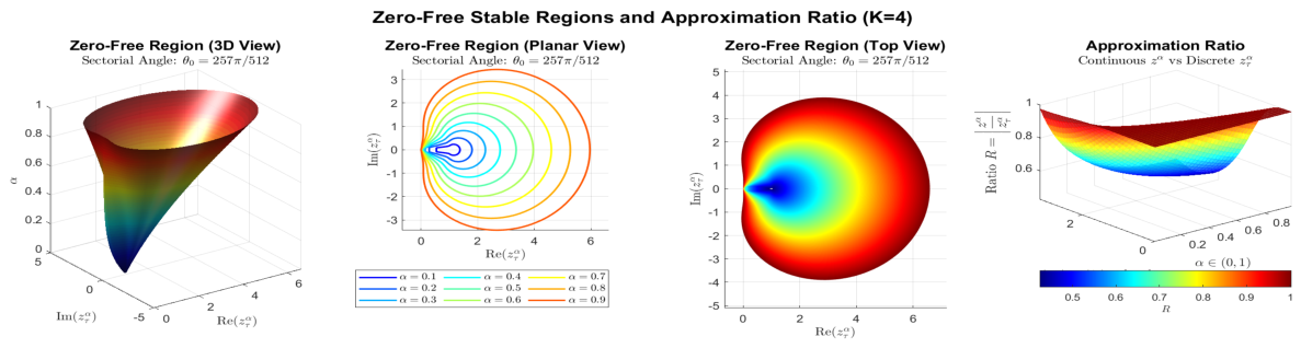
Figure 2.
Accuracy Comparison: Comparison of the Zeta scheme with the classical discrete method.
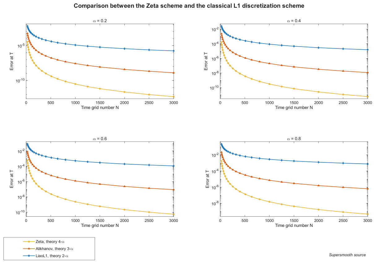
Table 1.
-norm errors and convergence rates of the unmodified higher-order Zeta schemes under the compatible condition (, ).
Table 1.
-norm errors and convergence rates of the unmodified higher-order Zeta schemes under the compatible condition (, ).
| K | Rate | ||||||||
|---|---|---|---|---|---|---|---|---|---|
| 4 | 0.1 | 6.0818e-07 | 4.0804e-08 | 2.7353e-09 | 1.8329e-10 | 1.2280e-11 | 8.2266e-13 | 5.5110e-14 | 3.8996 |
| 0.5 | 1.1635e-05 | 1.0346e-06 | 9.1690e-08 | 8.1146e-09 | 7.1768e-10 | 6.3453e-11 | 5.6091e-12 | 3.4986 | |
| 0.9 | 7.7527e-05 | 9.1063e-06 | 1.0640e-06 | 1.2419e-07 | 1.4489e-08 | 1.6902e-09 | 1.9711e-10 | 3.0991 | |
| 5 | 0.1 | 2.8818e-07 | 9.6743e-09 | 3.2436e-10 | 1.0869e-11 | 3.6412e-13 | 1.2199e-14 | 4.1009e-16 | 4.8983 |
| 0.5 | 5.5886e-06 | 2.4915e-07 | 1.1053e-08 | 4.8935e-10 | 2.1645e-11 | 9.5698e-13 | 4.2302e-14 | 4.4980 | |
| 0.9 | 3.8264e-05 | 2.2546e-06 | 1.3180e-07 | 7.6948e-09 | 4.4896e-10 | 2.6187e-11 | 1.5271e-12 | 4.0987 | |
| 6 | 0.1 | 1.7250e-07 | 2.8981e-09 | 4.8598e-11 | 8.1437e-13 | 1.3644e-14 | 2.3023e-16 | 5.3436e-18 | 5.8029 |
| 0.5 | 3.3783e-06 | 7.5576e-08 | 1.6786e-09 | 3.7179e-11 | 8.2245e-13 | 1.8184e-14 | 4.0191e-16 | 5.4973 | |
| 0.9 | 2.3764e-05 | 6.9819e-07 | 2.0450e-08 | 5.9716e-10 | 1.7423e-11 | 5.0803e-13 | 1.4663e-14 | 5.1010 | |
| 7 | 0.1 | 1.2474e-07 | 1.0494e-09 | 8.8014e-12 | 7.3755e-14 | 6.1965e-16 | 6.8723e-18 | 1.5231e-18 | 5.8720 |
| 0.5 | 2.4666e-06 | 2.7624e-08 | 3.0748e-10 | 3.4071e-12 | 3.7694e-14 | 4.1674e-16 | 4.6059e-18 | 6.4963 | |
| 0.9 | 1.7705e-05 | 2.5813e-07 | 3.8119e-09 | 5.5681e-11 | 8.1230e-13 | 1.1702e-14 | 3.0848e-17 | 6.5924 |
Table 4.
error and average convergence rate for the homogeneous problem (Example 2).
| Data Configuration | Scheme | Avg Rate | |||||||
|---|---|---|---|---|---|---|---|---|---|
| 0.1 | (I) | (A) Uncorr. | 5.07e-04 | 2.51e-04 | 1.25e-04 | 6.21e-05 | 3.10e-05 | 1.55e-05 | 1.004 |
| (B) Corr. | 5.62e-06 | 4.47e-07 | 2.23e-08 | 1.26e-09 | 7.47e-11 | 4.53e-12 | 4.147 | ||
| (II) | (A) Uncorr. | 2.32e-04 | 1.15e-04 | 5.71e-05 | 2.85e-05 | 1.42e-05 | 7.10e-06 | 1.004 | |
| (B) Corr. | 2.78e-06 | 2.05e-07 | 1.03e-08 | 5.76e-10 | 3.43e-11 | 2.08e-12 | 4.148 | ||
| 0.5 | (I) | (A) Uncorr. | 1.86e-03 | 8.94e-04 | 4.43e-04 | 2.21e-04 | 1.10e-04 | 5.50e-05 | 1.005 |
| (B) Corr. | 6.64e-04 | 2.60e-06 | 1.14e-07 | 5.50e-09 | 2.54e-10 | 9.41e-12 | 4.519 | ||
| (II) | (A) Uncorr. | 8.43e-04 | 4.06e-04 | 2.01e-04 | 1.00e-04 | 5.00e-05 | 2.50e-05 | 1.005 | |
| (B) Corr. | 2.92e-04 | 1.19e-06 | 5.29e-08 | 2.58e-09 | 1.23e-10 | 5.08e-12 | 4.461 | ||
| 0.9 | (I) | (A) Uncorr. | 9.99e-04 | 4.85e-04 | 2.33e-04 | 1.15e-04 | 5.74e-05 | 2.86e-05 | 1.021 |
| (B) Corr. | 2.11e-03 | 1.02e-05 | 9.33e-07 | 1.10e-07 | 1.29e-08 | 1.50e-09 | 3.182 | ||
| (II) | (A) Uncorr. | 4.54e-04 | 2.16e-04 | 1.04e-04 | 5.14e-05 | 2.56e-05 | 1.28e-05 | 1.020 | |
| (B) Corr. | 1.08e-03 | 4.50e-06 | 4.10e-07 | 4.83e-08 | 5.65e-09 | 6.60e-10 | 3.184 |
Table 5.
error and average convergence rate for smooth sources (Example 3).
| Data Configuration | Scheme | Avg Rate | |||||||
|---|---|---|---|---|---|---|---|---|---|
| 0.1 | (I) | (A) Uncorr. | 5.13e-05 | 2.53e-05 | 1.26e-05 | 6.28e-06 | 3.14e-06 | 1.57e-06 | 1.004 |
| (B) Corr. | 5.68e-07 | 4.52e-08 | 2.26e-09 | 1.27e-10 | 7.55e-12 | 4.58e-13 | 4.147 | ||
| (II) | (A) Uncorr. | 4.55e-04 | 2.25e-04 | 1.12e-04 | 5.58e-05 | 2.79e-05 | 1.39e-05 | 1.003 | |
| (B) Corr. | 3.32e-06 | 3.24e-07 | 1.61e-08 | 9.05e-10 | 5.36e-11 | 3.25e-12 | 4.152 | ||
| 0.5 | (I) | (A) Uncorr. | 1.88e-04 | 9.04e-05 | 4.48e-05 | 2.23e-05 | 1.11e-05 | 5.56e-06 | 1.005 |
| (B) Corr. | 6.71e-05 | 2.63e-07 | 1.16e-08 | 5.56e-10 | 2.56e-11 | 9.53e-13 | 4.519 | ||
| (II) | (A) Uncorr. | 1.67e-03 | 8.02e-04 | 3.98e-04 | 1.98e-04 | 9.90e-05 | 4.95e-05 | 1.005 | |
| (B) Corr. | 5.56e-04 | 1.81e-06 | 7.29e-08 | 2.95e-09 | 8.30e-11 | 2.57e-12 | 4.857 | ||
| 0.9 | (I) | (A) Uncorr. | 1.01e-04 | 4.90e-05 | 2.35e-05 | 1.16e-05 | 5.80e-06 | 2.89e-06 | 1.021 |
| (B) Corr. | 2.13e-04 | 1.03e-06 | 9.43e-08 | 1.11e-08 | 1.30e-09 | 1.52e-10 | 3.182 | ||
| (II) | (A) Uncorr. | 8.97e-04 | 4.37e-04 | 2.09e-04 | 1.03e-04 | 5.15e-05 | 2.57e-05 | 1.021 | |
| (B) Corr. | 1.77e-03 | 1.07e-05 | 9.80e-07 | 1.14e-07 | 1.32e-08 | 1.54e-09 | 3.189 |
Table 6.
error and average convergence rate for compatibility tests (Example 4).
| Data Configuration | Scheme | Avg Rate | |||||||
|---|---|---|---|---|---|---|---|---|---|
| 0.1 | (I) | (A) Uncorr. | 6.08e-07 | 4.08e-08 | 2.74e-09 | 1.83e-10 | 1.23e-11 | 8.22e-13 | 3.900 |
| (B) Corr. | 6.08e-07 | 4.08e-08 | 2.74e-09 | 1.83e-10 | 1.23e-11 | 8.22e-13 | 3.900 | ||
| (II) | (A) Uncorr. | 5.08e-04 | 2.51e-04 | 1.25e-04 | 6.21e-05 | 3.10e-05 | 1.55e-05 | 1.004 | |
| (B) Corr. | 5.01e-06 | 4.06e-07 | 1.96e-08 | 1.07e-09 | 6.24e-11 | 3.71e-12 | 4.185 | ||
| 0.5 | (I) | (A) Uncorr. | 1.16e-05 | 1.04e-06 | 9.17e-08 | 8.11e-09 | 7.18e-10 | 6.35e-11 | 3.498 |
| (B) Corr. | 1.16e-05 | 1.04e-06 | 9.17e-08 | 8.11e-09 | 7.18e-10 | 6.35e-11 | 3.498 | ||
| (II) | (A) Uncorr. | 1.87e-03 | 8.95e-04 | 4.43e-04 | 2.21e-04 | 1.10e-04 | 5.50e-05 | 1.006 | |
| (B) Corr. | 6.52e-04 | 1.57e-06 | 2.27e-08 | 2.61e-09 | 4.64e-10 | 5.41e-11 | 3.706 | ||
| 0.9 | (I) | (A) Uncorr. | 7.75e-05 | 9.11e-06 | 1.06e-06 | 1.24e-07 | 1.45e-08 | 1.69e-09 | 3.099 |
| (B) Corr. | 7.75e-05 | 9.11e-06 | 1.06e-06 | 1.24e-07 | 1.45e-08 | 1.69e-09 | 3.099 | ||
| (II) | (A) Uncorr. | 1.08e-03 | 4.94e-04 | 2.34e-04 | 1.15e-04 | 5.74e-05 | 2.86e-05 | 1.027 | |
| (B) Corr. | 2.19e-03 | 1.93e-05 | 2.00e-06 | 2.34e-07 | 2.74e-08 | 3.19e-09 | 3.140 |
Table 7.
error and average convergence rate for low-regularity data (Example 5).
| Data Configuration | Scheme | Avg Rate | |||||||
|---|---|---|---|---|---|---|---|---|---|
| 0.1 | (I) | (A) Uncorr. | 6.79e-07 | 1.61e-07 | 3.76e-08 | 8.79e-09 | 2.05e-09 | 4.79e-10 | 2.098 |
| (B) Corr. | 6.79e-07 | 1.61e-07 | 3.76e-08 | 8.79e-09 | 2.05e-09 | 4.79e-10 | 2.098 | ||
| 0.5 | (I) | (A) Uncorr. | 1.06e-07 | 3.76e-08 | 9.87e-09 | 1.99e-09 | 3.72e-10 | 6.76e-11 | 2.280 |
| (B) Corr. | 1.06e-07 | 3.76e-08 | 9.87e-09 | 1.99e-09 | 3.72e-10 | 6.76e-11 | 2.280 | ||
| 0.9 | (I) | (A) Uncorr. | 4.11e-07 | 2.63e-08 | 3.65e-09 | 4.40e-10 | 5.15e-11 | 5.97e-12 | 3.026 |
| (B) Corr. | 4.11e-07 | 2.63e-08 | 3.65e-09 | 4.40e-10 | 5.15e-11 | 5.97e-12 | 3.026 |
Table 8.
Observed convergence rates of Scheme A for (Example 6).
| 0.5 | 1.488 | 1.196 | 0.719 |
| 1.0 | 1.984 | 1.657 | 1.153 |
| 1.5 | 2.454 | 2.044 | 1.213 |
| 2.0 | 2.121 | 2.609 | 2.272 |
| 2.5 | 4.436 | 3.543 | 3.132 |
| 3.0 | 3.886 | 3.541 | 3.174 |
| 3.5 | 3.916 | 3.513 | 3.115 |
| 4.0 | 3.900 | 3.499 | 3.100 |
| 4.5 | 3.886 | 3.485 | 3.085 |
| 5.0 | 3.872 | 3.471 | 3.071 |
| (target) | 3.9 | 3.5 | 3.1 |
Table 9.
Absolute errors and convergence rates for (Example 7).
| Scheme | Rate | ||||||
|---|---|---|---|---|---|---|---|
| Zeta () | 0.1 | 2.83e-06 | 2.10e-07 | 1.05e-08 | 5.90e-10 | 3.50e-11 | 4.08 |
| 0.5 | 2.99e-04 | 1.22e-06 | 5.42e-08 | 2.64e-09 | 1.25e-10 | 5.30 | |
| 0.9 | 1.10e-03 | 4.62e-06 | 4.20e-07 | 4.96e-08 | 5.79e-09 | 4.38 | |
| Gao | 0.1 | 8.71e-06 | 8.50e-07 | 9.41e-08 | 1.11e-08 | 1.34e-09 | 3.17 |
| 0.5 | 4.50e-05 | 3.76e-06 | 3.38e-07 | 2.81e-08 | 1.78e-09 | 3.66 | |
| 0.9 | 1.37e-04 | 1.27e-05 | 3.35e-06 | 8.12e-07 | 1.92e-07 | 2.37 | |
| Cao | 0.1 | 4.36e-06 | 1.97e-07 | 9.73e-09 | 5.23e-10 | 2.35e-10 | 3.54 |
| 0.5 | 2.58e-04 | 1.10e-06 | 4.71e-08 | 2.12e-09 | 2.53e-10 | 4.99 | |
| 0.9 | 1.09e-03 | 4.82e-06 | 4.36e-07 | 5.10e-08 | 6.57e-09 | 4.33 |
Disclaimer/Publisher’s Note: The statements, opinions and data contained in all publications are solely those of the individual author(s) and contributor(s) and not of MDPI and/or the editor(s). MDPI and/or the editor(s) disclaim responsibility for any injury to people or property resulting from any ideas, methods, instructions or products referred to in the content. |
© 2026 by the authors. Licensee MDPI, Basel, Switzerland. This article is an open access article distributed under the terms and conditions of the Creative Commons Attribution (CC BY) license (http://creativecommons.org/licenses/by/4.0/).
Copyright: This open access article is published under a Creative Commons CC BY 4.0 license, which permit the free download, distribution, and reuse, provided that the author and preprint are cited in any reuse.