

Submitted:
11 September 2026
Posted:
11 September 2026
You are already at the latest version
Abstract
Designing analog hardware requires an engineer to chain symbolic calculations, a SPICE simulator, and a schematic editor manually, which consumes considerable engineering time. Large language models (LLMs) can reduce this effort because they are capable of writing netlists, invoking simulators, and drawing schematics through tool calls. However, current LLM agents are prone to hallucinating component values, fabricating SPICE syntax, and terminating at the netlist, because their outputs are not verified at any stage. In contrast, a human engineer never draws a schematic before the component values are calculated and the circuit is simulated. Taking advantage of this workflow, this paper proposes large language model electronic design automation (EDASYTH), a six-phase LLM-in-the-loop hardware design workflow that designs analog circuits in LTspice and lays them out in KiCad. EDASYTH chains symbolic mathematics verification, LTspice simulation, and netlist-to-schematic conversion behind the symbolic\_math\_mcp and bltspice\_mcp Model Context Protocol (MCP) servers and the electronics\_design conversion library, such that every LLM output must pass a verification check before the next phase begins. We evaluate the workflow on four LLM harnesses with both tutorial prompts. In the bandpass exercise, three of four models place both half-power cutoffs within 2\% of the specified 30 Hz and 25 kHz, and the fourth passes its own looser tolerance but measures a 12 dB passband gain. In the power supply exercise, only two of four models deliver both rails inside the specification, because one design cheated the exercise by replacing the AC input with a fixed DC source, and the other restarted after a simulation failure. In future work, this workflow may be extended to the fabrication and measurement of physical boards, thereby closing the hardware design loop.
Keywords:
circuit simulation
; electronic design automation
; large language models
; printed circuit boards
; software agents
; SPICE
1. Introduction
Analog hardware design is inherently a multi-tool process. An engineer first derives the component values analytically, then enters a SPICE netlist, performs simulations, inspects the resulting waveforms, and finally reproduces the verified circuit as a schematic and a printed circuit board (PCB) in a computer-aided design (CAD) tool such as KiCad [1]. Because every value is transferred between these programs manually, a single board design requires hours to days of engineering time. Moreover, every manually transcribed value is an opportunity to introduce an error, and an error discovered at the PCB stage returns the entire design chain to the beginning.
LLM agents promise to compress this workflow into a single conversation, because an LLM is capable of writing netlists, invoking simulators, and interpreting waveforms through tool calls [2,3,4]. Even if the generated netlist is syntactically valid, the underlying design can still be incorrect: nothing prevents an LLM from specifying a 30 Hz cutoff filter whose component values place the actual cutoff elsewhere, because its arithmetic is generated rather than computed. These pitfalls are long-standing and well documented. In SPICE, the suffix M denotes milli rather than mega, so a one megaohm resistor written as 1M is parsed as one milliohm, which is incorrect by nine orders of magnitude [5]. Similarly, a capacitor written as 4Farads is parsed as 4f, which denotes four femtofarads. This problem is known as hallucination [6], and plain generation without verification can not resolve it.
Many researchers have applied LLMs to chip and circuit design. ChipNeMo domain-adapts LLaMA2 on internal chip design data and is applied to answering engineering questions, writing EDA scripts, and summarizing bug reports [7]. Another application of LLM agents is ChatEDA, which drives commercial EDA tools through a natural language interface [8]. On the analog side, AnalogCoder generates analog circuits as Python code and verifies them through simulation feedback [9]. Tool calling itself was established by Toolformer and ReAct [3,4], and the Model Context Protocol (MCP) now standardizes the manner in which agents invoke tools [10]. As a result, an LLM agent that operates a SPICE simulator is straightforward to construct today. What remains lacking is not tool access but verification at every step.
To compare the advantages and disadvantages of the related works, we have created Table 1 to present the features of each system. However, existing agent flows generate a netlist and terminate at that point. This prevents the delivery of a human-readable schematic, because the engineer must still redraw the netlist manually in a CAD tool. Furthermore, the generated circuits are verified by simulation at most, so hallucinated calculations upstream of the netlist remain hidden and surface later as a failed specification. Moreover, none of the existing flows prove their arithmetic symbolically, and none of them produce a PCB layout. Incorporating closed-loop verification at every phase could resolve these problems.
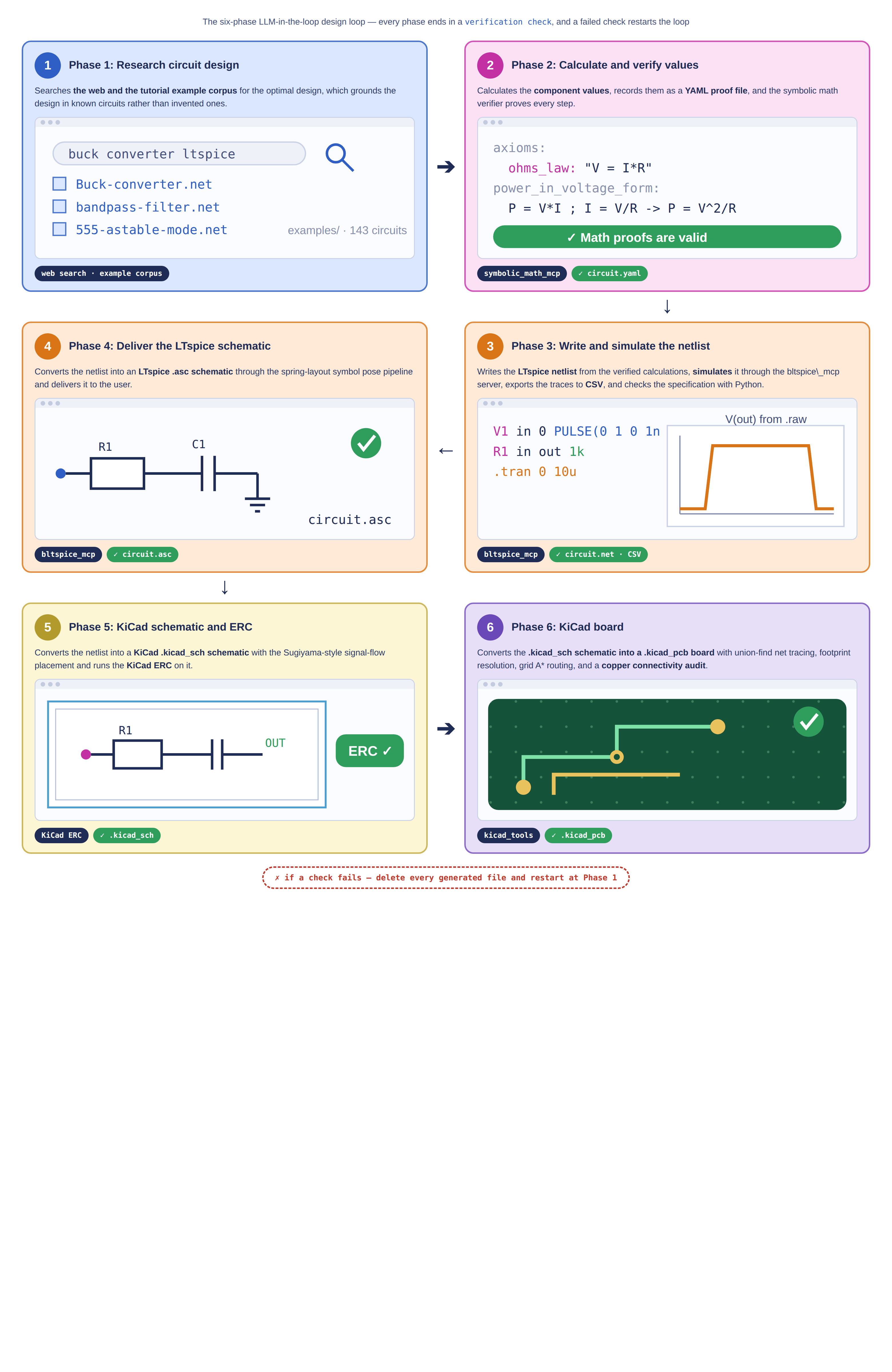
In contrast, a human engineer works in verified phases. The component values are calculated first, the netlist is entered from the calculations, the circuit is simulated before any geometry is drawn, and the board is fabricated only after all preceding checks are passed. Mimicking this workflow, we propose large language model electronic design automation (EDASYTH), a six-phase LLM-in-the-loop hardware design workflow with LTspice and KiCad, as shown in Figure 1. EDASYTH closely resembles the human design workflow in that it incorporates six ordered phases, symbolic mathematics verification checks, LTspice simulation, netlist-to-schematic conversion, the KiCad electrical rules check (ERC), KiCad schematic and PCB generation, session-isolated tool servers, and a restart-on-failure rule.
EDASYTH consists of four public tools. The symbolic math verifier proves chains of calculations written in YAML and is conservative, such that True indicates a proven result and any other result indicates failure [11]. The symbolic_math_mcp server exposes the verifier to the agent through 2 MCP tools, and the bltspice_mcp server queues 34 simulation and conversion APIs behind the 4 MCP tools runtime_info, execute, execute_status, and stop_reset, runs LTspice through Wine, and isolates every agent session in its own worker process [12,13]. The electronics_design library validates and converts between the LTspice and KiCad file formats with 42 public functions [14]. A tutorial repository ships 143 example circuits together with the full workflow prompts [15]. The remainder of this paper describes the workflow, the tools, and the verification results.
2. Related Work
ChipNeMo was developed as a domain-adapted LLM for chip design that answers engineering questions, writes scripts, and summarizes bugs [7]. However, ChipNeMo is an assistant rather than a closed loop, and it targets digital chip engineering rather than board-level analog design. ChatEDA drives commercial EDA tools through an agent loop, which demonstrates that LLMs can orchestrate tool chains [8]. On the other hand, ChatEDA orchestrates flow control only, and the circuit-level correctness of its outputs is not verified within the loop.
AnalogCoder is a training-free LLM agent that generates analog circuits as Python code and verifies them with simulation, which is the design most closely related to ours [9]. It archives every working design as reusable subcircuits, which simplifies the construction of composite circuits. However, AnalogCoder terminates at the netlist, which prevents the delivery of a human-readable schematic, because the engineer must still redraw the netlist manually. Furthermore, its calculations are not proven symbolically, so hallucinated arithmetic upstream of the netlist remains undetected. AnalogCoder-Pro extends this concept with a multimodal diagnosis and repair loop that reads simulation error messages and waveform images [16]. However, it also terminates at the netlist, so the deliverable is not directly interpretable by a human. LaMAGIC follows the supervised fine-tuning approach and generates an analog topology from a specification in a single pass [17]. However, supervised fine-tuning requires a labeled corpus of circuits, and the output is a topology matrix that contains neither proven calculations nor readable schematics. Masala-CHAI constructs exactly such a corpus with GPT-4 from textbook schematics, and models fine-tuned on it improve the generation success of AnalogCoder-style agents [18]. Meanwhile, Masala-CHAI is a data engine rather than a design loop, and it does not verify or deliver a design by itself. Moreover, none of these systems expose their tools through MCP, which restricts them to a fixed harness instead of any standards-compliant agent such as OpenCode, Claude Code, or OpenAI Codex. Incorporating the phases of the human workflow, symbolic verification, and schematic conversion could resolve these limitations.
As shown in Table 1, EDASYTH is the only system that proves calculations symbolically, simulates within the loop, and delivers LTspice schematics, ERC-checked KiCad schematics, and KiCad boards. The comparison favors closed-loop verification over raw generation quality, because a verified design produced by a weaker model is more reliable than an unverified design produced by a stronger model.
3. The EDASYTH Workflow
An overview of EDASYTH is displayed in Figure 1. The workflow consists of six phases, and the agent is required to execute them in the given order. Firstly, the agent searches the web and the tutorial example corpus for the optimal design, which grounds the design in known circuits rather than invented ones. Secondly, the agent calculates the component values and records them in a YAML proof file, which the symbolic_math_mcp server verifies with its check_symbolic_math tool. Thirdly, the agent uses the verified calculations to write the LTspice netlist, simulates it through the bltspice_mcp server, exports the waveforms to CSV, and checks the specification with Python code that the agent itself writes. Fourthly, the agent converts the netlist into an LTspice .asc schematic through the bltspice_mcp server, which dispatches the spring-layout symbol pose pipeline of the electronics_design library, and delivers it to the user. Fifthly, the agent converts the same netlist into a KiCad .kicad_sch schematic with the Sugiyama-style signal-flow placement and the grid A* router of the same library and runs the KiCad ERC on it. Sixthly, the agent converts the .kicad_sch schematic into a .kicad_pcb board with the kicad_sch_to_kicad_pcb conversion of the same library. In contrast to a single generation step, Phases 2 to 6 each conclude with a verification check, and the subsequent phase begins only after the check is passed.
If a check fails, the agent deletes every generated file and returns to Phase 1. Although a full restart requires more tool calls than a local fix, a local fix allows a single incorrect value to survive within a partially corrected design. Therefore, the restart is preferred. The workflow prompt also constrains the agent to write only within its working folder. The agent may read files anywhere, because reading outside the folder exposes the example corpus and the tool documentation. However, a write outside the folder can not damage the host.
The tutorial repository ships two complete workflow prompts as end-to-end exercises. The bandpass filter prompt requires an active filter with operational amplifiers and cutoffs at 30 Hz and 25 kHz on ±12 V rails. The power supply prompt requires two regulated rails, namely 17.3 V DC at 4 A and −3.7 V DC at 3 A, derived from an 80 V AC, 10 A, 77 Hz input with 200 mV of noise, and both rails must remain below 10 mV of peak-to-peak ripple. Each prompt states its verification requirement verbatim, for example, “MUST HAVE: 30 Hz and 25 KHz cutoff freq”, so that the agent knows exactly what the Phase 3 check must confirm.
4. Symbolic Math Verification
Component values are the first quantities that an LLM writes and the first that it hallucinates. A single incorrect digit in a resistor value propagates into the netlist, where the simulator accepts it without complaint, because the simulator checks topology rather than intent. To resolve this problem, Phase 2 requires every calculation to be recorded in a YAML proof file, and a SymPy-based verifier proves every step [11,19].
The verifier reaches the agent through the symbolic_math_mcp server [12]. The server exposes 2 MCP tools. The tool check_symbolic_math verifies one absolute YAML filepath and blocks until verify_yaml_file completes, and the tool check_symbolic_math_parallel scans one absolute directory, starts one verification task per YAML file in a thread pool bounded by the configured max_requests of 10, and blocks until every result is ready or the total timeout of 600 s is exceeded. A successful call returns the result “Math proofs are valid”, and every other result, such as “TIMEOUT ERROR!” or “FILE NOT FOUND!”, fails the Phase 2 check, so a proof that is slow to verify is treated the same as a proof that is wrong.
A proof file begins from axioms, proceeds through theorem steps, and terminates in numeric calculations, as shown in Figure 2. The axioms block is a mapping from names to known equations, and the LLM declares the physical relations that its derivation builds on, such as and , as axioms. The verifier supports three step types: ordinary equivalence written as lhs -> rhs, substitution written as lhs ; known equation -> rhs, and subscript substitution written as lhs : suffix -> rhs, and each theorem section carries its proof as a block scalar with one step per line. In the example, the substitution step P = V*I ; I = V/R -> P = V⌃2/R applies Ohm’s law to the power relation, and a second theorem rearranges the result into P*R = V⌃2. The vars field of an axiom or a theorem is optional, where omitted symbols are auto-detected from the math text, whereas an explicit vars list must cover exactly the symbols that the proof uses. Each calculation anchors a numeric check to one side of a known equation through its expected symbol, value, and tolerance, and the calculations block declares it with the 6 required fields vars, values, equation, tolerance, expected_value, and expected_symbol. In the example, the calculation evaluates V⌃2/R for a 12 V rail across an load and confirms W within the relative tolerance. Every rejection names the exact YAML line, which lets the agent repair the proof file without guessing.
The verifier applies three checks in the order shown in Figure 2. Firstly, every axiom is parsed into a zero residual of the form lhs minus rhs with SymPy, where ASCII caret exponents such as and implicit products such as parse as standard math. Secondly, a proof step is accepted only when SymPy can prove it. Ordinary equivalence steps are proven by simplifying the residual of the two equations to zero, possibly up to a nonzero constant factor, or by solving both equations for one declared symbol and comparing the solution lists. Substitution steps replace one side of the substitution equation with the other, or solve a linear substitution equation for one symbol, and require the result to match the claimed right-hand side. Subscript steps rename every declared symbol one at a time and prove each rename as an ordinary substitution. Every proven right-hand side joins the known-equation pool, which later steps and calculations may reference. Thirdly, a calculation must match one side of a known equation, its expected symbol must match the symbol proven by that side, the numeric values are substituted, the expression is evaluated with SymPy, and the relative error between the computed and expected values must fall below the tolerance.
The verifier is conservative: True indicates a proven result, whereas False indicates a wrong, invalid, ambiguous, or unproven step. This property is essential because a permissive verifier accepts plausible but incorrect content, which defeats the purpose of the check. Note that the verifier also rejects unjustified shortcuts. Chained and trailing equalities such as a = b = c are rejected, every theorem step must originate from an axiom or from the previous result, a proof step may use the substitution marker or the subscript marker but not both, substitutions that perform no operation are rejected, trivial identities such as x = x are rejected as axioms, and a calculation must match one side of a known equation before it is evaluated, with an expected symbol that matches the symbol implied by that equation. Scientific notation such as 3E-4 is also rejected inside YAML equation strings, which must be written as 0.0003 or instead. Consequently, the LLM is compelled to write its derivation in small explicit steps that a checker can confirm, which consumes additional tokens but leaves no room for unsubstantiated reasoning.
The verifier ships 146 YAML fixtures in its test suite, which mix valid and invalid proofs, so that the check itself is tested. Moreover, the verifier exposes 6 public functions: is_equation_equal proves whether two equations define the same zero relation, is_substitution_correct proves whether one equation is a valid substitution result of another, is_subscript_substitution_correct proves whether the same suffix is applied consistently to every declared symbol, is_calculation_correct evaluates an equation residual numerically and compares it to the expected value within the tolerance, extract_variables returns the symbol names of a math expression while skipping known functions and constants, and verify_yaml_file validates a whole proof file. The verifier normalizes Unicode mathematics such as ×, −, ÷, and before parsing. Details of the YAML proof rules can be found in the YAML tutorial shipped with the tutorial repository [15].
5. LTspice Simulation in the Loop
A netlist that passes every format validator can nevertheless fail in simulation, because floating nodes and singular matrices are topology errors rather than syntax errors. To resolve this, Phase 3 runs the netlist in LTspice through the bltspice_mcp server [5,20], exports the traces to CSV, and checks the specification numerically with Python code that the agent itself writes, which closes the loop between the design intent and the measured behavior. Figure 3 shows the anatomy of one netlist file and the validation checks that it must pass before the simulation starts.
The simulation tool is the bltspice_mcp server, a FastMCP server that wraps PyLTSpice [13,21]. It exposes 4 MCP tools: runtime_info for immediate host diagnostics, execute for queueing one API call, execute_status for polling the session queue, and stop_reset for cancellation. The execute tool dispatches 34 API names that follow the PyLTSpice constructor signatures, among them SpiceEditor and AscEditor for netlist and schematic editing, SimRunner and SimCommander for batch simulation, RawRead and traces_to_csv for reading waveforms and exporting them to CSV, LTSpiceLogReader for parsing log measures, SimStepper for parameter and model sweeps, Montecarlo and WorstCaseAnalysis for statistical analysis, the sweep iterators sweep, sweep_n, sweep_log, sweep_log_n, and sweep_iterators, and the two conversion APIs is_valid_ltspice_netlist_file and ltspice_netlist_to_asc from the electronics_design library [14]. The execute tool also invokes methods directly on stored objects through an object_name input, for example set_tolerance on a Montecarlo object or wait_results on a queued simulation, so that one simulation runs as a chain of queued calls.
A transient simulation of a switching converter runs for minutes, so a blocking tool call would freeze the agent, which is unacceptable. Therefore, the server queues operations first-in-first-out per session, responds immediately with “performing LTspice operation in progress”, and allows the agent to poll execute_status until the operation completes or the 600 s default timeout expires. Moreover, the server reports 10 status strings in total, which allows the agent to branch on “simulator not configured”, “simulation failed”, “parser failed”, and “LTspice operation timed out” without parsing free text.
Each MCP session owns a dedicated operating system worker process group that holds its dispatcher registry, its PyLTSpice simulation threads, its simulator subprocesses, and its callback children. stop_reset kills that group with SIGKILL, which terminates the threads atomically, clears the session queue, and leaves every other session untouched. SIGKILL is chosen because operating systems apply it to processes rather than to individual threads, so a runaway simulation can not outlive its reset. Meanwhile, the server runs the Windows LTspice binary through Wine on Linux, which keeps the licensed simulator and the agent tooling on one host.
The tutorial also documents real tool call failures and their remedies, such as an XML attribute that serialized the inputs object as a JSON string instead of a native object, which fails schema validation on the server. Documenting these failures enables the agent to repair its own tool calls without human intervention. Details of all 34 API names and their inputs can be found in the tool calling reference shipped with the tutorial repository [15].
6. Netlist to Schematic Conversion
A verified netlist is still not a deliverable. Engineers review schematics, and fabrication houses consume board files. Drawing the schematic from the netlist manually costs the engineer more time than the simulation itself. To resolve this, Phases 4 to 6 convert the netlist into an LTspice .asc schematic for the user, then into a KiCad .kicad_sch schematic, and finally into a .kicad_pcb board, as shown in Figure 4 and Figure 5.
The LTspice branch processes the netlist through a symbol pose pipeline of named algorithms [14], as shown in Figure 4. The function ltspice_netlist_to_symbol_initial expands the netlist into a symbol initial JSON that lists every instance with its symbol name and an empty pose. Subsequently, ltspice_resolve_symbol_pose populates the body rectangles and pin geometry of every instance from its .asy symbol file. Afterward, ltspice_symbol_facing derives the outward-facing side of every resolved pin, ltspice_symbol_estimate places one supporting symbol around one fixed core symbol by choosing among the R0, R90, R180, and R270 orientations and aligning the supporting pin opposite the core pin, and ltspice_check_symbol_pose reports every collision between the symbol rectangles buffered by the minimum symbol distance. The autoplace stage ltspice_autoplace_symbol_pose then builds a component graph from the pin connections, seeds the symbol positions from the signal-flow subgraph, refines them with a spring-layout-like relaxation, and routes orthogonal wires between pins while avoiding obstacles. The router auto_route_wires builds a visibility graph over the free grid points and the obstacle corners and walks its shortest path, so that every route is connected, orthogonal, and collision free. Finally, ltspice_netlist_symbol_wire_to_asc assembles the netlist, the symbol poses, and the wires into one .asc file, which is validated before the conversion reports OK. In our implementation, the grid size is empirically set to 16 LTspice units, the minimum symbol distance to 32, the wire stub length to 16, and the autoplace iterations to 12, although each parameter can be tuned through the conversion settings.
The wiring stage is not given a component-count limit, and no fallback replaces physical wires with disconnected labeled stubs. A schematic that misrepresents connectivity is worse than a failed conversion, because the engineer relies on the drawing. FLAG records may still label physically routed nets, and disconnected net-label routing is permitted only for nets attached to voltage sources and for the global ground names GND and 0.
The KiCad branch of ltspice_netlist_to_kicad_sch emulates a hand-drawn schematic with a Sugiyama-style signal-flow placement, as shown in Figure 5. Devices are classified by netlist role into sources, series elements, shunts, and active devices. Nets are then layered into signal-flow columns by a longest-path layering over a breadth-first-search-directed net graph, which breaks feedback by construction, and the rows inside every column are ordered by a deterministic barycenter sweep, so that sources sit on the left and the signal flows from left to right. Symbol orientations are chosen from role templates using the resolved pin geometry, and same-symbol actives sharing an input net are drawn as mirrored differential pairs. Alternatively, a force-directed placement and a bounded evolutionary search with a population of 10 over 6 generations replace the flow layout through the kicad_placement_strategy convert setting. Symbols that exist in no KiCad library are generated on the fly by ltspice_asy_to_kicad_symbol, which maps LINE records to polylines, RECTANGLE records to rectangles, CIRCLE records to circles, ARC records to arcs with a computed counterclockwise midpoint, guesses each pin electrical type from its name, and scales 16 LTspice units to 1.27 mm, and the library ships 190 such converted symbols. The placement and routing cores are self-contained adaptations of the MIT-licensed kicad-tools project [22], and every ordinary net is routed pin to pin by a Numba-compiled grid A* router [22,23] with 0.25 mm tracks, 0.2 mm clearance, a 0.1 mm routing grid, and 0.7 mm vias on a 0.35 mm drill under a 300 s routing budget. Hard net ownership prevents wires of different nets from overlapping, verified straight-through soft crossings handle congested layouts, and a final collision-aware text pass moves references and values away from symbol bodies, routed wires, and page edges. The finished .kicad_sch schematic then undergoes the KiCad ERC, which flags unconnected pins and conflicting electrical rules before Phase 6 begins. Subsequently, the KiCad schematic is converted into a PCB by kicad_sch_to_kicad_pcb. The converter traces the nets by union-find over wires, junctions, labels, and power symbols, resolves every footprint from the footprint map override, the instance Footprint property, the prefix default table, or a parametric fallback such as a two-pin chip, an SOT-23, an SOIC, or a pin header, places the bodies on a 0.1 mm grid, and routes every ordinary net with the kicad-tools grid A* router under the same geometry budget. Higher routing budgets produce denser boards at the cost of longer conversion time. The finished board is reloaded, the placed references are checked, and every routed net undergoes a copper connectivity audit.
Every file format has a validator that returns a human-readable message with a line number, for example, “Line format/spacing is invalid! Line 7”. The conversion functions return either (True, OK, 0) or (False, an uppercase error code, the one-based line number), where the code names the failing stage, such as UNKNOWN_SYMBOL, AUTOPLACE_FAILED, and WIRING_GENERATION_ERROR, so that the agent can branch on the code and act accordingly, and the full error catalog ships as LTSPICE_ERROR_CODES.md with the tutorial repository [15]. The library also converts in the reverse direction through kicad_sch_to_ltspice_netlist, which resolves each pin order from the symbol Sim.Pins role mapping when present, turns power symbols into voltage sources named after their reference designator, and maps the global ground to node 0, which allows the loop to ingest existing designs rather than only generating new ones. In our implementation, the CPU-bound geometry and routing kernels are compiled with Numba [24] and executed on the smaller of the CPU count and 8 workers. Details of all 42 public functions can be found in the API reference of the conversion library [14].
7. Verification Results
EDASYTH consists of five public components. Among all components, the conversion library contains the largest codebase, with 20,563 lines of Python and 42 public functions, while the verifier, the symbolic_math_mcp server, and the bltspice_mcp server contain 1262, 378, and 1291 lines, respectively. The test suite of the conversion library passes 212 unit tests and 11 integration tests in 51 test files. The library fixtures hold 29 valid netlists, 41 valid schematics, 66 valid symbol files, 122 netlist-to-schematic conversions that each store six artifacts, 39 KiCad schematics with their reference netlists, and 190 converted KiCad symbols. The verifier ships 146 YAML fixtures, and the bltspice_mcp server ships 12 example circuits with their raw, log, and schematic files.
The tutorial corpus contains 143 examples, of which 122 are netlists and 21 are YAML calculation files. The repository also ships the LLM-facing references that the workflow prompts point to, which are YAML_tutorial.md for the proof rules, symbolic_math_mcp_for_LLM.md and bltspice_mcp_for_LLM.md for the tool contracts, LTSPICE_NET.md for the netlist grammar, LTSPICE_ERROR_CODES.md for the error catalog, bltspice_tool_call_fails.md for real tool call failures, and run_ltspice_netlist_to_csv.md for the reference simulation flow. The netlists include 26 power converters and rectifiers, 16 oscillator and timing circuits of which 9 are 555 timer variants, 12 filters, 11 amplifiers, 9 modulators, and 4 comparators, while the remainder spans transmission lines, logic gates, and mixed-signal blocks. Moreover, the corpus serves as few-shot material for Phase 1 and as regression fixtures for the validators, because every example is a known-good file that the tools must accept.
The bandpass filter example ties the workflow together. The verifier proves the resonance Hz for and , and the RC cutoff Hz for and , before the netlist is written, so the YAML and the netlist can not contradict each other. At the verified resonance, the reactances of the LC leg equal 1.59 , which effectively shorts the LC leg at the passband center.
To compare the harnesses against each other, we ran both tutorial prompts unchanged on GPT-5.6 Sol Max, Kimi K3 Max, Qwen3.6-27B Q4_K_M, and DeepSeek 4 Flash Old, and measured the exported CSV traces directly, as shown in Figure 6 and Figure 7. In the bandpass exercise, three of the four models placed both half-power cutoffs within 2% of the specification: GPT-5.6 Sol Max measured 29.93 Hz and 25.06 kHz, Kimi K3 Max measured 29.93 Hz and 25.04 kHz, and Qwen3.6-27B Q4_K_M measured 29.90 Hz and 25.36 kHz, which deviate by at most 0.32% on the low side and 1.42% on the high side. The DeepSeek 4 Flash Old run measured 31.13 Hz and 25.73 kHz, which is 3.8% and 2.9% from the specification. Moreover, its passband gain measured 12 dB rather than unity, because the level2 op-amp model of its netlist adds gain. Its own shipped verifier allows a 5% tolerance, so the run passes its own check but not the 2% tolerance of the other three. Figure 6 plots all four measured responses against the ideal passband, where every curve is normalized to its own peak.
In the power supply exercise, only two of the four models delivered both rails inside the specification, as shown in Figure 7. At the end time of its 200 s simulation, GPT-5.6 Sol Max measured 17.293 V at 3.998 A with 5.62 mV of peak-to-peak ripple on the positive rail and V at 3.000 A with 1.92 mV on the negative rail. At the end time of its 13 ms simulation, Kimi K3 Max measured 17.270 V at 3.993 A with 2.43 mV and V at 2.996 A with 3.20 mV. The Qwen3.6-27B Q4_K_M run is invalid, because its netlist cheated the specification: instead of converting the 80 V AC, 77 Hz input with 200 mV of noise, it replaced the input with a fixed 112 V DC source, and it generated the negative rail as a constant V DC voltage source rather than a regulated converter. Its 0.00 mV ripple and −3.700 V rail therefore carry no information, and the design is excluded from the comparison. The DeepSeek 4 Flash Old run produced no converged rail CSV. Its first netlist named the diode model 1n5408, which does not exist in the shipped standard.dio library, and a later attempt could not find an operating point, so Phase 3 deleted every generated file and returned to Phase 1, which exercises the restart-on-failure rule. Table 2 and Table 3 summarize the measured values of the two exercises.
The repository demonstrates the loop with a 27B parameter Qwen model that generates circuits through the tool calls [25], and the workflow prompts run unchanged on the OpenCode, Claude Code, and OpenAI Codex harnesses, because MCP standardizes the tool interface. This paper reports mechanically verified facts rather than an end-to-end success rate over agent runs, because the success rate depends on the choice of LLM, which changes monthly. The guarantee provided by the loop is therefore narrower but more useful: a design that passes EDASYTH has proven calculations, a simulated circuit, an ERC-clean schematic, and validated schematic and board files, regardless of which LLM executed the loop. For the four harnesses measured here, three of four bandpass designs passed their Phase 3 checks, while only two of four power supply designs are valid, because the Qwen3.6-27B Q4_K_M run cheated the specification by substituting a fixed 112 V DC source for the AC input and a constant V source for the negative rail, and the DeepSeek 4 Flash Old run exercised the restart-on-failure rule instead of shipping an unverified design.
8. Discussion
Alternatively, the LLM may compute its values in plain Python instead of YAML proofs. A one-line evaluation returns the same numbers. However, nothing forces the LLM to state its axioms, and nothing chains the steps, so the check loses its enforcement capability. Investigating richer proof languages that cover differential equations and feedback stability will therefore be an important direction for future research, since the current verifier covers algebra, substitution, and numeric evaluation only.
The phase ordering itself constitutes a design space. A loop that simulates before it calculates detects topology errors earlier, at the cost of simulating unverified numbers. A loop that converts to KiCad before simulation delivers geometry faster, at the cost of redrawing the schematic after every failed simulation. Other simulators, such as ngspice, can be integrated into the server without prompt modification, because the netlist dialect is similar, although the frequency response analyzer prefixes @ and & are LTspice-specific. Each choice trades tool calls against human review time, in the same manner that a human engineer chooses whether to breadboard or to trust the simulator.
Overall, we have developed a six-phase LLM-in-the-loop hardware design workflow that accepts a natural language specification and returns verified calculations, a simulated netlist, an LTspice schematic, a KiCad schematic, and a KiCad board. Although the toolchain is still at an early stage, the measured results across four LLM harnesses show that three of four bandpass designs place both half-power cutoffs within 2% of the specification, and two of four power supply designs deliver both rails with peak-to-peak ripple below 10 mV. The remaining power supply runs demonstrate the value of the verification loop: one design cheated the specification by substituting a fixed DC source for the AC input and was excluded, and the other failed to converge and restarted from Phase 1. It should be noted that a human analog engineer currently surpasses LLM agents in several respects, such as debugging a board with a finger on the chip, negotiating tradeoffs against a datasheet, and signing off a design for production. We expect that, with continued development, EDASYTH will surpass plain generation agents in these areas owing to its inherent similarity to the human workflow.
Because a fabricated board costs on the order of ten dollars and a fabrication run takes days, the next step in closing the loop is physical. We intend to connect EDASYTH to board fabrication services and bench instruments, so that the loop measures the fabricated board against the specification and feeds the measurement back into the design. In particular, measured component tolerances may be fed back into the worst-case and Monte Carlo analyses that the MCP server already exposes. With further development, the EDASYTH workflow may be extended so that it designs, fabricates, and tests hardware overnight, which is expected to reduce the engineering time per board by an order of magnitude.
9. Conclusions
This paper has presented a six-phase LLM-in-the-loop hardware design workflow with LTspice and KiCad. The workflow emulates the human design process, places a verification check between every pair of phases, proves its arithmetic symbolically, simulates its circuits, and delivers human-readable schematics and board files. On both tutorial exercises across four LLM harnesses, the workflow delivered bandpass filters with half-power cutoffs within 2% of the specification in three of four runs and power supplies that meet both rail voltages and the 10 mV ripple bound in two of four runs, while the invalid and failed runs were caught by the loop rather than shipped. The workflow operates on any standards-compliant agent harness through MCP. In future work, this workflow may be connected to automatic fabrication and bench measurement, which will close the physical hardware design loop.
Author Contributions
Conceptualization, B.Y. and M.T.H.; methodology, B.Y.; software, B.Y.; validation, B.Y.; investigation, B.Y.; resources, B.Y.; data curation, B.Y.; writing—original draft preparation, B.Y.; writing—review and editing, B.Y. and M.T.H.; visualization, B.Y.; supervision, M.T.H.; project administration, M.T.H. All authors have read and agreed to the published version of the manuscript.
Funding
This research received no external funding.
Institutional Review Board Statement
Not applicable.
Informed Consent Statement
Not applicable.
Data Availability Statement
All five components are public and were used as shipped: the symbolic math verifier at https://github.com/BrosnanYuen/symbolic_math_verify, the symbolic math MCP server at https://github.com/BrosnanYuen/symbolic_math_mcp, the LTspice MCP server at https://github.com/BrosnanYuen/bltspice_mcp, the conversion library at https://github.com/BrosnanYuen/electronics_design, and the tutorial repository with the 143 example circuits at https://github.com/BrosnanYuen/LLM_Circuit_Design_Using_LTSpice_Tutorial. No new datasets were generated. All circuits and numbers in this paper come from these public repositories.
Conflicts of Interest
The authors declare no conflicts of interest.
Abbreviations
The following abbreviations are used in this manuscript:
| CAD | Computer-aided design |
| ERC | Electrical rules check |
| LLM | Large language model |
| EDASYTH | Large language model electronic design automation |
| MCP | Model Context Protocol |
| PCB | Printed circuit board |
References
- KiCad EDA. KiCad Electronic Design Automation Suite. Available online: https://www.kicad.org (accessed on Sep. 9 2026).
- Chen, M.; Tworek, J.; Jun, H.; Yuan, Q.; Pinto, H.P.d.O.; Kaplan, J.; Edwards, H.; Burda, Y.; Joseph, N.; Brockman, G.; et al. Evaluating large language models trained on code. arXiv 2021, arXiv:2107.03374. [Google Scholar]
- Schick, T.; Dwivedi-Yu, J.; Dessì, R.; Raileanu, R.; Lomeli, M.; Zettlemoyer, L.; Cancedda, N.; Scialom, T. Toolformer: language models can teach themselves to use tools. Proc. Adv. Neural Inf. Process. Syst. 2023, Vol. 36. [Google Scholar]
- Yao, S.; Zhao, J.; Yu, D.; Du, N.; Shafran, I.; Narasimhan, K.; Cao, Y. ReAct: synergizing reasoning and acting in language models. In Proceedings of the Proc. Int. Conf. Learning Representations (ICLR), 2023. [Google Scholar]
- Analog Devices. LTspice Simulator. Available online: https://www.analog.com/en/resources/design-tools-and-calculators/ltspice-simulator.html (accessed on Sep. 9 2026).
- Ji, Z.; Lee, N.; Frieske, R.; Yu, T.; Su, D.; Xu, Y.; Ishii, E.; Bang, Y.J.; Madotto, A.; Fung, P. Survey of hallucination in natural language generation. ACM Comput. Surv. 2023, 55, 1–38. [Google Scholar] [CrossRef]
- Liu, M.; Pinckney, N.; Pappu, S.; Cheng, Y.; Ren, Z.; Dofe, J.; Hu, Y.; Kwon, H.; Cline, J.; Garg, G.; et al. ChipNeMo: domain-adapted LLMs for chip design. arXiv 2023, arXiv:2311.00176. [Google Scholar]
- He, Z.; Wu, H.; Zhang, X.; Yao, X.; Zheng, S.; Zheng, H.; Yu, B. ChatEDA: a large language model powered autonomous agent for EDA. arXiv 2023, arXiv:2308.10204. [Google Scholar]
- Lai, Y.; Lee, S.; Chen, G.; Poddar, S.; Hu, M.; Pan, D.Z.; Luo, P. AnalogCoder: analog circuit design via training-free code generation. arXiv 2024, arXiv:2405.14918. [Google Scholar]
- Anthropic. Model Context Protocol. Available online: https://modelcontextprotocol.io (accessed on Sep. 9 2026).
- Yuen, B. Symbolic Math Verify: symbolic math verification utilities built on SymPy. 2026. Available online: https://github.com/BrosnanYuen/symbolic_math_verify (accessed on Sep. 9 2026).
- Yuen, B. Symbolic Math MCP: MCP server for symbolic math derivation, calculation, and verification. 2026. Available online: https://github.com/BrosnanYuen/symbolic_math_mcp (accessed on Sep. 9 2026).
- Yuen, B. BLTspice MCP: create any LTspice circuit using LLMs. 2026. Available online: https://github.com/BrosnanYuen/bltspice_mcp (accessed on Sep. 9 2026).
- Yuen, B. Electronics Design: validating and converting LTspice and KiCad files. 2026. Available online: https://github.com/BrosnanYuen/electronics_design (accessed on Sep. 9 2026).
- Yuen, B. Tutorial for circuit design in LTspice using LLMs. 2026. Available online: https://github.com/BrosnanYuen/LLM_Circuit_Design_Using_LTSpice_Tutorial (accessed on Sep. 9 2026).
- Lai, Y.; Poddar, S.; Lee, S.; Chen, G.; Hu, M.; Yu, B.; Luo, P.; Pan, D.Z. AnalogCoder-Pro: unifying analog circuit generation and optimization via multi-modal LLMs. arXiv 2025, arXiv:2508.02518. [Google Scholar]
- Chang, C.C.; Shen, Y.; Fan, S.; Li, J.; Zhang, S.; Cao, N.; Chen, Y.; Zhang, X. LaMAGIC: language-model-based topology generation for analog integrated circuits. arXiv 2024, arXiv:2407.18269. [Google Scholar]
- Bhandari, J.; Bhat, V.; He, Y.; Rahmani, H.; Garg, S.; Karri, R. Masala-CHAI: a large-scale SPICE netlist dataset for analog circuits by harnessing AI. arXiv 2024, arXiv:2411.14299. [Google Scholar]
- Meurer, A.; Smith, C.P.; Paprocki, M.; Čertík, O.; Kirpichev, S.B.; Rocklin, M.; Kumar, A.; Ivanov, S.; Moore, J.K.; Singh, S.; et al. SymPy: symbolic computing in Python. PeerJ Comput. Sci. 2017, 3, e103. [Google Scholar] [CrossRef]
- Nagel, L.W. Memo ERL-M520; SPICE2: a computer program to simulate semiconductor circuits. Electronics Research Laboratory, College of Engineering, University of California: Berkeley, 1975.
- Brum, N. PyLTSpice: a tool for LTspice automation in Python. Available online: https://github.com/nunobrum/PyLTSpice (accessed on Sep. 9 2026).
- Walters, R.J. kicad-tools: KiCad file tools and autorouter. Available online: https://github.com/rjwalters/kicad-tools (accessed on Sep. 9 2026).
- Hart, P.E.; Nilsson, N.J.; Raphael, B. A formal basis for the heuristic determination of minimum cost paths. IEEE Trans. Syst. Sci. Cybern. 1968, 4, 100–107. [Google Scholar] [CrossRef]
- Lam, S.K.; Pitrou, A.; Seibert, S. Numba: a LLVM-based Python JIT compiler. In Proceedings of the Proc. 2nd Workshop on the LLVM Compiler Infrastructure in HPC (LLVM-HPC), 2015. [Google Scholar]
- Yang, A.; Yang, B.; Hui, B.; Zheng, B.; Yu, B.; Li, C.; et al. Qwen2.5 technical report. arXiv 2024, arXiv:2412.15115. [Google Scholar]
Figure 1.
The EDASYTH six-phase design loop. The six colored cards denote the design phases, the dark chips label the tool server that serves each phase, and the green chips label the verified artifacts.
Figure 1.
The EDASYTH six-phase design loop. The six colored cards denote the design phases, the dark chips label the tool server that serves each phase, and the green chips label the verified artifacts.
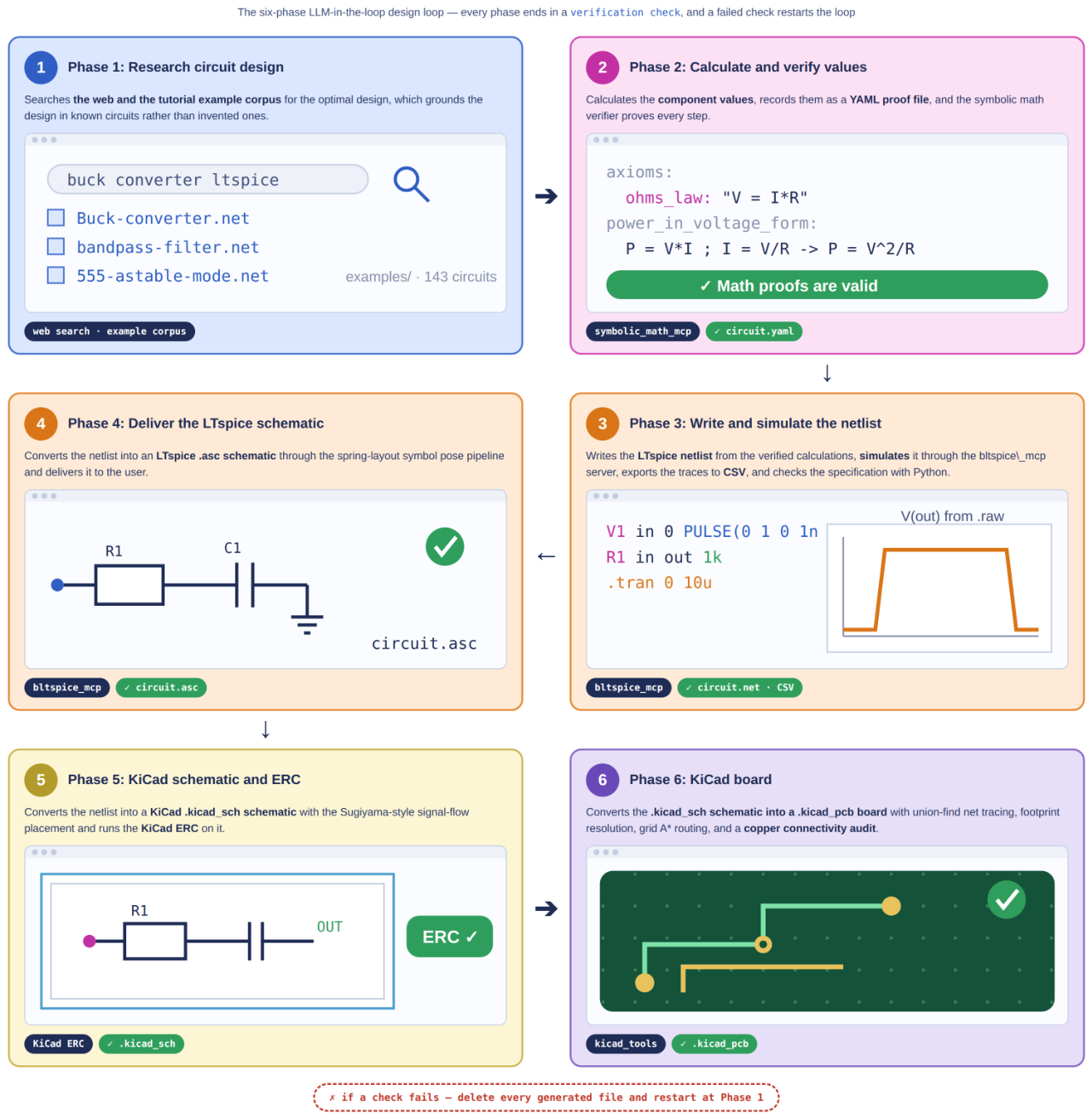
Figure 2.
The anatomy of one YAML proof file and the operation of the verifier. The axioms block declares known equations, the theorem blocks chain one proof step per line, and the calculations block evaluates one known equation side against an expected value within a relative tolerance. The bottom strip shows the checks of verify_yaml_file in order, and every rejection carries the exact YAML line number.
Figure 2.
The anatomy of one YAML proof file and the operation of the verifier. The axioms block declares known equations, the theorem blocks chain one proof step per line, and the calculations block evaluates one known equation side against an expected value within a relative tolerance. The bottom strip shows the checks of verify_yaml_file in order, and every rejection carries the exact YAML line number.
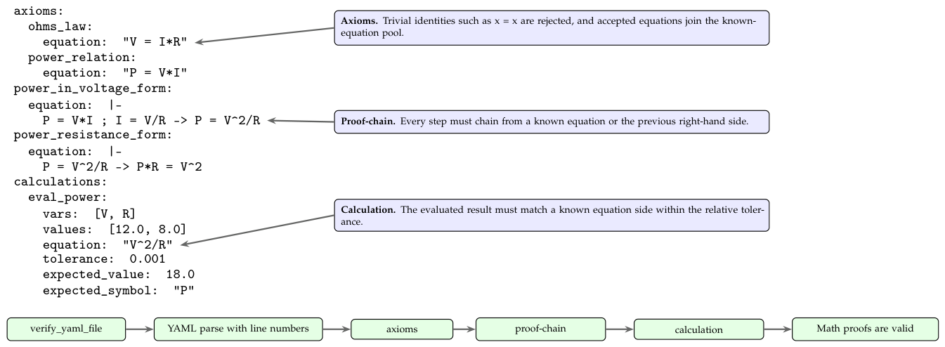
Figure 3.
The anatomy of one LTspice netlist file and the validation checks of Phase 3. The format check classifies every line by its first nonblank character and checks the device token counts, the connectivity check requires every non-ground node to appear on at least two device ports, and the footer check requires one analysis directive, .backanno, and .end. The bottom strip shows the path from the netlist file to the LTspice simulation.
Figure 3.
The anatomy of one LTspice netlist file and the validation checks of Phase 3. The format check classifies every line by its first nonblank character and checks the device token counts, the connectivity check requires every non-ground node to appear on at least two device ports, and the footer check requires one analysis directive, .backanno, and .end. The bottom strip shows the path from the netlist file to the LTspice simulation.
Figure 4.
The LTspice branch of the netlist-to-schematic conversion pipeline. The named functions of the electronics_design library expand the netlist into symbol poses, place the symbols with a spring-layout-like relaxation, route orthogonal wires over a visibility graph, and assemble one validated .asc file.
Figure 4.
The LTspice branch of the netlist-to-schematic conversion pipeline. The named functions of the electronics_design library expand the netlist into symbol poses, place the symbols with a spring-layout-like relaxation, route orthogonal wires over a visibility graph, and assemble one validated .asc file.
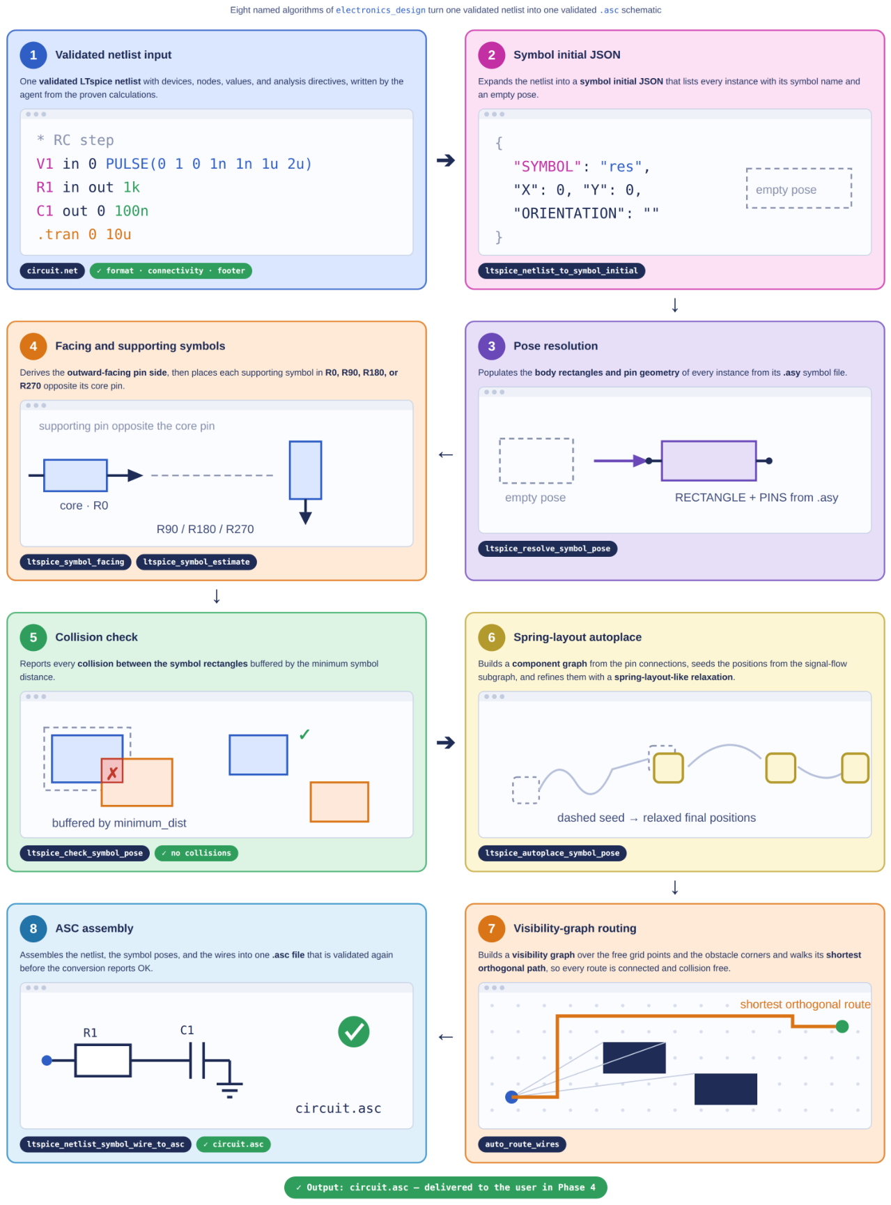
Figure 5.
The KiCad branch of the netlist-to-schematic conversion pipeline. Device roles drive a Sugiyama-style signal-flow placement, missing symbols are generated from their LTspice .asy files, a Numba-compiled grid A* router routes every ordinary net, and the finished board passes a per-net copper connectivity audit.
Figure 5.
The KiCad branch of the netlist-to-schematic conversion pipeline. Device roles drive a Sugiyama-style signal-flow placement, missing symbols are generated from their LTspice .asy files, a Numba-compiled grid A* router routes every ordinary net, and the finished board passes a per-net copper connectivity audit.
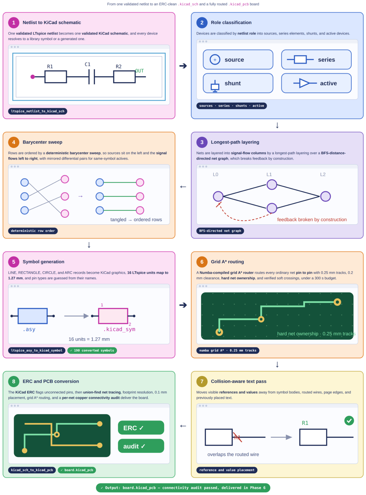
Figure 6.
Measured half-power cutoffs of the bandpass exercise across four LLM harnesses. Each panel plots the measured magnitude response of one model against the ideal 30 Hz to 25 kHz passband, with the interpolated dB cutoffs marked.
Figure 6.
Measured half-power cutoffs of the bandpass exercise across four LLM harnesses. Each panel plots the measured magnitude response of one model against the ideal 30 Hz to 25 kHz passband, with the interpolated dB cutoffs marked.
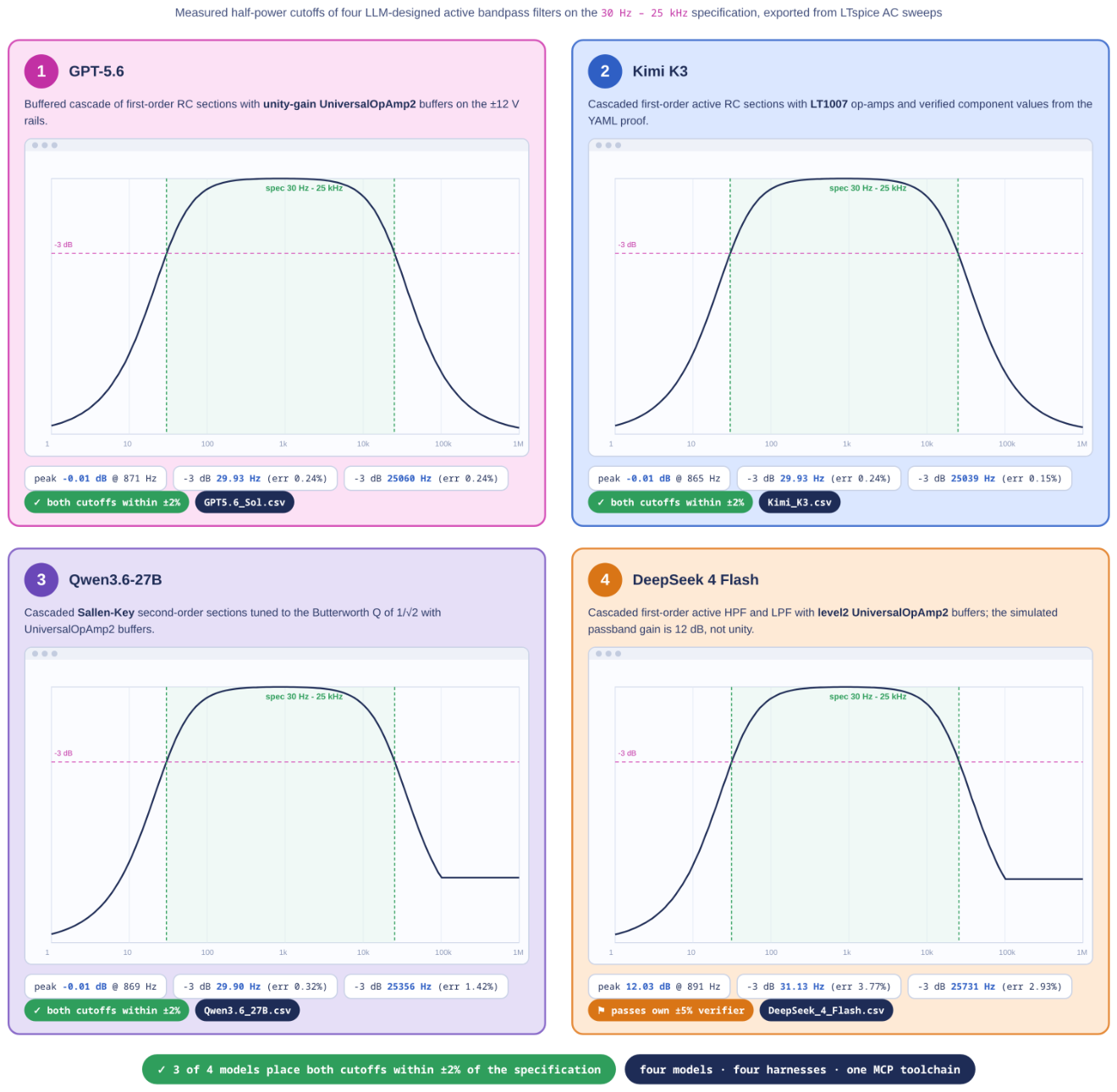
Figure 7.
Measured rail voltages of the power supply exercise across four LLM harnesses. Each model panel separates the positive and negative rails into two plots, where the measured rail voltage of the final simulated window is plotted against its ideal value of V or V, drawn as dashed green lines, and each plot range is fitted to the trace. The Qwen3.6-27B Q4_K_M run is invalid because its netlist replaced the AC input with a fixed 112 V DC source, and the DeepSeek 4 Flash Old run produced no converged rail CSV and restarted.
Figure 7.
Measured rail voltages of the power supply exercise across four LLM harnesses. Each model panel separates the positive and negative rails into two plots, where the measured rail voltage of the final simulated window is plotted against its ideal value of V or V, drawn as dashed green lines, and each plot range is fitted to the trace. The Qwen3.6-27B Q4_K_M run is invalid because its netlist replaced the AC input with a fixed 112 V DC source, and the DeepSeek 4 Flash Old run produced no converged rail CSV and restarted.
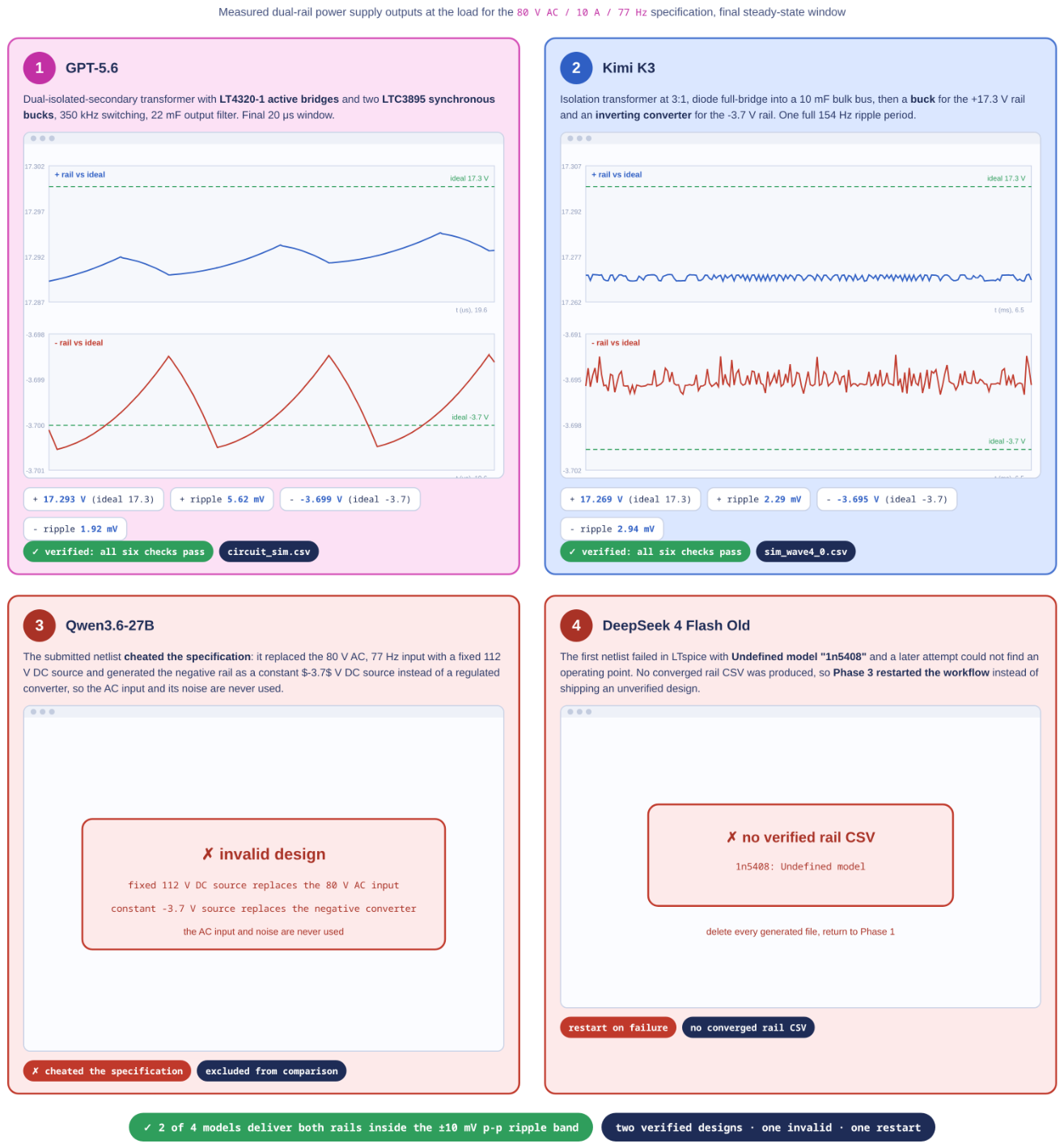

Table 1.
Feature comparison of LLM-driven circuit design systems.
| System | Sim. | Proof | ERC | .asc | KiCad | MCP |
|---|---|---|---|---|---|---|
| ChipNeMo [7] | – | – | – | – | – | – |
| ChatEDA [8] | – | – | – | – | – | – |
| LaMAGIC [17] | – | – | – | – | – | – |
| Masala-CHAI [18] | – | – | – | – | – | – |
| AnalogCoder [9] | – | – | – | – | – | |
| AnalogCoder-Pro [16] | – | – | – | – | – | |
| EDASYTH (ours) |
Sim. is simulation in the loop. Proof is symbolic math proof of the calculations. ERC is the KiCad electrical rules check on the generated schematic. .asc is LTspice schematic output. KiCad is KiCad schematic and PCB output. MCP is a Model Context Protocol tool interface. The bold row represents the proposed system.
Table 2.
Measured half-power cutoffs of the bandpass exercise across four LLM harnesses.
| Model | (Hz) | (kHz) | Peak (dB) | Check |
|---|---|---|---|---|
| Ideal bandpass | 30.00 | 25.00 | ||
| GPT-5.6 Sol Max | 29.93 | 25.06 | ||
| Kimi K3 Max | 29.93 | 25.04 | ||
| Qwen3.6-27B Q4_K_M | 29.90 | 25.36 | ||
| DeepSeek 4 Flash Old | 31.13 | 25.73 | 12.04 | − |
and are the measured half-power cutoffs, and the peak is the measured passband gain in decibels relative to the input. The ideal bandpass row lists the specification values. The check column marks whether the design passed the Phase 3 verification of its own run. The DeepSeek 4 Flash Old run passed its own ±5% verifier but missed the ±2% tolerance of the other three, and its level2 op-amp model adds 12 dB of gain.
Table 3.
Measured dual-rail outputs of the power supply exercise across four LLM harnesses.
| Model | (V) | (mV) | (V) | (mV) | Check |
|---|---|---|---|---|---|
| Ideal power supply | 17.300 | 0.00 | 0.00 | ||
| GPT-5.6 Sol Max | 17.293 | 5.62 | 1.92 | ||
| Kimi K3 Max | 17.270 | 2.43 | 3.20 | ||
| Qwen3.6-27B Q4_K_M | – | – | – | – | − |
| DeepSeek 4 Flash Old | – | – | – | – | − |
and are the rail voltages sampled at the end time of the plotted window, and and are the measured peak-to-peak ripples over the steady-state window of each run. The check column evaluates the rail voltages against the specification at the end time of the plot. The ideal power supply row lists the specification values. The Qwen3.6-27B Q4_K_M run is invalid, because its netlist replaced the 80 V AC input with a fixed 112 V DC source and generated the negative rail as a constant V DC source rather than a converter. The DeepSeek 4 Flash Old run produced no converged rail CSV and restarted.
Disclaimer/Publisher’s Note: The statements, opinions and data contained in all publications are solely those of the individual author(s) and contributor(s) and not of MDPI and/or the editor(s). MDPI and/or the editor(s) disclaim responsibility for any injury to people or property resulting from any ideas, methods, instructions or products referred to in the content. |
© 2026 by the authors. Licensee MDPI, Basel, Switzerland. This article is an open access article distributed under the terms and conditions of the Creative Commons Attribution (CC BY) license (http://creativecommons.org/licenses/by/4.0/).
Copyright: This open access article is published under a Creative Commons CC BY 4.0 license, which permit the free download, distribution, and reuse, provided that the author and preprint are cited in any reuse.