

Submitted:
09 September 2026
Posted:
11 September 2026
You are already at the latest version
Abstract
A (T, I, N, F) neutrosophic quadruple records support, pure indeterminacy, neutrality and refutation as four free intensities. When a panel of sources reports point quadruples and each channel is summarised by an interval, the resulting box contains combinations that no source reported, and an index that adds channels of different sources may overflow the unit although every source is consistent. For the range box, the direct overflow of the box bounds the largest per-source overflow from above, and, as the main result, the marginal ranges of any subset of channels identify the largest per-source sum only up to a sharp interval: sum of lower bounds plus the largest width at one end, sum of upper bounds at the other, every value between them being realisable. The classification of a box by its upper corner into six overflow types is proved to be a partition. A closed-form overflow probability, 1/72 per source under a stated generative model, anchors a simulation in which, for twenty independent sources under the scaled model, range boxes flag a direct overflow in 99% of panels while 25% contain an overflowing source. Panel diagnostics and a reference implementation accompany the results.
Keywords:
neutrosophic set
; interval-valued quadruple
; paraconsistency
; partial identification
; marginalisation
; multi-source evidence
; conflict index
; order statistics
; multi-source artificial intelligence
; retrieval-augmented generation
1. Introduction
The (T, I, N, F) neutrosophic set of Smarandache [1] refines the indeterminacy channel of a neutrosophic set [2] into two channels: pure indeterminacy , the part of a judgement that rests on information which is missing or cannot be evaluated, and neutrality , the part that rests on evidence which is present but favours neither the proposition nor its negation. In that definition each of , , , may be a single value or a subset of , and the only constraint is the trivial one, . The interval case, in which each channel is a closed subinterval of , is thus already covered by that definition; the contribution of this paper is the analysis of what an interval-valued quadruple retains when it is built channel by channel from a panel of point reports, and of how the per-source information can be recovered from it.
The problem is concrete. Let sources (experts, retrieved documents, annotators, model instances) each report a point quadruple about a proposition . The natural interval summary of the panel takes, in each channel, the range of the reports. The resulting box contains the point , which combines the strongest support of one source with the strongest refutation of another. If the sum exceeds 1, a reader of the box sees a direct overflow although no source may have reported one. Conversely, a box built from quantiles rather than ranges can hide a source whose own report overflows. The box has lost the dependence between channels within a source, and Ahmad [3] has recently shown, for set-valued quadruples in general, that marginal bounds cannot identify the dependence structure among the four components. This paper takes the next step and quantifies what marginal bounds do identify.
This situation is now common in artificial intelligence pipelines: a language model receives several retrieved passages that disagree, an ensemble of model instances returns divergent judgements, or a crowd of annotators splits on an item. In each case the system must decide whether it faces a source whose own evidence overflows, sources that are polarised against one another, missing information or balanced evidence. The (T, I, N, F) representation records the first, third and fourth per source as free intensities; polarisation is a property of the panel, and it is read by comparing the panel’s box with its sources. The results below say what survives of that distinction when the panel is summarised by intervals.
The contributions are the following.
- 1.
- A sharp partial-identification theorem (Section 6). If a box is the exact range box of a finite panel, then for any non-empty subset of channels the largest per-source sum over lies between and , where are the bounds of the box; both ends and every value between them are attained by panels with that range box, and we give sufficient numbers of sources for each construction. For the polar pair this yields an identified interval for the largest per-source direct overflow. In particular a range box may force the existence of an overflowing source even though its lower corner does not overflow, a situation that the earlier notion of “necessary” overflow cannot express.
- 2.
- A clean separation between what a box says about one point and what it says about all points (Section 4). The six overflow types (Consistent, Strong, Weak I, Weak II, Mixed, Very Weak) are defined on the upper corner of the box and proved to partition the space of boxes. They are a classification of boxes, not an enumeration of the types of their points; universally quantified statements are handled by separate flags, and the set of types realised inside a box is characterised by exact feasibility conditions on its bounds (the types of its corners do not suffice).
- 3.
- A reproducible simulation with an analytic anchor (Section 9). Under a stated generative model the probability that a single source overflows is exactly , so the share of panels with an overflowing source is . This closed form validates the simulator, which then reports, with Monte Carlo error, how often the range box and the interquartile box flag a direct overflow, how often they do so falsely with respect to the per-source flag, and how the picture changes when sources are normalised or dependent.
- 4.
- Corrected diagnostics (Section 10). A state classification of panels that distinguishes absence of overflow, per-source overflow below or above a threshold, and box excess without per-source overflow; an influence measure on the direct box index that does not blame a source for widening the indeterminacy channel; and a revision procedure whose only guarantee is termination.
The semantic apparatus (an elicitation protocol that makes and distinct, the convention that the unit is the overflow threshold, and an auxiliary lattice with the two negations that the literature has proposed) is kept to what the results require, and each convention is labelled as such. Everything numerical in the paper is produced by a reference implementation whose tests reproduce every example and every table.
2. Related Work and Delimitation
Four-component neutrosophic sets. Quadripartitioned single-valued neutrosophic sets [4] split indeterminacy into contradiction and unknown components; their interval-valued form was introduced by Pramanik [5], who defined containment, the complement , intersection and union and proved their set-theoretic properties, and was continued by Bag and Pramanik [6] with the symmetric difference, convexity, and truth- and false-favourite sets. Those works are set-theoretic; they do not consider panels of sources, sums of channels or the dependence between channels. The (T, I, N, F) set [1] uses a different split, pure indeterminacy versus neutrality, and its components may be subsets of ; the version of that paper available from the author’s repository (accessed 9 September 2026) also fixes negation as , treats as a positive quality in its score and accuracy functions, and defines conjunction and disjunction with -norms applied to and -conorms to or the reverse. Ahmad [3] develops the set-valued case through its componentwise infima and suprema: the total envelope width is the sum of the four channel widths, refinement contracts the envelope, and, as a non-identifiability principle, marginal envelope information cannot determine whether the components are independent, partially dependent or totally dependent. The present paper adopts his bound notation, does not re-derive those facts, and answers the quantitative question his principle leaves open: given exact marginal ranges of a panel, which values of the largest per-source sum are possible? Ahmad’s TINF-Consensus [7] aggregates annotator responses into a quadruple in which is a derived polarisation measure; the of the present paper is a free intensity of inconclusive evidence elicited per source (Section 3.2), so the two models share the vocabulary but not the coordinates. The ladder of strong, weak and very weak paraconsistency for point quadruples was stated in [8]; Section 4 refines its weak regime into three disjoint types and lifts the ladder to boxes.
Interval and graded models. Interval-valued intuitionistic fuzzy sets [9,10] are the closest classical ancestor, with the normalisation that the present model drops. Interval neutrosophic sets [11] fix a lattice convention on which Section 7 comments, and Rivieccio [12] examined its logical prospects and problems, including the behaviour of the complement on indeterminacy. Interval arithmetic [13] supplies the elementary lemma of Section 4. The dependence between neutrosophic components was made explicit by Smarandache [14].
Conflict and evidence. In Dempster–Shafer theory [15,16] on the frame , the pair , satisfies , the belief–plausibility interval being ; the transferable belief model [17] and DSmT [18] carry conflict as a separate mass rather than as an overflow of singleton masses. Subjective logic [19] represents an opinion by belief, disbelief and uncertainty summing to one, which distinguishes ignorance from balanced evidence ; a distribution over four labels can also separate neutrality from indeterminacy. The comparison made here is therefore narrow: a normalised model cannot represent a source-level excess together with two free non-polar intensities, and it is that combination which the overflow analysis needs. Possibility theory [20] and credal sets [21] motivate reading a box as a set of admissible points, and the identification results of Section 6 are in the spirit of partial identification in statistics [22]: the data (marginal ranges) determine a set of values of the target (the largest per-source sum), not a point.
Disagreement in data. Annotator disagreement is signal rather than noise [23,24], and reliability can be estimated by latent-class models [25]; knowledge conflicts between retrieved passages are studied in retrieval-augmented generation [26]; conflicting laboratory interpretations of the same genomic variant are recorded in ClinVar [27]. These settings supply panels of the kind analysed here; none is used as data in this paper.
What is claimed, and against what. The contribution is the exact identification region of Theorem 1, its sharpness (both ends and every interior value are attained by explicit constructions, with sufficient numbers of sources), and its use for reading boxes built from panels (Example 1, the states of Section 10). The ingredients are elementary, and the statement holds for any finite family of bounded vectors; we regard that generality as an asset for use rather than a weakness. The point of comparison is precise. Interval arithmetic [13] bounds a sum over a box by , and that lower end is all that the box as a set can give. A range box carries one more piece of information, that each bound is attained by some source, and Theorem 1 shows that this raises the lower end to and that nothing more can be extracted. The lower-bound argument itself is not new: coordinatewise bounds of the form “one range at its maximum, the others at their minima” occur in scheduling, for instance as the first inequality in Equation (8) of Ravi and Tunçel [28], and we claim no priority for it. What is characterised here is the inverse problem: given only exact marginal ranges and a panel of arbitrary finite size, the complete set of compatible values of the largest per-source sum, with constructions for its endpoints and every interior value. Partial identification [22] supplies the vocabulary of an identification region, not this characterisation. The non-identifiability principle of [3] states that marginal bounds cannot recover the dependence structure; Theorem 1 states exactly what they do recover about the largest per-source sum.
What is not claimed. The definition of an interval-valued quadruple, the additivity of widths, and the qualitative loss of dependence under marginalisation are prior work. No consequence relation is defined, so no logic is proposed. No empirical validation is reported.
3. Representation and Semantics
3.1. Interval-Valued Quadruples
Let be a universe of discourse. A (T, I, N, F) neutrosophic set on [1] assigns to each four components that are non-empty subsets of . Throughout, channels are written in the fixed order and ranges over .
Definition 1 (interval-valued quadruple). An interval-valued (T, I, N, F) element is a quadruple of closed intervals
with lower bound , upper bound and width . The box of is , and a selection is a point . An interval-valued (T, I, N, F) set on assigns such an element to every ; since every statement below concerns a single , the argument is suppressed.
Definition 1 is the interval case of the set-valued definition of [1]; degenerate intervals recover single-valued quadruples. The total width equals the width of the envelope [3, Theorem 3.2], and is the imprecision ratio. Whether width means the imprecision of one source or the dispersion of a panel depends on how the element was constructed (Section 6.1).
3.2. Elicitation Protocol for I Versus N
Both and are free coordinates in ; the distinction between them is fixed by the protocol under which a source produces its report, not by the mathematics.
Definition 2 (elicitation semantics).A source examines a body of evidence about a proposition. (i) Unit of evidence. The body is first segmented into items by a rule fixed in advance; a statement that both supports and refutesis either kept as one item or split into a supporting and a refuting item, and the rule states which. (ii) Classification. Each item is assigned to exactly one of four disjoint classes: supporting (favoured), refuting (favoured), equivocal (bears onbut favours neither side), inconclusive (bears onbut cannot be evaluated by the source). Items that do not bear onare excluded. (iii) Intensities. For each class the source reports an intensity in, how strongly the items of that class, taken together, bear on;are the intensities of the supporting, refuting, equivocal and inconclusive classes. Intensities are elicited independently; they are not shares of a unit.
Under Definition 2, measures items that are individually balanced and does not re-count the balance between supporting and refuting items, which is visible as . Because intensities are not shares, a source with strong supporting and strong refuting items reports , and a source with weak items in every class reports a sub-unit total. Both states are representable, and neither is an error.
Remark 1 (what the protocol does and does not establish).Assigning names to disjoint classes makesandoperationally distinct; it does not establish statistical identifiability or agreement between sources, and the values depend on the segmentation rule of (i). Any application must report the rule and the agreement of independent sources on the four-way classification. The expectation that new evidence of the same kind lowers(inconclusive items get resolved) and leavesunchanged (equivocal items stay equivocal) is an empirical hypothesis about sources that follow the protocol; it is stated so that it can be tested, and nothing below depends on it.
3.3. the Unit as an Overflow Threshold
Following the neutrosophic convention [2,8], a sum of channels that exceeds 1 is called an overflow, and a direct overflow. Three points must be kept in view.
- (a)
- The threshold is a convention on a cardinal scale. It presupposes that the intensities of different classes are commensurable and that 1 marks “the whole of what a consistent reporter could allocate”. The condition is not invariant under increasing reparametrisation: the report overflows, but after the monotone rescaling the same source reports , which does not. Any application must therefore fix the scale on which intensities are read.
- (b)
- A direct overflow is not by itself a logical contradiction. The paper defines no designated values and no consequence relation. The report overflows although the refuting intensity is low, while does not overflow although both sides are supported. The correspondence with the glut value of Belnap–Dunn four-valued logic [29,30] is informal and conditional on the scale; logics that reason under gluts [31,32] are complementary to the representation given here.
- (c)
- The complementary quantity , when positive, is a deficit with respect to the conventional threshold. Because intensities are not additive masses, it is not a probability of “missing evidence”; it records that the four classes together bear weakly on . Section 5.3 gives its interval form.
4. Overflow of a Box: Possible and Necessary Readings
For non-empty write for the sum of the corresponding coordinates of a selection.
Lemma 1 (extremes over a box).For every boxand every,
and attains every value between them.
Proof. The coordinates of a selection range independently over their intervals, so a sum is extremised term by term [13]; is continuous on the connected set , hence attains every intermediate value. Consequently a box contains a selection with if and only if (possible overflow of ), and every selection has if and only if (necessary overflow of ). The two coincide when the intervals in are degenerate. For , a direct overflow is possible but not necessary: the box contains both consistent and overflowing selections.
4.1. Six Types on the Upper Corner
Write , , and .
Definition 3 (types of a box). A box is of exactly one of the following types, tested in this order.
- Strong: .
- Weak I (indeterminacy-driven): , , .
- Weak II (neutrality-driven): , , .
- Mixed (I+II): , , .
- Very Weak: and .
- Consistent: .
Proposition 1 (partition). The six types are mutually exclusive and jointly exhaustive on the set of boxes.
Proof. If the box is Strong and satisfies no other clause. Otherwise let ; the four truth-value combinations are disjoint and exhaustive, being Mixed, Weak I and Weak II. In the case , Very Weak and Consistent are separated by whether . The reference implementation additionally verifies the partition on all quadruples of upper bounds on the grid (tests/test_ivtinf.py). The label Consistent names the condition and carries no logical claim. The ladder of [8] for point quadruples has three regimes, its weak regime being the disjunction of Weak I and Weak II; Definition 3 splits that disjunction into three disjoint cases (I only, N only, both) and applies it to boxes through the upper corner. The Mixed case is the most common non-strong outcome of range boxes with three or more sources (Section 9), which is why it receives its own label.
Remark 2 (what the type is).The type of a box is the type of its upper cornerunder the point-valued ladder. It is a classification of the box and a flag: the box admits an overflowing selection of the stated kind. It is not the set of types of the points of the box, which is generally larger, nor a statement about all of them. The Very Weak condition does not require every sub-sum to be at most 1:,is Very Weak although; the taxonomy is organised around the polar pair and asks which non-polar channel drives the excess.
4.2. Necessary Flags and Realised Types
Replacing upper by lower bounds in Definition 3 produces another partition of boxes (by their lower corner), but it is not a partition into “necessary types”: the lower-corner clause “” says that some selection is consistent, not that all are. Universally quantified statements are kept separate:
- : ; every selection has a direct overflow.
- : ; every selection overflows the unit.
- : ; every selection is consistent (equivalently, the type is Consistent).
, and excludes both. A box of any type other than Consistent for which neither nor holds contains selections of several types.
Proposition 2 (types realised inside a box).Writeand. The points of a box realise the type Strong if and only if; Consistent if and only if; Weak I if and only if,and; Weak II if and only if,and; Mixed if and only if,and; and Very Weak if and only ifand, whereis maximised over(a piecewise linear function whose maximum is attained at an endpoint or at one of the breakpoints,); when that interval is empty, as for,, Very Weak is not realised.
Proof. Every condition of Definition 3 depends on a point only through , and , and by Lemma 1 (applied to the sub-box ) ranges over independently of and . Strong needs for some ; Consistent needs , which is easiest at the three lower bounds. Weak I needs , and ; the choice , is optimal, and the condition becomes , i.e. , and . Weak II is symmetric. Mixed needs , and , i.e. . Very Weak needs , and ; for fixed the largest admissible and are and , which must be at least and , giving the stated range for and the function . The types of the sixteen corners do not suffice: for , , , the point is Weak I (, , ) while the two corners are Consistent and Mixed. The implementation applies Proposition 2 and is tested against brute-force enumeration of points. For the worked example of Section 8 the box is of type Strong and its points realise all six types.

Table 1.
Type and necessary flags of seven boxes, computed in exact rational arithmetic. The second row admits a direct overflow that is possible but not necessary. The last row has a total of exactly 1 and is Consistent.
Table 1.
Type and necessary flags of seven boxes, computed in exact rational arithmetic. The second row admits a direct overflow that is possible but not necessary. The last row has a total of exactly 1 and is Consistent.
| Type | ||||||||||
| [0.6, 0.8] | [0,0] | [0,0] | [0.5, 0.7] | 1.5 | 1.5 | 1.5 | 1.5 | Strong | yes | yes |
| [0, 0.8] | [0,0] | [0,0] | [0, 0.7] | 1.5 | 1.5 | 1.5 | 1.5 | Strong | no | no |
| [0.3, 0.4] | [0.4, 0.5] | [0,0] | [0.2, 0.3] | 0.7 | 1.2 | 0.7 | 1.2 | Weak I | no | no |
| [0.3, 0.4] | [0,0] | [0.4, 0.5] | [0.2, 0.3] | 0.7 | 0.7 | 1.2 | 1.2 | Weak II | no | no |
| [0.2, 0.4] | [0.2, 0.4] | [0.2, 0.4] | [0.2, 0.3] | 0.7 | 1.1 | 1.1 | 1.5 | Mixed | no | no |
| [0.2, 0.3] | [0.2, 0.3] | [0.2, 0.3] | [0.2, 0.3] | 0.6 | 0.9 | 0.9 | 1.2 | Very Weak | no | no |
| [0.2, 0.2] | [0.3, 0.3] | [0.1, 0.1] | [0.4, 0.4] | 0.6 | 0.9 | 0.7 | 1.0 | Consistent | no | no |
5. Overflow Indices and Deficits
5.1. Box Indices
For a box the overflow index of a channel subset is , the amount by which the largest sum over exceeds the unit. The four used in the paper are
They are ordered, , and non-decreasing in every upper bound they contain; the type of Definition 3 is a function of which of them are positive. In the Strong regime, and .
Remark 3 (normalisation and what the indices do not detect).Dividing each index by its maximum (forchannels) maps all four to, but the normalised values need not preserve the order of the raw ones (forthey are), they are not probabilities, and a single threshold across them has no justification; thresholds must be set per index. Moreover the indices measure overflow of sums that containand; they are blind to the non-polar channels on their own: the statesandhave maximal indeterminacy and neutrality respectively and all four indices equal to 0. Decisions that depend onormust read those channels directly (Section 10).
5.2. Per-Source (Joint) Indices
When the panel of point reports , , is available, the joint index of is
the largest overflow reported by a single source; is the case . Joint indices do not depend on how the box is constructed. A box index and a joint index answer different questions: “can the box’s extremes be combined into an overflow?” and “did some source itself overflow?”.
5.3. Deficits
By Lemma 1 the total of a selection lies in , which gives two deficits with respect to the unit,
the guaranteed deficit (every selection falls short of the unit by at least this amount) and the possible deficit. and are different things: is declared by the source (items that were examined and found inconclusive), is residual (all four intensities are low). Under a normalising protocol every source has , yet the panel box can have because it combines lower bounds of different sources: two normalised sources and give a range box with . This is the same marginalisation effect as in Section 6, seen from below.
6. What a Marginal Box Knows About Its Panel
6.1. Constructions
Four constructions turn a panel into an interval-valued element, and they measure different things. The range box takes in each channel; the quantile box takes of the reports ( gives the interquartile box); both record dispersion across sources. The Student and bootstrap constructions (Section 8) estimate the panel mean and narrow as grows however divided the panel is. All four treat channels separately and lose the pairing of channels within a source.
6.2. the Marginalisation Bound for the Range Box
Proposition 3 (marginalisation bound).For a non-empty finite panel and its range box, and for every non-empty,
with equality if and only if both sides are zero or a single source attains for every simultaneously.
Proof. For each , ; take the maximum over and apply the positive part, which is monotone. Equality at a positive value requires , which holds exactly when one source attains every channel maximum in . Definition 4 (marginalisation gap). For the range box, .
When no source has a direct overflow and the whole of the box index is produced by combining extremes of different sources: the panel is polarised. When , is the additional overflow obtained by combination; it is not a measure of disagreement in general (the two sources and differ by 0.4 in and have ), and three identical sources have with . For the range box, implies : the range box never misses a source-level direct overflow. Proposition 3 does not extend to other constructions: with the interquartile box, a panel of ten in which one source reports and nine report has and . For a general construction the signed difference may be negative and must not be called a gap.
Remark 4 (what the diagnostic requires of the representation).The distinction between a panel that contains a source with a direct overflow and a panel whose box overflows only by combining extremes of different sources is drawn by the pair, not byalone: the panelsandboth have, withequal toand. What the diagnostic requires is that the reportedandof a source be free to vary independently on the fixed scale: if the reported channels are constrained to be non-negative shares of a unit, the per-source direct overflowis identically zero and the box corner has a single reading, disagreement between sources (the simulation ofSection 9shows the range box of normalised sources reaching that corner in most panels of ten or more sources). Two free polar coordinates suffice for this particular diagnostic;andadd the further distinctions of Definition 2 once the direct pair is settled. The comparison fixes the meaning and the scale of the reported channels. It does not exclude normalised representations that carry conflict as an explicit state: four-valued probability assignmentswith a conflict mass [33] recover , with , so that exactly when (the recovered direct overflow is , not the conflict mass ), and the belief-mass models of Section 2 carry conflict as a separate mass. The claim is about these channels and indices: with intensities elicited as in Definition 2, the pair of indices and the identified interval of Section 6.3 separate source-level direct overflow from overflow introduced by marginal aggregation.
6.3. Sharp Partial Identification from Marginal Ranges
Proposition 3 is elementary and one-sided. The following result states exactly which values of the largest per-source sum are compatible with given marginal ranges.
Theorem 1 (partial identification of the largest per-source sum).Letbe a non-empty finite panel, letbe its range box with boundsand widths, and letbe a non-empty set of channels. Define. Then
Both bounds are sharp over the class of all non-empty finite panels, of any cardinality, whose range box is exactly : there are panels in attaining and panels attaining , and for every there is a panel in with .
Proof. Upper bound: every coordinate of every source is at most its channel maximum. Lower bound: let attain and let be a source with , which exists because is a maximum over the panel. Then , and this sum. Sharpness. Write and let be the unit vector of channel . Let be the number of non-degenerate channels and consider the panel . Its range box is : in a non-degenerate channel the point has coordinate and the point has ; in a degenerate channel every point has . When the point is redundant, since each lower bound is then attained by for any , so can be taken of size , or according as , or . Its -sums are for and for , so . The panel of the two extreme corners (a single point if is a point) has range box and . For , by Lemma 1 there is a point with and for (raise the -coordinates from towards until the sum reaches , which is possible since ); then has range box and . Corollary 1 (identified interval for the direct overflow). With and the exact ranges of a panel,
and every value in each interval is attained by some panel with these ranges.
Proof. Theorem 1 with : , and the positive part is monotone and continuous. Proposition 4 (how many sources the constructions need). Let be the number of non-degenerate channels of . The constructions of Theorem 1 attain the upper bound with two sources (one if ); the lower bound with one source if , two if and if (hence with at most sources when the channels outside are degenerate and is not a point); and an interior value with one source more than the lower construction. These are sufficient numbers, not always minimal ones. With exactly two sources and non-degenerate channels in , the only realisable values of are the -sums of a pair of complementary corners of ; in particular for with and only and occur.
Proof. The first three claims read off the constructions in the proof of Theorem 1; that one source cannot realise a box with is clear, since the range box of one source is a point. For two sources with range box , each channel bound must be attained by one of them, so in every non-degenerate channel ; hence and are complementary corners on those channels, and is the larger of their two -sums. For the two pairings give and . Example 1 (a box that forces an overflowing source). Let and be exact ranges of a panel. The lower corner has , so no necessary flag holds and the box contains consistent selections. Yet Corollary 1 gives : every panel with these ranges contains a source with . The two statements “every compatible panel contains an overflowing source” and “every point of the box overflows” are different quantifications, and only the second is captured by the flag . The lower bound is attained by the panel , the upper by , and the value by adding to the first panel; with exactly two sources only the values and occur.
Remark 5 (relation to non-identifiability of dependence).Ahmad’s principle [3, Proposition 8.1] states that quantities computed from marginal bounds cannot distinguish dependence structures. Theorem 1 is the quantitative complement: the marginal ranges of a panel do not determine, but they confine it to the interval, and nothing outside that interval is compatible with them. The width of the identified interval,, is the sum of all but the largest width in; it vanishes when at most one channel inis non-degenerate, which is the case in which the box loses no information about. In the vocabulary of partial identification [22], the range box is the observable, the target, and the identification region when the number of sources is unknown. If the number of sources is known, the identification region can be strictly smaller: for , and , the four channel maxima must be attained by three sources, so some source attains two of them and although ; the value is realised by , , . The characterisation with fixed is left open. The theorem uses no property specific to neutrosophic quadruples: it holds for any finite family of vectors with bounded coordinates and any sum of coordinates. Its content relative to interval arithmetic is the term : the box alone gives the lower end , attainment of the bounds by sources adds the largest width (an argument that also appears, in a scheduling setting, in [28]), and the constructions show that this is the whole of the information the ranges carry about . We state the result for panels of quadruples because that is where the box construction and the overflow reading arise; we are not aware of an earlier characterisation of the identified set in that setting, and the attribution is open to correction.
6.4. Large Panels
Proposition 5 (limits for independent sources).Let the sources be independent draws from a common distribution on, and letbe the essential supremum of channelandthat of. Then almost surely, as,and.
Proof. For a real random variable with essential supremum , almost surely and for every ; by the Borel–Cantelli lemma along and monotonicity of the maximum, almost surely. Apply this to , and and use continuity of . Under the two generative models of Section 9 one has in both, for normalised sources and for scaled sources, so in both models while and respectively, and the gap tends to and . The conclusion depends on the essential suprema and not on independence alone; a distribution whose is bounded by 1 has for every while its range box can still tend to a full overflow.
7. Auxiliary Algebra: Lattice, Negations and Ranking
The results above do not need an algebra on boxes; this section records, in compressed form, the structure that the (T, I, N, F) literature uses for connectives and ranking, with the precision that the two readings of require. An order on boxes is obtained by ordering each of the eight bounds and taking the product: upward and downward in every convention, downward, and either upward, as in the Smarandache orientation (S) of [1], where is a positive quality, or downward like , as in the Wang orientation (W) of interval neutrosophic sets [11]. Join and meet are the componentwise suprema and infima of bounds in the chosen order (so the channel of is , the channel , and so on); they are not set-theoretic unions and intersections of intervals, which can be empty.
Proposition 6 (lattice structure).Letbe the set of interval-valued quadruples. In either orientation,is a complete lattice (every family, the empty one included, has a supremum and an infimum) satisfying the distributive law, with top and bottom
The negation of [1] is an involution satisfying De Morgan’s laws for the orientation-S operations; the complement of the interval neutrosophic convention is an involution satisfying De Morgan’s laws for the orientation-W operations. Neither structure is Boolean.
Proof. Let and its dual, both complete distributive chains, and let be the product of eight factors, one per bound, each or according to the orientation; is a complete lattice with componentwise operations and is distributive because each factor is. is the subset of on which for each channel, and it is closed under arbitrary joins and meets of because both bounds of a channel carry the same orientation ( and likewise for infima); the empty family gives the listed top and bottom, which satisfy . Hence is a complete sublattice of and inherits distributivity. permutes factors, sending -bounds to -bounds and -bounds to -bounds; in orientation S each pair has opposite orientations, so is an order-reversing involution of preserving , and an order-reversing involution turns joins into meets. swaps and and reflects each and bound by with the two bounds exchanged, which is order-reversing on a factor of fixed orientation and preserves ; hence it is De Morgan in orientation W. For the channel of (or ) is , so neither structure is Boolean. Under Definition 2 an item that is inconclusive or equivocal about is equally so about ; the evidential complement respects this and is an involution, but it fixes the and factors, so it is order-reversing in neither orientation and fails De Morgan’s laws (for and the channel of is while that of is ). The three operations serve different purposes: , natural when is a positive quality, and , whose reflection of Rivieccio [12] discussed, carry the De Morgan structure; preserves the per-class intensities when a proposition is negated under Definition 2. None is an evidence-pooling rule; pooling is what Section 6.1 provides. The implementation checks the lattice laws and both De Morgan pairs on 3,000 random triples of boxes.
For ranking, with midpoints , the score, accuracy, extended certainty and certainty functions of [1] applied to midpoints are , , and , and on single-valued quadruples the chain is injective [1]. Because under Definition 2 is neither support for nor against , we use the family
which orders boxes as does at , penalises both non-polar channels at , and reduces to the net polarity at ; with it ranks pure indeterminacy and pure neutrality differently (for and , gives and reverses the order). is monotone for the truth order when its weights have the sign of the orientation ( in W; in S). Ranking lexicographically by with the precision gives a total preorder on boxes, with ties (for instance and , which also tie under the chain of [1] on midpoints); it is a convention, not a derived optimum.
8. Statistical Constructions and a Worked Example
8.1. Student, Bootstrap and Reliability-Weighted Intervals
For a channel with reports (), sample mean and sample standard deviation , the Student interval is
with the upper critical value of Student’s (the lower quantile has the opposite sign and would exchange the bounds). It is a confidence interval for the mean of the population of sources from which the panel is an independent, approximately normal sample; the intersection with does not reduce coverage when the mean lies in . The bootstrap interval takes the and percentiles of resample means [34]; it avoids normality but still assumes independent draws from a common population and estimates the mean; with the resampling distribution has few atoms. Neither records disagreement: for a panel split evenly between and the range gives , whereas the Student interval gives for and for . Four marginal intervals at level do not form a joint region at level ; if each marginal interval has coverage at least , the Bonferroni inequality gives simultaneous coverage at least , at the cost of width. The coverage of the Student interval is exact under normality and approximate otherwise, and that of the percentile bootstrap is asymptotic; the Bonferroni guarantee inherits these qualifications. The implementation computes the Student quantile numerically by bisection on the regularised incomplete beta function, with absolute error below against SciPy for the degrees of freedom tested. With reliabilities , (estimated, for instance, by the Dawid–Skene model [25]), the reliability-weighted interval uses the weighted mean and weighted standard deviation; it is descriptive, carries no coverage guarantee, and degenerates to a point when the weighted variance vanishes.
8.2. Worked Example
Three sources report about a proposition (Table 2); the numbers are synthetic and chosen to exercise every quantity. Sources 2 and 3 report totals above 1 because, under Definition 2, intensities are elicited per class and not as shares. All quantities are computed in exact rational arithmetic by the reference implementation.
Range box. , , , ; widths ; , .
Type and flags. : the box is Strong. No necessary flag holds (, , ). By Proposition 2 the points of the box realise all six types. Figure 1 shows the projection: the overflowing corner is a vertex of the box that no source occupies, and the convex hull of the three reports lies entirely below the line .
Indices. , , , . Since no source has , and : the panel is polarised and no source has a direct overflow, although source 3 overflows on the total: . Deficits: , . Corollary 1 identifies from the ranges alone (): the ranges are compatible both with a panel in which no source has a direct overflow, which is the actual one, and with one in which a source reaches .
Alternative constructions for. Student, : , , , interval , uninformative from three reports. Bootstrap with resamples and seed 0 returns . Reliability-weighted with : , , , width against for the range; concentrating all weight on source 1 collapses it to the point .
Influence and ranking. Width influences are and direct-index influences (Section 10): sources 1 and 3 determine the extremes of and respectively, source 2 lies inside the box of the other two. Net polarity , , precision .
plane: the three reported sources, their range box, their convex hull (a different object from both), and the line . The upper corner of the box overflows; no source and no point of the hull does.
9. Simulation with an Analytic Anchor
9.1. Generative Models and an Exact Overflow Probability
Sources are independent. In the normalised model a source is a draw from the Dirichlet distribution on the simplex, so its four intensities sum to 1. In the scaled model the Dirichlet draw is multiplied by an independent factor and each coordinate is then clipped at 1, so that totals range over (mildly sub- or over-unit sources, as Definition 2 permits). A third variant introduces dependence between sources: each source is (own Dirichlet draw)(a common Dirichlet draw shared by the panel), before scaling; is the independent model.
Proposition 7 (per-source overflow probability).In the scaled model with,for each source, so the probability that a panel ofsources contains an overflowing source is. In the normalised model it is.
Proof. For a Dirichlet vector the sum of two coordinates has the Beta distribution, with distribution function on . Let before scaling and , . If and then . If then and as soon as , an event of probability one, while also ; symmetrically for . Hence up to a null set. Since and are independent and gives ,
Independence across sources gives . In the normalised model always. The percentages for are , , , and . The simulator is validated against them: with single sources the estimate lies within four standard errors of (tests/test_ivtinf.py).
9.2. Design
For each cell, panels were drawn with NumPy’s default generator (PCG64) and seed 2026. The range box and the interquartile box (NumPy’s linear quantile) were built on the same panels, so the per-source flag is identical across constructions. Per cell we report the share of panels in which the box index is positive; the share in which the joint index is positive, with the analytic value for ; the box’s false-positive share (box positive, joint zero) and false-negative share (box zero, joint positive), the per-source flag being the reference; the share in which the box underestimates the magnitude, , which is not the same event as a false negative; the mean signed difference (the mean gap for the range box); and the type distribution of the box. Shares carry a 95% Wilson interval, asymmetric about the observed share and at most percentage points wide; it does not collapse when no event is observed, so an observed share of is reported as such. Two zeros are structural rather than observed: the per-source share of the normalised model (Proposition 7) and the false-negative share of the range box (Proposition 3).
9.3. Results
Table 3.
Share of panels (%) in which the box index and the per-source index are positive, the analytic per-source share for independent sources, false-positive and false-negative shares of the box flag with the per-source flag as reference, share in which the box underestimates the per-source overflow, and mean signed difference. Range and interquartile boxes are built on the same panels. The table shows a selection of the cells; Wilson 95% intervals, event counts and the remaining cells are in the results file, where shares below 0.05% are visible as counts.
| Model | Box | box flag | source flag | analytic | box FP | box FN | box under. | mean diff. | ||
| scaled | 0 | range | 2 | 12.0 | 2.6 | 2.76 | 9.4 | 0.0 | 0.0 | +0.016 |
| scaled | 0 | range | 3 | 24.8 | 4.2 | 4.11 | 20.6 | 0.0 | 0.0 | +0.039 |
| scaled | 0 | range | 5 | 49.5 | 6.9 | 6.75 | 42.6 | 0.0 | 0.0 | +0.094 |
| scaled | 0 | range | 10 | 83.6 | 13.0 | 13.05 | 70.6 | 0.0 | 0.0 | +0.216 |
| scaled | 0 | range | 20 | 98.7 | 24.5 | 24.40 | 74.2 | 0.0 | 0.0 | +0.372 |
| scaled | 0 | iqr | 5 | 2.9 | 6.9 | 6.75 | 2.0 | 6.0 | 6.3 | -0.001 |
| scaled | 0 | iqr | 10 | 1.1 | 13.0 | 13.05 | 0.7 | 12.5 | 12.8 | -0.006 |
| scaled | 0 | iqr | 20 | 0.3 | 24.5 | 24.40 | 0.1 | 24.3 | 24.4 | -0.012 |
| normalised | 0 | range | 3 | 23.2 | 0.0 | 0.00 | 23.2 | 0.0 | 0.0 | +0.037 |
| normalised | 0 | range | 10 | 83.2 | 0.0 | 0.00 | 83.2 | 0.0 | 0.0 | +0.204 |
| normalised | 0 | range | 20 | 98.8 | 0.0 | 0.00 | 98.8 | 0.0 | 0.0 | +0.352 |
| normalised | 0 | iqr | 10 | 0.9 | 0.0 | 0.00 | 0.9 | 0.0 | 0.0 | +0.000 |
| scaled | 0.5 | range | 3 | 3.7 | 0.5 | n/a | 3.2 | 0.0 | 0.0 | +0.003 |
| scaled | 0.5 | range | 10 | 21.2 | 1.6 | n/a | 19.6 | 0.0 | 0.0 | +0.019 |
| scaled | 0.5 | range | 20 | 39.4 | 2.7 | n/a | 36.7 | 0.0 | 0.0 | +0.043 |
Table 4.
Distribution (%) of the type of the box (Definition 3) on the same panels.
| Model | Box | Consistent | Strong | Weak I | Weak II | Mixed | Very Weak | ||
| scaled | 0 | range | 2 | 0.8 | 12.0 | 21.9 | 21.5 | 27.0 | 16.9 |
| scaled | 0 | range | 3 | 0.0 | 24.8 | 10.9 | 11.2 | 50.1 | 3.0 |
| scaled | 0 | range | 5 | 0.0 | 49.5 | 1.2 | 1.2 | 48.0 | 0.1 |
| scaled | 0 | range | 10 | 0.0 | 83.6 | 0.0 | 0.0 | 16.4 | 0.0 |
| scaled | 0 | iqr | 5 | 0.9 | 2.9 | 20.9 | 21.1 | 23.7 | 30.4 |
| scaled | 0 | iqr | 10 | 0.0 | 1.1 | 20.0 | 20.4 | 43.7 | 14.7 |
| normalised | 0 | range | 3 | 0.0 | 23.2 | 10.6 | 11.0 | 53.2 | 2.1 |
| normalised | 0 | range | 10 | 0.0 | 83.2 | 0.0 | 0.0 | 16.8 | 0.0 |
| scaled | 0.5 | range | 3 | 0.1 | 3.7 | 23.0 | 22.4 | 28.7 | 22.1 |
| scaled | 0.5 | range | 10 | 0.0 | 21.2 | 3.6 | 3.6 | 71.4 | 0.1 |
Figure 2.
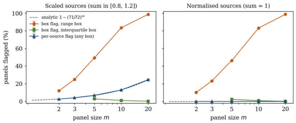
Share of panels flagged for a direct overflow against panel size, for scaled (left) and normalised (right) independent sources, with 95% Wilson intervals (smaller than the markers) and the analytic per-source curve of Proposition 7.
Figure 2.
Share of panels flagged for a direct overflow against panel size, for scaled (left) and normalised (right) independent sources, with 95% Wilson intervals (smaller than the markers) and the analytic per-source curve of Proposition 7.
- 1.
- The range box never misses and increasingly over-flags. Its false-negative share is zero in every cell (Proposition 3). Under the independent scaled model it flags a direct overflow in 12.0% of two-source panels and 98.7% of twenty-source panels, while a source overflows in 2.6% and 24.5% of them, in agreement with % and %. The mechanism is that of Proposition 5: the channel maxima tend to their suprema, whose sum exceeds 1, while the maximum of the per-source sums tends to a supremum only slightly above 1; Proposition 5 gives the limits, not the rates, and the shares grow with in both cases.
- 2.
- For normalised sources every box flag is a false positive. The per-source index is identically zero, so the 83.2% of ten-source panels flagged by the range box measure polarisation, not overflow.
- 3.
- The interquartile box under-flags. Discarding the tails discards the overflowing sources: at it flags 1.1% of panels while 13.0% contain an overflowing source, and it underestimates the magnitude in 12.8% of panels; its signed difference is negative on average.
- 4.
- A common-factor mixture shrinks both flags. With the sources cluster around a common draw; this changes the dependence between sources and the marginal distribution of each source (before scaling and clipping the variance of each coordinate is halved, since ; after scaling and clipping the ratio is about ; the analytic value no longer applies), and the range box flags 21.2% of ten-source panels against 83.6% when independent; the false-positive share falls accordingly. The variant does not isolate the effect of dependence, since marginals and dependence move together; it shows that the shares of Table 3 are properties of the generative model and not of the panel size alone.
- 5.
- The six types are informative for small panels and concentrate on two types for large range boxes. On range boxes of ten or more independent sources the Strong and Mixed types account for essentially all panels, with a residual of other types below one percent at ; the interquartile box, being narrower, spreads over the types. This is an empirical predominance under these models, not a mathematical reduction of the taxonomy.
10. Diagnostics for Panels
10.1. States
Given a panel, its range box and a threshold on the per-source index (a domain quantity, not a constant of the mathematics), exactly one of four states holds, and each is a statement about computed quantities:
- S0: no direct overflow anywhere; by Proposition 3, .
- S1: box excess only; the panel is polarised.
- S2: some source overflows, below the escalation threshold.
- S3: escalate; re-eliciting other sources does not change the overflowing one.
Not exceeding never licenses the conclusion : three identical sources with are in S2, not in S1. The state is reported together with the identified interval of Corollary 1, the type, the necessary flags, and the and intervals, which the overflow indices do not see (Remark 3).
10.2. Influence
For a panel of sources the width influence measures how much source widens the box; it is positive exactly when alone attains an extreme of some channel, and it is not a conflict measure. (For the box of the empty panel is undefined; the implementation adopts the conventions and .) For state S1 the relevant quantity is the direct-index influence , together with the sets of sources attaining and . A source that only stretches has and : in the panel of two copies of , two of and one , the width influences are and single out the fifth source, whereas with or without it; is identically zero because the polar extremes are tied, and the reported diagnosis is that the polarisation is carried by the sets and jointly. A zero leave-one-out influence therefore never implies absence of polarisation; it signals ties or spread. No causal reading is attached to .
10.3. Interval Disagreement
For two intervals the length overlap , with when both are the same point, is the Jaccard index of the segments; it is for a point strictly inside a non-degenerate interval and for two intervals that only touch, so does not mean incompatibility. Incompatibility is measured by the separation , positive exactly when the intervals are disjoint. Two boxes are in strong disagreement when their or their intervals are disjoint; in moderate disagreement when they are not and or for a tolerance ; in agreement otherwise. This classifies numerical reports; it does not diagnose the epistemic origin of a disagreement.
10.4. A Heuristic Revision Procedure
- Compute the state (Section 10.1). Stop in S0, S2 and S3 with the corresponding report.
- In S1, compute and the extreme-attaining sets. If no exceeds a tolerance , stop: the polarisation is distributed or tied.
- Otherwise request clarification from the sources with (a domain step) and replace their reports. If nothing changed, stop at a fixed point; otherwise return to step 1, up to a maximum number of rounds.
The procedure terminates within the maximum number of rounds. It guarantees nothing else: an arbitrary clarification step can oscillate or increase every index, so no convergence to consensus and no monotone decrease of conflict are claimed. The implementation copies the panel before each round, so that the caller’s data are never mutated, and compares reports channel by channel in a fixed order. In the worked example the state is S1 with ; if clarification leads source 3 to revise from to and nothing else changes, the new box has , the state is S0 after one round, and the type is Mixed (, ): the remaining over-allocation is the panel’s combined indeterminacy and neutrality, to be read from the and intervals.
10.5. Instantiation
An instantiation specifies the sources, the elicitation of under Definition 2 with the segmentation rule stated, the construction of intervals and what their widths mean, the joint indices reported alongside the box indices, the thresholds , and the action attached to each state. Panels of annotators [23,24,25], of retrieved passages in retrieval-augmented generation [26] and of laboratories interpreting the same variant [27] are settings in which per-source reports exist and the joint indices can be computed; none has been run in this paper and the thresholds are uncalibrated.
11. Discussion and Limitations
- 1.
- Scope of the identification theorem. Theorem 1 assumes that the box is the exact range box of the panel. For quantile, Student or bootstrap boxes the bounds are not panel extremes and the theorem does not apply; for a single source reporting intervals no per-source index exists and only the possible/necessary readings of Section 4 are available.
- 2.
- The unit threshold is a convention on a cardinal scale and is not invariant under monotone rescaling (Section 3.3). The overflow types do not define contradiction in a logical sense; no consequence relation is given.
- 3.
- Identifiability ofandrests on the protocol and on its segmentation rule; the information-response hypothesis of Remark 1 is untested.
- 4.
- The algebra is auxiliary and its three negations answer different purposes under the evidential reading of and (Section 7); the ranking rule is a convention and admits ties on boxes.
- 5.
- Confidence-interval constructions estimate a mean, not disagreement, and four marginal intervals give no joint coverage without adjustment.
- 6.
- The simulation is synthetic. Its rates are properties of the generative models, anchored by Proposition 7, not estimates of real-world contradiction rates; the common-factor variant shows that the shares change substantially with the generative mechanism, without isolating the effect of between-source dependence.
- 7.
- Thresholds are uncalibrated and no instantiation of Section 10.5 has been run. An earlier draft reported a qualitative negative result from a companion experiment on retrieval-augmented generation; because its data, protocol and results are not part of a verifiable public artefact at the time of writing, that claim is withdrawn from this version and will be reported separately when the artefact is available.
- 8.
- Priority and depth. Theorem 1 combines elementary facts, and a reader may ask for a wider comparison. None of the works reviewed in Section 2, read in full, states an equivalent identification region for neutrosophic quadruples; interval arithmetic gives only the naive lower end; the coordinatewise lower-bound argument has antecedents elsewhere [28]; and the attribution of the characterisation remains open to correction from sources outside that review. What the paper offers is not depth of technique but exactness: the region is sharp, its endpoints and interior are constructed, and the bound is what a practitioner needs to read a box built from a panel.
12. Conclusions
An interval-valued (T, I, N, F) element built channel by channel from a panel retains the range of each channel but not the pairing of channels within a source. This paper has shown what it retains about the panel’s per-source overflows: an upper bound for the range box (Proposition 3), a sharp identified interval for the largest per-source sum over any set of channels (Theorem 1 and Corollary 1), and sufficient numbers of sources for realising each value (Proposition 4). It has separated the type of a box, a statement about its upper corner, from statements about all of its points (Propositions 1 and 2), and it has anchored a reproducible simulation to a closed-form overflow probability (Proposition 7), showing how, for twenty independent sources under the scaled model, a range box flags a direct overflow in 99% of panels while 25% contain an overflowing source, and how a common-factor mixture lowers both shares. The diagnostics of Section 10 turn these results into a state classification that reports what was computed and no more. Taken together, the results say what the four-channel representation retains when it is used with intervals: the box keeps the range of every channel, the per-source indices keep the largest overflow of every channel sum, and the identified interval says how much of the latter the former determines. Neither object recovers the individual reports, their frequencies or their dispersion beyond the ranges. The comparison with normalised representations is one of what the reported channels can express, not of accuracy: with and elicited as free intensities, the pair of box and per-source indices separates source-level direct overflow from overflow introduced by marginal aggregation, a distinction that vanishes when the same channels are constrained to be shares of a unit (Remark 4). For multi-source AI systems, the practical rule is the one the identification result supports: keep the per-source quadruples, report the box together with the per-source indices, and act on the computed state. The natural continuations are empirical: an elicitation study of Definition 2 with a stated segmentation rule, and a calibration of thresholds on panels with per-source reports.
Author Contributions
Conceptualization, F.S. and M.Y.L.-V.; methodology, M.Y.L.-V.; formal analysis, M.Y.L.-V. and F.S.; software, M.Y.L.-V.; validation, M.Y.L.-V.; writing, original draft preparation, M.Y.L.-V.; writing, review and editing, F.S. and M.Y.L.-V. All authors have read and agreed to the published version of the manuscript.
Funding
This research received no external funding.
Data Availability Statement
The reference implementation (ivtinf.py), its test suite, the generated results (numbers.json, tables.md) and the figure scripts accompany the manuscript as Supplementary Materials; every number in the text is produced by them. No real data were used.
Conflicts of Interest
F.S. is a Guest Editor of the Special Issue to which this manuscript is submitted; the manuscript is to be handled by an independent editor in accordance with the journal’s policy. The authors declare no other conflicts of interest.
Use of Generative Artificial Intelligence
Large language models were used under the authors’ direction: Claude (Anthropic), ChatGPT (OpenAI), DeepSeek and Mistral models as adversarial reviewers of earlier drafts, and Claude Code (Anthropic) to assist in drafting and editing text and code. Every mathematical statement in this version was re-derived by the authors, and every numerical value is produced by the accompanying implementation. No content generated by these systems was accepted without verification.
References
- Smarandache, F. (T, I, N, F) Neutrosophic Set and Logic (Truth, Indeterminacy, Neutrality, Falsehood). Critical Review 2017, XIV, 20–28.
- Smarandache, F. Neutrosophy: Neutrosophic Probability, Set, and Logic; American Research Press: Rehoboth, NM, USA, 1998;
- Ahmad, M. Envelope Geometry and Information Refinement of (T,I,N,F) Neutrosophic Quadruples. Neutrosophic Sets and Systems 2026, 100, 369–379.
- Chatterjee, R.; Majumdar, P.; Samanta, S.K. On Some Similarity Measures and Entropy on Quadripartitioned Single Valued Neutrosophic Sets. Journal of Intelligent & Fuzzy Systems 2016, 30, 2475–2485. [CrossRef]
- Pramanik, S. Interval Quadripartitioned Neutrosophic Sets. Neutrosophic Sets and Systems 2022, 51, 146–156.
- Bag, U.; Pramanik, S. Some Properties of the Interval Quadripartitioned Neutrosophic Sets. Boletim da Sociedade Paranaense de Matemática 2026, 44, 1–12. [CrossRef]
- Ahmad, M. TINF-Consensus for Multi-Annotator Learning: Separating Neutral Responses from Polarized Disagreement. Neutrosophic Sets and Systems 2026, 100, 380–400.
- Smarandache, F.; Leyva-Vázquez, M.Y. (T, I, N, F) Neutrosophic Weak and Strong Paraconsistency and the Epistemics of Artificial Intelligence: Uncertainty, Pluralism, and the Decolonial Turn in Alignment. Neutrosophic Sets and Systems 2026, 100, 470–481.
- Atanassov, K.T.; Gargov, G. Interval Valued Intuitionistic Fuzzy Sets. Fuzzy Sets and Systems 1989, 31, 343–349. [CrossRef]
- Atanassov, K.T. Intuitionistic Fuzzy Sets. Fuzzy Sets and Systems 1986, 20, 87–96. [CrossRef]
- Wang, H.; Smarandache, F.; Zhang, Y.-Q.; Sunderraman, R. Interval Neutrosophic Sets and Logic: Theory and Applications in Computing; Hexis: Phoenix, AZ, USA, 2005;
- Rivieccio, U. Neutrosophic Logics: Prospects and Problems. Fuzzy Sets and Systems 2008, 159, 1860–1868. [CrossRef]
- Moore, R.E. Interval Analysis; Prentice-Hall: Englewood Cliffs, NJ, USA, 1966;
- Smarandache, F. Degree of Dependence and Independence of the (Sub)components of Fuzzy Set and Neutrosophic Set. Neutrosophic Sets and Systems 2016, 11, 95–97.
- Dempster, A.P. Upper and Lower Probabilities Induced by a Multivalued Mapping. Annals of Mathematical Statistics 1967, 38, 325–339. [CrossRef]
- Shafer, G. A Mathematical Theory of Evidence; Princeton University Press: Princeton, NJ, USA, 1976;
- Smets, P.; Kennes, R. The Transferable Belief Model. Artificial Intelligence 1994, 66, 191–234. [CrossRef]
- Advances and Applications of DSmT for Information Fusion; Smarandache, F., Dezert, J., Eds.; American Research Press: Rehoboth, NM, USA, 2004; Vol. 1;
- Jøsang, A. Subjective Logic: A Formalism for Reasoning Under Uncertainty; Springer: Cham, 2016;
- Dubois, D.; Prade, H. Possibility Theory: An Approach to Computerized Processing of Uncertainty; Plenum Press: New York, 1988;
- Walley, P. Statistical Reasoning with Imprecise Probabilities; Chapman & Hall: London, 1991;
- Manski, C.F. Partial Identification of Probability Distributions; Springer: New York, 2003;
- Aroyo, L.; Welty, C. Truth Is a Lie: Crowd Truth and the Seven Myths of Human Annotation. AI Magazine 2015, 36, 15–24. [CrossRef]
- Uma, A.N.; Fornaciari, T.; Hovy, D.; Paun, S.; Plank, B.; Poesio, M. Learning from Disagreement: A Survey. Journal of Artificial Intelligence Research 2021, 72, 1385–1470. [CrossRef]
- Dawid, A.P.; Skene, A.M. Maximum Likelihood Estimation of Observer Error-Rates Using the EM Algorithm. Journal of the Royal Statistical Society: Series C (Applied Statistics) 1979, 28, 20–28. [CrossRef]
- Xie, J.; Zhang, K.; Chen, J.; Lou, R.; Su, Y. Adaptive Chameleon or Stubborn Sloth: Revealing the Behavior of Large Language Models in Knowledge Conflicts. In Proceedings of the Twelfth international conference on learning representations (ICLR 2024); 2024.
- Landrum, M.J.; Lee, J.M.; Benson, M.; Brown, G.R.; Chao, C.; Chitipiralla, S.; Gu, B.; Hart, J.; Hoffman, D.; Jang, W.; et al. ClinVar: Improving Access to Variant Interpretations and Supporting Evidence. Nucleic Acids Research 2018, 46, D1062–D1067. [CrossRef]
- Ravi, P.S.; Tunçel, L. Approximation Ratio of LD Algorithm for Multi-Processor Scheduling and the Coffman–Sethi Conjecture 2015.
- Belnap, N.D. A Useful Four-Valued Logic. In Modern uses of multiple-valued logic; Dunn, J.M., Epstein, G., Eds.; Reidel: Dordrecht, 1977; pp. 5–37.
- Dunn, J.M. Intuitive Semantics for First-Degree Entailments and “Coupled Trees.” Philosophical Studies 1976, 29, 149–168.
- Priest, G. The Logic of Paradox. Journal of Philosophical Logic 1979, 8, 219–241.
- Carnielli, W.; Rodrigues, A. An Epistemic Approach to Paraconsistency: A Logic of Evidence and Truth. Synthese 2019, 196, 3789–3813. [CrossRef]
- Klein, D.; Majer, O.; Rafiee Rad, S. Probabilities with Gaps and Gluts. Journal of Philosophical Logic 2021, 50, 1107–1141. [CrossRef]
- Efron, B.; Tibshirani, R.J. An Introduction to the Bootstrap; Chapman & Hall: New York, 1993;
Figure 1.
Projection of the worked example onto the
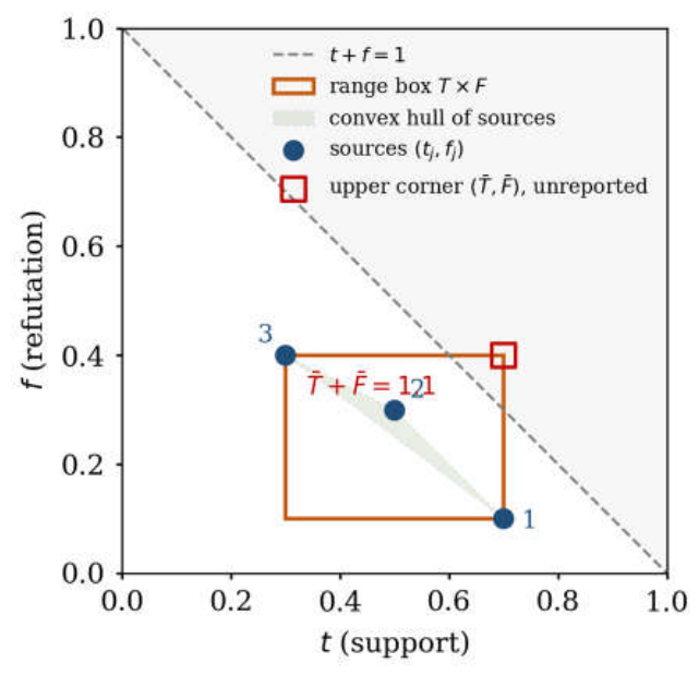
Table 2.
Point reports of three synthetic sources.
| Source | Total | Reliability | |||||
| 1 | 0.7 | 0.1 | 0.1 | 0.1 | 1.0 | 0.8 | 0.9 |
| 2 | 0.5 | 0.2 | 0.1 | 0.3 | 1.1 | 0.8 | 0.6 |
| 3 | 0.3 | 0.3 | 0.2 | 0.4 | 1.2 | 0.7 | 0.3 |
Disclaimer/Publisher’s Note: The statements, opinions and data contained in all publications are solely those of the individual author(s) and contributor(s) and not of MDPI and/or the editor(s). MDPI and/or the editor(s) disclaim responsibility for any injury to people or property resulting from any ideas, methods, instructions or products referred to in the content. |
© 2026 by the authors. Licensee MDPI, Basel, Switzerland. This article is an open access article distributed under the terms and conditions of the Creative Commons Attribution (CC BY) license (http://creativecommons.org/licenses/by/4.0/).
Copyright: This open access article is published under a Creative Commons CC BY 4.0 license, which permit the free download, distribution, and reuse, provided that the author and preprint are cited in any reuse.