

Submitted:
08 September 2026
Posted:
10 September 2026
You are already at the latest version
Abstract
This article examines volatility, tail risk, temporal dependence, scaling behavior and simulation-based uncertainty in daily futures price series for coffee, Brent oil and gold during 2016-2025. The empirical object is defined as a set of provider-reported historical futures series obtained from Investing.com and transformed into logarithmic prices, logarithmic returns, absolute returns, squared returns, annualized 30-day rolling volatility, standardized returns and base-100 indices. In response to the methodological limitations inherent in secondary market-data aggregation, the study does not treat the downloaded series as exchange-certified individual contract histories, nor does it infer unobserved maturity-specific rollover rules. Instead, it positions the data as a transparent financial-risk input and evaluates the consequences of source status, contract identification and calendar irregularity for empirical interpretation. The results show non-Gaussian returns, heavy tails, heterogeneous volatility and stronger dependence in squared returns than in simple returns. Brent oil records the largest tail exposure, the highest kurtosis and the deepest maximum drawdown, while gold exhibits the most visible calendar irregularity. DFA exponents remain close to 0.5, indicating that strong long-memory claims are not supported without additional robustness tests. MF-DFA curves and Monte Carlo fan charts are therefore interpreted as exploratory risk-diagnostic tools rather than confirmatory evidence of multifractality or calibrated forecasts. The article contributes to risk and financial management by offering a cautious, reproducible and empirically delimited framework for comparing commodity futures relevant to Colombia.
Keywords:
commodity futures
; financial risk
; volatility
; tail risk
; Brent oil
; coffee futures
; gold futures
; logarithmic returns
; DFA
; MF-DFA
; Monte Carlo simulation
; Colombia
1. Introduction
Commodity futures are central instruments for financial-risk analysis because their prices synthesize expectations about supply, demand, inventories, geopolitical tensions, monetary conditions and uncertainty. In agricultural, energy and precious-metal markets, futures prices are not merely observed levels; they are signals that condense expectations about future scarcity, risk premia, hedging demand and speculative positioning. The early formalization of speculative pricing by Bachelier (1900), the efficient-market debate developed by Fama (1970), Mandelbrot’s evidence on irregular speculative price variation (Mandelbrot 1963), and the stylized facts summarized by Cont (2001) jointly establish that commodity futures require analytical treatment beyond simple level inspection. Their empirical behavior is better understood through return distributions, volatility dynamics, tail behavior and temporal dependence.
Coffee, Brent oil and gold were selected because they represent three differentiated channels of exposure for a small open economy such as Colombia. Coffee is linked to agricultural exports, rural income transmission and commodity-price exposure in productive regions. Brent oil operates as a global energy benchmark and is connected with external revenues, fiscal expectations, exchange-rate pressures and geopolitical shocks. Gold, in turn, is widely analyzed as a hedging and safe-haven asset during periods of market stress (Baur and Lucey 2010). Studying these three series under a common framework provides a comparative setting in which heterogeneous markets can be examined without forcing them into identical economic interpretations.
The analytical problem addressed in this article is not limited to documenting that commodity prices fluctuate. The central issue is whether daily futures price series, once transformed into financial variables, reveal sufficiently informative patterns for risk measurement, volatility monitoring, dependence diagnostics and scenario analysis. This perspective is consistent with the financial econometrics tradition in which nominal prices are transformed into returns, squared returns, standardized returns and volatility measures before inference is attempted (Box et al. 2015; Campbell et al. 1997). Such transformations are essential because commodity futures differ in quotation units, price levels, market calendars and shock transmission mechanisms.
Conditional heteroscedasticity and volatility clustering have long been recognized as core features of financial series. ARCH and GARCH models formalize the idea that the conditional variance evolves over time and that large shocks tend to be followed by periods of elevated volatility (Engle 1982; Bollerslev 1986). These models remain relevant for commodity markets because energy, agricultural and metal futures are frequently exposed to abrupt supply disruptions, geopolitical events, monetary-policy changes and financial flight-to-quality episodes. Even when the present study does not estimate a full GARCH specification as the main empirical model, the construction of squared returns, absolute returns and rolling volatility provides the necessary diagnostic foundation for such extensions.
The article also evaluates scaling diagnostics with caution. Fractal geometry and fractal market analysis provide conceptual language for examining irregularity, scale dependence and heterogeneous investment horizons (Mandelbrot 1982; Peters 1994). Long-memory methods, including fractional integration and persistence diagnostics, have been used to examine whether shocks decay slowly over time (Hurst 1951; Granger and Joyeux 1980). Nevertheless, the literature also warns that apparent persistence can arise from structural breaks, heteroscedasticity, short-memory effects or heavy tails rather than from genuine long-range dependence (Hosking 1981; Baillie 1996). This warning is directly relevant here because the estimated DFA exponents remain near 0.5.
The use of R/S analysis, detrended fluctuation analysis and multifractal detrended fluctuation analysis therefore has an exploratory function in this study. Beran (1994), Lo (1991), Teverovsky et al. (1999) and Peng et al. (1994) show that persistence diagnostics must be interpreted carefully, while Kantelhardt et al. (2002) extend fluctuation analysis toward multifractal structures. Econophysics has contributed additional tools for identifying scaling behavior and complex dependence in financial systems (Mantegna and Stanley 1995; Mantegna and Stanley 2000). However, this article does not present DFA or MF-DFA as proof of strong memory or confirmed multifractality; it uses them to delimit what the data can and cannot support.
A second methodological issue concerns data provenance. The manuscript originally submitted to Data emphasized the processed dataset as the primary contribution. The review process made clear that a stronger financial-risk framing is required. Investing.com is a secondary aggregator rather than the exchange of record. Consequently, the downloaded series must be treated as provider-reported historical futures series. This distinction matters because exchange, maturity, rollover rule and active-contract definition can affect futures-return measurement. The revised article explicitly defines the empirical object, reports the limitations of contract metadata, and avoids claiming that the series identify maturity-specific contract histories or official continuous futures constructed directly from exchange settlement files (Investing.com 2026).
Data transparency and reproducibility remain important, but they are no longer presented as the sole contribution. The FAIR principles emphasize findability, accessibility, interoperability and reusability (Wilkinson et al. 2016). Research on data infrastructure and sharing practices shows that empirical value depends on organization, preservation, documentation and auditability (Borgman 2015; Tenopir et al. 2011). In computational finance, reproducibility requires clear inputs, explicit transformations and verifiable analytical decisions (Peng 2011; Stodden et al. 2018). The tidy-data framework also supports the identification of observational units, variables and values in a form that can be imported into statistical software (Wickham 2014).
The revised contribution is therefore located at the intersection of commodity-risk analysis, financial econometrics and reproducible empirical design. The article transforms daily closing futures prices into a set of risk-relevant variables; documents the source status and contract-series limitations; identifies calendar irregularities, especially in gold; evaluates distributional and dependence properties; and interprets scaling and Monte Carlo outputs as exploratory diagnostics rather than definitive forecasts. This orientation corresponds more closely to the scope of a financial-risk journal than to a pure data-journal submission.
The article is organized as follows. Section 2 describes the data source, contract-series definition, preprocessing steps, quality-control strategy, risk diagnostics, scaling tools and Monte Carlo design. Section 3 presents the empirical evidence on market coverage, calendar irregularity, return distribution, volatility, temporal dependence, scaling and scenario analysis. Section 4 discusses the implications for commodity-risk analysis and identifies the limitations that condition interpretation. Section 5 concludes and indicates routes for future research.
2. Materials and Methods
The methodological design follows a sequential logic. First, the empirical object is defined as a set of provider-reported daily futures series rather than as exchange-certified individual contract histories. Second, the prices are transformed into returns and volatility-related variables that permit comparable risk analysis across heterogeneous commodities. Third, calendar coverage and source limitations are evaluated before interpreting volatility, dependence or scaling. Fourth, descriptive, tail-risk, dependence and Monte Carlo diagnostics are implemented under an explicitly cautious interpretation.
2.1. Data Source, Market Scope and Continuous-Series Definition
The database was constructed from daily closing futures prices for coffee, Brent oil and gold for the period 2016-2025. The source is Investing.com, a public financial-data platform that aggregates historical price information from different market instruments. For this reason, the empirical object is defined as a provider-reported continuous historical futures series. The study does not infer unobserved maturity, delivery month, exchange-level rollover date or active-contract selection rule beyond the information visible in the downloaded files. This delimitation addresses an essential point for futures research: returns estimated from a vendor-reported continuous series should not be interpreted as returns from a single maturity-specific contract.
Table 1 reports the market segment, provider label, contract family, quotation unit, source and empirical treatment of each series. The table is used to separate the observable information contained in the downloaded files from the exchange-level contract metadata that are not directly verifiable in the dataset. This distinction prevents artificial certainty about contract maturity or rollover rules and establishes a more defensible empirical basis for risk analysis.
Table 1 makes explicit that the analysis uses historical price series as reported by the provider. The contract family is identified to contextualize the market instrument, but the article does not reconstruct a proprietary continuous-futures rule. This clarification limits the inferential scope of the study and prevents the empirical results from being interpreted as official exchange settlement, maturity-specific contract performance or contract-arbitrage evidence.
The distinction between a provider-reported series and an exchange-reconstructed continuous futures series is central for the reader. The article therefore refrains from treating the contract identifier as a complete contractual field. It is a market label that permits the construction of a commodity-specific return series, while the absence of delivery-month metadata restricts inference about rollover premia, term-structure behavior and maturity effects. This limitation is incorporated into the design rather than concealed in the results.
2.2. Data Preprocessing and Variable Construction
The preprocessing stage converts heterogeneous commodity prices into comparable financial variables. Because coffee, Brent oil and gold are quoted in different units, direct level comparisons are analytically limited. The transformation pipeline therefore stabilizes scale through logarithmic prices, measures relative variation through logarithmic returns, captures fluctuation magnitude through absolute and squared returns, approximates recent risk through 30-day annualized rolling volatility, normalizes cumulative trajectories through base-100 indices and identifies relative extremes through standardized returns. These transformations are standard in financial econometrics, but their role in this article is to provide a transparent and auditable basis for risk diagnostics rather than to claim methodological novelty in the algebra itself.
The closing price in logarithmic scale, aligned with Equation (1), is the first transformation performed. This operation preserves the temporal order of prices and facilitates the subsequent construction of continuous returns.
where represents the logarithmic price of commodity on day ; is the closing price observed for commodity i on day ; and denotes the natural logarithm operator. This variable makes it possible to work on a scale compatible with continuous returns and facilitates the comparison of series with different quotation units.
The daily logarithmic return is obtained as the continuous variation between two consecutive prices of the same commodity, according to Equation (2). The operation is executed within each asset and while respecting its own trading calendar.
where is the daily logarithmic return of commodity on day ; is the current closing price; and is the immediately preceding closing price within the same commodity. The subscript identifies the asset and the subscript identifies the trading day. This definition avoids calculating returns between different assets or unordered dates.
The absolute magnitude of movements is obtained through Equation (3). This variable removes the direction of change and preserves the intensity of the variation, making it useful for examining episodes of high market mobility.
where represents the absolute value of the logarithmic return of commodity on day ; is the daily logarithmic return; and corresponds to the absolute-value operator. This variable is useful for studying variation intensity, stress episodes and persistence in return magnitude.
The squared return, defined in Equation (4), amplifies larger variations and provides an elementary approximation to second-moment dynamics. Its inclusion makes it possible to contrast dependence in simple returns with persistence in variability.
where corresponds to the square of the logarithmic return of commodity i on day t; and represents the return raised to the square. This variable is a frequent input for diagnosing volatility dependence and risk clustering.
The 30-day annualized rolling volatility is calculated by applying Equation (5). This measure analyzes return variability and identifies stress periods without using parametric conditional models.
where represents the 30-day annualized rolling volatility of commodity on day ; 252 is the annualization factor for daily returns; is the return observed days earlier within the same commodity; is the mean return in the 30-observation rolling window; and k=0,...,29 indicates that the current return and the previous 29 valid returns are used. The measure is calculated independently for each asset.
To compare accumulated trajectories across assets with different quotation units, the base-100 index formalized in Equation (6) is used. The transformation preserves the relative dynamics of each market without artificially equating their nominal levels.
where is the normalized index of commodity on day ; is the closing price on date t; and corresponds to the first valid price in the commodity i series. This transformation does not replace return analysis, but it makes it possible to observe relative trends on a common scale.
The standardized return is defined in Equation (7). This variable center and scales the returns of each commodity with respect to its own distribution, enabling the identification of relative extreme events within each market.
where represents the standardized return of commodity on day ; is the daily logarithmic return; is the sample mean of returns for commodity ; and is the sample standard deviation of the returns of the same asset.
2.3. Data-Quality and Calendar-Irregularity Assessment
Data-quality assessment is organized around both computational integrity and financial interpretation. The arithmetic consistency between prices and returns is necessary but not sufficient. A financially meaningful validation must also examine whether the calendar structure is regular, whether the series contains missing weekdays, whether the source permits contract-level identification and whether the available metadata support the intended interpretation. The quality-control strategy therefore distinguishes internal calculation checks from empirical limitations that cannot be resolved without primary exchange data.
Table 2 summarizes the validation criteria used in the study. These criteria do not claim to certify the series as official exchange data; they document the conditions under which the processed variables can be interpreted. The distinction is important because correctly calculated returns do not, by themselves, validate rollover rules, maturity structure or provider coverage.
Table 2 indicates that the processed variables are arithmetically consistent and traceable to their source, but it also establishes the boundaries of interpretation. The presence of a valid price-return relationship confirms the computational pipeline, while calendar diagnostics and source-status disclosure define the limits of financial inference. The article therefore treats data quality as a combination of reproducible calculation, transparent limitation and cautious empirical use.
The calendar assessment is especially important for gold. The observed reduction in the number of records in several years can affect diagnostics that depend on temporal regularity. For that reason, the study does not impose interpolation, does not fill missing days with artificial prices and does not force the three commodities into a balanced panel. The analysis retains commodity-specific sequences and interprets comparisons as descriptive rather than as strict synchronized-panel inference.
2.4. Descriptive, Tail-Risk and Dependence Diagnostics
The empirical diagnostics are selected to characterize risk, not to force a single structural model. Descriptive statistics summarize location and dispersion; empirical quantiles and expected shortfall describe downside tails; maximum drawdown captures cumulative loss episodes; Jarque-Bera tests assess deviations from Gaussian behavior; autocorrelation and Ljung-Box statistics evaluate dependence in returns and squared returns. Together, these tools provide a risk-oriented profile of each commodity while preserving the distinction between descriptive evidence and validated forecasting performance.
The Jarque-Bera test makes it possible to assess whether the deviation of returns follows a normal distribution. The articulation of skewness and kurtosis in Equation (8) synthesizes the distance between the empirical distribution and Gaussian behavior.
where is the Jarque-Bera statistic for commodity ; is the number of valid returns; represents sample skewness; and corresponds to Pearson kurtosis. High values of JBi are consistent with non-Gaussian distributions, a common situation in financial series with heavy tails.
The order autocorrelation in Equation (9) makes it possible to observe linear dependence in returns and second-moment dependence when applied to squared returns. This differentiates mean dynamics from variability persistence.
where is the autocorrelation of commodity at lag ; is the current return; and is the return observed periods earlier. This measure allows linear dependence to be assessed at different lags.
The Ljung-Box statistic in Equation (10) jointly evaluates the significance of autocorrelations up to lag m and summarizes temporal dependence without relying on a single isolated lag.
where represents the Ljung-Box statistic of commodity up to lag ; is the number of valid observations; is the autocorrelation of order ; and is the total number of lags evaluated. The statistic summarizes the joint significance of autocorrelations.
2.5. Scaling Diagnostics and Monte Carlo Scenario Design
Scaling diagnostics and simulation are implemented as exploratory extensions of the risk analysis. The Hurst coefficient, DFA and MF-DFA are used to examine whether the transformed series display scale-dependent patterns. Their interpretation is deliberately cautious because exponents close to 0.5 do not establish strong long memory and because calendar irregularity can affect fluctuation functions. The Monte Carlo exercise uses empirical bootstrap draws from historical logarithmic returns, 10,000 simulated paths per commodity, a 60-trading-day horizon and a fixed random seed of 12345. The simulated fan charts report median trajectories and P5-P95 intervals; they are scenario bands, not calibrated VaR or Expected Shortfall forecasts.
The R/S fraction of the Hurst coefficient is used as an initial approximation for observing temporal persistence through Equation (11). The value of this coefficient allows a preliminary analysis of scaled behavior and is interpreted together with more robust diagnostics.
where represents the cumulative range of deviations from the mean in a window of size ; s the standard deviation within that window; is a proportionality constant; and is the Hurst exponent. Values close to 0.5 are compatible with the absence of strong linear persistence.
Equation (12) presents the accumulation of data from DFA, whose transformation converts centered returns into an accumulated trajectory on which scale fluctuations are evaluated.
where represents the cumulative profile of commodity i up to temporal position ; is the logarithmic return observed at ; and is the mean return of the series. This transformation makes it possible to evaluate fluctuations around local trends.
The slope of the DFA fluctuation function defined in Equation (13), on a log-log scale, approximates scaling behavior and makes it possible to evaluate whether the series is persistent, antipersistent or close to randomness.
where represents the DFA fluctuation function of commodity for scale ; is the number of observations evaluated; is the cumulative profile; and represents the local trend estimated within each window of size s.
The generalized MF-DFA function, summarized in Equation (14), extends the analysis to different q orders, thereby making it possible to differentiate small and large fluctuations, which is relevant for markets exposed to ordinary and extreme episodes.
where represents the generalized fluctuation function of commodity for order and scale ; is the number of segments; is the local detrended variance of segment at scale . Positive values of emphasize large fluctuations and negative values emphasize small fluctuations.
The Monte Carlo simulation described in Equation (15) translates the historical return distribution of each commodity into possible short-horizon price paths. The exercise is based on empirical bootstrap resampling of historical daily logarithmic returns and therefore preserves the unconditional distributional features of each series but does not model conditional volatility dynamics. This design is transparent and replicable, but it must be interpreted as scenario generation rather than as a forecasting system.
The choice of empirical bootstrap is intentionally transparent. It avoids imposing normality on the return distribution and preserves the observed tail behavior of each series. At the same time, it does not capture volatility clustering dynamically, because returns are sampled independently from the historical distribution. This trade-off is declared explicitly so that the simulated fan charts are read as a communication device for uncertainty rather than as a definitive forecasting model.
where is the simulated price of commodity at horizon for trajectory ; is the last observed price; is the simulated return at step of trajectory ; and is the exponential function. The equation makes it possible to construct probabilistic trajectories from simulated returns.
2.6. Computational Environment, Reproducibility and Data Availability
The computational environment is treated as an operational component of the empirical design. The transformation workflow orders observations chronologically, validates positive prices, calculates returns within each commodity, constructs volatility and risk variables, generates figures and produces diagnostic tables. Reproducibility is supported through the Supplementary Files, which contain the processed dataset, variable dictionary, processing notes and quality-control files. Because the original price series were obtained from a secondary aggregator, users should consult the licensing and redistribution conditions of the original provider before reusing raw market data.
Table 3 summarizes the processed variables and their analytical role. The table is retained because it connects each derived field with a concrete risk, volatility or scaling function. It is not presented as a repository checklist; it is the bridge between the raw price series and the empirical diagnostics developed in the results section.
The variables presented in Table 3 define the analytical vocabulary of the article. Closing prices provide market levels; logarithmic returns provide relative variation; absolute and squared returns capture fluctuation magnitude and second-moment behavior; rolling volatility captures recent risk; base-100 indices permit cumulative comparison; and standardized returns help identify relative extremes. This structure supports risk analysis without claiming that the transformations alone constitute a novel dataset product.
3. Results
The results are organized around five dimensions: contract and calendar constraints, distributional risk, volatility and temporal dependence, scaling diagnostics, and Monte Carlo scenario analysis. This structure aligns the manuscript with financial-risk management because each empirical result is interpreted according to its contribution to risk measurement, model selection or scenario evaluation. The analysis deliberately separates observed evidence from the limits imposed by source status and calendar irregularity.
3.1. Market Coverage and Calendar Irregularity
The first empirical result concerns the relationship between market coverage and calendar structure. A one-observation difference between valid prices and valid returns is expected because the first price in each series has no preceding observation from which to calculate a return. This confirms the internal calculation of returns, but it does not fully characterize data integrity. Calendar density must also be examined, particularly because gold has fewer observations than coffee and Brent oil.
Table 4 summarizes the coverage profile of the three series and identifies the principal calendar irregularity observed in the data. The purpose is to prevent the analysis from treating all commodities as equally spaced with identical observation density. Calendar irregularity is especially relevant for rolling volatility, autocorrelation, DFA and MF-DFA because those procedures can be affected by gaps or by non-uniform trading records.
Table 4 shows that coffee and Brent oil present relatively stable coverage across the sample, whereas gold contains a more pronounced irregularity. The reduced number of observations in gold is concentrated in several years, especially 2017-2019 and 2022-2025. This does not invalidate the use of gold returns, but it requires cautious interpretation of any cross-commodity comparison and any scaling diagnostic that assumes homogeneous temporal density.
The interpretation of returns and volatility begins with the price-level trajectories displayed in Figure 1. The figure separates coffee, Brent oil and gold into independent panels so that each commodity can be read in its own quotation scale. This avoids misleading visual inference that could arise from comparing US cents per pound, dollars per barrel and dollars per troy ounce on a common nominal axis.
Coffee displays phases of decline, recovery and strong recent increases. Brent oil contains abrupt shock-and-reversal episodes associated with energy-market conditions, while gold shows a persistent upward movement over the later part of the sample. These heterogeneous trajectories reinforce the need to analyze returns and risk measures rather than draw conclusions from nominal price levels alone.
Figure 2 complements the price-level reading through base-100 indices. The normalization sets the first valid observation of each series equal to 100 and permits relative cumulative comparison across commodities with different quotation units. This figure is descriptive rather than inferential; it shows how accumulated price trajectories diverge over the sample.
Figure 2 indicates that coffee and gold experience pronounced cumulative increases toward the end of the period, whereas Brent oil follows a more cyclical path with strong reversals. These differences are consistent with the economic roles of the three commodities and motivate the subsequent analysis of tail risk, volatility and scenario uncertainty.
3.2. Distributional Properties, Tail Risk and Drawdown
The distributional properties of logarithmic returns provide the first risk-management reading of the transformed series. The analysis focuses on mean, standard deviation, empirical downside quantiles, expected shortfall, maximum drawdown, skewness, kurtosis, Jarque-Bera statistics and dependence in squared returns. These indicators jointly describe the magnitude, asymmetry and tail exposure of each market.
Table 5 reports the main distributional and historical-risk diagnostics. VaR and Expected Shortfall are computed from the empirical return distribution and are therefore interpreted as unconditional historical tail measures. They are not presented as regulatory risk forecasts because no dynamic volatility model or backtesting procedure is estimated in this stage.
Table 5 confirms that the three commodities have non-Gaussian return distributions. Brent oil records the highest standard deviation, the most negative 1% historical VaR, the deepest Expected Shortfall and the largest maximum drawdown, which identifies it as the most exposed series in the historical sample. Gold has lower dispersion and drawdown, but its calendar irregularity qualifies any direct comparison. Coffee occupies an intermediate position, with substantial volatility and downside exposure but less extreme tail behavior than Brent oil.
The empirical density of logarithmic returns is shown in Figure 3. The purpose of the figure is to visualize whether the return distribution is concentrated around zero while still preserving tails and extreme observations. This graphical evidence complements the numerical diagnostics reported in Table 5.
Figure 3 shows a central concentration of returns around zero and non-negligible tail observations in all three commodities. The distributional shape supports the use of risk measures that go beyond mean and standard deviation. It also confirms that any modelling strategy based on normality alone would be insufficient for these markets.
3.3. Volatility and Temporal-Dependence Patterns
Volatility and temporal-dependence diagnostics provide a second layer of risk interpretation. The analysis distinguishes between dependence in the conditional mean and persistence in the second moment. This distinction is relevant because commodity markets may show limited autocorrelation in returns while still exhibiting strong volatility clustering through squared or absolute returns.
Continuing with the annualized analysis over 30-day intervals for each commodity, Figure 4 presents rolling volatility, making it possible to identify periods of instability and assess whether the database contains observable risk-concentration episodes before applying conditional models.
Figure 4 shows that volatility is time varying and market specific. Brent oil presents strong volatility bursts, coffee displays persistent episodes of elevated variability, and gold shows narrower but still visible volatility clusters. These patterns justify the inclusion of rolling volatility, absolute returns and squared returns as central variables for financial-risk monitoring.
Figure 5 compares the autocorrelations of returns and squared returns. Together, they make it possible to establish whether dependence is expressed mainly in the mean or in variability, a fundamental distinction for guiding the subsequent use of ARCH/GARCH models or fractional extensions.
Figure 5 indicates that dependence is more visible in squared returns than in simple returns. This pattern is consistent with volatility clustering and suggests that conditional-variance models can be more relevant than mean-equation models for subsequent work. The result should be read as a model-selection indication, not as proof that a specific ARCH/GARCH structure has already been validated.
3.4. Scaling Diagnostics: Cautious Interpretation of Long Memory and Multifractality
Scaling diagnostics are interpreted with explicit caution. The objective is not to claim that the three commodities exhibit strong long memory or confirmed multifractality. Instead, the purpose is to evaluate whether the processed returns generate regular fluctuation curves and whether those curves justify more specialized tests in future research. This distinction responds directly to the risk of overstating persistence when exponents are close to 0.5.
The DFA curves on a log-log scale, shown in Figure 6, display the relationship between temporal scale and fluctuation function, allowing determination of whether the processed returns generate sufficiently regular scaling structures for long-range dependence analysis.
The DFA exponents are close to 0.5, indicating that the evidence does not support a strong long-memory claim. The curves in Figure 6 show usable scaling structure, but the values require cautious interpretation. In particular, any future claim about long memory should incorporate confidence intervals, shuffled or surrogate series, structural-break controls and robustness checks across subperiods.
The visualization of generalized MF-DFA functions with different q orders, as presented in Figure 7, makes it possible to distinguish small and large fluctuations and thereby evaluate whether heterogeneity-of-scaling analysis can be applied to the dataset.
Figure 7 shows separation across q-orders in the generalized fluctuation functions. This pattern is compatible with heterogeneous scaling, but it is not sufficient on its own to establish multifractality. A complete multifractal analysis would require the singularity spectrum, uncertainty estimation, surrogate testing and careful treatment of calendar irregularity. The figure is therefore retained as exploratory evidence of analytical potential rather than as definitive proof.
3.5. Monte Carlo Scenario Analysis
The Monte Carlo exercise is designed as a transparent scenario analysis rather than as a calibrated forecasting model. For each commodity, the simulation draws daily logarithmic returns with replacement from the empirical distribution, generates 10,000 price paths over a 60-trading-day horizon, uses the last observed price as the starting value and fixes the random seed at 12345. This structure makes the fan charts reproducible while avoiding unsupported claims about conditional dynamics.
Figure 8 presents the median trajectory and the P5-P95 interval for each commodity. The width of the fan reflects the historical dispersion of the bootstrapped returns. The bands are not interpreted as VaR or Expected Shortfall because they are not derived from a calibrated risk model with backtesting. They are short-horizon uncertainty scenarios conditioned on the empirical return distribution.
Figure 8 reveals differentiated uncertainty bands across the three commodities. Brent oil displays a wider scenario space consistent with its higher historical volatility and tail exposure. Coffee presents relevant uncertainty over the horizon, while gold shows narrower scenario bands but remains conditioned by its calendar limitations. These findings are useful for stress-testing narratives and risk communication, but not for deterministic forecasting.
3.6. Financial-Risk Management Implications
The empirical evidence can be translated into financial-risk management implications. The return distributions inform tail-risk monitoring; rolling volatility identifies periods of recent market stress; squared-return dependence indicates potential conditional-variance persistence; scaling diagnostics delimit the scope of memory claims; and Monte Carlo fan charts provide a scenario-based representation of uncertainty. These implications are summarized in Table 6.
Table 6 connects each empirical dimension with its risk-management interpretation and with the caution required for responsible use. This structure is designed to avoid overstating the contribution of the dataset while preserving the value of the analysis for financial decision-making, teaching and further modelling.
Table 6 shows that the article contributes not by proposing a new pricing theory, but by offering an integrated empirical reading of volatility, tail risk, temporal dependence and exploratory scaling in three strategic commodity futures markets. The results provide a defensible basis for future work with conditional volatility models, rolling-window tests, cross-market dependence and stress-scenario analysis.
4. Discussion
The findings reposition the manuscript as an empirical contribution to risk and financial management rather than as a pure data article. This distinction is fundamental. The value of the study lies in the integrated diagnosis of commodity-futures risk, the transparent handling of data limitations and the cautious interpretation of scaling and simulation results. The revised framing acknowledges that preprocessing alone does not create a scientifically novel data product; its relevance emerges when the processed variables are used to interpret risk exposure, volatility clustering, tail behavior and scenario uncertainty.
This repositioning is also consistent with the editorial transfer suggested after the Data decision. A journal focused on risk and financial management is a more natural outlet for the article because the strongest contribution is not the originality of the data transformation alone, but the disciplined interpretation of the risk evidence generated from the processed series. The manuscript therefore emphasizes tail exposure, drawdown, volatility clustering, model-selection implications and scenario uncertainty.
The first discussion point concerns data provenance. Using Investing.com introduces a limitation because the platform is a secondary aggregator rather than a primary exchange. This limitation does not make the analysis unusable, but it changes the scope of inference. The results should be interpreted as evidence derived from provider-reported historical futures series, not as official exchange-settlement evidence for maturity-specific contracts. This clarification directly affects the interpretation of returns, rollover effects and contract continuity. Future versions of the research can be strengthened by reconstructing front-month or volume-based continuous futures directly from exchange sources.
The second point concerns calendar irregularity. Gold has fewer observations than coffee and Brent oil, and this difference is not a minor formatting issue. It affects the way volatility, autocorrelation and scaling diagnostics should be read. Preserving each commodity calendar avoids artificial interpolation, but it also means that cross-market comparisons are not based on identical observation density. The article therefore favors univariate diagnostics and descriptive comparison over strong multivariate inference. For future research, an additional sample based only on common trading dates should be estimated and compared with the commodity-specific-calendar results.
The third point concerns the interpretation of tail risk. The empirical values reported for VaR and Expected Shortfall summarize historical downside exposure but do not constitute regulatory forecasts. Brent oil exhibits the most severe downside profile, which is consistent with energy markets’ exposure to geopolitical shocks, demand collapses and supply disruptions. Coffee and gold display different risk profiles: coffee combines agricultural-market volatility with strong recent price movements, while gold exhibits lower dispersion but remains affected by its observational structure. This evidence is relevant for investors, analysts and instructors who need comparative commodity-risk examples.
The fourth point concerns temporal dependence. The evidence that squared returns display stronger dependence than simple returns is consistent with the volatility-clustering literature initiated by Engle (1982) and Bollerslev (1986). Nevertheless, the manuscript avoids estimating a full volatility model without first clarifying data structure and source limitations. This decision is methodologically conservative. The present results indicate that conditional-variance models are appropriate candidates for future work, but the article does not claim that a specific GARCH, EGARCH, TGARCH or FIGARCH model has been selected, estimated and validated.
The fifth point concerns scaling. The DFA exponents close to 0.5 restrict the strength of any long-memory statement. This is consistent with the warnings of Lo (1991), Teverovsky et al. (1999) and Baillie (1996), who show that persistence can be difficult to distinguish from short-memory dependence, structural instability or heteroscedasticity. The revised manuscript therefore moves away from the language of confirmation and adopts the language of diagnostic suitability. MF-DFA outputs are treated in the same way: they indicate that additional multifractal work is possible, not that multifractality has been conclusively demonstrated.
The sixth point concerns Monte Carlo simulation. The fan charts provide a useful visualization of uncertainty because they transform empirical return distributions into short-horizon price-path ensembles. However, a bootstrap simulation without a conditional-volatility equation is not a complete risk-forecasting system. The study therefore separates P5-P95 scenario bands from VaR and Expected Shortfall. Monte Carlo methods are valuable in financial engineering and risk management (Metropolis and Ulam 1949; Glasserman 2004), but their results depend on the return-generating mechanism and on the assumptions imposed on volatility, dependence and sampling.
This risk-oriented interpretation also allows the manuscript to connect with broader financial-management applications. Historical tail measures can support risk dashboards; rolling volatility can identify stress periods; autocorrelation diagnostics can inform model selection; scaling analysis can guide future persistence tests; and scenario fans can support communication of uncertainty. These applications are compatible with the decision-oriented nature of risk management, while remaining transparent about the limits of the underlying data.
The article also opens future methodological extensions. Predictive comparisons could incorporate Diebold and Mariano’s (1995) testing framework once competing forecasting models are estimated. Energy-market scaling can be extended using approaches similar to Alvarez-Ramirez et al. (2008). Cross-market dependence can be explored with wavelet coherence or related time-frequency techniques, as shown in applications by Kristoufek (2015) and Goodell and Goutte (2021). Data-driven probabilistic frameworks such as that of Rodriguez-Sanchez et al. (2026) illustrate how quantitative inputs can be transformed into decision-support platforms under uncertainty.
In the Colombian context, the three commodities have different transmission channels. Coffee is connected with agricultural export income; Brent oil is linked with energy-sector expectations, fiscal sensitivity and exchange-rate pressure; and gold functions as a hedge or safe-haven reference. The article does not estimate a Colombian macroeconomic transmission model, but it supplies risk diagnostics that can be integrated into such models. The limitation is explicit: causal inference requires additional macrofinancial variables, domestic price series, exchange-rate measures and policy indicators.
The main implication is that the manuscript is stronger when it is framed as a cautious empirical study of commodity-futures risk than when it is framed as a standalone data product. The reviewer concerns are therefore incorporated into the article’s architecture: contract metadata are delimited, gold calendar irregularity is documented, long-memory claims are moderated, MF-DFA is treated as exploratory, Monte Carlo assumptions are specified and VaR/Expected Shortfall are separated from scenario bands.
The reliability of the analysis depends on transparency rather than on overstatement. The Supplementary Materials allow the processed variables to be reviewed, while the text states the limits imposed by secondary data, missing observations and non-estimated conditional models. This structure aligns with reproducibility principles (Wilkinson et al. 2016; Peng 2011) while placing the empirical contribution within the risk-management domain rather than within a data-repository logic.
Several limitations remain. The study uses daily data and therefore does not analyze intraday liquidity, bid-ask spreads or high-frequency volatility. It excludes trading volume, open interest, storage costs, convenience yields, domestic Colombian commodity prices and macroeconomic controls. It also does not reconstruct exchange-certified continuous contracts. These restrictions define the scope of the evidence and should guide future extensions rather than being treated as incidental details.
In summary, the revised manuscript provides a risk-based reading of coffee, Brent oil and gold futures for Colombia-relevant commodity exposure. It documents source constraints, transforms prices into risk variables, identifies tail and volatility patterns, interprets scaling cautiously and uses Monte Carlo simulation as a transparent scenario tool. The contribution is therefore empirical, methodological and pedagogical: it demonstrates how processed daily futures data can be converted into a coherent risk-analysis framework without overstating the power of the available information.
5. Conclusions
This article examined volatility, tail risk, temporal dependence, exploratory scaling and Monte Carlo uncertainty in daily futures price series for coffee, Brent oil and gold during 2016-2025. The study was reoriented from a pure data-product argument toward a financial-risk management contribution. This change is important because the evidence is more defensible when the processed variables are used to interpret risk properties than when the manuscript claims that the dataset alone constitutes a novel scientific resource.
The results show that the three commodities preserve non-Gaussian return behavior, heavy tails, time-varying volatility and stronger dependence in squared returns than in simple returns. Brent oil displays the most severe tail-risk and drawdown profile, coffee exhibits substantial volatility associated with agricultural-market dynamics, and gold combines lower dispersion with the most visible calendar irregularity. These findings support the use of commodity-specific risk diagnostics rather than a single homogeneous treatment of all futures series.
The article also demonstrates the need for caution in interpreting long memory and multifractality. DFA exponents close to 0.5 do not establish strong long-range dependence, and MF-DFA curves without singularity spectra, confidence intervals or surrogate tests should not be read as conclusive proof of multifractality. The revised interpretation treats these tools as diagnostic and exploratory, thereby reducing the risk of unsupported methodological claims.
The Monte Carlo exercise contributes a transparent scenario representation based on empirical bootstrap draws from historical logarithmic returns. The P5-P95 fan charts provide uncertainty bands that help compare short-horizon risk across commodities, but they are not equivalent to backtested VaR or Expected Shortfall forecasts. This distinction clarifies the risk-management meaning of the simulation and prevents an overextension of the results.
Future research should strengthen the empirical design by reconstructing continuous futures series directly from exchange data, documenting exact rollover rules, estimating robustness under common-date samples, incorporating volume and open interest, applying conditional-volatility models, implementing formal multifractal spectra and comparing forecasting models with out-of-sample accuracy tests. These extensions would allow the present framework to evolve into a more complete commodity-risk platform for Colombia and other open economies.
Supplementary Materials
The processed dataset, variable dictionary, processing notes, quality-control files and reproduction scripts are available as supplementary material to the article. The supplementary files support the transformation from closing prices to logarithmic returns, squared returns, rolling volatility, standardized returns, base-100 indices, descriptive diagnostics and graphical outputs.
Author Contributions
Conceptualization, A.A.A. and D.A.P.M.; methodology, A.A.A. and J.F.M.L.; data curation, A.A.A.; formal analysis, A.A.A.; validation, A.A.A., J.F.M.L. and G.E.R.B.; writing-original draft preparation, A.A.A.; writing-review and editing, A.A.A., D.A.P.M., G.E.R.B., J.F.M.L. and H.F.P.; supervision, A.A.A.; project administration, A.A.A. All authors have read and approved the version of the manuscript.
Funding
This research received no external funding.
Institutional Review Board Statement
Not applicable.
Informed Consent Statement
Not applicable.
Data Availability Statement
The processed dataset, variable dictionary, processing notes and quality-control files supporting this study are available in the Supplementary Materials. The raw price series were obtained from Investing.com; users should consult the licensing and redistribution conditions of the original provider before reusing raw market data.
Acknowledgments
The authors acknowledge the academic support of their affiliated institutions. The use of generative artificial intelligence tools for language editing, translation and formatting support is declared in accordance with MDPI editorial policy; the authors reviewed, edited and validated the final content and assume full responsibility for the manuscript.
Conflicts of Interest
The authors declare no conflicts of interest.
Abbreviations
The following abbreviations are used in this manuscript:
| ACF | Autocorrelation Function |
| ARFIMA | Autoregressive Fractionally Integrated Moving Average |
| DFA | Detrended Fluctuation Analysis |
| FAIR | Findable, Accessible, Interoperable and Reusable |
| GARCH | Generalized Autoregressive Conditional Heteroskedasticity |
| JB | Jarque-Bera |
| MF-DFA | Multifractal Detrended Fluctuation Analysis |
| VaR | Value at Risk |
References
- Alvarez-Ramirez, J.; Alvarez, J.; Rodriguez, E. Short-term predictability of crude oil markets: A detrended fluctuation analysis approach. Energy Econ. 2008, 30, 2645–2656. [Google Scholar] [CrossRef]
- Bachelier, L. Théorie de la spéculation. Ann. Sci. De l’École Norm. Supérieure 1900, 17, 21–86. [Google Scholar] [CrossRef]
- Baillie, R.T. Long memory processes and fractional integration in econometrics. J. Econom. 1996, 73, 5–59. [Google Scholar] [CrossRef]
- Baur, D.G.; Lucey, B.M. Is gold a hedge or a safe haven? An analysis of stocks, bonds and gold. Financ. Rev. 2010, 45, 217–229. [Google Scholar] [CrossRef]
- Beran, J. Statistics for Long-Memory Processes; Chapman and Hall: New York, NY, USA, 1994. [Google Scholar] [CrossRef]
- Bollerslev, T. Generalized autoregressive conditional heteroskedasticity. J. Econom. 1986, 31, 307–327. [Google Scholar] [CrossRef]
- Borgman, C.L. Big Data, Little Data, No Data: Scholarship in the Networked World; MIT Press: Cambridge, MA, USA, 2015. [Google Scholar] [CrossRef]
- Box, G.E.P.; Jenkins, G.M.; Reinsel, G.C.; Ljung, G.M. Time Series Analysis: Forecasting and Control, 5th ed.; Wiley: Hoboken, NJ, USA, 2015. [Google Scholar] [CrossRef]
- Campbell, J.Y.; Lo, A.W.; MacKinlay, A.C. The Econometrics of Financial Markets; Princeton University Press: Princeton, NJ, USA, 1997. [Google Scholar] [CrossRef]
- Cont, R. Empirical properties of asset returns: Stylized facts and statistical issues. Quant. Financ. 2001, 1, 223–236. [Google Scholar] [CrossRef]
- Diebold, F.X.; Mariano, R.S. Comparing predictive accuracy. J. Bus. Econ. Stat. 1995, 13, 253–263. [Google Scholar] [CrossRef]
- Engle, R.F. Autoregressive conditional heteroscedasticity with estimates of the variance of United Kingdom inflation. Econometrica 1982, 50, 987–1007. [Google Scholar] [CrossRef]
- Fama, E.F. Efficient capital markets: A review of theory and empirical work. J. Financ. 1970, 25, 383–417. [Google Scholar] [CrossRef]
- Glasserman, P. Monte Carlo Methods in Financial Engineering; Springer: New York, NY, USA, 2004. [Google Scholar] [CrossRef]
- Goodell, J.W.; Goutte, S. Co-movement of COVID-19 and Bitcoin: Evidence from wavelet coherence analysis. Financ. Res. Lett. 2021, 38, 101625. [Google Scholar] [CrossRef]
- Granger, C.W.J.; Joyeux, R. An introduction to long-memory time series models and fractional differencing. J. Time Ser. Anal. 1980, 1, 15–29. [Google Scholar] [CrossRef]
- Hamilton, J.D. Time Series Analysis; Princeton University Press: Princeton, NJ, USA, 1994. [Google Scholar] [CrossRef]
- Hosking, J.R.M. Fractional differencing. Biometrika 1981, 68, 165–176. [Google Scholar] [CrossRef]
- Hurst, H.E. Long-term storage capacity of reservoirs. Trans. Am. Soc. Civ. Eng. 1951, 116, 770–799. [Google Scholar] [CrossRef]
- Investing.com. Historical Data for Coffee, Brent Oil and Gold Futures. Available online: https://www.investing.com/ (accessed on 25 June 2026). [CrossRef]
- Jorion, P. Value at Risk: The New Benchmark for Managing Financial Risk, 3rd ed.; McGraw-Hill: New York, NY, USA, 2007. [Google Scholar] [CrossRef]
- Kantelhardt, J.W.; Zschiegner, S.A.; Koscielny-Bunde, E.; Havlin, S.; Bunde, A.; Stanley, H.E. Multifractal detrended fluctuation analysis of nonstationary time series. Physica A 2002, 316, 87–114. [Google Scholar] [CrossRef]
- Kristoufek, L. What are the main drivers of the Bitcoin price? Evidence from wavelet coherence analysis. PLoS ONE 2015, 10, e0123923. [Google Scholar] [CrossRef]
- Lo, A.W. Long-term memory in stock market prices. Econometrica 1991, 59, 1279–1313. [Google Scholar] [CrossRef]
- Mandelbrot, B. The variation of certain speculative prices. J. Bus. 1963, 36, 394–419. [Google Scholar] [CrossRef]
- Mandelbrot, B.B. The Fractal Geometry of Nature; W.H. Freeman: New York, NY, USA, 1982. [Google Scholar] [CrossRef]
- Mantegna, R.N.; Stanley, H.E. Scaling behaviour in the dynamics of an economic index. Nature 1995, 376, 46–49. [Google Scholar] [CrossRef]
- Mantegna, R.N.; Stanley, H.E. An Introduction to Econophysics: Correlations and Complexity in Finance; Cambridge University Press: Cambridge, UK, 2000. [Google Scholar] [CrossRef]
- Metropolis, N.; Ulam, S. The Monte Carlo method. J. Am. Stat. Assoc. 1949, 44, 335–341. [Google Scholar] [CrossRef]
- Peng, C.K.; Buldyrev, S.V.; Havlin, S.; Simons, M.; Stanley, H.E.; Goldberger, A.L. Mosaic organization of DNA nucleotides. Phys. Rev. E 1994, 49, 1685–1689. [Google Scholar] [CrossRef]
- Peng, R.D. Reproducible research in computational science. Science 2011, 334, 1226–1227. [Google Scholar] [CrossRef]
- Peters, E.E. Fractal Market Analysis: Applying Chaos Theory to Investment and Economics; Wiley: New York, NY, USA, 1994. [Google Scholar]
- Podobnik, B.; Stanley, H.E. Detrended cross-correlation analysis: A new method for analyzing two nonstationary time series. Phys. Rev. Lett. 2008, 100, 084102. [Google Scholar] [CrossRef]
- Rodriguez-Sanchez, A.E.; Tello-Leal, E.; Macias-Hernandez, B.A.; Hernandez-Resendiz, J.D. Data-driven probabilistic MACCs for smart cities: Monte Carlo simulation and Bayesian inference of rebound effects. Data 2026, 11, 87. [Google Scholar] [CrossRef]
- Stodden, V.; Seiler, J.; Ma, Z. An empirical analysis of journal policy effectiveness for computational reproducibility. Proc. Natl. Acad. Sci. 2018, 115, 2584–2589. [Google Scholar] [CrossRef]
- Tenopir, C.; Allard, S.; Douglass, K.; et al. Data sharing by scientists: Practices and perceptions. PLoS ONE 2011, 6, e21101. [Google Scholar] [CrossRef]
- Teverovsky, V.; Taqqu, M.S.; Willinger, W. A critical look at Lo’s modified R/S statistic. J. Stat. Plan. Inference 1999, 80, 211–227. [Google Scholar] [CrossRef]
- Tsay, R.S. Analysis of Financial Time Series, 3rd ed.; Wiley: Hoboken, NJ, USA, 2010. [Google Scholar] [CrossRef]
- Wickham, H. Tidy data. J. Stat. Softw. 2014, 59, 1–23. [Google Scholar] [CrossRef]
- Wilkinson, M.D.; Dumontier, M.; Aalbersberg, I.J.; et al. The FAIR guiding principles for scientific data management and stewardship. Sci. Data 2016, 3, 160018. [Google Scholar] [CrossRef]
Figure 1.
Daily closing prices by commodity: (a) coffee; (b) Brent oil; (c) gold.
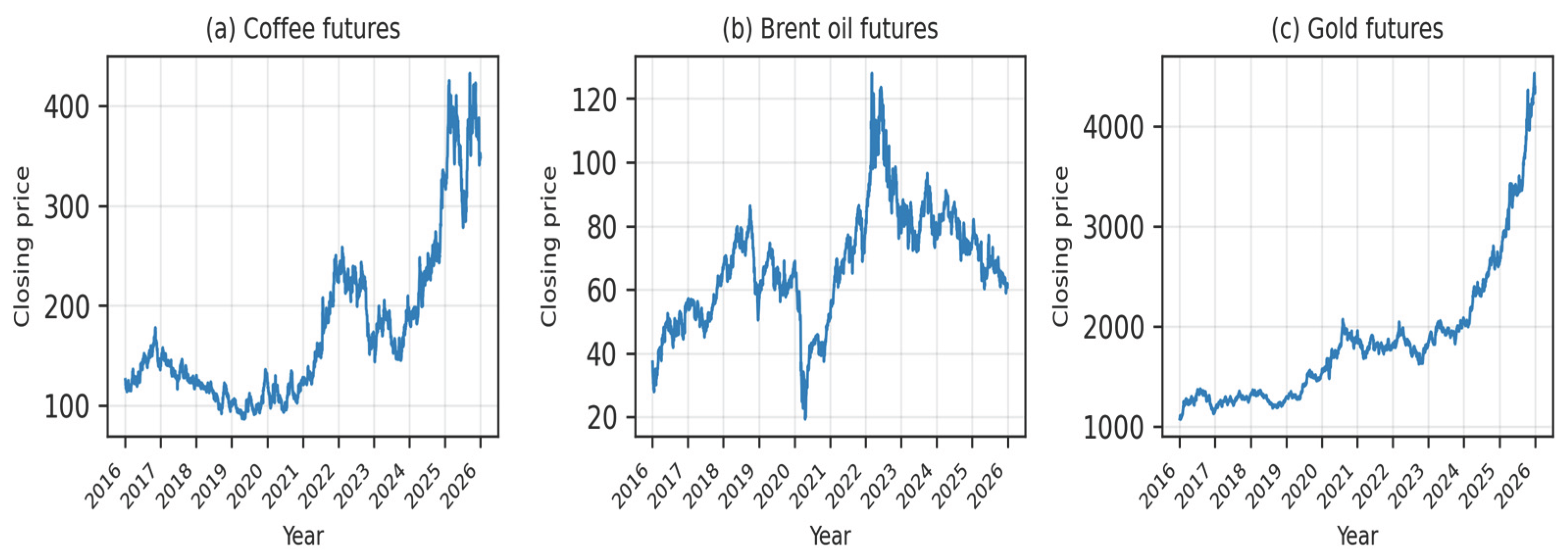
Figure 2.
Base-100 price index by commodity: (a) coffee; (b) Brent oil; (c) gold.
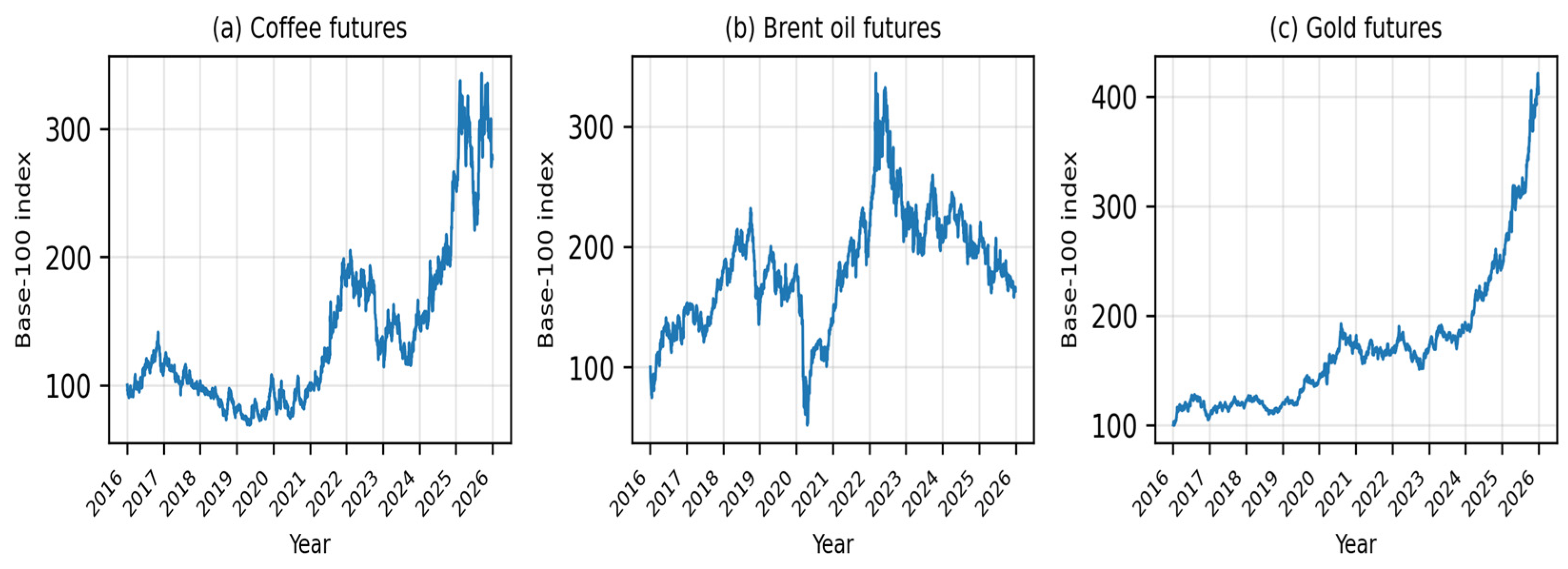
Figure 3.
Empirical distribution of logarithmic returns: (a) coffee; (b) Brent oil; (c) gold.
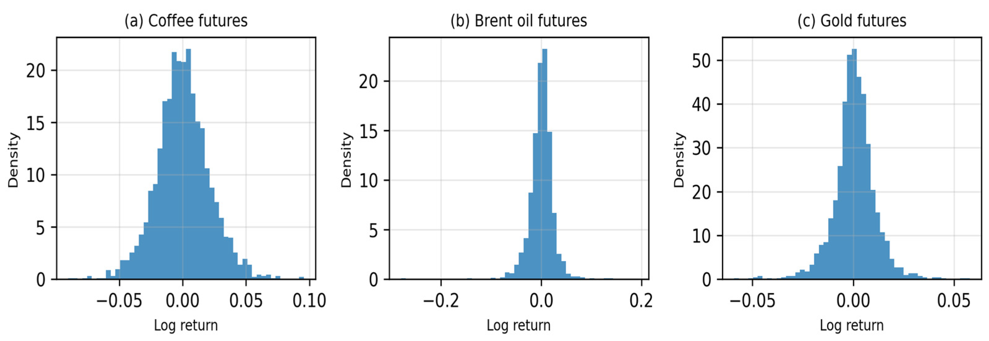
Figure 4.
30-day annualized rolling volatility: (a) coffee; (b) Brent oil; (c) gold.
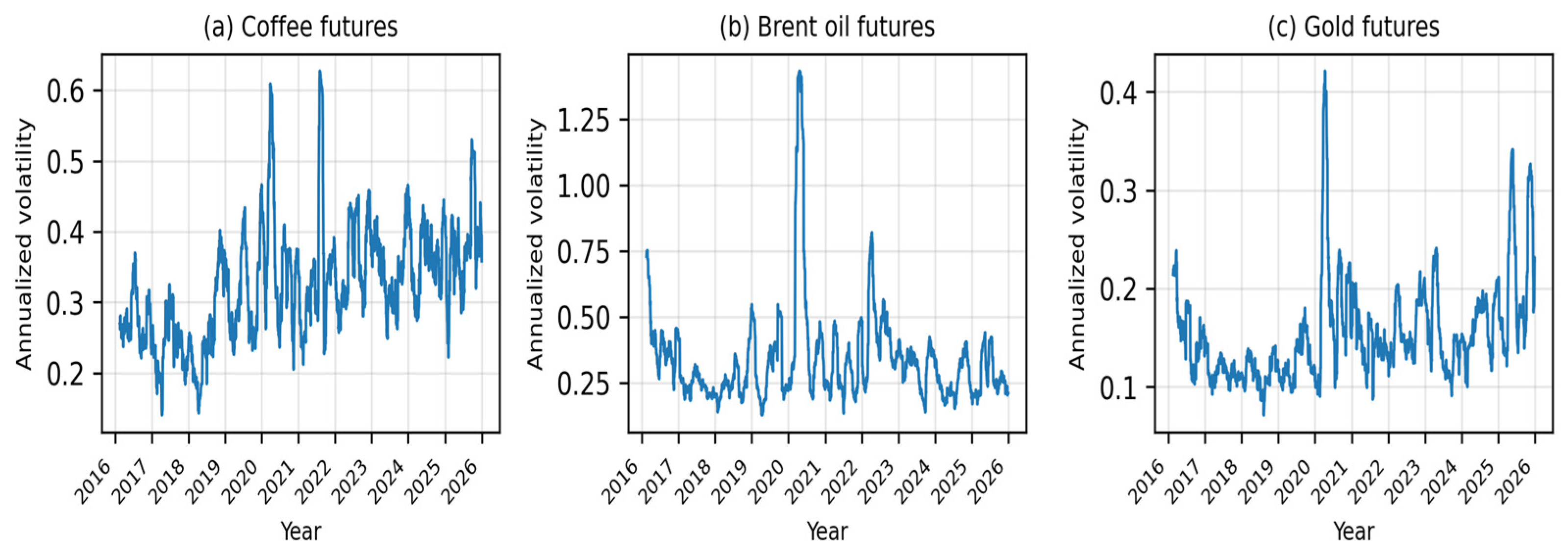
Figure 5.
Autocorrelation of returns and squared returns: (a) coffee; (b) Brent oil; (c) gold.
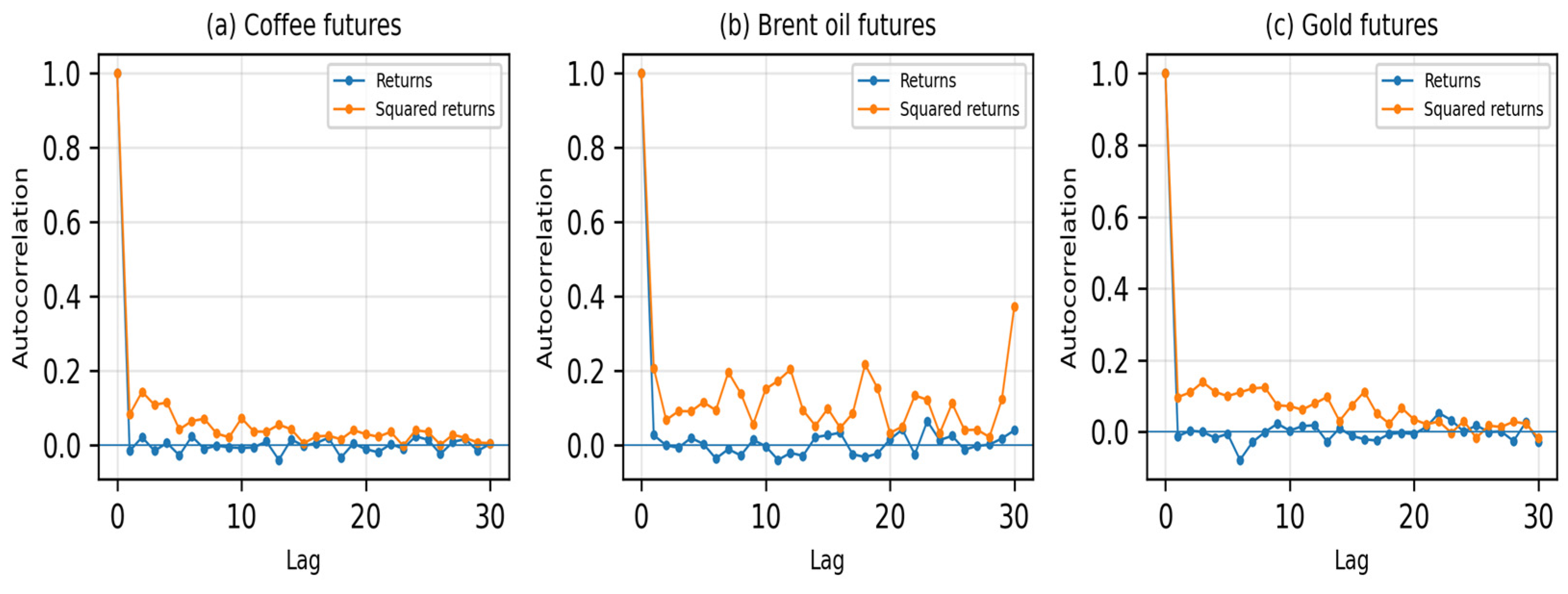
Figure 6.
DFA scaling curves on a log-log scale: (a) coffee; (b) Brent oil; (c) gold.
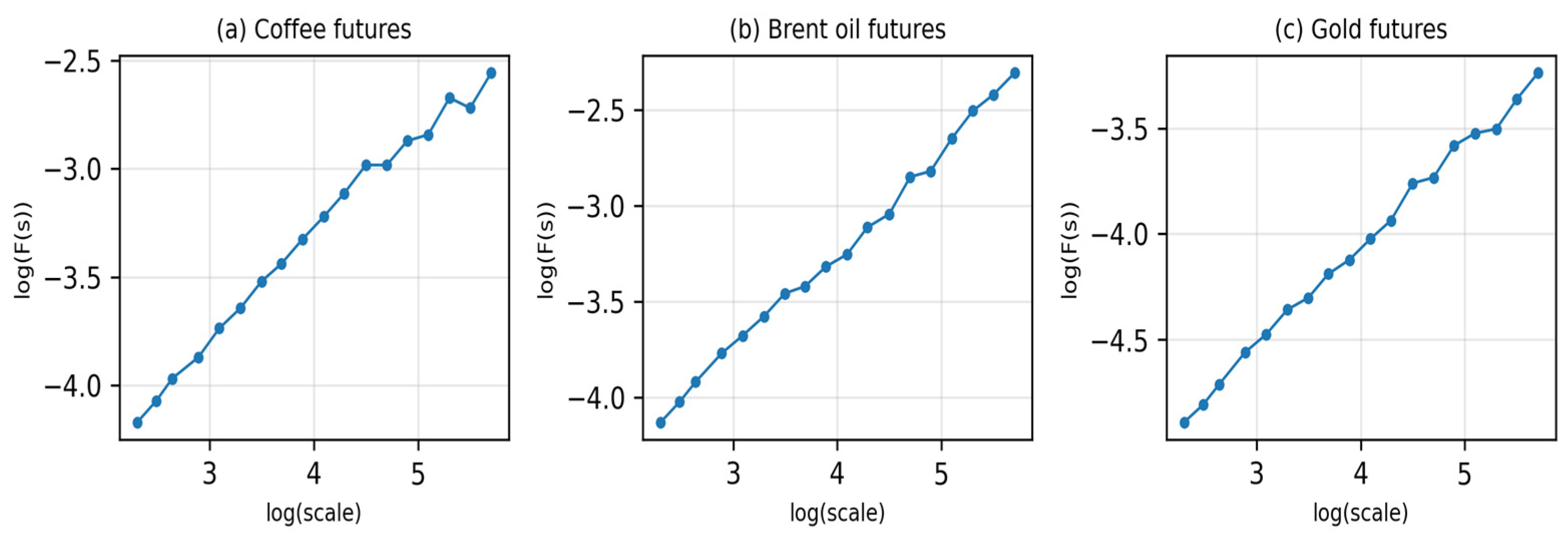
Figure 7.
Generalized MF-DFA functions: (a) coffee; (b) Brent oil; (c) gold.
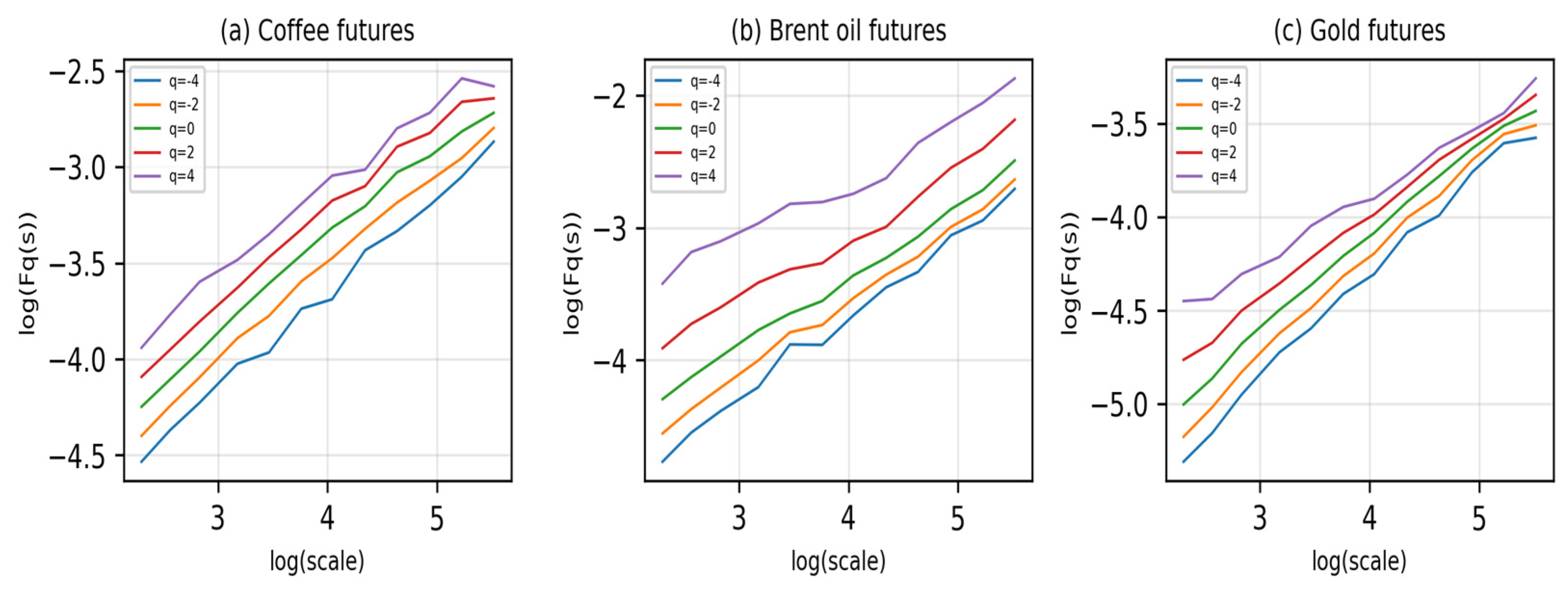
Figure 8.
Monte Carlo fan charts with P5-P95 intervals: (a) coffee; (b) Brent oil; (c) gold.
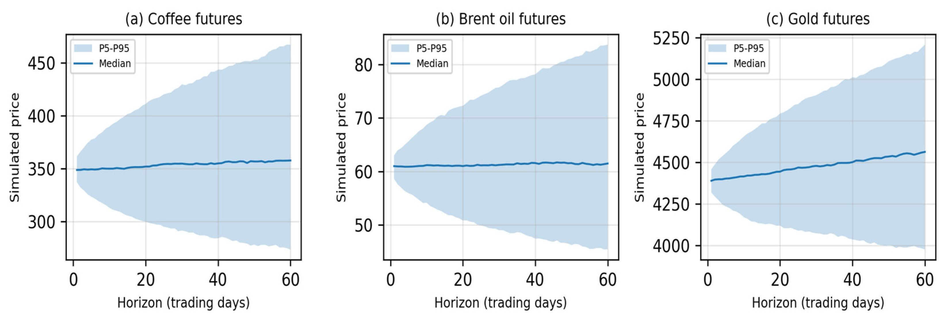

Table 1.
Contract-series definition, source status and empirical scope.
| Commodity | Market segment | Provider label | Contract family | Quotation unit | Source | Empirical treatment | Valid prices | Valid returns |
|---|---|---|---|---|---|---|---|---|
| Coffee | Agricultural commodity | Coffee futures | ICE Coffee C futures family | US cents/lb | Investing.com | Provider-reported historical futures series; no maturity-specific rollover inferred | 2516 | 2515 |
| Brent oil | Energy commodity | Brent oil futures | ICE Brent crude futures family | USD/bbl | Investing.com | Provider-reported historical futures series; no exchange-level contract rule inferred | 2582 | 2581 |
| Gold | Precious metal / safe haven | Gold futures (GC) | COMEX gold futures family | USD/troy oz | Investing.com | Provider-reported historical futures series; calendar irregularity documented | 2188 | 2187 |
Table 2.
Data-quality, source-status and calendar-validation criteria.
| Validation dimension | Field or source | Criterion applied | Interpretive scope |
|---|---|---|---|
| Temporal order | date, commodity | Ascending order within each commodity | Allows returns and rolling measures to be calculated inside each series |
| Duplicate control | date, commodity | No repeated date for the same commodity | Avoids double-counted observations |
| Positive prices | closing_price | Numeric prices greater than zero | Permits logarithmic transformations |
| Return consistency | log_return | Valid returns equal valid prices minus one | Confirms internal arithmetic, not contract continuity |
| Calendar coverage | date | Observed records compared across years | Identifies uneven observation density, especially in gold |
| Source status | provider label | Secondary aggregator explicitly declared | Prevents exchange-certified contract claims |
| Traceability | source, notes | Source and processing notes preserved | Facilitates audit and reuse under stated limitations |
Table 3.
Processed variables and risk-analysis function.
| Variable | Technical definition | Transformation | Analytical role |
|---|---|---|---|
| closing_price | Daily closing price of the reported futures series | Original market record | Market-level trajectory and initial input |
| log_price | Natural logarithm of the closing price | ln(P_i,t) | Scale stabilization and return construction |
| log_return | Continuous relative variation between consecutive prices | ln(P_i,t/P_i,t-1) | Distribution, volatility and tail-risk analysis |
| abs_return | Absolute magnitude of the logarithmic return | |r_i,t| | Intensity of fluctuations and stress episodes |
| squared_return | Squared logarithmic return | (r_i,t)^2 | Second-moment dependence and volatility clustering |
| rolling_volatility_30d | Annualized 30-day rolling volatility | sqrt(252) times 30-day rolling SD | Recent risk and volatility regimes |
| base100_index | Index normalized from the first valid price | P_i,t/P_i,0 x 100 | Relative cumulative comparison across units |
| standardized_return | Return centered and scaled by its own SD | (r_i,t-rbar_i)/s_i | Relative extremes within each commodity |
Table 4.
Calendar coverage and missing-observation profile.
| Commodity | Observed prices | Coverage profile | Largest missing-weekday count | Risk interpretation |
|---|---|---|---|---|
| Coffee | 2516 | Stable annual coverage: 250-253 observations | 10 | Calendar structure supports univariate risk diagnostics |
| Brent oil | 2582 | Stable annual coverage: 257-259 observations | 3 | Most regular series in the sample |
| Gold | 2188 | Reduced coverage in 2017-2019 and 2022-2025 | 64 | Scaling and cross-market comparisons require caution |
Table 5.
Distributional and historical-risk diagnostics of logarithmic returns.
| Commodity | N | Mean | SD | VaR 1% | ES 1% | VaR 5% | ES 5% | Max drawdown | Skew. | Kurt. | JB | Q(20) r2 |
|---|---|---|---|---|---|---|---|---|---|---|---|---|
| Coffee | 2515 | 0.0004 | 0.0210 | -0.0499 | -0.0611 | -0.0337 | -0.0447 | -0.5131 | 0.099 | 3.976 | 103.8 | 200.8 |
| Brent oil | 2581 | 0.0002 | 0.0244 | -0.0673 | -0.1016 | -0.0376 | -0.0585 | -0.7760 | -1.092 | 20.759 | 34428.0 | 899.2 |
| Gold | 2187 | 0.0006 | 0.0103 | -0.0272 | -0.0383 | -0.0164 | -0.0240 | -0.2154 | -0.196 | 6.651 | 1228.6 | 368.7 |
Table 6.
Risk-management interpretation of the empirical evidence.
| Empirical dimension | Main evidence | Risk-management use | Interpretive caution |
|---|---|---|---|
| Return distribution | Non-Gaussian returns and heavy tails | Historical tail-risk monitoring | Not a normal-distribution framework |
| Downside risk | Brent oil has the largest VaR, ES and drawdown | Stress exposure comparison | Historical and unconditional measures |
| Volatility | Time-varying rolling volatility in all series | Identification of stress periods | No dynamic volatility model estimated |
| Second-moment dependence | Q(20) on squared returns exceeds simple-return dependence | Justifies future ARCH/GARCH extensions | Model selection remains future work |
| Scaling | DFA exponents close to 0.5 and structured curves | Exploratory persistence diagnostics | No strong long-memory claim |
| MF-DFA | q-order separation in fluctuation curves | Guides future multifractal testing | Requires spectra, uncertainty and surrogate tests |
| Monte Carlo scenarios | P5-P95 fan charts from empirical bootstrap | Short-horizon uncertainty communication | Not backtested VaR or Expected Shortfall |
Disclaimer/Publisher’s Note: The statements, opinions and data contained in all publications are solely those of the individual author(s) and contributor(s) and not of MDPI and/or the editor(s). MDPI and/or the editor(s) disclaim responsibility for any injury to people or property resulting from any ideas, methods, instructions or products referred to in the content. |
© 2026 by the authors. Licensee MDPI, Basel, Switzerland. This article is an open access article distributed under the terms and conditions of the Creative Commons Attribution (CC BY) license (http://creativecommons.org/licenses/by/4.0/).
Copyright: This open access article is published under a Creative Commons CC BY 4.0 license, which permit the free download, distribution, and reuse, provided that the author and preprint are cited in any reuse.