

Submitted:
07 September 2026
Posted:
09 September 2026
You are already at the latest version
Abstract
This paper examines the mathematical model governing the behavior of a buoyant fluid column rising through a less buoyant ambient fluid within a confined region bounded by two vertical walls. The study represents a bounded-domain extension of the compositional plume model previously developed by Eltayeb and Loper [9 – 11] for an unconfined environment.
The system is characterized by five dimensionless parameters: (i) the Grashoff number, representing the ratio of buoyancy forces generated by concentration differences between the plume and the surrounding fluid to viscous forces; (ii) the Prandtl number, defined as the ratio of viscosity to thermal diffusivity; (iii) the plume thickness; (iv) the separation distance between the two vertical walls; and (v) the dimensionless distance between the plume and the nearest wall, with all length scales normalized using the salt-finger length scale.
The principal aim of the study is to assess how the presence of boundaries modifies the solutions obtained for an unbounded ambient fluid. The analysis shows that the basic-state solution does not depend on either the Grashoff or Prandtl numbers. Unlike the unbounded case, where symmetry is preserved, the presence of sidewalls generally breaks this symmetry unless the plume is positioned exactly midway between the two boundaries.
In an unbounded domain, the plume is always unstable and exhibits two independent modes of instability: the varicose (V) mode and the sinuous (S) mode. The introduction of sidewalls significantly changes the stability characteristics of the flow. A strongly unstable region emerges when a thin plume is located near a boundary. In other areas of the parameter space, the instability growth rate remains comparable to that of the unbounded configuration but decreases as the distance between the walls becomes smaller. Instability continues to appear in two distinct classes of solutions related to the classical varicose and sinuous modes, although these modes are modified by the plume’s position relative to the nearest sidewall.
Keywords:
flow dynamics
; compositional plumes
; hydrodynamic stability
; instability growth rate
; bounded domains
1. Introduction
When a binary fluid consisting of two components with different densities is cooled from below, the component with the higher freezing temperature solidifies first. The resulting solid crystals accumulate at the base of the container, forming a porous layer composed of solid crystals and the remaining lighter fluid [6]. This porous region is commonly referred to as a mushy layer [15]. If the crystallized material corresponds to the denser component, the crystals settle further and create a solid layer beneath the mushy region [4]. As solidification proceeds, the mushy layer increases in thickness and may eventually become unstable [25]. This instability can generate compositional plumes, where the lighter component rises from the mushy layer through the overlying melt [9]. These plumes are examples of directed fluid motion occurring within a surrounding fluid of different composition and physical properties. Such flows are known as compositional plumes (Al Mashrafi & Eltayeb, 2014a).
The mathematical study of compositional plume dynamics is essential for understanding the behavior of fluid mixtures and alloys subjected to thermal and pressure gradients. Such understanding has significant implications in a variety of practical applications, including industrial processes such as metal casting, geophysical phenomena such as solidification at the Earth’s inner core boundary and mantle convection, and environmental processes such as salt-finger formation and sea-ice dynamics.
In industrial applications, one of the challenges encountered in iron casting is the formation of defects known as freckles [21]. During the casting process, trapped gases escape through narrow channels within the molten metal. Upon solidification, these channels appear as thin dark streaks running along the iron bar. The presence of such imperfections can significantly reduce the mechanical strength and structural integrity of the final product.
In geophysical systems, the Earth’s outer core is believed to consist primarily of molten iron and nickel, together with smaller amounts of lighter elements such as sulfur, oxygen, hydrogen, and helium, while the inner core is largely solid iron and nickel [16]. Although temperature generally increases with depth within the Earth, it has been proposed that the inner core continues to grow through solidification occurring at the inner core boundary (ICB) because of extremely high pressures [2,24]. During this process, iron crystallizes while the lighter elements remain in liquid form, leading to the formation of a mushy layer. The dense iron crystals settle onto the ICB, contributing to the gradual growth of the inner core [18]. This mushy layer may become unstable [19], giving rise to narrow ascending columns of light fluid in the form of compositional plumes (Figure 1). These plumes are believed to interact with the Earth’s magnetic field and may play a role in sustaining the geodynamo responsible for generating the planet’s magnetic field [17].
Compositional plumes also occur in environmental settings, particularly in the phenomenon known as salt fingers (Figure 2). In polar and subpolar regions, situations can arise in which relatively warm and fresh water overlies colder and saltier water. Because heat diffuses more rapidly than salt, the upper water layer loses heat faster than it loses salinity [22]. Consequently, the surface water becomes colder while retaining a relatively high salt concentration, increasing its density. The denser fluid then sinks in the form of narrow compositional plumes, creating structures known as salt fingers [14]. This process contributes significantly to heat and salt transport in the oceans and therefore influences climate dynamics in cold regions.
The contrasting effects of compositional plumes in different applications, being detrimental in industrial casting processes while playing beneficial roles in geophysical and environmental systems, have motivated extensive research into their formation, evolution, and stability. Understanding the dynamics of these plumes remains an important objective in fluid mechanics and related scientific disciplines.
The dynamics of compositional plumes have been investigated both theoretically and experimentally. Experimental studies (see Figure 3) suggest that plume flow is generally stable [20], although some experiments have reported unstable behavior [5]. In addition, these studies showed that plume behavior depends on its position within the container, particularly whether it is located near a wall or away from it [13].
On the theoretical side, several studies have been undertaken to investigate the dynamics and stability of compositional plumes. The work of Eltayeb and Loper [9] was the first to examine the stability of compositional plumes. They investigated the stability of vertical interfaces across which an imposed compositional discontinuity existed in the presence of a vertically oriented stabilizing temperature gradient. They subsequently extended their analysis to more realistic plume configurations [10,11] . These studies consistently concluded that compositional plumes are inherently unstable. Furthermore, plume instability has been shown to persist in the presence of rotation [8], magnetic fields [12], and the combined effects of rotation and magnetic fields [7]. However, all these theoretical investigations were conducted in unbounded domains, and material diffusion was assumed to be negligible.
Comparison between theoretical predictions and experimental observations is complicated by differences in the fluid domain surrounding the plume. The present study therefore aims to investigate theoretically the influence of boundaries on plume dynamics. A simplified model is developed that incorporates the principal factors expected to affect the rise of a compositional plume in a bounded domain. The model is illustrated in Figure 4. A vertical column of fluid of finite thickness rises through a surrounding fluid of different compositions and is bounded on either side by rigid vertical walls separated by a distance The coordinate system is chosen such that the plume interfaces are located at while the walls are situated at
2. Formulation of the Model
We consider a two-component incompressible fluid consisting of a solvent (light material) with concentration and temperature . The two constituents are assumed to possess identical kinematic viscosity, , and thermal diffusivity, , while molecular diffusion of the material component is neglected. Following Eltayeb and Loper [9], the fluid motion is described by the governing equations of momentum, mass conservation, heat transfer, concentration transport, and the equation of state.
These equations are
(1)
(2)
(3)
(4)
(5)
Here, denotes the velocity vector, the pressure, the constant gravitational acceleration, the unit vector directed vertically upward, and the time. The parameters and represent the coefficients of thermal and compositional expansion, respectively, while denotes the fluid density. Quantities with the subscript refer to constant reference values. Throughout this study, the fluid is assumed to satisfy the Boussinesq approximation, whereby density variations are neglected in the governing momentum equations except in the buoyancy term, where they contribute to the gravitational force.
Under the Boussinesq approximation, density variations are neglected throughout the governing equations except in the buoyancy term of the momentum equation, where they contribute to the gravitational force. The system admits a hydrostatic equilibrium state. The equations (1) - (5) allow a hydrostatic balance governed by
(6)
Motivated by experimental studies of plumes originating from mushy layers, the temperature distribution is prescribed as
(7)
where is a positive constant. This temperature profile increases with height, producing a thermally stable stratification. Consequently, any instability that develops is expected to arise primarily from compositional effects rather than thermal convection.
To express the governing equations in dimensionless form, appropriate characteristic scales are introduced. Since the focus is on instabilities associated with the ascent of buoyant fluid, the maximum concentration of the light material in the basic state, , is selected as the concentration scale. To preserve the influences of both thermal and compositional stratification, the characteristic temperature scale is chosen such that the thermal and compositional buoyancy contributions remain comparable. Then the unit of temperature is
(8)
Because the observed buoyant plume is narrow, viscous forces must remain of the same order as the buoyancy forces. This requirement leads to the selection of characteristic length and velocity scales based on the classical salt-finger length scale [9,23]. These scales are given by
(9)
The associated convective time scale is then adopted as the relevant timescale for analyzing the growth of instabilities [1].
(10)
A corresponding pressure scale is also introduced as
(11)
Then the governing equations (1) - (5) are subsequently recast in nondimensional form:
(12)
(13)
(14)
(15)
The resulting dimensionless system contains two principal parameters: the Grashoff number and the Prandtl number. The Grashoff number measures the ratio of buoyancy forces generated by
concentration differences between the plume and the ambient fluid to viscous forces, whereas the Prandtl number represents the ratio of momentum diffusivity to thermal diffusivity. These two dimensionless numbers are written in the form
(16)
A Cartesian coordinate system is adopted throughout the study to describe the flow field, with the 𝑧 -axis oriented vertically upward and the 𝑥 - and 𝑦 -axes lying in the horizontal plane. The dependent variables are decomposed into hydrostatic, basic-state, and perturbation components. The hydrostatic contribution accounts for the equilibrium pressure and temperature distributions, while the basic-state variables depend only on the horizontal coordinate 𝑥, representing a steady vertical plume. Small-amplitude perturbations are then introduced into this basic state to investigate its stability characteristics. Then the variables of the system (12) − (15) take the form
(17)
(18)
(19)
(20)
such that the variables with subscript h have hydrostatic contribution and given by
(21)
in which
is a reference value.
The boundary conditions are specified as follows. First, the heat flux, momentum flux, and all flow variables except concentration are continuous across the plume interfaces. Second, the bounding walls are rigid and maintained at the hydrostatic temperature distribution. Third, the plume interfaces are treated as material surfaces. Since material diffusion is assumed negligible, no transfer of light material occurs across these interfaces, consistent with the analysis of Al Mashrafi and Eltayeb [1].
Substituting the decomposed variables (17) - (20) into the governing equations (12) - (15) and collecting terms independent of the perturbation amplitude yields the equations governing the basic state. These equations are given by
(22)
(23)
Retaining terms proportional to the perturbation amplitude of order produces the linearized perturbation equations. These equations form the basis of the stability analysis that are used to determine the behavior and growth of disturbances within the plume. These perturbation equations are
(24)
(25)
(26)
(27)
3. Basic State Solution
The governing equation (15) is identically satisfied by the basic state, allowing the concentration distribution to be specified freely. In this study, a top-hat concentration profile is adopted.
(28)
By introducing the expression
(29)
the governing equations (22) and (23) reduce to
(30)
subject to the boundary conditions
(31)
The solution of the system (28) – (31) is given by
(32)
where and are given by
(33)
The basic-state solution was computed numerically, and representative results are presented in Figure 5 and Figure 6 [1]. Figure 5 demonstrates the influence of the sidewalls on the plume structure. For a plume of fixed thickness, decreasing the separation between the sidewalls intensifies the plume-induced flow. When the plume is positioned closer to one wall than the other, the downward flow outside the plume becomes weaker in the region adjacent to the nearest wall and stronger on the opposite side. As a result, the flow field loses its symmetry.
Figure 6 highlights the effect of plume thickness and wall proximity on the flow characteristics. The results indicate that the sidewalls exert a significant influence on the solution. When the plume is located at the midpoint between the walls, the profiles remain symmetric. However, this symmetry is progressively disrupted as the plume approaches one of the sidewalls. In addition, the oscillatory behaviour of the velocity field can produce regions of negative velocity, corresponding to downward motion within the plume when the plume thickness is sufficiently large. This phenomenon alters the overall transport of material and affects the net flux carried by the plume.
4. The Stability Analysis
To examine the linear stability of the basic-state solution given by (32) , we use the perturbation equations (24) - (27). The interface located at the plane is assumed to be subjected to a small-amplitude harmonic disturbance, as illustrated in Figure 7, of the form
(34)
where and denote the horizontal and vertical wavenumbers, respectively. The symbol c.c. represents the complex conjugate, while is a constant amplitude parameter that may conveniently be written as
. (35)
This representation enables the disturbance field to be expressed as a normal-mode solution, thereby facilitating the analysis of the growth or decay of perturbations and the determination of the stability characteristics of the basic flow.
The real component controls the temporal evolution of the disturbance amplitude and, consequently, determines its stability characteristics. When the real part remains negative for all possible combinations of wavenumbers and , the plume is considered stable. In contrast, the plume becomes unstable if at least one combination of wavenumbers and produces a positive value. A neutrally stable state exists when the real part is zero for all wavenumber values.
If the most amplified mode is associated with both wavenumbers and being non-zero, the disturbance is classified as a three-dimensional (3D) mode. When , the disturbance is referred to as a two-dimensional (2D) mode. The situation in which and is not observed. The imaginary component , on the other hand, governs the propagation of the disturbance by determining its phase velocities. The vertical phase speed and the horizontal phase speed are defined as follows.
(36)
It should be noted that is defined only when .
The disturbance (34) propagates through the fluid, influencing the second interface and inducing perturbations in the system variables. As a result, the interface located at can be expressed in the form
(37)
where represents the amplitude of the interface displacement, as determined by the boundary conditions of the problem, while the perturbation variables can be expressed in the form
(38)
where the factors are introduced into the variables and respectively, for notational convenience.
Substituting the expressions given by (39) into Equations (24) – (27) yields the following system of ordinary differential equations in the variable
(40)
(41)
(42)
(43)
(44)
(45)
where
(46)
It is convenient to derive the following three equations
(47)
(48)
(49)
The first equation (47) is obtained by differentiating (50) with respect to and subsequently subtracting (51). The second equation (52) is derived by differentiating (53) once and then subtracting (54). The third equation (55) is obtained by applying the operator to (56) and making use of Equations (40) - (57). The variable , which is associated with the vertical component of the vorticity, is defined by
(58)
It follows from this equation (59) that the perturbation concentration vanishes everywhere within the fluid domain. Consequently
(60)
The system is subject to the following boundary conditions
(61)
(62)
(63)
(64)
where denotes the operator defined by
(65)
representing the discontinuity, or jump, across . It should be noted that the governing equation (66)has been used to replace the continuity condition on together with its vanishing at the boundaries by the condition , since is likewise continuous across the interfaces and vanishes at the boundaries. The jump conditions (67) express the requirement that the interfaces behave as material surfaces.
Earlier studies on compositional plumes have shown that the flow is unstable when the Grashoff number, is small [10]. Since the Grashoff number measures the strength of the plume through the maximum amplitude of the basic concentration distribution, instability at small implies instability throughout the entire range of possible values. Accordingly, the variables of the system and may be expanded in powers of the small parameter in the form
(68)
where stands for any of the perturbation variables , , , or .
Upon substituting the expansion (69) into Equations (40) - (44), (47) - (49) and the associated boundary conditions (61) - (64) , and requiring the coefficients of ( = 0 , 1 , 2 , ….) to vanish independently, a sequence of ordinary differential equation systems is obtained. Solving these systems successively provides the expression for the growth rate. To leading order, the stability characteristics of the interfaces are determined by the two systems corresponding to (hereafter referred to as Problem 0) and (hereafter referred to as Problem 1).
4.1. Problem 0
The coefficients of in the system of R0 in the system of equations (42) − (44), (47) − (49) are given as follows
(70)
(71)
(72)
(73)
(74)
(75)
subject to the following boundary conditions
(76)
(77)
(78)
(79)
The system, (70) - (75) subject to the prescribed boundary conditions, can be solved directly using the elimination method to determine the unknown variables. Subsequently, applying the boundary conditions (79) yields expressions for the growth rate and the interface displacement [1]. This results in the following expression
(80)
(81)
where
(82)
(83)
(84)
(85)
with
(86)
with representing the three roots of the cubic equation
(87)
The nature of the roots of the cubic equation (87) ensures that the relevant expressions and are real. Consequently, the quantities and are real , implying that the discriminant appearing in the equation (80) is also real. When the discriminant is positive, the equation admits two distinct real roots; when it vanishes, the roots are real and identical. In both cases, is purely imaginary, indicating that the system is neutrally stable. Therefore, it is necessary to proceed to the next-order approximation (Problem 1). Here, is given by
(88)
where the superscripts and are used to distinguish between the two modes.
When the discriminant is negative, the equation possesses a pair of complex-conjugate roots. Consequently, the corresponding values of have real parts with opposite signs. The root associated with the positive real part characterizes the unstable mode of the system. The two roots can be expressed as follows:
(89)
Using the expression (81), the amplitudes and can be expressed as
(90)
In the absence of sidewall boundaries, the two modes correspond to configurations in which the plume interfaces oscillate either in phase, resulting in a sinuous mode, or out of phase, resulting in a varicose mode (see Figure 8). In both cases, is purely imaginary, implying that the disturbances are neutrally stable at the present order of approximation. The introduction of sidewalls breaks this symmetry, except in the special case where the plume is positioned equidistantly between the boundaries. However, when the discriminant is real, both modes remain neutrally stable and propagate with distinct phase speeds while retaining either an in-phase or an out-of-phase structure. By contrast, when the discriminant is negative, the plume becomes unstable and assumes complex values. Consequently, a phase difference arises between the two interfaces, such that they exhibit neither an in-phase nor an out-of-phase relationship.
It follows from the governing equations (89) that, if one of the two modes exhibits a positive growth rate, the other must necessarily possess a negative growth rate. Consequently, at most one of the modes can be unstable. Since , the MS mode is identified as the unstable mode. Figure 9 illustrates the behaviour of the MS mode in the wavenumber plane for representative values of . It is evident that, as the plume thickness decreases, the region of the wavenumber plane corresponding to instability expands, although the maximum growth rate is reduced. Conversely, as the plume becomes thicker, the unstable region contracts and eventually vanishes when exceeds . The instability is characterized by a two-dimensional mode, and the vertical wavenumber decreases with increasing .
in the plane for . Results are shown for = (a) , (b) , (c) , and (d) . Instability occurs within the contour, while the flow remains neutrally stable outside the curve .
The preferred instability mode is identified as the one corresponding to the maximum growth rate (76) as a function of the wavenumbers and for fixed values of the parameters , and . In other words, we solve the governing differential equations and determine the mode that exhibits the largest growth rate:
(91)
Maximization of the growth rate (89) reveals that instability occurs only for the MS mode when . Furthermore, the unstable mode is two-dimensional and propagates vertically upwards .
A representative set of profiles for the preferred mode is presented in Figure 10. The growth rate increases from zero at the boundary, reaches a maximum at a certain distance from the wall, and subsequently decreases. This distance depends on both the plume thickness and the parameters . The vertical wavenumber, , decreases as the plume moves away from the wall when the plume is sufficiently thin; however, for relatively thick plumes exhibit the opposite behavior and increases with distance from the wall.
The instability region in the plane is illustrated in Figure 11. It can be observed that the unstable region expands with increasing plume thickness, reaches a maximum extent, and then gradually shrinks as the plume thickness approaches zero. In general, the plume remains neutrally stable throughout the domain, except in the case of very thin plumes located close to the wall, where instability may arise. We next investigate the stability characteristics of Problem 1.
plane, corresponding to growth rates of order . The region marked represents neutral stability, while the region marked indicates the onset of instability. In all unstable cases, the preferred mode is the modified sinuous (MS) mode; the modified varicose (MV) mode is found to be stable.
4.2. Problem 1
The coefficients associated with the perturbation terms of in the governing equations yield the following set of equations
(92)
(93)
(94)
(95)
(96)
(97)
(98)
where we have defined the expressions
(99)
The governing equations are subject to the following boundary conditions
(100)
(101)
(102)
The governing equations, together with the boundary conditions (92) - (102), can be solved by deriving the solvability condition for the resulting nonhomogeneous system[1]. This analysis yields an expression for the growth ratewhich may be written in the form
(103)
In the above expression, takes the modes or , corresponding to the sinuous and varicose modes, respectively. The quantities , , , and are given by the following integrals:
(104)
(105)
(106)
(107)
(108)
where , , , , , are specified as follows
(109)
(110)
(111)
(112)
(113)
(114)
and , , and are
(115)
(116)
(117)
(118)
The growth rate defined by (103), can be decomposed into five distinct contributions, each
reflecting the influence of specific system parameters and variables. The terms and arise
from interactions between the perturbation variables and the growth rate of the leading-order system,
whereas and result from interactions between the leading-order variables and the basicstate
quantities. While and are independent of the Prandtl number, and depend linearly on The term represents the contribution induced by the presence of
boundaries. Since the leading-order variables are real and the first-order variables are imaginary, the
resulting growth rate is purely real and therefore governs the amplification or decay of the
disturbance.
Numerical computations of the growth rate (103) indicate that the plume is unstable, with disturbances growing at a rate of. For a given location in parameter space , the preferred mode, corresponding to the maximum growth rate, may be either the modified sinuous (MS) mode or the modified varicose (MV) mode, depending on the complex interplay among the governing parameters. When one parameter is varied while the remaining two are held fixed, a transition in the preferred mode may occur, with the dominant instability changing from MS to MV, or vice versa, once a critical parameter value is reached.
Furthermore, variations in a parameter can cause a mode of a given type, whether MS or MV, to undergo a transition between two-dimensional and three-dimensional structures, or conversely, as the parameter passes through a critical threshold. This behavior arises because the growth-rate expression (103) may possess multiple local maxima. As the parameter increases, the initially dominant maximum may decrease while a secondary maximum increases, until a crossover point is reached at which the latter exceeds the former and becomes the preferred mode. Figure 12 illustrates a representative example of this behavior for a selected set of parameter values.
, = 10 , , and for (a), (b) and for (c), (d). Note that the MS mode is preferred for and the MV mode is preferred when .
Figure 13 illustrates the dependence of the preferred instability mode on the Prandtl number, , and facilitates comparison with the limiting case in which sidewalls are absent. For low values of , the modified sinuous (MS) mode is the preferred mode of instability, whereas the modified varicose (MV) mode becomes dominant as increases. This behavior is consistent with the unbounded configuration reported by Eltayeb and Loper [10]. The critical Prandtl number, , at which the preferred mode switches from MS to MV depends on the distance between the plume and the nearest sidewall. As the wall approaches the plume, increases, indicating that the presence of sidewall boundaries suppresses the MV mode relative to the MS mode. The boundaries also exert a stabilizing influence on the plume, as evidenced by the reduction in the magnitude of the growth rate with decreasing wall separation . It is noteworthy that, regardless of the values of the governing parameters and , the preferred MS mode remains three-dimensional, whereas the preferred MV mode remains two-dimensional when the plume is located midway between the two sidewalls.
, for , when the plume is positioned midway between the two sidewalls . Curves (i) and (ii) correspond to two different sidewall spacings: (i) and (ii) . The solid curve represents the modified sinuous (MS) mode, whereas the dashed curve represents the modified varicose (MV) mode.
In contrast to the unbounded plume, which is unstable of , the bounded Cartesian plume exhibits two distinct instability regimes, characterized by growth rates of orders and. The region associated with the larger growth rate, , occupies only a small portion of the parameter space and is strongly influenced by the spacing of the sidewalls. The corresponding regime diagram is presented in Figure 14 for . Instability with growth rate occurs only when the plume is relatively thin, with a thickness not exceeding approximately one-half of the salt-finger length scale, and when its distance from the nearest sidewall is less than about 0.25. Furthermore, as the plume approaches the wall, the growth rate decreases, indicating that the stabilizing influence of the boundary becomes increasingly significant in the immediate vicinity of the sidewall.
plane for . In panel (a), the regions labeled and correspond to instabilities with growth rates of order and , respectively. The shaded area lies outside the physically admissible domain, since cannot exceeds . Panel (b) presents an enlarged view of the region and from panel (a).
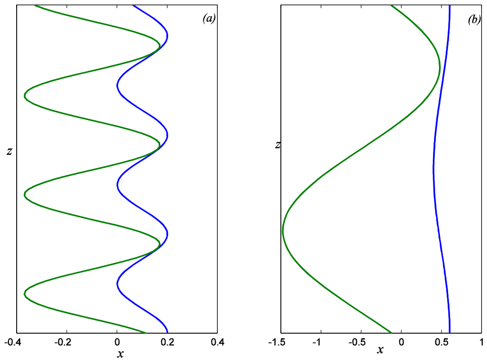
The preferred mode of instability is associated with plume interfaces represented by (34) and (37). The amplitude at the interface is fixed at unity, whereas the amplitude at governed by the ratio , whose value is determined by the parameters defining the preferred mode for given values of . Sample interface profiles for selected preferred modes are displayed in Figure 15. It is observed that the interfaces approach each other closely at periodically spaced positions along the plume, suggesting the possibility of plume breakup and the subsequent formation of discrete blob-like structures.
at . For visual clarity, both profiles are displayed using the same magnification factor (. (a) , , and (b) , , . Notice that the interfaces come into close proximity at periodically recurring positions along the domain.
5. Conclusions
The mathematical model describing the dynamics of bounded Cartesian plumes has been investigated. This study investigates the dynamics of compositional plumes in fluids of infinite extent. To gain insight into the influence of lateral boundaries on plume stability and evolution, a simplified Cartesian geometry is employed. The corresponding unbounded configuration was previously examined by Eltayeb and Loper [9,10,11]. This formulation facilitates a direct comparison between plumes evolving in bounded and unbounded domains, thereby highlighting the effects introduced by the presence of boundaries.
The effect of boundaries on the Eltayeb-Loper model is investigated by introducing two vertical sidewalls on either side of the ascending buoyant fluid column. The inclusion of these boundaries introduces two additional dimensionless parameters into the problem: the distance between the sidewalls, , and the distance from the plume to the nearest sidewall, . In the absence of sidewalls, the basic state is symmetric with respect to the axis, measured normal to the plume interfaces. Consequently, the perturbations can be classified into two independent symmetry classes: the even mode, commonly referred to as the varicose (V) mode, and the odd mode, known as the sinuous (S) mode. The introduction of sidewalls generally breaks this symmetry whenever the plume is not positioned equidistantly between the boundaries. Nevertheless, the two classes of disturbances persist and are subsequently identified as the modified varicose (MV) mode and the modified sinuous (MS) mode.
The presence of sidewalls alters the basic state of a bounded Cartesian plume, with its behavior strongly influenced by the distance between the plume and the nearest boundary. As a result, the stability characteristics of the bounded plume differ significantly from those of its unbounded counterpart. The stability analysis reveals the emergence of a new instability mode when the plume is located sufficiently close to a sidewall. Unlike the unbounded case, where the growth rate scales as the order of magnitude of the growth rate in the bounded configuration depends on both the plume thickness and its proximity to the nearest wall. When the plume is thin and situated close to a boundary, the instability develops with a growth rate of . For other combinations of plume thickness and distance from the nearest sidewall, the plume remains unstable with a growth rate of the same order as that observed in the absence of boundaries. Nevertheless, even in this regime, the magnitude of the growth rate decreases as the separation between the sidewalls becomes smaller.
References
- Al Mashrafi, K.S.; Eltayeb, I.A. The influence of boundaries on the stability of compositional plumes. Open J. Fluid Dyn. 2014a, 4, 83–102. [Google Scholar]
- Braginsky, S. I. Structure of the F-layer and reasons for convection in the Earth’s core. Dokl. Akad. Nauk SSSR 1963, 149, 8–10. [Google Scholar]
- Buffett, B. A. 2007 Geophysics: Taking earth’s temperature. Science 315(5820), 1801–1802. [CrossRef] [PubMed]
- Chen, C. F.; Chen, F. Experimental study of directional solidification of aqueous ammonium chloride solution. J. Fluid Mech. 1991, 227, 567–586. [Google Scholar] [CrossRef]
- Classen; Heimpel, S.; Christensen, M.U. 1999 Blob instability in rotating compositional convection. Geophys. Res. Lett. 26:1, 135–138. [CrossRef]
- Copley, S. M.; Giamei, A. F.; Johnson, S. M.; Hornbecker, M. F. 1970 The origin of freckles in unidirectionally solidified castings. Metall. Trans. 1, 2193–2204. [CrossRef]
- Eltayeb, I.A. 2006 The stability of a compositional plume rotating in the presence of a magnetic field. Geophys. Astrophys. Fluid Dynam. 100, 429–455. [CrossRef]
- Eltayeb, I. A.; Hamza, E. A. 1998 Compositional convection in the presence of rotation. J. Fluid Mech. 354, 277–299. [CrossRef]
- Eltayeb, I. A.; Loper, D. E. On the stability of vertical double-diffusive interfaces. Part1. A single plane interface. J. Fluid Mech. 1991, 228, 149–181. [Google Scholar] [CrossRef]
- Eltayeb, I. A.; Loper, D. E. On the stability of vertical double-diffusive interfaces. Part2. Two parallel interfaces. J. Fluid Mech. 1994, 267, 251–271. [Google Scholar] [CrossRef]
- Eltayeb, I. A.; Loper, D. E. On the stability of vertical double-diffusive interfaces. Part3. Cylindrical interfaces. J. Fluid Mech. 1997, 353, 45–66. [Google Scholar] [CrossRef]
- Eltayeb, I. A.; Hamza, E. A.; Jervase, J. A.; Krishnan, E. A.; Loper, D. E. 2005 Compositional convection in the presence of a magnetic field. II. A Cartesian plume. Proc. R. Soc. Lond. A 461, 2605–2633. [CrossRef]
- Hellawell, A.; Sarazin, J. R.; Steube, R. S. 1993 Channel convection in partly solidified systems. Phil. Trans. R. Soc. Lond. A345, 507–544. [CrossRef]
- Howard, L. N.; Veronis, G. 1992 Stability of salt fingers with negligible diffusivity. J. Fluid Mech. 239, 511–522. [CrossRef]
- Huppert, H. E. The fluid mechanics of solidification. J. Fluid Mech. 1990, 212, 209–240. [Google Scholar] [CrossRef]
- Loper, D. E. The gravitationally powered dynamo. Geophys. J. R. Astron. Soc. 1978, 54, 389–404. [Google Scholar] [CrossRef]
- Loper, D.E.; Roberts, P.H. On the motion of an iron-alloy core containing a slurry. I. Geophys. Astrophys. Fluid Dyn. 1978, 9, 289–321. [Google Scholar] [CrossRef]
- Loper, D. E.; Roberts, P. H. A study of conditions at the inner core boundary of the Earth. Phys. Earth Plan. Int. 1981, 24, 302–307. [Google Scholar] [CrossRef]
- Moffatt, H. K. Liquid metal MHD and the geodynamo. In Liquid Metal Magneto-hydromagnetics; Lielpeters, J., Moreau, R., Eds.; Kluwer: Dordecht, 1989; pp. 403–412. [Google Scholar]
- Sample, A. K.; Hellawell, A. The mechanisms of formation and prevention of channel segregation during alloy solidification. Metall. Trans. 1984, A 15A, 2163–2173. [Google Scholar] [CrossRef]
- Smeltzer, C. E. 1959 Solve Steel “ freckle” Mystery. Iron Age 184, 188–189.
- Stern, M. E. The “salt fountain” and thermohaline convection. Tellus 1960, 12, 172–175. [Google Scholar] [CrossRef]
- Turner, J. S. 1973 Buoyancy Effects in Fluids; Cambridge University Press: Cambridge, U.K.
- Verhoogen, J. 1961 Heat balance of the Earth’s core. Geophys. J. R. Astron. Soc. 4, 276–281.
- Worster, M. G. Instabilities of the liquid and mushy regions during solidification of alloys. J. Fluid Mech. 1992, 237, 649–669. [Google Scholar] [CrossRef]
Figure 1.
Schematic diagram of the solidification at inner core boundary of Earth. A mushy layer of thickness, nearly 1 kilometer, appears at ICB (and it is very thin so that it cannot be seen at this level of resolution). Note that the temperature and pressure are very high at ICB. (Source: [3]).
Figure 1.
Schematic diagram of the solidification at inner core boundary of Earth. A mushy layer of thickness, nearly 1 kilometer, appears at ICB (and it is very thin so that it cannot be seen at this level of resolution). Note that the temperature and pressure are very high at ICB. (Source: [3]).
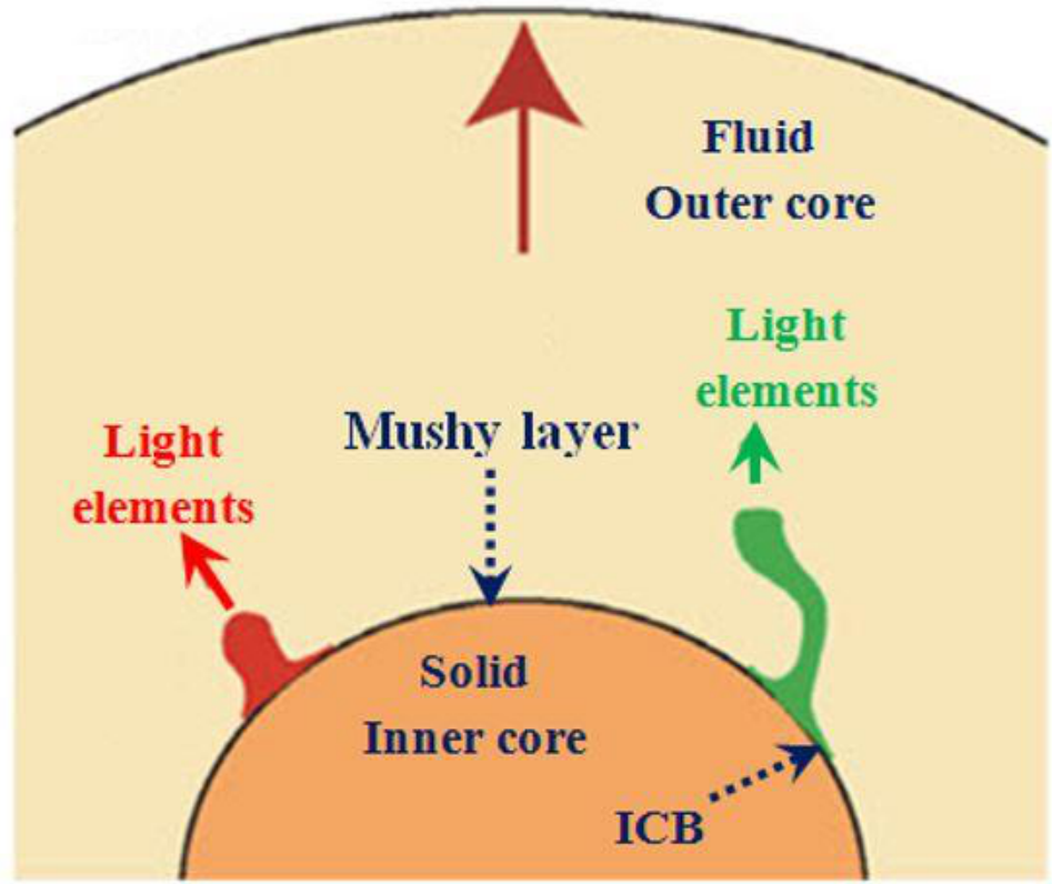
Figure 2.
Schematic diagram of salt finger development. Note that the diffusion of heat must be faster than the diffusion of salt for salt fingers to form.
Figure 2.
Schematic diagram of salt finger development. Note that the diffusion of heat must be faster than the diffusion of salt for salt fingers to form.
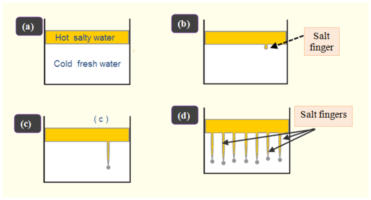
Figure 3.
Aqueous ammonium chloride solution ( a. the experiment by Huppert [15] ; b. the experiment by Eltayeb and Loper [9]).
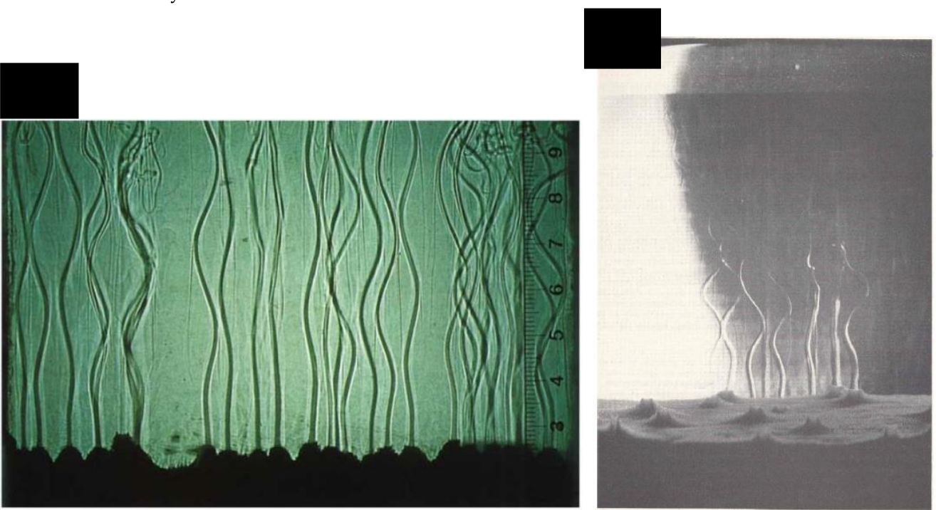
Figure 4.
The geometry of the problem showing the profile of the basic state concentration of light material representing a plume of width,
Figure 4.
The geometry of the problem showing the profile of the basic state concentration of light material representing a plume of width,
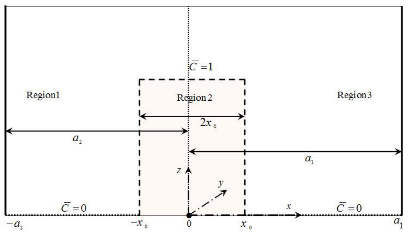
Figure 5.
The profiles of and for and different values of and . The subplots (a) and (c) refer to and when the plume is equidistant from the sidewalls and the labels i, ii, iii correspond to , respectively. The subplots (b) and (d) refer to and when , and labels , , correspond to .
Figure 5.
The profiles of and for and different values of and . The subplots (a) and (c) refer to and when the plume is equidistant from the sidewalls and the labels i, ii, iii correspond to , respectively. The subplots (b) and (d) refer to and when , and labels , , correspond to .
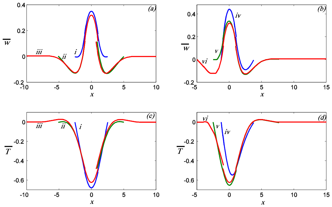
Figure 6.
The profiles of and , for different values of plume thickness, , and distance, , from the sidewall on the left when . The subplots (a) and (c) refer to and when the plume is positioned half-way between the two sidewalls and the labels i, ii, iii correspond to , respectively. The subplots (b) and (d) refer to and when and the labels iv, v, vi correspond to , respectively.
Figure 6.
The profiles of and , for different values of plume thickness, , and distance, , from the sidewall on the left when . The subplots (a) and (c) refer to and when the plume is positioned half-way between the two sidewalls and the labels i, ii, iii correspond to , respectively. The subplots (b) and (d) refer to and when and the labels iv, v, vi correspond to , respectively.
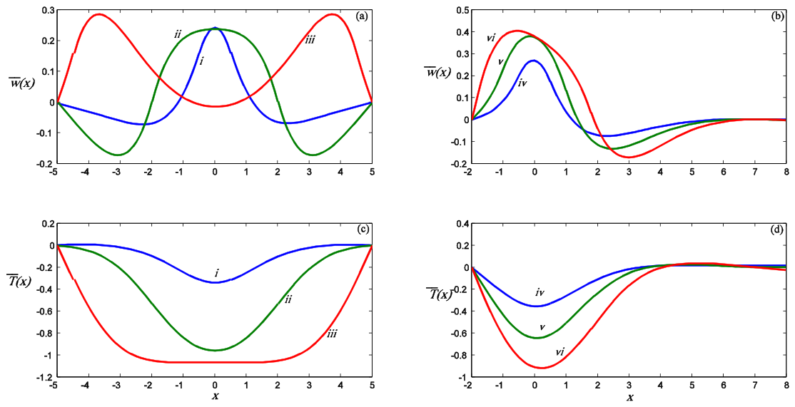
Figure 7.
Illustration of the disturbances of the interfaces. Here , and concentration, 1 , rising vertically in a rotating finite fluid of width, , and concentration , 0. The plume is bounded by two rigid vertical planes on either side such that the center of the plume is a distance from the wall on the right and from the wall on the left.
Figure 7.
Illustration of the disturbances of the interfaces. Here , and concentration, 1 , rising vertically in a rotating finite fluid of width, , and concentration , 0. The plume is bounded by two rigid vertical planes on either side such that the center of the plume is a distance from the wall on the right and from the wall on the left.
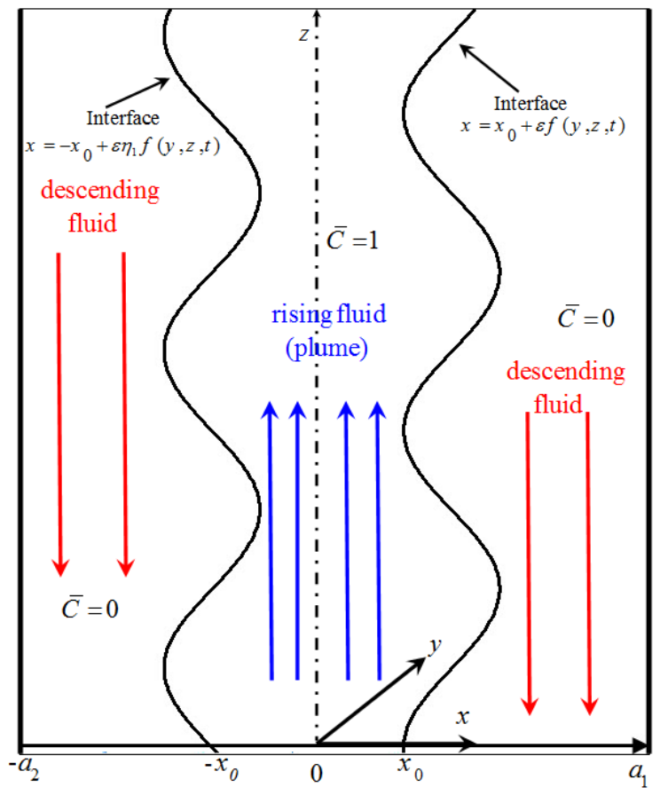
Figure 8.
Schematic illustration of the two interface modes in the absence of boundaries. In this case, the flow exhibits symmetry between the sinuous and varicose modes. The presence of sidewall boundaries breaks this symmetry, except when the plume is located midway between the two sidewalls. The resulting modes are referred to as the modified sinuous (MS) mode and the modified varicose (MV) mode.
Figure 8.
Schematic illustration of the two interface modes in the absence of boundaries. In this case, the flow exhibits symmetry between the sinuous and varicose modes. The presence of sidewall boundaries breaks this symmetry, except when the plume is located midway between the two sidewalls. The resulting modes are referred to as the modified sinuous (MS) mode and the modified varicose (MV) mode.
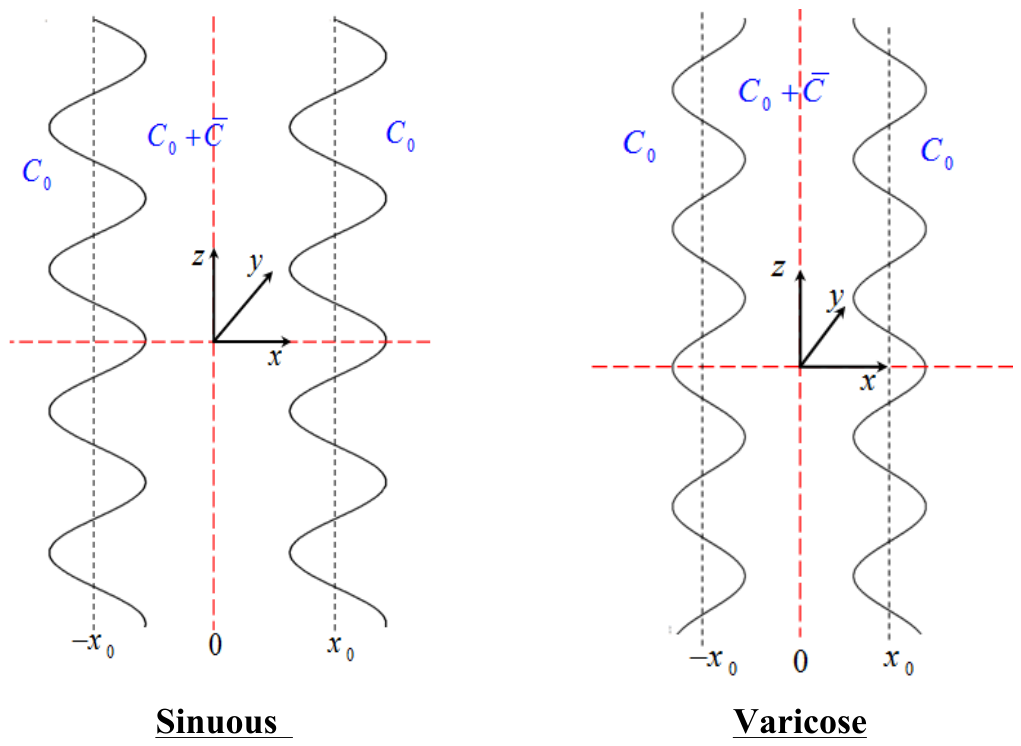
Figure 9.
Growth-rate contours of the modified sinuous (MS) mode
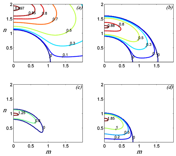
Figure 10.
Profiles of the preferred instability mode correspond to the modified sinuous (MS) mode. The growth rate of order , is plotted as a function of for four values of : 0.1, 0.2, 0.3, and 0.4, with .
Figure 10.
Profiles of the preferred instability mode correspond to the modified sinuous (MS) mode. The growth rate of order , is plotted as a function of for four values of : 0.1, 0.2, 0.3, and 0.4, with .
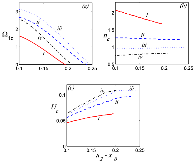
Figure 11.
Stability regime diagram for the bounded Cartesian plume in the
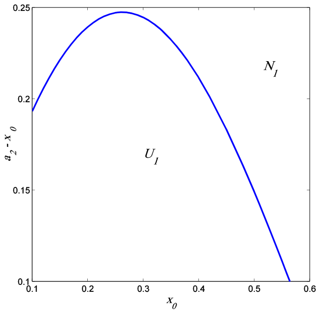
Figure 12.
Growth-rate contours for the modified varicose (MV) and modified sinuous (MS) modes. Panels (a) and (c) depict the MV mode, while panels (b) and (d) depict the MS mode. The calculations are performed for
Figure 12.
Growth-rate contours for the modified varicose (MV) and modified sinuous (MS) modes. Panels (a) and (c) depict the MV mode, while panels (b) and (d) depict the MS mode. The calculations are performed for
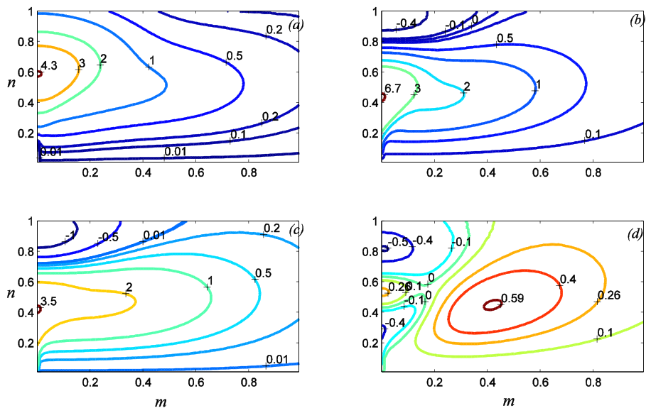
Figure 13.
Illustration of the influence of sidewall boundaries on the stability of the Cartesian plume. The preferred instability mode is shown as a function of the Prandtl number,
Figure 13.
Illustration of the influence of sidewall boundaries on the stability of the Cartesian plume. The preferred instability mode is shown as a function of the Prandtl number,
Figure 14.
Regime diagram of the bounded plume in the
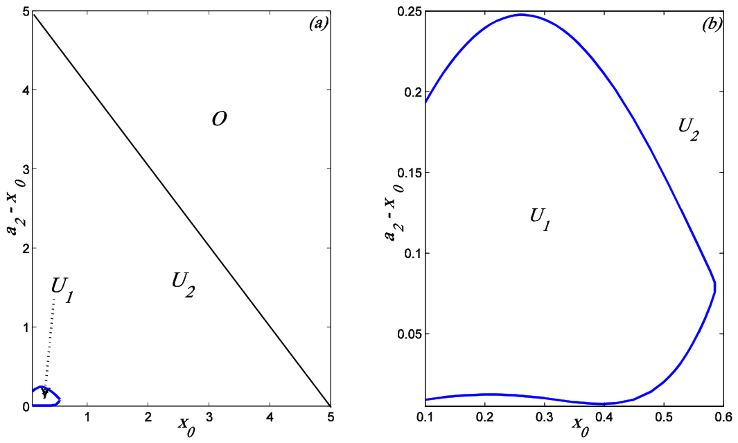
Figure 15.
Profiles of the interfaces corresponding to the unstable mode for two representative parameter values of
Figure 15.
Profiles of the interfaces corresponding to the unstable mode for two representative parameter values of
Disclaimer/Publisher’s Note: The statements, opinions and data contained in all publications are solely those of the individual author(s) and contributor(s) and not of MDPI and/or the editor(s). MDPI and/or the editor(s) disclaim responsibility for any injury to people or property resulting from any ideas, methods, instructions or products referred to in the content. |
© 2026 by the authors. Licensee MDPI, Basel, Switzerland. This article is an open access article distributed under the terms and conditions of the Creative Commons Attribution (CC BY) license (http://creativecommons.org/licenses/by/4.0/).
Copyright: This open access article is published under a Creative Commons CC BY 4.0 license, which permit the free download, distribution, and reuse, provided that the author and preprint are cited in any reuse.