

Submitted:
07 September 2026
Posted:
08 September 2026
You are already at the latest version
Abstract
Traditional credit risk assessment commonly treats borrowers as independent tabular records, overlooking shared geographic and occupational stress that can produce correlated repayment outcomes. We present a reproducible socio-spatial dataset benchmark and testbed for explainable default risk prediction that represents borrowers as nodes in a structured relational network. The benchmark constructs weighted homophily links from observable pre-target attributes and derives structural centrality, community, and multi-hop neighborhood-stress features. A multi-head Graph Attention Network (GAT) learns relational representations that are exported to a downstream tree-based classifier, allowing graph signals to be compared with individual borrower attributes. We evaluate logistic, ensemble, graph feature proxy, and full graph feature models under a stratified protocol, and use ablation analysis to examine the contribution of relational information. The testbed provides a larger-scale experimental framework for studying graph construction, relational representation learning, downstream risk classification, explainability, and computational growth under a common reproducible pipeline. The framework also combines SHAP feature-group attribution with GAT edge attention to provide complementary global and relational explanations. A scalability analysis studies the computational behavior of the downstream evaluation as the benchmark grows. The results support controlled experiments in relational stress modeling while highlighting the limitations of synthetic data. The benchmark is not intended to establish causal contagion, demographic fairness, or regulatory compliance.
Keywords:
graph neural networks
; financial contagion
; socio-spatial networks
; explainable AI (XAI)
; graph attention networks
; debt default prediction
; relational learning
; systemic risk analysis
1. Introduction & Background
1.1. Background & The Isolation Bias in Traditional Credit Scoring
Financial credit risk modeling forms the foundational core of consumer banking stability and loan underwriting [1,2,22]. Traditional credit scoring algorithms ranging from Logistic Regression to Random Forest and Gradient Boosting evaluate borrower default probability from isolated tabular attributes [3,4]. These features typically include individual monthly income, credit bureau (CIBIL) score, age, EMI obligations, and historical overdue months.
While effective for isolated portfolio scoring, these traditional models operate under an Independent and Identically Distributed (I.I.D.) assumption. In real-world credit ecosystems, this assumption introduces a severe isolation bias. Borrowers do not exist in socioeconomic vacuums; rather, they are deeply embedded within spatial, occupational, and financial networks [5,6,7]. When localized financial distress occurs such as a localized downturn in an agricultural district or widespread layoffs within a specific industry, the resulting default risk is inherently contagious. High-risk borrowers transmit liquidity pressure to neighboring nodes in their socioeconomic network, triggering cascade effects across multilayer network structures [8]. Standard tabular scoring models remain fundamentally blind to these network-level propagation dynamics.
1.2. Systemic Contagion in Socioeconomic Networks
Financial default contagion operates through two primary relational channels [4]:
- 1.
- Geographic Proximity Networks: Borrowers residing within the same administrative or regional district share localized economic infrastructure, regional taxation policies, and climate conditions. A localized economic shock directly impacts the debt-servicing capacity of all connected residents in that territory.
- 2.
- Occupational Industry Networks: Workers within identical occupational sectors (e.g., daily wage construction, software engineering, small-scale retail) share common demand dynamics. Macroeconomic downturns within a specific sector simultaneously increase default risk across connected occupational cohorts.
When a community experiences liquidity stress, default cascades can propagate across shared regional and occupational ties, as network models of systemic risk demonstrate [5,23,24]. Graph representation learning provides a natural mathematical abstraction for modeling these systemic dependencies [9,10,11].
1.3. The Need for Relational Explainability
While Graph Neural Networks (GNNs) [11,12] capture relational topology, their learned representations require interpretation when used in high-impact decision settings. Explainability methods can therefore help separate the contribution of individual financial history from aggregated neighborhood signals [13,18,19,25,26].
1.4. Research Questions
To address the challenges of relational stress modeling and model interpretation, this paper investigates three primary Research Questions (s):
- : How significantly does integrating socio-spatial relational graph features improve default risk prediction over traditional tabular baselines?
- : How do explicitly computed multi-hop stress signals and the multi-head GAT representation contribute to risk classification across connected borrower communities?
- : Can GNN model decisions be disentangled into feature attributions distinguishing individual debt factors from systemic network signals?
1.5. Summary of Contributions
In this benchmark oriented paper, we present a graph-based evaluation framework for financial contagion modeling and explainable default risk prediction. Our core contributions are:
- 1.
- Socio-Spatial Relational Benchmark Dataset: We construct a large-scale borrower benchmark with explicit geographic, occupational, and income-weighted homophily edges across multiple spatial regions and occupational sectors, capturing risk assortativity that is absent from standard tabular credit datasets.
- 2.
- Multi-Hop Contagion Evaluation: We compute 1-hop, 2-hop, and 3-hop neighborhood distress signals and provide them, together with a 2-layer multi-head Graph Attention Network (GAT) representation, to the downstream benchmark classifier.
- 3.
- Graph-XAI Analysis: We combine GAT edge attention and SHAP feature-taxonomy attribution to distinguish individual from relational signals.
- 4.
- Benchmark Audit: We report baseline comparisons, graph ablations, scalability measurements, and reproducibility constraints for the synthetic benchmark.
2. Related Work & Dataset Benchmark Gaps
2.1. Credit Scoring Datasets Vs. Relational Graph Needs
For the benchmark releases considered here, borrower records are not provided with the spatial and occupational edge schema required by this study:
- UCI German Credit [14]: Contains 1,000 borrower samples with 20 tabular attributes. Completely lacks relational topology or spatial linkages.
- Kaggle GiveMeSomeCredit [15]: Features 150,000 historical borrowers focusing on 2-year default prediction, but it does not provide the socio-spatial borrower-edge schema used here.
- Home Credit Default Risk [16]: Consists of 307,511 loan applications with relational transactional tables, but lacks the spatial and occupational network edges required by this benchmark.
- Taiwan Credit Card Dataset [17]: Contains 30,000 credit card clients evaluating monthly payment status, but omits social and geographic proximity.
As summarized in Table 1, the listed datasets do not provide the socio-spatial borrower-edge schema required here. Home Credit, for example, contains relational transactional tables, but not the regional and occupational graph used in this benchmark. Without this topology, the contribution of the proposed relational features cannot be evaluated under the same protocol.
2.2. Graph Representation Learning in Financial Networks
Graph Neural Networks (GNNs) have achieved strong results in financial fraud detection, anti-money laundering (AML), and loan default modeling [4,8,27]. Graph Convolutional Networks (GCN) [10] average features isotropically across spatial neighborhoods, while GraphSAGE [12] samples local structures for inductive generalization. However, in financial default contagion, neighbors contribute unequally, a severely distressed neighbor exerts far higher contagion risk than a financially stable neighbor. Graph Attention Networks (GAT) [11] overcome this limitation by dynamically learning anisotropic attention weights () per edge.
2.3. Explainable AI (XAI) in Automated Banking
Interpreting complex machine learning models has evolved into an essential field in FinTech [13]. SHAP (Shapley Additive exPlanations) [18] provides game-theoretic feature attributions based on Shapley values. In graph domains, post-hoc methods isolate influential subgraphs [19]. In our framework, tabular SHAP attribution is combined with GAT edge-attention analysis to provide structured model explanations.
3. Socio-Spatial Dataset & Graph Topology
This section details the proposed data-ingestion boundary and construction of the socio-spatial borrower graph. Figure 1 summarizes the intended interface between banking data sources, a privacy boundary, the testbed, and the Graph-XAI service, while Figure 2 details the multi-hop graph engineering pipeline.
3.1. Data Sources and Ingestion Boundary
The proposed testbed accepts three generic classes of input source, as shown in Figure 1:
- 1.
- Account and Loan Records: Account balances, approved debt amounts, installment schedules, and delinquency histories.
- 2.
- Credit-Bureau Records: Credit-score tiers and prior credit-history variables available before the prediction target.
- 3.
- Cohort Metadata: Coarse region and occupational-sector codes used to construct the synthetic relational topology.
3.1.1. Data Ingestion & Privacy Boundary
For this synthetic offline benchmark, the input schema separates model features from identifying attributes:
- Accepted Ingestion Inputs: The model ingests discretized credit bureau score tiers (), monthly income (), installment demands (EMI), past overdue delinquency duration, coarse administrative geographic region codes (), standardized occupational sector codes (, e.g., NIC/NAICS), and professional experience/age indicators.
- Excluded Attributes: The synthetic benchmark contains no customer names, identity numbers, telephone numbers, email addresses, precise addresses, GPS coordinates, or raw transaction narratives. Protected demographic attributes are not used as model inputs.
3.1.2. Connecting the Experimental Testbed to Enterprise Bank Data
Because the benchmark is synthetic, it can be distributed without exposing customer records. The benchmark artifact was prepared from seed borrower profiles using CTGAN [20,28] and is stored for reuse in the database and exported artifacts. The reported graph and evaluation stages consume this stored data rather than regenerating the full population. The relational wiring engine constructs edges from pre-default observable traits. Thus, the equations describe the seed profile design, while the final benchmark reflects the learned synthetic joint distribution.
3.2. Motivation for Synthetic Dataset Design
A critical prerequisite for graph-based financial contagion modeling is a dataset that captures explicit borrower-to-borrower relational dependencies. As detailed in Table 1, standard public credit benchmarks including the UCI German Credit dataset [14], Kaggle GiveMeSomeCredit [15], Home Credit Default Risk [16], and the Taiwan Credit Card dataset [17] share four structural deficiencies that render them unsuitable for contagion-aware graph learning:
- No Spatial Coordinates: Geographic region assignments, required to construct proximity-based edges, are absent or anonymized across all public datasets.
- No Occupational Sector Labels: Industry or sector membership, essential for occupational homophily edge construction, is either stripped or aggregated beyond usability.
- No Relational Edge Structure: All major benchmarks are released as flat tabular files with zero inter-borrower linkages, precluding graph-based contagion modeling entirely.
- Different Target and Sampling Designs: These datasets use different targets, sampling procedures, and feature schemas, so their class distributions are not directly interchangeable with this five-tier synthetic benchmark.
Related work has also examined relational graph modeling for loan-default prediction [8]. To enable contagion-aware graph modeling in a reproducible setting, we design a synthetic dataset with explicit geographic, occupational, and relational structure.
3.3. Synthetic Dataset Generation Procedure
The seed-profile generator uses occupation- and qualification-specific base incomes, an age multiplier, bounded noise, and clipping to a stated income range. Its implementation is summarized by:
Here, and are occupation- and qualification-specific multipliers, is age, and is bounded multiplicative noise. We define , restricting x to . CIBIL is then generated by with integer noise . CTGAN then expands the seed table while modeling the mixed continuous and categorical variables; the generated benchmark contains borrowers across 7 regions and 4 occupational sectors. This distinction is important: the equations specify the seed design and do not imply that every expanded row is produced deterministically by them.
Table 2 summarizes the benchmark representation, cohort design, and audit scope. The audit outputs support reproducibility but do not establish that the synthetic population is unbiased or representative of real borrowers.
3.4. Socio-Spatial Cohort Partitioning & Relational Edge Construction
To model financial contagion while avoiding artificial dense clique explosion (), borrowers are partitioned into a two-dimensional socio-spatial grid spanning (Figure 2, Stage 2):
for and , with each cohort averaging borrowers across 4 economic sectors: Daily wage workers, Salaried professionals, Self-employed individuals, and Agriculturalists.
Within each cohort , each node is wired to up to nearest socioeconomic peers (, Figure 2, Stage 2), creating an undirected relational edge . Nearest-neighbor selection uses normalized income, age, and CIBIL-tier coordinates. Edge weights parameterize interaction intensity using three pre-existing, observable financial homophily signals available prior to any default event:
where , , and are the selected weights. The similarity functions are:
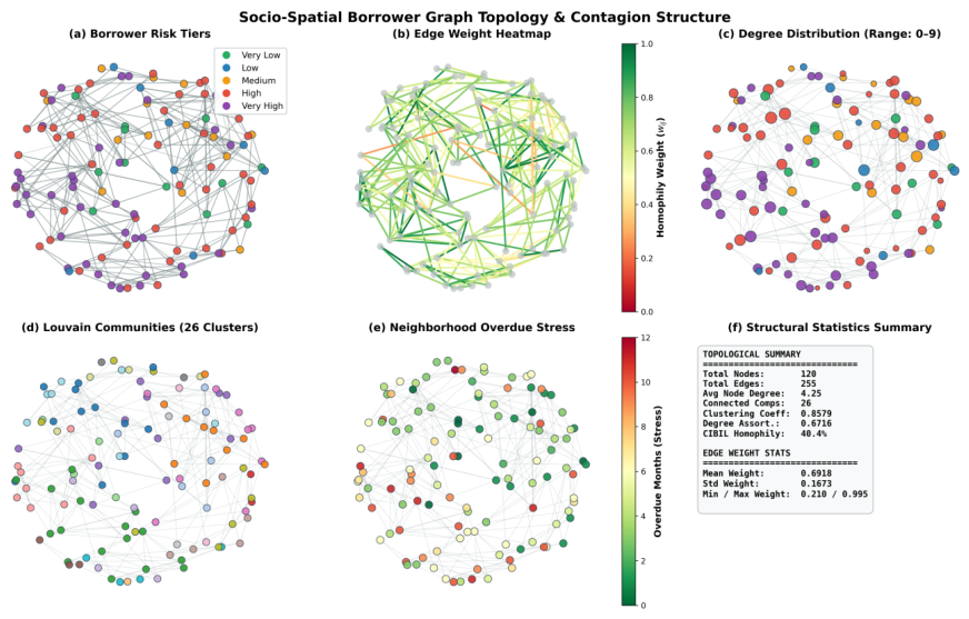
Here, is the discretized CIBIL tier (Poor, Fair, Good, Very Good, or Excellent). It is derived from an observable bureau score rather than the target label, preventing direct target-label leakage. Because the synthetic risk labels are related to CIBIL and delinquency variables, this does not establish feature independence or causal contagion. The current graph-validation artifact reports nodes and unique undirected relational edges, corresponding to mean degree . Dataset topology metrics are summarized in Table 1; architectural diagrams are illustrative and are not treated as numerical sources.
Figure 3.
Illustrative sample representation of the enhanced socio-spatial graph topology, showing Louvain community partitions and degree distributions across regional and occupational clusters. The displayed node and edge statistics describe the visualization sample, not the full 200,000-node graph.
Figure 3.
Illustrative sample representation of the enhanced socio-spatial graph topology, showing Louvain community partitions and degree distributions across regional and occupational clusters. The displayed node and edge statistics describe the visualization sample, not the full 200,000-node graph.
3.5. Structural Centrality & Homophily Metrics
For each node , three topological centrality metrics are extracted (Figure 2, Stage 3):
- Node Degree (): Direct peer count .
- PageRank (): Unweighted systemic centrality via power iteration ():
- Betweenness Centrality (): Quantifies bridging influence across regional sub-graphs:
The graph validation artifact reports a same-CIBIL-tier edge ratio of 0.9996, indicating that the current similarity-weighted construction strongly links borrowers within the same discretized credit-score tier. This is a property of the synthetic construction, not evidence of causal contagion.
3.6. Community Detection & Multi-Hop Contagion Signals
Using the Louvain modularity algorithm [21] (Figure 2, Stage 3), nodes are partitioned into dense modules maximizing modularity Q:
Community-level mean CIBIL, mean overdue months, total demand, and community size are assigned to each node; no community feature is computed from the target risk label. Sparse matrix multiplications compute walk-based multi-step stress signals for :
Together with the 9 individual features, 3 structural centrality metrics, 5 selected community and multi-hop signals, and the 16-dimensional final GAT representation, this establishes a 33-dimensional feature matrix for downstream risk classification.
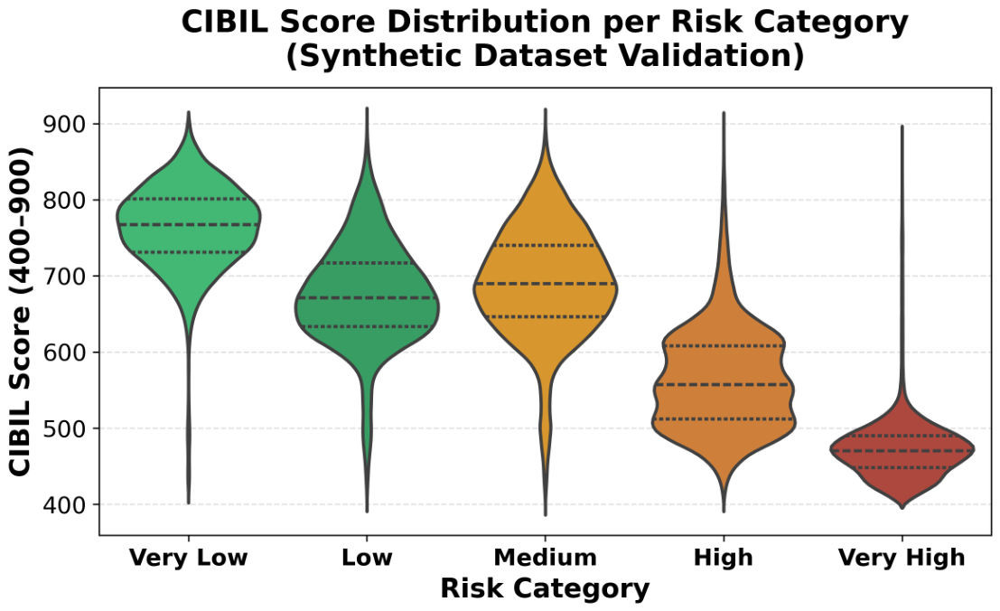
Figure 4.
CIBIL score distribution per risk tier across the 200k-node synthetic dataset
4. Socio-Spatial Graph Attention Network (GAT) Architecture
This section presents the proposed two-layer Graph Attention Network architecture and the multi-level explainability framework. Figure 5 provides an end-to-end view from raw feature input through risk classification and explainability generation.
4.1. Problem Formulation
Default risk prediction is formulated as a transductive node classification task over graph . Given node feature matrix and sparse adjacency matrix , the goal is to predict node labels corresponding to ordinal risk categories.
4.2. Graph Attention Mechanism Derivation
To aggregate neighbor features dynamically from node features and edge weights, we employ a 2-layer Graph Attention Network [11]. For node pair , attention coefficient is computed via a parameterized self-attention mechanism:
where is a weight matrix, is the attention vector, and ‖ represents vector concatenation. Normalized attention coefficients are obtained via softmax over spatial neighbors :
4.3. Multi-Head Layer Integration
To stabilize attention learning, Layer 1 employs independent attention heads concatenated together:
where denotes Batch Normalization followed by ReLU activation and 30% dropout. Layer 2 applies a single-head, edge-aware GATConv to project the 128-dimensional output into a dense 16-dimensional graph embedding , followed by a linear classifier for the five risk labels. GAT training uses only the training-node labels; graph inputs remain available for message passing without target-derived community features.
4.4. Loss Function & Optimization
The network is optimized end-to-end using Multi-Class Cross-Entropy Loss:
with weight decay and Adam optimizer ().
4.5. Benchmark Testbed Contract
The testbed is defined as a reproducible four-stage contract rather than a deployment-specific application. First, the ingestion stage accepts borrower attributes, coarse region and occupation codes, and an optional target column. Identifiers, precise addresses, and protected attributes are excluded from the model matrix. Second, the graph stage constructs the socio-spatial edge list, computes structural and multi-hop features, and exports the graph-validation record. Third, the evaluation stage consumes a fixed seed, stratified split, and named feature configuration to produce predictions, metrics, SHAP values, and attention summaries. Fourth, the artifact stage writes machine-readable CSV/JSON outputs that can be independently checked against the paper tables.
The contract exposes three benchmark tasks: (i) node-risk classification using individual features alone or with graph features, (ii) relational attribution separating individual, structural, multi-hop, and GAT-embedding contributions, and (iii) scale measurement over increasing node counts. This separation allows a baseline model to be evaluated without the GAT representation and allows the graph representation to be audited independently of the downstream classifier.
The protocol applies three leakage controls. Labels are used only in the training-node loss and evaluation target; community and neighborhood features are computed from observable borrower attributes and pre-target delinquency fields; and all scalers and classifiers are fitted on the training partition before test evaluation. The released seed, split rule, feature lists, and output schema therefore define a repeatable testbed interface rather than a single irreproducible experiment.
5. Experimental Evaluation & Comprehensive Ablation Study
5.1. Experimental Protocol & Hyperparameters
Experiments are executed on 50,000 sampled borrower nodes using an 80/20 train/test split. This evaluation uses one quarter of the 200,000-node artifact, providing a reproducible memory-bounded protocol. To evaluate and , we compare three tabular classifiers with the full graph-feature model:
- 1.
- Logistic Regression: Linear baseline on individual tabular features.
- 2.
- Random Forest (Baseline): Tree ensemble baseline on individual tabular features (9 features).
- 3.
- XGBoost / Gradient Boosting: Gradient-boosted tree baseline on individual tabular features (9 features); the current implementation uses scikit-learn GradientBoostingClassifier.
- 4.
- Full Graph Model (Ours): Random Forest classifier trained on concatenated individual features, structural centrality, multi-hop stress signals, and GAT embeddings (33 features).
5.2. Quantitative Performance & Ablation Results
As detailed in Table 3 and Figure 6, the full graph-feature model achieves the highest accuracy (79.67%) and Macro-F1 (0.6743), improving accuracy by 0.78 percentage points over the Random Forest baseline. XGBoost / Gradient Boosting has slightly higher ROC-AUC (0.9479), showing that graph features improve the selected classification metrics but do not dominate every metric. The GCN- and GraphSAGE-labelled rows are feature-subset Random Forest proxies, not separately trained neural GCN or GraphSAGE models.
Answering & : In the current comparison, adding the full graph representation increases accuracy from 78.89% to 79.67% and Macro-F1 from 0.6655 to 0.6743. This is an observed benchmark improvement, not evidence of universal superiority or causal contagion. The current run reports feature-subset proxies rather than direct neural GCN or GraphSAGE comparisons.
Scalability: The measured 100-tree Random Forest fitting times on the 17-feature input were 0.755, 2.775, 7.249, 15.170, and 31.808 seconds at 5,000, 20,000, 50,000, 100,000, and 200,000 nodes, respectively, using one worker and seed 42. These downstream-classifier measurements provide an empirical scaling baseline; they do not claim end-to-end GAT training scalability.
5.3. Error Analysis Scope
The current evaluation artifacts report aggregate classification metrics and do not provide a class-level confusion analysis for the graph classifier. The following error interpretations are therefore outside the validated result set and are not claimed here.
- Class-specific error rates and confusion patterns require a separate reported evaluation.
5.4. Selected Configuration
The reported graph representation uses four first-layer attention heads, 30% dropout, a 16-dimensional second-layer embedding, weight decay , and learning rate . Comparative hyperparameter-sweep results are not included in the current artifacts; these values define the evaluated configuration rather than a claim of optimality.
5.5. Reproducibility and Validation Record
The published evaluation uses the current 50,000-node sample, random seed 42, stratified 80/20 split, 100-tree Random Forest classifiers, and a 250-instance SHAP sample. The current graph-validation artifact contains 200,000 nodes and 633,217 unique undirected edges; the attention export contains 1,460,156 records. Because these two exports are not arithmetically identical, the attention count is reported separately and is not used to infer the validated unique-edge count. The dataset contains target-free community features and 16 exported GAT embedding dimensions. The repository runbook provides Windows commands for reproducing the baseline table, Graph-XAI outputs, scalability measurements, and paper figures; generated metrics must be synchronized into this manuscript before submission.
6. Multi-Level Graph Explainable AI (Graph-XAI)
To interpret model decisions (), we construct a multi-level explainability framework spanning global feature attribution and relational edge-attention analysis.
6.1. Level 1: Feature Taxonomy Disentanglement (SHAP)
Using SHAP TreeExplainer [18], we compute global feature attributions across 250 sampled test instances from the corrected downstream Random Forest. Features are categorized into four distinct taxonomies:
- 1.
- Individual Attributes: Income, age, CIBIL score, overdue months, EMI, current/total demand.
- 2.
- Multi-Hop Contagion Signals: 1-hop, 2-hop, 3-hop neighborhood stress tensors .
- 3.
- GAT Neural Embeddings: 16-dimensional dense node representations.
- 4.
- Graph Structural Centrality: Node degree, PageRank, and betweenness centrality.
As presented in Table 4, individual attributes account for 32.74% of aggregate mean absolute SHAP magnitude. The selected graph features account for the remaining 67.26%, with the largest share in this run assigned to the GAT embedding columns. This is a model-specific aggregate summary, not a regulatory threshold, per-borrower attribution, or causal measurement. Figure 7 illustrates the top 15 features.
6.2. Level 2: Edge Attention & Topological Interpretability
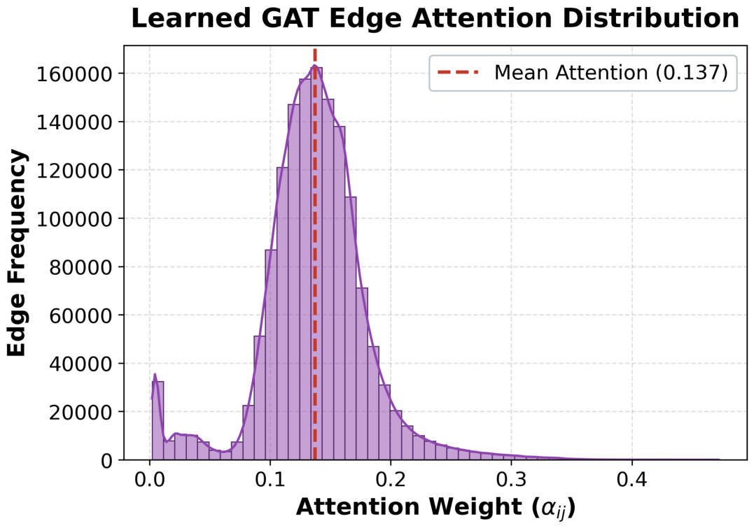
The attention export contains 1,460,156 directed layer-1 GAT attention/message records, including the layer’s message passing self-loop records. Its regenerated summary has mean 0.1370, standard deviation 0.0447, minimum 0.0021, and maximum 0.4720. These values describe learned weighting in the exported records; they do not establish that distress causes higher attention. The export count is kept separate from the graph-validation edge count because the two current files are not arithmetically identical.
Figure 8.
Learned layer-1 GAT attention-weight distribution across 1,460,156 directed message records, including self-loop records.
Figure 8.
Learned layer-1 GAT attention-weight distribution across 1,460,156 directed message records, including self-loop records.
Answering : By combining SHAP group attributions with GAT edge attention, our framework provides complementary global and relational explanations. The reported SHAP values describe aggregate feature-group importance and should not be interpreted as a per-borrower legal attribution.
7. Evaluation Scope & Limitations
The benchmark excludes identifying and protected demographic attributes from model inputs. This does not establish demographic fairness: region and occupation may still act as correlated or proxy variables, and fairness assessment requires explicit definitions and group-level evaluation [29,30]. The 67.26% selected graph attribution is an aggregate mean-absolute SHAP summary, not a regulatory threshold, per-borrower attribution, or causal measurement. Fairness, calibration, causal validation, human oversight, and production deployment remain outside the present benchmark scope.
The dataset-quality audit found zero missing cells, duplicate rows, and checked numeric-range violations across all 200,000 records. Region and occupation distributions have normalized entropies of 0.982 and 0.982, while the five-class risk distribution has entropy 0.894; the largest subgroup risk-distribution gap is 0.401 for occupation. These results support internal consistency and reproducibility, not a claim that the synthetic population is unbiased or representative; external temporal and independent-data validation remains necessary.

Table 5.
Dataset Quality and Representation Audit.
| Audit metric | Measured value |
|---|---|
| Missing-cell rate | 0.000% |
| Duplicate-row rate | 0.000% |
| Checked range violations | 0 records |
| Region distribution entropy | 0.982 |
| Occupation distribution entropy | 0.982 |
8. Conclusions
We introduced a 200,000-node socio-spatial benchmark and reproducible testbed for explainable credit-risk modeling. The benchmark makes relational structure explicit through 633,217 edges, multi-hop stress features, GAT embeddings, and machine-readable quality and scalability artifacts. On the 50,000-node evaluation sample, the full graph model achieved the strongest accuracy and Macro-F1, improving accuracy over the tabular Random Forest from 78.89% to 79.67%. SHAP assigned 67.26% of selected attribution to graph-derived features, while the scaling record extended to all 200,000 nodes. These synthetic results support controlled relational-stress experiments but do not establish causal contagion, demographic neutrality, or regulatory validity; temporal, external-data, calibration, and end-to-end resource validation remain future work.
References
- Hand, D. J. Modelling consumer credit risk. IMA J. Manag. Math. 2007, vol. 18(no. 2), 107–125. [Google Scholar]
- Lessmann, S.; Baesens, B.; Seow, C.; Thomas, L. Benchmarking state-of-the-art classification algorithms for credit scoring. Eur. J. Oper. Res. 2015, vol. 247(no. 1), 124–136. [Google Scholar] [CrossRef]
- Chen, Y.; Calabrese, R.; Martin-Barragan, B. Interpretable machine learning for imbalanced credit scoring datasets. Eur. J. Oper. Res. 2024, vol. 312(no. 1), 357–372. [Google Scholar] [CrossRef]
- Chen, H.; Zhang, H.; Li, S.; Liang, Y.; Zhang, H. Research on loan default risk prediction methods based on graph neural networks. Proc. IEEE ICCSIT, 2024. [Google Scholar]
- Eisenberg, L.; Noe, T. H. Systemic risk in financial networks. Manag. Sci. 2001, vol. 47(no. 2), 236–249. [Google Scholar] [CrossRef]
- Battiston, S.; Puliga, M.; Kaushik, R.; Tasca, P.; Caldarelli, G. DebtRank: Too central to fail? Financial networks, the FED and systemic risk. Sci. Rep. 2012, vol. 2(no. 1), 541. [Google Scholar] [CrossRef] [PubMed]
- Glasserman, P.; Young, H. P. Contagion in financial networks. J. Econ. Lit. 2016, vol. 54(no. 3), 779–831. [Google Scholar] [CrossRef]
- Zandi, S.; Korangi, K.; Óskarsdóttir, M.; Mues, C.; Bravo, C. Attention-based dynamic multilayer graph neural networks for loan default prediction. Eur. J. Oper. Res. 2024, vol. 316(no. 1), 248–261. [Google Scholar] [CrossRef]
- Scarselli, F.; Gori, M.; Tsoi, A. C.; Hagenbuchner, M.; Monfardini, G. The graph neural network model. IEEE Trans. Neural Netw. 2009, vol. 20(no. 1), 61–80. [Google Scholar] [CrossRef] [PubMed]
- Kipf, T. N.; Welling, M. Semi-supervised classification with graph convolutional networks. Proc. ICLR 2017. [Google Scholar] [CrossRef]
- Veličković, P.; Cucurull, G.; Casanova, A.; Romero, A.; Liò, P.; Bengio, Y. Graph attention networks. Proc. ICLR 2018. [Google Scholar] [CrossRef]
- Hamilton, W. L.; Ying, R.; Leskovec, J. Inductive representation learning on large graphs. Proc. NeurIPS 2017, 1024–1034. [Google Scholar]
- Guidotti, R.; Monreale, A.; Ruggieri, S.; Turini, F.; Giannotti, F.; Pedreschi, D. A survey of methods for explaining black box models. ACM Comput. Surv. 2018, vol. 51(no. 5), 1–42. [Google Scholar] [CrossRef]
- Hofmann, H. Statlog (German Credit Data). In UCI Machine Learning Repository; 1994. [Google Scholar] [CrossRef]
- Kaggle. “Give Me Some Credit: Improve on the state of the art in credit scoring,” Kaggle Competition Dataset. 2011. Available online: https://www.kaggle.com/c/GiveMeSomeCredit.
- Home Credit Group, “Home Credit Default Risk: Predict loan repayment capabilities,” Kaggle Competition Dataset. 2018. Available online: https://www.kaggle.com/c/home-credit-default-risk.
- Yeh, I.-C.; Lien, C.-h. The comparisons of data mining techniques for the predictive accuracy of probability of default of credit card clients. Expert Syst. With Appl. 2009, vol. 36(no. 2), 2473–2480. [Google Scholar] [CrossRef]
- Lundberg, S. M.; Lee, S.-I. A unified approach to interpreting model predictions. Proc. NeurIPS 2017, 4765–4774. [Google Scholar]
- Ying, R.; Bourgeois, D.; You, J.; Zitnik, M.; Leskovec, J. GNNExplainer: Generating explanations for graph neural networks. Proc. Advances in Neural Information Processing Systems (NeurIPS), 2019; pp. 9240–9251. [Google Scholar]
- Xu, L.; Skoularidou, M.; Cuesta-Infante, A.; Veeramachaneni, K. Modeling tabular data using conditional GAN. Proc. Advances in Neural Information Processing Systems (NeurIPS), 2019; pp. 7335–7345. [Google Scholar]
- Blondel, V. D.; Guillaume, J.-L.; Lambiotte, R.; Lefebvre, E. Fast unfolding of communities in large networks. J. Stat. Mech. Theory Exp. 2008, P10008. [Google Scholar] [CrossRef]
- Thomas, L. C. A survey of credit and behavioural scoring: Forecasting financial risk of lending to consumers. Int. J. Forecast. 2000, vol. 16(no. 2), 149–172. [Google Scholar] [CrossRef]
- Acemoglu, D.; Ozdaglar, A.; Tahbaz-Salehi, A. Systemic risk and stability in financial networks. Am. Econ. Rev. 2015, vol. 105(no. 2), 564–608. [Google Scholar] [CrossRef]
- Elliott, M.; Golub, B.; Jackson, M. O. Financial networks and contagion. Am. Econ. Rev. 2014, vol. 104(no. 10), 3115–3153. [Google Scholar] [CrossRef]
- Ribeiro, M. T.; Singh, S.; Guestrin, C. Why should I trust you?: Explaining the predictions of any classifier. Proc. ACM SIGKDD, 2016; pp. 1135–1144. [Google Scholar]
- Pope, P. E.; Kolouri, S.; Rostami, M.; Martin, C. E.; Hoffmann, H. Explainability methods for graph convolutional neural networks. Proc. IEEE/CVF Conference on Computer Vision and Pattern Recognition, 2019; pp. 10764–10773. [Google Scholar]
- Weber, M.; Domeniconi, G.; Chen, J.; Weidele, D. K. I.; Bellei, C.; Robinson, T.; Leiserson, C. E. Anti-money laundering in Bitcoin: Experimenting with graph convolutional networks for financial forensics. arXiv 2019, arXiv:1908.02591. [Google Scholar]
- Patki, K.; Wedge, R.; Veeramachaneni, K. The Synthetic Data Vault. Proc. IEEE International Conference on Data Science and Advanced Analytics Workshops, 2016. [Google Scholar]
- Hardt, M.; Price, E.; Srebro, N. Equality of opportunity in supervised learning. Adv. Neural Inf. Process. Syst. 2016, 3315–3323. [Google Scholar]
- Mehrabi, N.; Morstatter, F.; Saxena, N.; Lerman, K.; Galstyan, A. A survey on bias and fairness in machine learning. ACM Comput. Surv. 2021, vol. 54(no. 6), 1–35. [Google Scholar] [CrossRef]
Figure 1.
Proposed banking-data integration boundary for the offline testbed, including data ingestion, privacy filtering, and Graph-XAI processing.
Figure 1.
Proposed banking-data integration boundary for the offline testbed, including data ingestion, privacy filtering, and Graph-XAI processing.
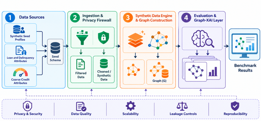
Figure 2.
Pipeline for Socio-Spatial Graph Construction, Relational Homophily Weighting, and Multi-Hop Contagion Feature Engineering.
Figure 2.
Pipeline for Socio-Spatial Graph Construction, Relational Homophily Weighting, and Multi-Hop Contagion Feature Engineering.
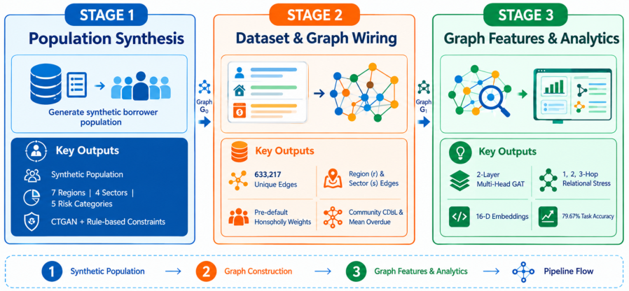
Figure 5.
End-to-End Socio-Spatial GAT Neural Architecture and Multi-Level Explainable AI (Graph-XAI) Framework.
Figure 5.
End-to-End Socio-Spatial GAT Neural Architecture and Multi-Level Explainable AI (Graph-XAI) Framework.
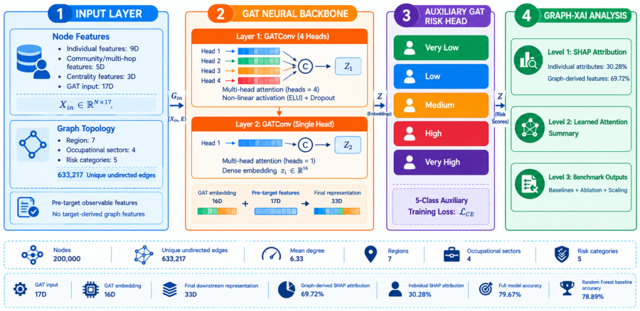
Figure 6.
Baseline and full graph-model comparison; the complete feature-subset ablation results are reported in Table 3.
Figure 6.
Baseline and full graph-model comparison; the complete feature-subset ablation results are reported in Table 3.
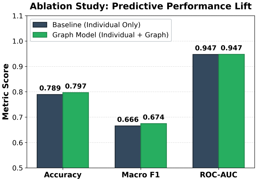
Figure 7.
Top 15 Most Influential Features for Graph Risk Classification evaluated via mean absolute SHAP values.
Figure 7.
Top 15 Most Influential Features for Graph Risk Classification evaluated via mean absolute SHAP values.
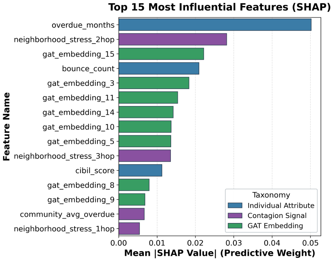
Table 1.
Comparison of Standard Credit Datasets vs. Our Socio-Spatial Relational Graph Dataset.
| Dataset | Node Count (N) | Relational Edges (M) | Spatial Topology | Occupational Homophily | Contagion Signals |
|---|---|---|---|---|---|
| UCI German Credit | 1,000 | 0 | No | No | No |
| Kaggle GiveMeSomeCredit | 150,000 | 0 | No | No | No |
| Home Credit Default Risk | 307,511 | 0 | No | No | No |
| Taiwan Credit Card | 30,000 | 0 | No | No | No |
| Our Socio-Spatial Dataset | 200,000 | 633,217 | Yes (7 Regions) | Yes (4 Sectors) | Yes (1–3 Hop Stress) |
Table 2.
Synthetic Benchmark Metadata and Quality Scope.
| Property | Verified representation |
|---|---|
| Nodes | 200,000 borrower records |
| Relational graph | 633,217 unique undirected edges |
| Socio-spatial cohorts | 7 regions × 4 occupations = 28 cohorts |
| Prediction target | Five ordinal risk categories |
| Model representation | 9 individual + 8 graph + 16 GAT features = 33 |
| Evaluation sample | 50,000 nodes; stratified 80/20 split |
| Quality audit | Missingness, duplicates, range validity, subgroup balance, and risk-distribution gaps |
| Interpretation | Structurally controlled synthetic benchmark; not a claim of real-world neutrality |
Table 3.
Tabular Baselines and Full Graph-Feature Model.
| Model Architecture | Features | Accuracy | Macro F1 | ROC-AUC (OVR) |
|---|---|---|---|---|
| Logistic Regression | 9 | 0.7728 | 0.6146 | 0.9357 |
| Random Forest (Baseline) | 9 | 0.7889 | 0.6655 | 0.9472 |
| XGBoost / Gradient Boosting | 9 | 0.7904 | 0.6528 | 0.9479 |
| Graph-feature RF (GCN subset) | 21 | 0.7479 | 0.6211 | 0.9282 |
| Graph-feature RF (GraphSAGE subset) | 8 | 0.7416 | 0.5877 | 0.9218 |
| Full Graph Model (Ours) | 33 | 0.7967 | 0.6743 | 0.9475 |
Table 4.
SHAP Feature Taxonomy Contribution Breakdown.
| Feature Taxonomy | Mean | Contribution (%) |
|---|---|---|
| Individual Attributes | 0.095255 | 32.74% |
| Multi-Hop Contagion Signals | 0.057655 | 19.82% |
| GAT Neural Embeddings | 0.137017 | 47.10% |
| Graph Structural Topology | 0.000993 | 0.34% |
| Total Systemic Graph Weight | 0.195665 | 67.26% |
Disclaimer/Publisher’s Note: The statements, opinions and data contained in all publications are solely those of the individual author(s) and contributor(s) and not of MDPI and/or the editor(s). MDPI and/or the editor(s) disclaim responsibility for any injury to people or property resulting from any ideas, methods, instructions or products referred to in the content. |
© 2026 by the authors. Licensee MDPI, Basel, Switzerland. This article is an open access article distributed under the terms and conditions of the Creative Commons Attribution (CC BY) license (http://creativecommons.org/licenses/by/4.0/).
Copyright: This open access article is published under a Creative Commons CC BY 4.0 license, which permit the free download, distribution, and reuse, provided that the author and preprint are cited in any reuse.