
Submitted:
04 September 2026
Posted:
07 September 2026
You are already at the latest version
Abstract
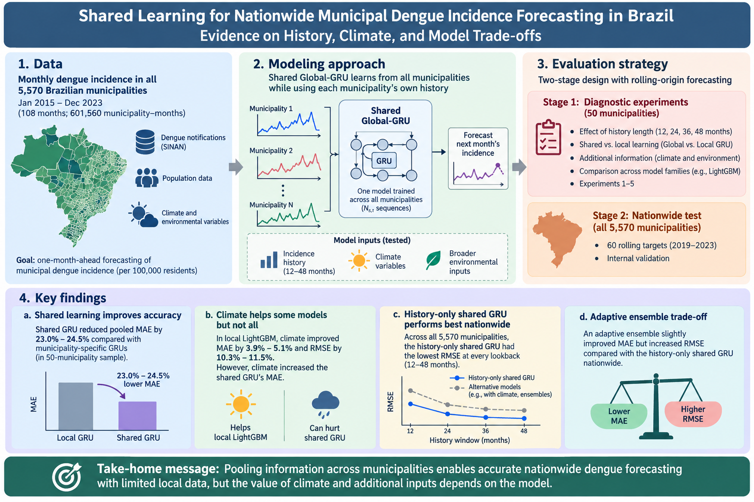
Municipality-level dengue forecasting is challenging because each time series is short. Additional predictors also do not always provide useful information. We evaluated one-month-ahead monthly incidence across all 5,570 Brazilian municipalities. The evaluation used 60 rolling targets and history windows of 12–48 months. We first used a 50-municipality diagnostic sample to test history, shared versus local learning, additional information, and neural models. We then conducted nationwide internal validation. In the diagnostic sample, the shared gated recurrent unit (GRU) reduced pooled MAE by 23.0%–24.5% compared with municipality-specific GRUs. Climate improved local LightGBM (MAE, 3.9%–5.1%; RMSE, 10.3%–11.5%). However, climate increased the shared GRU’s MAE. The predictive value of climate therefore depended on the model. Nationwide, the history-only shared GRU had the lowest RMSE at every lookback. An adaptive ensemble slightly improved MAE but increased RMSE.
Keywords:
dengue forecasting
; municipal incidence
; global forecasting models
; shared learning
; GRU
; climate covariates
; rolling-origin evaluation
; Brazil
1. Introduction
Dengue incidence changes sharply across places and months. Brazil’s 5,570 municipalities differ in epidemic history, climate, population, and surveillance. Many municipal records show long periods of low incidence followed by large peaks. Average accuracy alone does not capture this pattern. A useful model must also control large errors when incidence is high. The global surge reported in 2024 further shows the need for local forecasting at scale [1].
Municipal models face a basic data problem. Each municipality provides only a short monthly series. Flexible models and large predictor sets usually need more data. A model trained across municipalities can learn shared patterns. The same model can still use each municipality’s own history at prediction time. Climate and environmental variables may add useful information. They may also repeat existing signals, contain noise or missing values, or be poorly aligned with the forecast date.
Dengue studies have used statistical, tree-based, neural, spatial, and ensemble methods. Their scores are rarely comparable because the targets, horizons, time scales, and geographic units differ [2]. Brazilian studies have tested recent-case information, weekly continuous forecasts, models shared across groups of cities, and transfer across countries [3,4,5,6]. Pooled learning has also performed better than separate departmental models in Colombia [7]. Other work has tested climate, spatial structure, mobility, and ensembles [8,9,10,11]. Nationwide Brazilian studies have often predicted threshold events instead of continuous municipal incidence [12,13]. Global forecasting theory supports learning one parameter set across related but different series [14,15].
This study asks four questions. First, we examine how accuracy changes with the length of incidence history. Second, we test whether shared learning improves on separate Local GRUs. Third, we test whether climate and broader environmental inputs help across model families. Finally, we compare history-only designs nationwide. Experiments 1–5 address these questions in a fixed sample of 50 municipalities. Experiment 6 tests the selected models across all municipalities. The comparisons are predictive, not causal. Figure 1 shows the study sequence.
2. Data and Methods
2.1. Data, Target, and Study Stages
We analyzed monthly dengue incidence per 100,000 residents in all 5,570 Brazilian municipalities. The study period ran from January 2015 to December 2023. The data cover 108 months and 601,560 municipality–months. Dengue notifications came from SINAN. Official statistics provided population denominators and the list of municipalities [16,17]. We did not retain exact extraction dates, denominator handling, environmental data versions, or panel-building code. Supplementary Section S8 lists these gaps. Reporting delays and later revisions are also sources of measurement error [18].
For each target month s, the model used information available through the previous month, . For municipality m and history length , the incidence input and final forecast were
where is the incidence-scale raw forecast. We evaluated 60 targets from January 2019 through December 2023.
Stage 1 used a fixed diagnostic sample of 50 municipalities. We chose 10 equally spaced positions from the 2015–2018 mean-incidence ranking in each macroregion after limiting the data to complete panels and resolving ties in code. The sample covered different regions and levels of past incidence, but it was not a probability sample. Nationwide internal validation used all 5,570 municipalities, including the Stage 1 locations, over the same target months.
2.2. Rolling-Origin Neural Samples and Validation
For each target month s, the preprocessing and model-fitting steps used only data available at the forecast date. We define as January 2015. We used the following target sets:
Each fitting target r used . We filled positions before January 2015 with the municipality’s mean from the fitting period. The value of L controls the input length, not the number of fitting targets. The final 12 available targets selected the checkpoint without updating the parameters (Figure 2).
At each origin, municipality-specific scaling used original fitting observations through :

Table 1.
Dataset and forecasting protocol.
| Component | Definition used in the study |
|---|---|
| Study population | All 5,570 Brazilian municipalities; 601,560 municipality–month records. |
| Stage-1 sample | Fixed diagnostic sample of 50 municipalities, with 10 selected from each of the five Brazilian macroregions. |
| Nationwide sample | All 5,570 municipalities, used in Experiment 6 and the nationwide L12 TiDE-style comparison. |
| Observation period | January 2015–December 2023 (108 monthly observations per municipality). |
| Evaluation period | January 2019–December 2023, corresponding to 60 rolling target months; each forecast origin is the preceding month. |
| Forecast target | Monthly municipal dengue incidence rate (cases per 100,000 population). |
| Forecast horizon | One month ahead: information available through forecast origin t is used to predict the target month . |
| Lookback windows | , , , and (12, 24, 36, and 48 months, respectively). Nationwide verification of the TiDE-style dense comparator was performed at only. |
| Evaluation design | Rolling-origin evaluation. Models and preprocessing were rebuilt at each origin using only forecast-available data; the target observation was used only for scoring. Neural models used origin-specific validation and scaling. |
| Information sets | History-only, history plus climate, and history plus climate and broader environmental features, depending on the experiment. Climate inputs in corrected Experiment 4 are aligned to the forecast-origin information set. |
| Primary metrics | Mean absolute error (MAE) and root mean squared error (RMSE), computed in incidence units after inverse transformation and clipping negative forecasts to zero. |
| Secondary metric | Symmetric mean absolute percentage error (sMAPE); interpreted cautiously because the data contain zero and near-zero incidence values. |
| Prediction constraint | If is a raw incidence-scale forecast, the scored forecast is . Transformed or standardized predictions are first returned to incidence units; LightGBM predicts incidence directly. |
| Aggregation convention | Pooled metrics weight every municipality–target row equally. Municipality win counts give every municipality one vote. Multi-seed tables average metrics computed separately for each training run. |
Notes: Stage 1 covers all macroregions but is not a probability sample. Complete-panel eligibility was determined retrospectively; all forecasts still used origin-available inputs only. Comparisons are predictive, not causal.
If the population standard deviation (ddof = 0) was zero, we replaced it with one. For specification h, we define . The set contains one municipality for a Local model. The same set contains all available municipalities for a Global model. The neural networks minimized MSE on the standardized scale:
Here, is the input for a given model specification. The function represents the network. We used the checkpoint with the lowest validation loss. We did not refit the network on the combined blocks. Each target–lookback–model–seed combination started from a new initialization.
G0 was a one-layer, 16-unit GRU that used history only. G1 added 48 climate channels. L0 was the matching LSTM. G0 and G1 had 929 and 3,233 parameters, so the comparison was not matched for model size. Supplementary Section S2 gives the optimizer, early stopping rule, seeds, dropout, and padding.
We define as the mean fitting loss for municipality m. We define as its sequence count. Each Local model minimizes a separate loss. The Global model shares one parameter set:
Here, Global means shared parameters, not combined incidence. The balanced panel gave each municipality the same number of sequences at a target. We did not use municipality identifiers or geographic weights. Each forecast kept the history and scale of its municipality (Figure 3).
2.3. Features and Family-Specific Preprocessing
All predictors ended by . The climate block used 16 measures of temperature, precipitation, humidity, pressure, and thermal range. Each measure had a one-month lag and trailing means of 3 and 6 months, which gave 48 variables (Supplementary Table S1). We aggregated weekly fields to months. Supplementary Section S8 lists the climate data sources and the remaining gaps in reproducibility.
Corrected G1 paired incidence with rows of the climate matrix after lagging. The final row index is s, but the raw climate data end at . We standardized each channel with finite pooled fitting cells. We safely replaced invalid scales and set missing standardized values to zero. G0 and G1 used the same targets, splits, and optimization in all other respects.
Experiment 3A modeled and converted predictions back with . M0 used history. M1 added lagged temperature, humidity, and rainy days. M2 added eight environmental variables. Scalers used the current fitting window. If a required input was not finite, the forecast was marked unavailable. Local LightGBM predicted incidence directly and filled missing values with the fitting mean without scaling. Separate fixed models compared history, climate, and broader environmental inputs. Supplementary Sections S4–S5 give the variable names, stability rules, model settings, and limits of the recovered LightGBM record [19].
2.4. Models, Experiments, and Ensembles
Seasonal Naive used . Auto-SARIMA selected one fixed order for each municipality and lookback from a small set of candidate models. We fitted the candidates to the L months ending in December 2018. A fit was eligible if it converged, gave a finite forecast, and had finite
where p is the number of fitted parameters and n is the fit length. At each origin, we refitted the selected order to the last L observations. We first used constrained fitting and then relaxed fitting. If both attempts failed, Experiment 1 used Seasonal Naive, but Experiment 3A marked the forecast unavailable. Supplementary Section S4 gives the candidate orders and fallback rules.
Table 2 shows the experiment sequence. Experiment 2 compared Local and Global GRUs. Experiment 3 tested additional information. Experiment 4 compared G0 and G1 after we corrected the climate alignment. Experiment 5 compared G0, L0, and a history-only Transformer. Experiment 6 tested G0, L0, and two ensembles nationwide. An L12 sensitivity analysis used a TiDE-style dense model with 5,057 parameters. This comparator was not the full published TiDE architecture [20,21,22,23]. The fixed models also had different numbers of parameters.
We report only the corrected Experiment 4 results. Failed forecasts in Experiment 3A stayed unavailable. For nationwide results, we calculated each metric for each seed and then averaged the metrics. Experiment 6 reused 2019–2023 outcomes from earlier stages, so it is broad internal validation, not a frozen future test. Supplementary Section S8 lists the limits of the execution records.
The equal ensemble averaged G0 and L0. The past-origin inverse-MAE ensemble is called the adaptive ensemble below. This ensemble gave more weight to the model with lower past MAE for the same municipality. We omit the seed and lookback indices. For each target , the adaptive ensemble used the following rule:
The weights were for the first target. We also used when past MAEs were unavailable or added to zero. The rule did not use current or future outcomes, but it assumed that earlier outcomes were available without reporting delay.
2.5. Metrics and How Results Were Aggregated
After inverse transformation and zero-clipping, we define for scored row i. We calculated the following metrics:
MAE measures the average absolute error. RMSE gives more weight to large errors. Both metrics use incidence per 100,000 and served as the main outcomes. MSE uses squared units. sMAPE ranges from 0% to 200%. We treated sMAPE as a secondary metric. Every zero-versus-positive pair receives a score of 200%, regardless of the error size [24]. The metrics can therefore rank models differently [25].
The nationwide pooled metrics gave equal weight to all rows within seed b. For each run-specific metric , the tables report
Here, is the mean of three complete-run metrics. Repeated seeds are not new epidemiological outcomes. For municipality wins, we first calculated a 60-target metric for each municipality and averaged it across seeds. Each municipality then had one vote. Macroregion summaries used unweighted means across municipalities. Intensity analyses stacked 1,002,600 forecasts but contained 334,200 distinct outcomes.
Either Experiment 3A model could fail. We therefore based each comparison on . This set contains the rows with finite forecasts from both models:
Positive means that adding climate (M1) improved the metric. We reported coverage separately and did not recode or penalize failures.
For one row set, up to rounding. We define for run b. The following relation holds after averaging across runs:
The difference is the population variance of RMSE across runs. Mean MSE therefore usually differs from squared mean RMSE. We calculated G0/L0 residual correlations as centered Pearson correlations within each seed–lookback pair.
Incidence groups used the linearly interpolated 2015–2018 municipal 90th percentile, . The groups were zero, positive non-high (), and high (). The groups use the observed target, so the high-incidence analysis is retrospective and is not an outbreak forecast. Supplementary Table S2 lists the notation.
3. Results
3.1. History and Shared Learning
Incidence history supported useful predictions, but the model ranking changed by metric. Compared with Seasonal Naive, Auto-SARIMA reduced MAE by 12.4%–34.2% and RMSE by 16.7%–22.4% at L24–L48. Auto-SARIMA increased RMSE at L12 and increased sMAPE at every lookback. The model used 97, 18, 3, and 1 fallback forecasts at L12–L48 (Table 3).
Shared training improved Stage 1 performance. Across L12–L48, the Global GRU reduced pooled MAE by 23.0%–24.5% and RMSE by 16.1%–18.7%. The Global GRU also lowered municipality-level MAE in 38–39 of 50 locations (Table 4). This comparison covers only the 50-municipality diagnostic sample. We did not test Local GRUs nationwide.
3.2. Additional Information
The climate effects in the SARIMA family changed with lookback. On common finite rows, M1 increased L12 MAE by 23.2% and RMSE by 43.1%. At L24–L48, M1 reduced MAE by 1.0%–8.6% and RMSE by 2.3%–8.2%. The model also improved sMAPE at every lookback. The common-valid counts were 2,903, 2,916, 2,883, and 2,939 (Table 5, Panel A).
M2 did not support a performance comparison. Of 12,000 forecasts, 3,549 failed or were unavailable. Another 125 forecasts were labeled explosive. The combined metrics were not finite. We therefore report instability, not accuracy, for M2 (Supplementary Section S4).
Climate improved local LightGBM at every lookback. MAE fell by 3.9%–5.1%, and RMSE fell by 10.3%–11.5%. Adding the broader environmental block increased MAE by 1.2%–2.8% and RMSE by 1.3%–1.9%. None of the planned ablations improved every metric at every lookback (Figure 4Figure 5).
The shared GRU showed a different pattern. Compared with G0, G1 increased MAE by 2.1%–4.3%, changed RMSE by only % to +0.2%, and reduced sMAPE by about 19% (Table 6). G1 lowered municipality-level MAE in 27–29 of 50 locations, but its pooled MAE was worse (Figure 6Figure 7). These results are descriptive because the comparison used only two seeds and had no matching significance test.
3.3. Neural Model Comparisons and Nationwide Internal Validation
In Stage 1, G0 had the lowest RMSE at every lookback. Its RMSE was 0.8%–1.1% below L0, and T0 was 6.4%–19.2% above G0. L0 had the lowest MAE at three lookbacks. T0 had the lowest sMAPE, but its accuracy and stability became worse with longer histories (Table 7). The models had different numbers of parameters, so this is not a test of architecture alone.
Nationwide, every run–model–lookback combination produced 334,200 finite forecasts. G0 had the lowest RMSE at every lookback. Its RMSE was 0.5%–1.7% below L0. The adaptive ensemble had the lowest MAE. Its MAE was 0.2%–1.6% below G0. However, the adaptive ensemble increased RMSE by up to 0.7%. Equal weighting showed the same pattern. G0/L0 residual correlations were 0.9882–0.9952. These high correlations show that their errors moved almost together (Table 8).
Among 334,200 distinct targets, 52,168 were high-incidence, 75,190 positive non-high, and 206,842 zero. G0 had lower high-incidence MAE and RMSE than the adaptive ensemble at every lookback (Figure 8; Supplementary Table S4).
At L12, TiDE-style reduced overall sMAPE by 4.2% compared with G0. However, TiDE-style increased MAE by 0.5% and RMSE by 2.1%. TiDE-style improved MAE and RMSE for positive non-high and zero targets. The model made all three metrics worse in high-incidence months. TiDE-style also produced more raw negative forecasts (13.5% compared with 6.3%; Table 9; Figure 9). This L12-only result does not provide a general ranking of the architectures.
Supplementary Figure S1 shows five example L12 trajectories. The case-selection and seed details are unknown, so these examples cannot support claims about typical or overall performance.
We selected G0 for future validation for several reasons. The model had the lowest nationwide RMSE and stronger results in high-incidence months. The model also provided complete coverage, low variation across runs, and a one-model design. L12 gave the lowest retrospective overall and high-incidence MAE and RMSE for G0. However, we did not choose this lookback in advance. A frozen future period must confirm the choice.
4. Discussion
4.1. What the Experiments Show
Shared training performed better than separate Local GRUs in Stage 1. The climate results were mixed. Climate improved every local LightGBM setting, gave mixed gains for SARIMAX, and raised the shared GRU’s pooled MAE. Nationwide, the adaptive ensemble had the lowest MAE, but G0 gave lower RMSE and lower errors in high-incidence months with one model. The model choice depends on which error matters in practice.
The scope of each result is important. Experiments 1–5 are diagnostic tests from 50 fixed municipalities. Experiment 6 covers all municipalities, but it reuses the 2019–2023 period used for earlier choices. Experiment 6 therefore remains internal validation. The Global-versus-Local result comes only from Stage 1. We did not fit Local GRUs nationwide.
4.2. Why a Shared Model Can Help—And When It May Not
A Local GRU estimates hundreds of parameters from one short series. G0 estimates one set of parameters from many municipal sequences and keeps the local history for prediction. Shared learning can capture seasonal or epidemic patterns that repeat across places and can make estimation more stable [14,15]. This matches evidence on pooled learning from Colombia and the strong value of recent cases in Brazilian cities [3,7].
This experiment cannot show why shared learning helped. Transfer, shrinkage, more stable training, and similarity across municipalities may all play a role. Local GRUs still had lower MAE in 11–12 Stage 1 municipalities at each lookback. Future work could test fixed regional groups or small local adaptation layers [5,6].
The nationwide G0/L0 result addresses a different question because both models share parameters. Under these fixed settings, G0 had lower RMSE. This result does not show that GRUs are always better than LSTMs. Longer histories were not always better. Auto-SARIMA improved after L12, but the improvement was not steady. Errors from the recurrent models changed little. T0 became worse as its fixed window grew. The lookback length is a model choice, not a measure of dengue’s biological memory.
4.3. Why Climate Helps Some Models but Not Others
One result was unexpected. The same 48-variable climate block improved local LightGBM at all four lookbacks. However, the block increased pooled MAE for the shared GRU. SARIMAX improved only at L24–L48 on common-valid rows. The effects also differed across municipalities. Past studies have also found that climate gains change by city, spatial unit, forecast horizon, and target [8,10,11,12].
Recent incidence may already contain part of the information about transmission. Monthly data can hide shorter climate lags. Weather measured for a whole municipality may also be a poor match for local exposure. Missing data and reporting delays add more mismatch [18,26]. These are possible explanations, but the experiments did not test the causes directly.
M2 shows only that the model was numerically unstable. This result does not show that its environmental variables lack biological or predictive value. The inverse transform can make errors on the fitted scale much larger. The following approximation illustrates this effect for :
A large u therefore makes a small change much larger. This pattern is consistent with the explosive M2 forecasts. However, the approximation does not identify their cause.
The LightGBM ablations show another limit. A few better results across many groups, metrics, and windows do not show a reliable gain. The value of extra environmental information changed with its representation, the model, the metric, and the location. These prediction tests do not measure causal climate effects.
4.4. What the Metrics and Ensembles Mean in Practice
MAE measures a typical absolute error. RMSE gives more weight to large errors. sMAPE treats every zero-versus-positive pair as 200% [24]. T0 and TiDE-style could therefore improve sMAPE while making incidence-scale errors worse. TiDE-style also produced more negative raw forecasts. Zero-clipping then created more exact zeros and improved its scores for zero targets.
The ensemble reduced MAE but did not reduce RMSE. For component errors and , a constant G0 weight w gives
The cross-term depends on correlation, error size, and bias. The cross-moment is . Our weights changed by municipality, target, lookback, and seed. We therefore calculated the ensemble errors directly. Residual correlations of 0.9882–0.9952 show that the component errors moved together. This pattern helps explain why RMSE did not improve. The small MAE gain must be compared with the cost of keeping a second model.
The high-incidence analysis tests performance on large errors, but the analysis is retrospective because the groups use the observed target. G0’s advantage supports model selection based on RMSE. The advantage does not support claims about outbreak sensitivity, lead time, or false alerts. An operational test must set thresholds in advance and use timely data. The test must also score missed and false alerts and measure uncertainty [27,28].
If MAE is the main goal, the adaptive ensemble is the better choice. If overall sMAPE or zero-target error is the main goal, TiDE-style may be better at L12. We gave more weight to control of large errors, performance in high-incidence months, nationwide coverage, and the simplicity of one model. With these priorities, G0 is the candidate for future validation, not for deployment.
History-only G0 does not depend on external variables that may arrive at different times across the country. However, the model forecasts recorded notifications. These data reflect care seeking, diagnosis, and reporting as well as transmission. We did not test resource allocation, health outcomes, or equity. Any operational use should track data completeness and errors across groups. Local judgment should remain part of the process.
4.5. Limitations and the Next Test
The main limitation is temporal. We did not test the models on an untouched future period. Stage 1 was fixed but not random. The nationwide analysis reused the 2019–2023 period used to choose models. Notifications can also be delayed, revised, missed, or classified in different ways [18,29]. We forecast recorded incidence, not unobserved infections.
The seed schedule used in Experiment 2 was not kept. The neural models had different sizes. Corrected G0/G1 used two seeds, and no saved significance test was available. Experiment 3A uses common-valid rows, M2 was unstable, and TiDE-style was tested only at L12. We also could not recover the selection rule or seed for the five example trajectories.
The study can be reproduced only in part, not byte for byte. We did not keep package versions, hardware details, or the rainy-day threshold. We also did not keep some LightGBM construction details or the raw nationwide finalizer. The saved predictions and result summaries can still be checked. However, the missing records prevent an exact rerun.
If we ran the study again, we would keep a later period untouched from the start. We would also fix the data versions, release times, lookback, alert thresholds, and main loss before choosing a model. A future test should check probability calibration and interval coverage. The test should compare shared, hierarchical, and region-adaptive models under the same controls against data leakage.
5. Conclusions
Shared training reduced Stage 1 pooled MAE by 23.0%–24.5%. The value of climate and broader environmental inputs changed with the model and metric. Nationwide, the adaptive ensemble slightly improved MAE, but history-only G0 gave lower RMSE and lower errors in high-incidence months with one model. We recommend G0 for a future-period test planned in advance, not as a universal model or a model ready for use.
References
- World Health Organization. Dengue. Fact sheet, 2025. WHO Fact.-Sheet Rec. accessed. 2025. (accessed on Aug. 28 2026). [Google Scholar] [CrossRef]
- Leung, X.Y.; Islam, R.M.; Adhami, M.; Ilic, D.; McDonald, L.; Palawaththa, S.; Diug, B.; Munshi, S.U.; Karim, M.N. A systematic review of dengue outbreak prediction models: Current scenario and future directions. PLoS Neglected Trop. Dis. 2023, 17, e0010631. [Google Scholar] [CrossRef] [PubMed]
- Roster, K.; Connaughton, C.; Rodrigues, F.A. Machine-Learning-Based Forecasting of Dengue Fever in Brazilian Cities Using Epidemiologic and Meteorological Variables. Am. J. Epidemiol. 2022, 191, 1803–1812. [Google Scholar] [CrossRef] [PubMed]
- Mussumeci, E.; Coelho, F.C. Large-scale multivariate forecasting models for Dengue— LSTM versus random forest regression. Spat. Spatio-Temporal Epidemiol. 2020, 35, 100372. [Google Scholar] [CrossRef] [PubMed]
- de Freitas Saldanha, R.; Ribeiro, V.; Pena, E.H.M.; Pedroso, M.; Akbarinia, R.; Valduriez, P.; Porto, F. Subset Models for Multivariate Time Series Forecast. In Proceedings of the 2024 IEEE 40th International Conference on Data Engineering Workshops (ICDEW), Utrecht, Netherlands, 2024; pp. 86–90. [Google Scholar] [CrossRef]
- Kristjanpoller, W.; Fernandes, L.H.S.; Jale, J.S.; Silva, M.A.R.; Tabak, B.M. From global to local: A transfer learning framework for municipal dengue prediction in Brazil. Physica A Stat. Mech. Its Appl. 2026, 688, 131375. [Google Scholar] [CrossRef]
- Zhao, N.; Charland, K.; Carabali, M.; Nsoesie, E.O.; Maheu-Giroux, M.; Rees, E.; Yuan, M.; Garcia Balaguera, C.; Jaramillo Ramirez, G.; Zinszer, K. Machine learning and dengue forecasting: Comparing random forests and artificial neural networks for predicting dengue burden at national and sub-national scales in Colombia. PLoS Neglected Trop. Dis. 2020, 14, e0008056. [Google Scholar] [CrossRef] [PubMed]
- Chen, X.; Moraga, P. Forecasting dengue across Brazil with LSTM neural networks and SHAP-driven lagged climate and spatial effects. BMC Public Health 2025, 25, 973. [Google Scholar] [CrossRef] [PubMed]
- Chen, X.; Moraga, P. Dengue forecasting and outbreak detection in Brazil using LSTM: Integrating human mobility and climate factors. Infect. Dis. Model. 2026, 11, 338–354. [Google Scholar] [CrossRef] [PubMed]
- Sebastianelli, A.; Spiller, D.; Carmo, R.; Wheeler, J.; Nowakowski, A.; Jacobson, L.V.; Kim, D.; Barlevi, H.; El Raiss Cordero, Z.; Colón-González, F.J.; et al. A reproducible ensemble machine learning approach to forecast dengue outbreaks. Sci. Rep. 2024, 14, 3807. [Google Scholar] [CrossRef] [PubMed]
- da Silva, S.T.; Gabrick, E.C.; Protachevicz, P.R.; Iarosz, K.C.; Caldas, I.L.; Batista, A.M.; Kurths, J. When climate variables improve the dengue forecasting: A machine learning approach. Eur. Phys. J. Spec. Top. 2025, 234, 555–569. [Google Scholar] [CrossRef]
- Danko, D.C.; Vörösmarty, C.; Cak, A.; Corsi, F.; Patel, S.; Papciak, J.; Wells, H.; Albanese, A.; Mason, C.E.; Maciel-de Freitas, R.; et al. Forecasting Dengue Fever in Brazil Using Multimodal Data, Including Climate Data. bioRxiv 2024. Prepr. Version 1 2024. [Google Scholar] [CrossRef]
- Villela, D.A.M. Predicting high dengue incidence in municipalities of Brazil using path signatures. Sci. Rep. 2025, 15, 26733. [Google Scholar] [CrossRef] [PubMed]
- Montero-Manso, P.; Hyndman, R.J. Principles and algorithms for forecasting groups of time series: Locality and globality. Int. J. Forecast. 2021, 37, 1632–1653. [Google Scholar] [CrossRef]
- Bandara, K.; Bergmeir, C.; Smyl, S. Forecasting across time series databases using recurrent neural networks on groups of similar series: A clustering approach. Expert Syst. With Appl. 2020, 140, 112896. [Google Scholar] [CrossRef]
- Ministério da Saúde; Brazil. Sinan/Dengue. Portal de Dados Abertos do SUS, 2026; accessed; SINAN open-data record, Aug 2026; (accessed on Aug. 28 2026). [Google Scholar]
- Instituto Brasileiro de Geografia e Estatística. Estimates of resident population for municipalities and federation units. Population Estimates. IBGE population-estimates record. Accessed. n.d. (accessed on Aug. 28 2026).
- Bastos, L.S.; Economou, T.; Gomes, M.F.C.; Villela, D.A.M.; Coelho, F.C.; Cruz, O.G.; Stoner, O.; Bailey, T.; Codeço, C.T. A modelling approach for correcting reporting delays in disease surveillance data. Stat. Med. 2019, 38, 4363–4377. [Google Scholar] [CrossRef] [PubMed]
- Ke, G.; Meng, Q.; Finley, T.; Wang, T.; Chen, W.; Ma, W.; Ye, Q.; Liu, T.Y. LightGBM: A highly efficient gradient boosting decision tree. Proc. Adv. Neural Inf. Process. Syst. Available. 2017, Vol. 30, 3146–3154. [Google Scholar]
- Cho, K.; van Merriënboer, B.; Gulcehre, C.; Bahdanau, D.; Bougares, F.; Schwenk, H.; Bengio, Y. Learning Phrase Representations using RNN Encoder–Decoder for Statistical Machine Translation. In Proceedings of the Proceedings of the 2014 Conference on Empirical Methods in Natural Language Processing (EMNLP), Doha, Qatar, 2014; pp. 1724–1734. [Google Scholar] [CrossRef]
- Hochreiter, S.; Schmidhuber, J. Long Short-Term Memory. Neural Comput. 1997, 9, 1735–1780. [Google Scholar] [CrossRef] [PubMed]
- Vaswani, A.; Shazeer, N.; Parmar, N.; Uszkoreit, J.; Jones, L.; Gomez, A.N.; Kaiser; Polosukhin, I. Attention Is All You Need. In Proceedings of the Advances in Neural Information Processing Systems; Available; Curran Associates, Inc.; NeurIPS record, 2017; Vol. 30, pp. 5998–6008. [Google Scholar]
- Das, A.; Kong, W.; Leach, A.; Mathur, S.K.; Sen, R.; Yu, R. Long-term Forecasting with TiDE: Time-series Dense Encoder. In Transactions on Machine Learning Research; Available; OpenReview record, 2023. [Google Scholar]
- Hyndman, R.J.; Koehler, A.B. Another look at measures of forecast accuracy. Int. J. Forecast. 2006, 22, 679–688. [Google Scholar] [CrossRef]
- Gneiting, T. Making and Evaluating Point Forecasts. J. Am. Stat. Assoc. 2011, 106, 746–762. [Google Scholar] [CrossRef]
- Sylvestre, E.; Joachim, C.; Cécilia-Joseph, E.; Bouzillé, G.; Campillo-Gimenez, B.; Cuggia, M.; Cabié, A. Data-driven methods for dengue prediction and surveillance using real-world and Big Data: A systematic review. PLoS Neglected Trop. Dis. 2022, 16, e0010056. [Google Scholar] [CrossRef] [PubMed]
- Lowe, R.; Coelho, C.A.S.; Barcellos, C.; Carvalho, M.S.; De Castro Catão, R.; Coelho, G.E.; Ramalho, W.M.; Bailey, T.C.; Stephenson, D.B.; Rodó, X. Evaluating probabilistic dengue risk forecasts from a prototype early warning system for Brazil. eLife 2016, 5, e11285. [Google Scholar] [CrossRef] [PubMed]
- Araujo, E.C.; Carvalho, L.M.; Ganem, F.; Vacaro, L.B.; Bastos, L.S.; Freitas, L.P.; de Almeida, I.F.; Bastos, M.; Alencar, R.; Bianchi, L.; et al. Leveraging probabilistic forecasts for dengue preparedness and control: The 2024 Dengue Forecasting Sprint in Brazil. Proc. Natl. Acad. Sci. 2026, 123, e2508989123. [Google Scholar] [CrossRef] [PubMed]
- Silva, M.M.O.; Rodrigues, M.S.; Paploski, I.A.D.; Kikuti, M.; Kasper, A.M.; Cruz, J.S.; Queiroz, T.L.; Tavares, A.S.; Santana, P.M.; Araújo, J.M.G.; et al. Accuracy of dengue reporting by national surveillance system, Brazil. Emerg. Infect. Dis. 2016, 22, 336–339. [Google Scholar] [CrossRef] [PubMed]
Figure 1.
The study pipeline has two evaluation stages. Stage 1 supports diagnostic comparisons. The nationwide stage remains internal validation because it reuses the 2019–2023 evaluation period.
Figure 1.
The study pipeline has two evaluation stages. Stage 1 supports diagnostic comparisons. The nationwide stage remains internal validation because it reuses the 2019–2023 evaluation period.

Figure 2.
The rolling-origin evaluation follows three steps for target s. The model fits its parameters, selects a checkpoint using the preceding 12 targets, and reveals only for scoring.
Figure 2.
The rolling-origin evaluation follows three steps for target s. The model fits its parameters, selects a checkpoint using the preceding 12 targets, and reveals only for scoring.

Figure 3.
The figure shows the shared Global-GRU architecture. The original schematic uses , , and for the origin-specific scale. One GRU learns from sequences. The model converts forecasts back to municipal incidence units and clips negative values at zero.
Figure 3.
The figure shows the shared Global-GRU architecture. The original schematic uses , , and for the origin-specific scale. One GRU learns from sequences. The model converts forecasts back to municipal incidence units and clips negative values at zero.
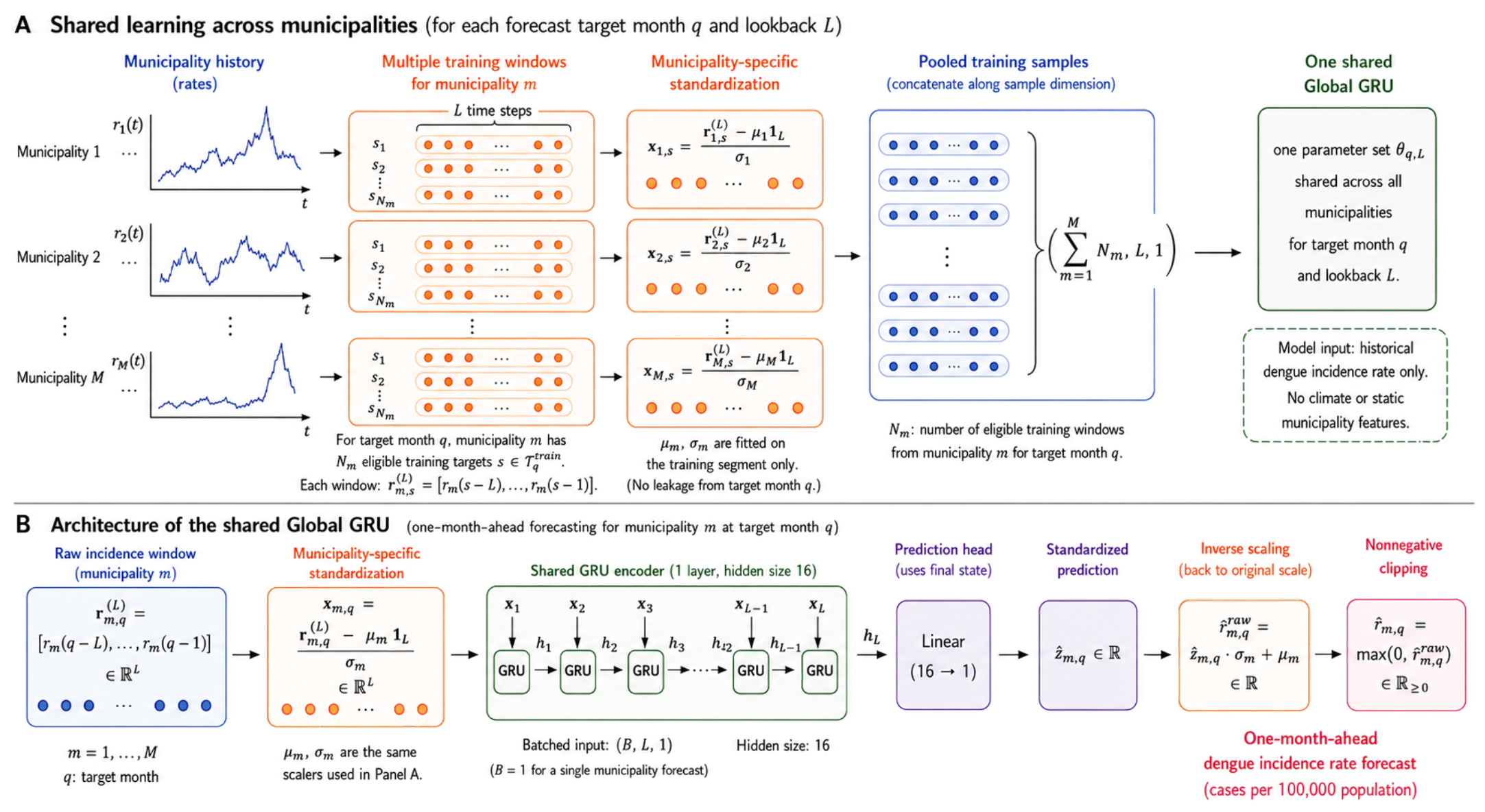
Figure 4.
The figure compares information sets within the Stage 1 local-LightGBM family ( per condition and lookback). Lower values indicate better performance.
Figure 4.
The figure compares information sets within the Stage 1 local-LightGBM family ( per condition and lookback). Lower values indicate better performance.
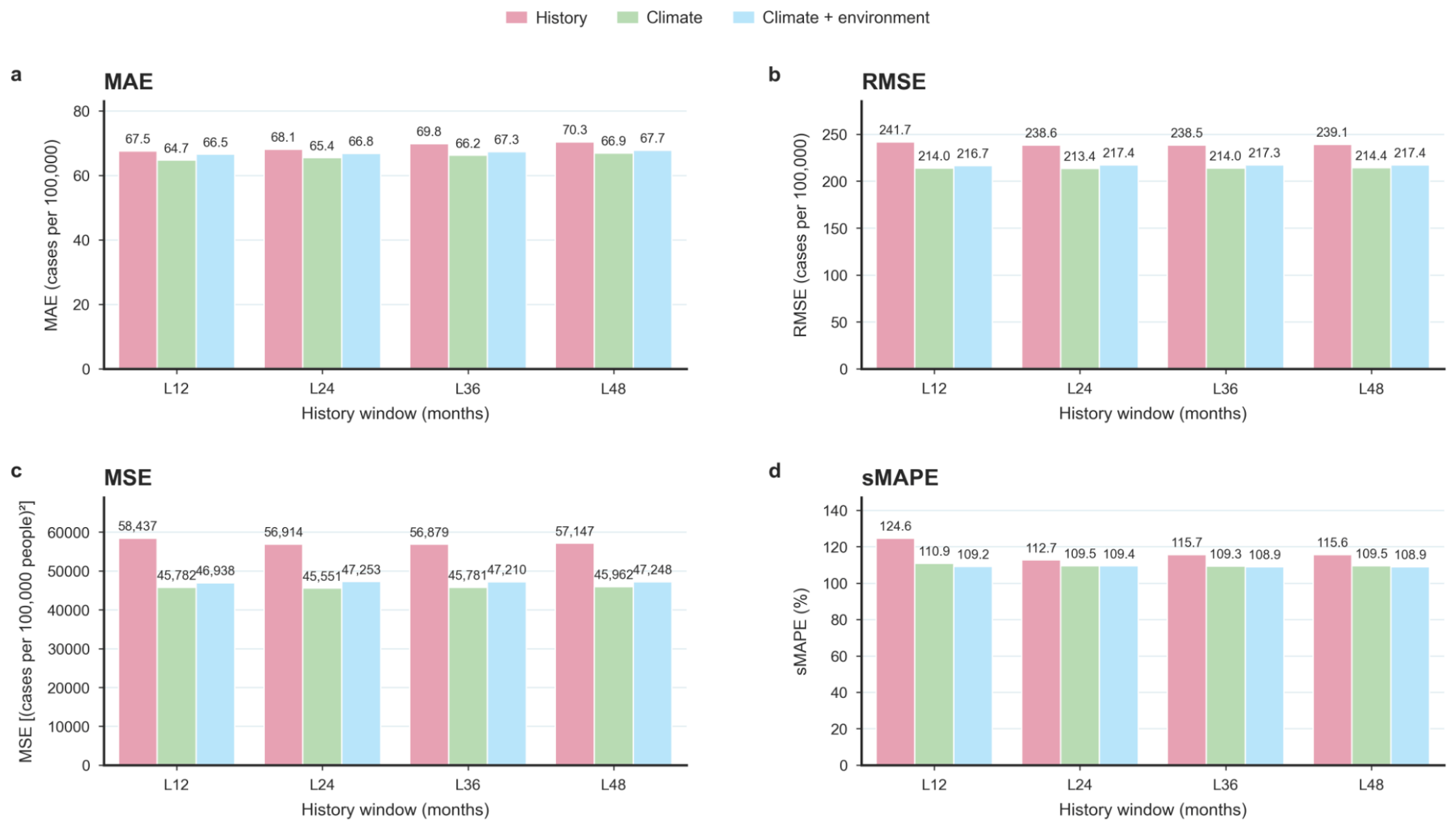
Figure 5.
The figure compares Stage 1 LightGBM environmental ablations with the validated climate inputs (Experiment 3B; per lookback). Lower values indicate better performance.
Figure 5.
The figure compares Stage 1 LightGBM environmental ablations with the validated climate inputs (Experiment 3B; per lookback). Lower values indicate better performance.
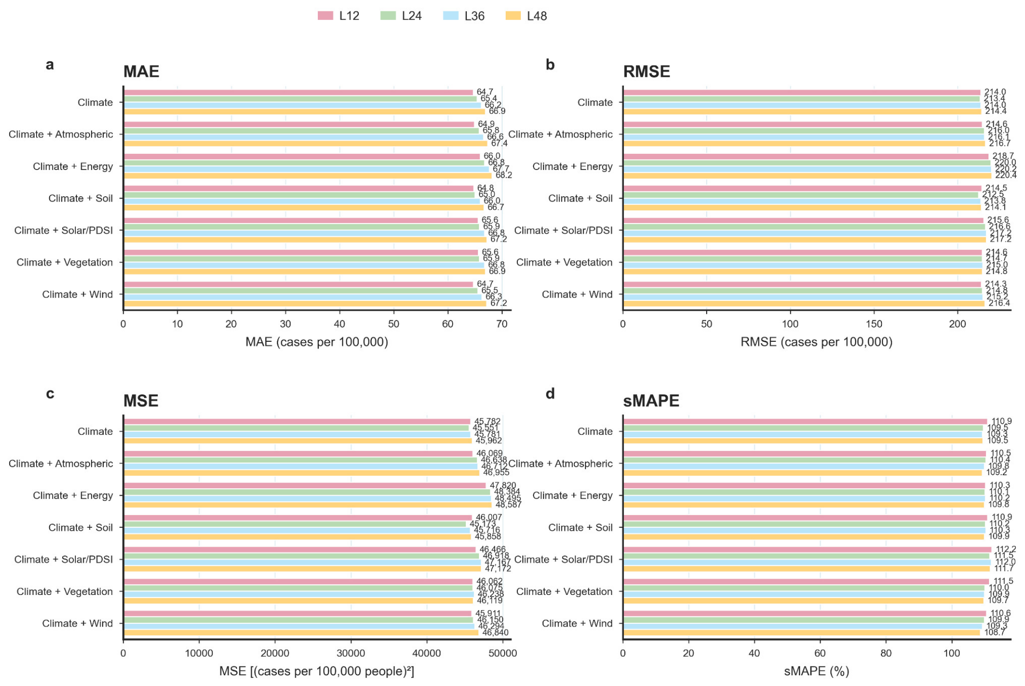
Figure 6.
The figure shows municipality-level G1 MAE improvement in corrected Experiment 4, averaged across two seeds. Positive values favor climate. The colors show the macroregions.
Figure 6.
The figure shows municipality-level G1 MAE improvement in corrected Experiment 4, averaged across two seeds. Positive values favor climate. The colors show the macroregions.
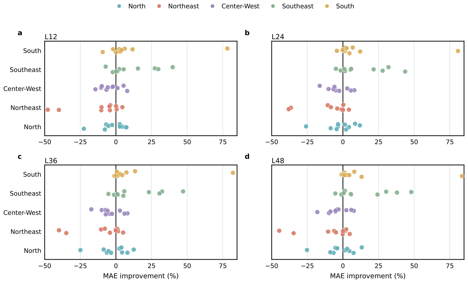
Figure 7.
The figure shows unweighted macroregion means of municipality-level G1 MAE improvement in corrected Experiment 4. Positive values favor climate. The averages are descriptive.
Figure 7.
The figure shows unweighted macroregion means of municipality-level G1 MAE improvement in corrected Experiment 4. Positive values favor climate. The averages are descriptive.
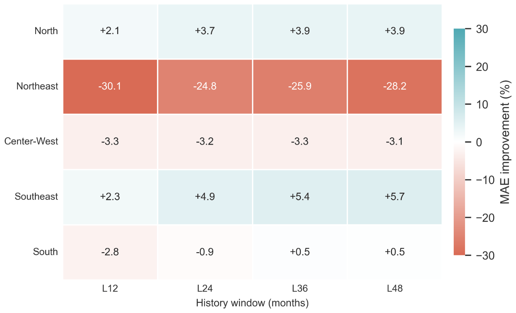
Figure 8.
The figure shows nationwide errors in retrospectively identified high-incidence months and pools three runs. The outcome-defined group is not a prospective outbreak class. Lower values indicate better performance. The TiDE-style results apply only to L12.
Figure 8.
The figure shows nationwide errors in retrospectively identified high-incidence months and pools three runs. The outcome-defined group is not a prospective outbreak class. Lower values indicate better performance. The TiDE-style results apply only to L12.
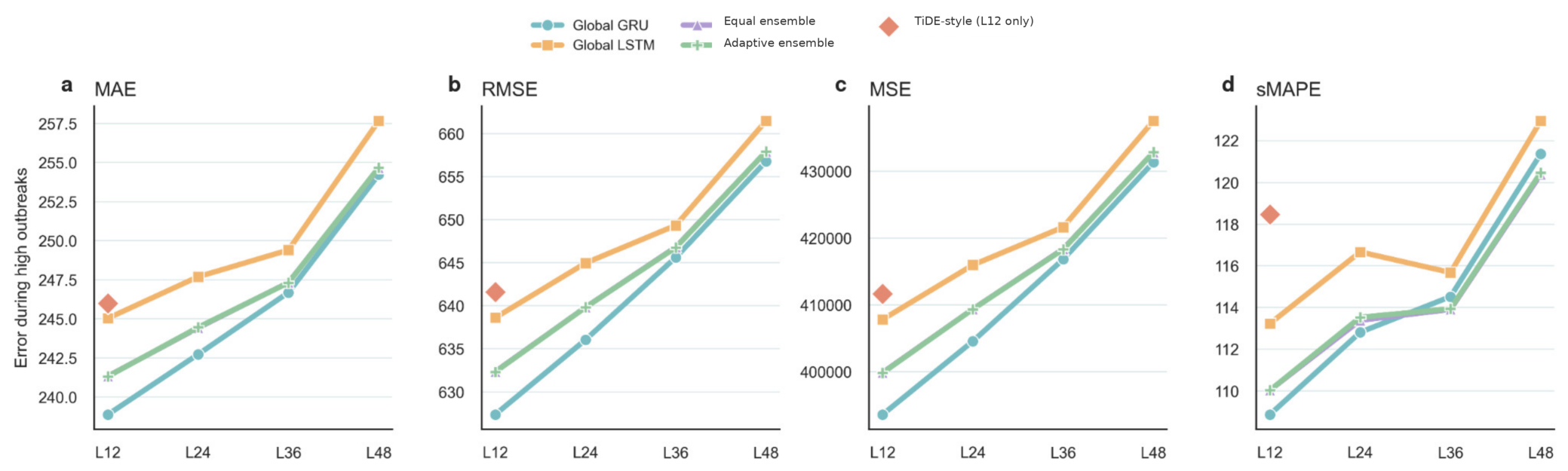
Figure 9.
The figure shows the nationwide L12 comparison. The bars average three run-specific pooled metrics ( each). We averaged MSE and RMSE separately. Lower values indicate better performance.
Figure 9.
The figure shows the nationwide L12 comparison. The bars average three run-specific pooled metrics ( each). We averaged MSE and RMSE separately. Lower values indicate better performance.
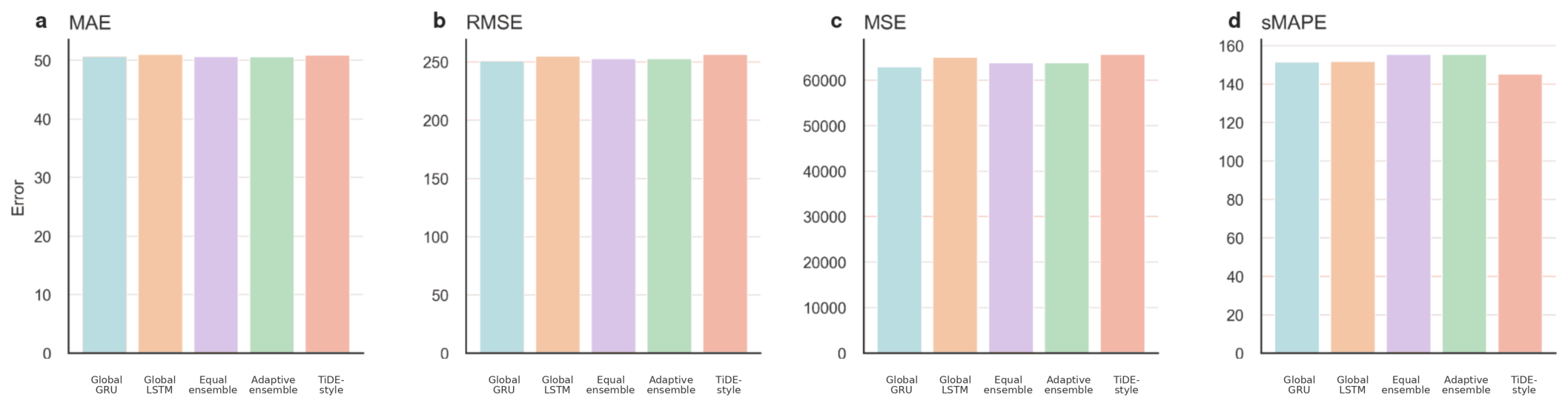
Table 2.
Experimental design and evidence map.
| Exp. | Question | Scope and protocol | Models and information | Evidence used in the manuscript |
|---|---|---|---|---|
| 1 | Does historical dengue incidence contain one-month-ahead predictive signal? | Stage 1; 50 municipalities; 60 rolling target months; –. | Seasonal Naive and Auto-SARIMA with fallback; historical incidence only. | Tests whether history alone provides a useful classical baseline. |
| 2 | Does shared cross-municipality learning outperform independent local training? | Stage 1; 50 municipalities; 60 rolling target months; –. | Local GRU versus Global GRU; history-only primary contrast. | Supports shared learning within Stage 1; it is not the nationwide validation. |
| 3A | Do climate or broader environmental covariates improve classical forecasting? | Stage 1; rolling one-month-ahead evaluation; comparisons use rows forecast successfully by both models. | History-only SARIMA, climate-SARIMAX, and climate-plus-environment SARIMAX with fixed orders. | Climate-SARIMAX gives mixed results. The unstable full-environment model shows a numerical failure but cannot be compared on performance. |
| 3B | Do climate and environmental covariates add value for nonlinear forecasting? | Stage 1; 50 municipalities; 60 rolling target months; –. | Local LightGBM: history only, history plus climate, and history plus climate plus environment; predefined ablations. | Climate improves the tested local LightGBM model; broader additions do not help consistently. |
| 4 | How do errors change after adding correctly aligned climate inputs to shared learning? | Stage 1; 50 municipalities; 60 rolling target months; –; two seeds. | G0 (history) and G1 (history plus 48 aligned climate features); matched targets and training but unequal parameter counts. | Climate changes errors differently by metric and municipality; it is not uniformly beneficial. |
| 5 | How do neural architectures compare under history-only inputs? | Stage 1; 50 municipalities; 60 rolling target months; –; three seeds. | G0 (Global GRU), L0 (Global LSTM), and T0 (Transformer); history-only conditions. | Architecture comparison. Climate-input variants are excluded because their alignment was not corrected. |
| 6 | Do retained history-only models scale nationwide? | Nationwide; 5,570 municipalities; 60 rolling target months; –; three base seeds. | G0, L0, equal ensemble, and adaptive ensemble. | Main nationwide internal validation; compares accuracy, high-incidence errors, coverage, and simplicity. |
| TiDE-style L12 | How does the implemented dense comparator behave nationwide at L12? | Nationwide; 5,570 municipalities; 60 rolling target months; only; three base seeds. | Archived TiDE-style history-only dense comparator. | Secondary sensitivity comparison. It lowers overall sMAPE and zero-target MAE/RMSE, but not overall MAE/RMSE or retrospective high-incidence error relative to G0. |
Notes: All experiments use one-month-ahead rolling origins and fitting-only preprocessing. Corrected Experiment 4 replaces the misaligned output. Later stages reuse 2019–2023 targets and therefore remain internal validation; climate/environment comparisons are descriptive, not causal.
Table 3A.
Historical predictability under rolling one-month-ahead evaluation (Experiment 1; Stage 1).
Table 3A.
Historical predictability under rolling one-month-ahead evaluation (Experiment 1; Stage 1).
| Lookback | Model | MAE | MSE | RMSE | sMAPE | n |
|---|---|---|---|---|---|---|
| 12 | Seasonal Naive | 84.665 | 95,766.9 | 309.462 | 84.045 | 3,000 |
| 12 | Auto-SARIMAa | 74.201 | 143,429.6 | 378.721 | 97.469 | 3,000 |
| 24 | Seasonal Naive | 84.665 | 95,766.9 | 309.462 | 84.045 | 3,000 |
| 24 | Auto-SARIMAa | 56.337 | 57,620.6 | 240.043 | 108.331 | 3,000 |
| 36 | Seasonal Naive | 84.665 | 95,766.9 | 309.462 | 84.045 | 3,000 |
| 36 | Auto-SARIMAa | 58.601 | 65,792.7 | 256.500 | 113.139 | 3,000 |
| 48 | Seasonal Naive | 84.665 | 95,766.9 | 309.462 | 84.045 | 3,000 |
| 48 | Auto-SARIMAa | 55.708 | 66,521.1 | 257.916 | 121.344 | 3,000 |
Each metric pools the paired municipality–target-month rows and gives every row equal weight. Lower values are better; n is the number of paired rows. RMSE is over those same rows.
Auto-SARIMA-with-fallback includes successful fits, deterministic all-zero and constant-window forecasts, and 97, 18, 3, and 1 Seasonal Naive fallback forecasts at L12–L48, respectively. No unresolved forecasts remained.
Table 3B.
Global versus local learning under rolling one-month-ahead evaluation (Experiment 2; Stage 1).
Table 3B.
Global versus local learning under rolling one-month-ahead evaluation (Experiment 2; Stage 1).
| Lookback | Model | MAE | MSE | RMSE | sMAPE | n |
|---|---|---|---|---|---|---|
| 12 | Local GRU | 75.034 | 55,976.0 | 236.592 | 160.675 | 3,000 |
| 12 | Global GRU | 57.416 | 38,346.8 | 195.823 | 154.890 | 3,000 |
| 24 | Local GRU | 75.180 | 56,697.5 | 238.112 | 160.551 | 3,000 |
| 24 | Global GRU | 56.787 | 37,444.9 | 193.507 | 154.796 | 3,000 |
| 36 | Local GRU | 74.596 | 54,564.7 | 233.590 | 161.035 | 3,000 |
| 36 | Global GRU | 57.455 | 38,390.1 | 195.934 | 155.265 | 3,000 |
| 48 | Local GRU | 75.042 | 56,126.5 | 236.910 | 160.911 | 3,000 |
| 48 | Global GRU | 57.152 | 38,592.9 | 196.450 | 154.879 | 3,000 |
Metrics pool 3,000 rows; lower is better and RMSE is . Global GRU lowers municipality-level MAE in 39/50, 39/50, 38/50, and 39/50 locations at L12–L48. This is a single recorded execution, so no inferential uncertainty is claimed.
Table 4.
Within-model changes after adding climate and broader environmental information in the fixed Stage 1 sample (incidence-rate units).
Table 4.
Within-model changes after adding climate and broader environmental information in the fixed Stage 1 sample (incidence-rate units).
| L12 | L24 | L36 | L48 | |||||
|---|---|---|---|---|---|---|---|---|
| Model and information set | MAE | RMSE | MAE | RMSE | MAE | RMSE | MAE | RMSE |
| Panel A: Local statistical models (Experiment 3A) | ||||||||
| M0: locked-order SARIMA–History | 76.619 | 384.932 | 57.943 | 243.477 | 60.901 | 261.593 | 56.803 | 260.569 |
| M1: locked-order SARIMAX–Climate | 94.420 | 550.829 | 57.360 | 238.000 | 57.805 | 249.282 | 51.918 | 239.291 |
| Panel B: Local nonlinear models (Experiment 3B; per lookback) | ||||||||
| LightGBM–History | 67.503 | 241.738 | 68.070 | 238.567 | 69.768 | 238.492 | 70.332 | 239.053 |
| LightGBM–Climate | 64.681 | 213.966 | 65.422 | 213.427 | 66.182 | 213.964 | 66.934 | 214.387 |
| LightGBM–Climate + environment | 66.514 | 216.651 | 66.805 | 217.378 | 67.281 | 217.278 | 67.726 | 217.365 |
Lower is better. Panel A uses common finite rows: , , , and at L12–L48. M2 is omitted because 3,674/12,000 forecasts were unusable and aggregate metrics were nonfinite.
Panel B has 3,000 rows per condition and lookback. Compare within panels only because model families and preprocessing differ. The Results section reports changes in sMAPE.
Table 5.
Corrected climate-input contrast after shared learning (Experiment 4; Stage 1).
| MAE | RMSE | sMAPE | MSE | Climate-input contrast | ||||||
|---|---|---|---|---|---|---|---|---|---|---|
| Lookback | G0 | G1 | G0 | G1 | G0 | G1 | G0 | G1 | MAEimprovement (%) | RMSEimprovement (%) |
| 12 | 57.145 | 59.595 | 196.835 | 197.135 | 148.430 | 120.288 | 38,748.6 | 38,862.8 | -4.30 | -0.16 |
| 24 | 58.003 | 59.426 | 197.748 | 197.394 | 148.297 | 119.680 | 39,107.8 | 38,964.9 | -2.45 | +0.17 |
| 36 | 58.390 | 59.640 | 198.134 | 197.673 | 148.361 | 119.914 | 39,259.2 | 39,075.1 | -2.14 | +0.23 |
| 48 | 58.256 | 59.592 | 197.953 | 197.631 | 148.168 | 119.782 | 39,188.1 | 39,058.4 | -2.29 | +0.15 |
Entries average two run-specific pooled metrics ( each). G1 adds 48 aligned climate features and has 3,233 versus G0’s 929 parameters. Lower is better.
Improvement is ; positive values favor G1. Mean MSE and mean RMSE are averaged separately. G1 wins municipality-level MAE in 27/50, 27/50, 28/50, and 29/50 locations. The two-seed comparison has no corresponding significance test.
Table 6A.
History-only fixed-configuration architecture comparison in Stage 1 (Experiment 5).
| Lookback | Model | MAE | RMSE | sMAPE | Parameters |
|---|---|---|---|---|---|
| 12 | Global GRU | 57.412 ± 0.698 | 196.812 ± 2.125 | 148.612 ± 0.565 | 929 |
| 12 | Global LSTM | 56.759 ± 0.996 | 198.431 ± 2.764 | 150.088 ± 0.640 | 1,233 |
| 12 | Transformer | 59.807 ± 4.162 | 209.354 ± 8.344 | 141.384 ± 2.709 | 18,241 |
| 24 | Global GRU | 58.155 ± 0.267 | 197.583 ± 1.809 | 148.669 ± 0.667 | 929 |
| 24 | Global LSTM | 58.069 ± 1.477 | 199.178 ± 3.417 | 150.847 ± 1.228 | 1,233 |
| 24 | Transformer | 61.759 ± 2.113 | 217.264 ± 5.142 | 139.571 ± 2.914 | 18,241 |
| 36 | Global GRU | 58.406 ± 0.422 | 197.876 ± 1.423 | 148.685 ± 0.612 | 929 |
| 36 | Global LSTM | 58.422 ± 1.767 | 199.986 ± 4.133 | 150.751 ± 1.188 | 1,233 |
| 36 | Transformer | 68.530 ± 9.175 | 227.030 ± 16.803 | 143.102 ± 7.620 | 18,241 |
| 48 | Global GRU | 58.314 ± 0.291 | 197.732 ± 1.596 | 148.536 ± 0.637 | 929 |
| 48 | Global LSTM | 57.908 ± 0.973 | 199.509 ± 3.510 | 150.701 ± 1.228 | 1,233 |
| 48 | Transformer | 73.544 ± 8.485 | 235.737 ± 20.746 | 144.632 ± 4.309 | 18,241 |
Means ± sample SD across three runs ( each). Parameter counts are unequal, so comparisons apply to the archived history-only configurations, not architecture alone.
Table 6B.
Nationwide internal validation of history-only shared models and simple combinations (Experiment 6).
Table 6B.
Nationwide internal validation of history-only shared models and simple combinations (Experiment 6).
| Lookback | Model | MAE | RMSE | sMAPE | n per seed |
|---|---|---|---|---|---|
| 12 | Global GRU | 334,200 | |||
| 12 | Global LSTM | 334,200 | |||
| 12 | Equal ensemble | 334,200 | |||
| 12 | Adaptive ensemble | 334,200 | |||
| 24 | Global GRU | 334,200 | |||
| 24 | Global LSTM | 334,200 | |||
| 24 | Equal ensemble | 334,200 | |||
| 24 | Adaptive ensemble | 334,200 | |||
| 36 | Global GRU | 334,200 | |||
| 36 | Global LSTM | 334,200 | |||
| 36 | Equal ensemble | 334,200 | |||
| 36 | Adaptive ensemble | 334,200 | |||
| 48 | Global GRU | 334,200 | |||
| 48 | Global LSTM | 334,200 | |||
| 48 | Equal ensemble | 334,200 | |||
| 48 | Adaptive ensemble | 334,200 |
Means ± sample SD across three runs; each run weights 334,200 rows equally. The adaptive ensemble uses earlier-target inverse-MAE weights and defaults to 0.5/0.5 weights when unavailable. MAE/RMSE use incidence per 100,000; sMAPE is percentage-scale.
Table 6C.
Nationwide L12 comparison of the archived TiDE-style dense comparator with the Global GRU.
Table 6C.
Nationwide L12 comparison of the archived TiDE-style dense comparator with the Global GRU.
| Condition | Model | MAE | RMSE | sMAPE |
|---|---|---|---|---|
| Overall, L12 | Global GRU | 50.709 ± 0.154 | 250.940 ± 0.446 | 151.543 ± 0.111 |
| Overall, L12 | TiDE-style dense | 50.935 ± 0.098 | 256.311 ± 0.465 | 145.215 ± 0.333 |
| High-incidence months | Global GRU | 238.877 | 627.363 | 108.870 |
| High-incidence months | TiDE-style dense | 245.988 | 641.597 | 118.463 |
| Positive, non-high | Global GRU | 31.506 | 68.015 | 90.320 |
| Positive, non-high | TiDE-style dense | 30.257 | 66.590 | 92.478 |
| Zero incidence | Global GRU | 10.232 | 28.217 | 184.561 |
| Zero incidence | TiDE-style dense | 9.258 | 26.675 | 171.133 |
The L12-only nationwide comparison covers three runs. Overall entries are means ± sample SD ( per run); strata pool runs across 52,168 high, 75,190 positive non-high, and 206,842 zero distinct targets.
Strata use observed outcomes and are retrospective. Zero-clipping affected 13.49% of dense and 6.32% of G0 forecasts. MAE/RMSE use incidence per 100,000; sMAPE is percentage-scale.
Disclaimer/Publisher’s Note: The statements, opinions and data contained in all publications are solely those of the individual author(s) and contributor(s) and not of MDPI and/or the editor(s). MDPI and/or the editor(s) disclaim responsibility for any injury to people or property resulting from any ideas, methods, instructions or products referred to in the content. |
© 2026 by the authors. Licensee MDPI, Basel, Switzerland. This article is an open access article distributed under the terms and conditions of the Creative Commons Attribution (CC BY) license (http://creativecommons.org/licenses/by/4.0/).
Copyright: This open access article is published under a Creative Commons CC BY 4.0 license, which permit the free download, distribution, and reuse, provided that the author and preprint are cited in any reuse.