

Submitted:
05 September 2026
Posted:
07 September 2026
You are already at the latest version
Abstract
Debt maturity composition is filed in every Italian balance sheet and rarely treated as an outcome. Using 73,662 firm-year observations on 11,265 unlisted firms over 2016–2024—innovative start-ups, innovative SMEs and ordinary SMEs drawn from one source on identical items—we estimate the effect of asset tangibility on the short-term share of debt. Maturity matching holds within firms and not only across them: the between coefficient is −0.380, the within coefficient −0.247, and instrumentation moves the estimate away from zero. Adjustment is incomplete, with persistence of 0.556 and a long-run response 1.8 times the static one. The relationship is steeply graded by regime, from −0.312 among ordinary SMEs to −0.120 among innovative start-ups. A taxonomy estimated without the regulatory register reproduces that gradient, indicating that certification selects balance sheets rather than shaping them. Flexible learners improve on the linear form by only 1.27 times.
Keywords:
debt maturity structure
; asset tangibility
; small and medium enterprises
; innovative start-ups
; panel data
1. Introduction
Research on small-firm debt has organised itself around two quantities. One is how much debt a firm carries, the other is what that debt costs. Both have been evaluated for Italian small firms with regression-discontinuity, survival and eligibility-threshold designs of a quality rarely achieved on administrative accounting data (Boschi, Girardi & Ventura, 2014; de Blasio et al., 2018; D’Ignazio & Menon, 2020; Lagazio, Persico & Querci, 2021). A third quantity sits in every filed balance sheet, is available for essentially every firm-year, and is almost never treated as an outcome: how the debt stock is distributed across maturities. It is orthogonal to the level by construction, since the same leverage is compatible with any mix of short and long claims, and orthogonal to the price by observation, since the same lender quotes different rates for the same borrower at different horizons.
This paper asks what determines that composition in a population of firms that cannot issue bonds, and takes as its focal regressor the variable the theory of maturity choice makes central: the share of the balance sheet held in fixed assets. The prediction is old and unambiguous: a firm finances long-lived assets with long-lived claims, either because refinancing a long asset at a date it does not choose is imprudent, or because fixed assets are what a bank will lend against for a decade. What is missing is not the theory but the evidence, and the gap has three components.
The first is population. Körner (2007), Cai, Fairchild and Guney (2008), Alcock, Finn and Tan (2012), Etudaiye-Muhtar, Ahmad and Matemilola (2017), Kalsie and Nagpal (2018), Vijayakumaran and Vijayakumaran (2019) and Phan (2020) span four continents and two decades, and are composed almost entirely of exchange-listed firms whose access to bond markets and rating agencies makes maturity a genuinely open choice. The refinements that followed—dispersion rather than average maturity, the profile rather than the level, the secular drift towards shorter debt (Gopalan, Song & Yerramilli, 2014; Choi, Hackbarth & Zechner, 2018; Byun, Lin & Wei, 2021; Clark & Park, 2023)—were made on the same population. The small-firm branch is thinner and reports the cross-sectional comparison as though it settled the within-firm one (Heyman, Deloof & Ooghe, 2008; Lopez-Gracia & Mestre-Barberá, 2015; Díaz-Díaz, García-Teruel & Martínez-Solano, 2016; D’Amato, 2020).
The second is the status of the regressor. Tangibility appears in the control vector of virtually every specification cited above, is consistently signed, and is virtually never the coefficient the paper is about. It is estimated hundreds of times without being interrogated once: rarely instrumented, rarely decomposed into its between and within parts, rarely tested for functional form, rarely measured twice.
The third is the outcome the collateral literature chooses. Work on pledgeability has moved quickly—enforcement costs and asset structure (Gopalan, Mukherjee & Singh, 2016), intangibles as collateral (Lim, Macias & Moeller, 2020), patent-pledging reforms (Dai et al., 2024; Chen et al., 2026; Wang, 2026)—but it asks whether a firm can borrow, how much and at what price. The horizon of the credit obtained is where the collateral mechanism should bite hardest, and it is left unexamined; Nakatani (2023) is among the few exceptions.
The setting allows a question that cannot be asked elsewhere. Innovative start-ups, innovative SMEs and ordinary SMEs are extracted from one source on identical items, so 73,662 firm-years on 11,265 firms over 2016–2024 can be compared across regimes without differential disclosure confounding the comparison. Three findings follow. Maturity matching is real inside firms and not only across them: the between coefficient is −0.380, the within coefficient −0.247. Adjustment is incomplete, with persistence bounded between 0.317 and 0.721 and a long-run response 1.8 times the static one. And the relationship is steeply graded by regime, from −0.312 among ordinary SMEs to −0.120 among innovative start-ups.
The design is what makes the third finding credible. A taxonomy estimated on nine accounting dimensions, with the regulatory register withheld entirely, reproduces the same gradient—evidence that certification selects balance sheets of a particular shape rather than creating it. Six flexible learners fitted to exactly the variation the fixed-effects estimator uses then improve on the linear form by a factor of 1.27, against the multiples of three to five such comparisons return on levels. The linear specification is shown adequate rather than assumed adequate—a claim panel papers ordinarily cannot make.
The article continues as follows. Section 2 reviews the literature on debt maturity, collateral and small-firm financing, and identifies the three gaps this study addresses. Section 3 describes the data and explains why three methods are used rather than one. Section 4 estimates the relationship across seven panel estimators and reports the dynamic and instrumented specifications. Section 5 partitions the same firms into a taxonomy of balance-sheet configurations and asks whether the coefficient of Section 4 describes one relationship or an average of several. Section 6 fits six flexible learners to the variation the fixed-effects estimator uses, to establish whether the linear form is adequate. Sections 7 to 10 discuss the results, draw the policy implications, state the limitations and conclude. Appendices A to C support the panel module, D to H the clustering exercise, and I to K the machine-learning validation.
2. Literature Review
What the maturity literature has established, and on whom. The modern treatment of debt maturity descends from two arguments made within a decade of each other. In the first, a firm that finances a long-lived asset with a short-lived claim exposes itself to refinancing at a date it does not choose, so the prudent policy is to match the maturity of liabilities to the maturity of assets. In the second, maturity is an instrument of governance: short debt disciplines managers by forcing them back to the credit market, and lenders shorten it precisely when they most doubt the borrower. Almost every empirical paper since has tested one of these two mechanisms, and the accumulated cross-sectional evidence is remarkably consistent in sign. Larger firms, more tangible firms and firms with better credit quality hold longer debt; growth options, information asymmetry and volatility shorten it. What the literature is far less consistent about is where that evidence comes from. Körner (2007) studies Czech firms, Cai, Fairchild and Guney (2008) Chinese ones, Alcock, Finn and Tan (2012) Australian ones, Etudaiye-Muhtar, Ahmad and Matemilola (2017) a panel of African countries, Kalsie and Nagpal (2018) NSE-listed Indian corporates, Vijayakumaran and Vijayakumaran (2019) Chinese listed companies, Phan (2020) listed Vietnamese enterprises, and Hussain, Shamsudin, Salehuddin and Jabarullah (2018) Malaysian shari’ah-compliant issuers. The list is long, geographically wide, and almost entirely composed of exchange-listed firms. Gopalan, Song and Yerramilli (2014), Choi, Hackbarth and Zechner (2018), Byun, Lin and Wei (2021) and Clark and Park (2023) refine the object of study—dispersion of maturities, the profile rather than the average, the secular drift towards shorter debt—but they refine it on the same population, whose access to bond markets, rating agencies and public equity makes the maturity decision a genuinely open choice. A second regularity concerns how tangibility enters. In this literature it is a control. It appears in the regressor vector of virtually every specification cited above, it is almost always signed negatively against the short-term share, and it is almost never the coefficient the paper is about. The consequence is that its magnitude is reported without being interrogated: rarely instrumented, rarely decomposed into its between and within components, rarely tested for functional form, and rarely measured in more than one way. A parameter that is estimated hundreds of times as a nuisance is not the same thing as a parameter that has been established.
Small firms, where the choice is narrower. The small-firm branch is more directly relevant and much thinner. Heyman, Deloof and Ooghe (2008) established for privately held Belgian firms that the determinants of financial structure differ from the listed benchmark; Lopez-Gracia and Mestre-Barberá (2015) show that agency conflicts operate on SME maturity through different channels than in large firms; Díaz-Díaz, García-Teruel and Martínez-Solano (2016) find that family control shifts maturity in Spanish private firms; Briozzo, Cardone-Riportella and García-Olalla (2019) and Dasilas (2024) trace governance attributes and credit ratings into the maturity and structure of non-listed SME debt. D’Amato (2020) is the closest antecedent to the present study, examining capital structure and debt maturity for SMEs across a financial crisis. More recently Gama and Vieira (2024) and Gama, Sol Murta and Vieira (2024) link conservative financing policies to societal trust and to the density of local bank branches, and Paeleman, Mataigne and Vanacker (2025) show that maturity structure, and not the debt level, predicts export withdrawal in international new ventures. Three limitations recur across this branch. Samples are small—typically a few thousand firm-years drawn from one country and a handful of years. Identification is cross-sectional or relies on short panels in which the within dimension is too thin to exploit, so the reported coefficient conflates the comparison between firms with the comparison of a firm against itself. And the dependent variable is usually a level of leverage with maturity treated as a secondary outcome, rather than the maturity composition treated as the object.
Collateral studied as access, not as horizon. The pledgeability literature has moved quickly and in a direction that makes the omission conspicuous. Gopalan, Mukherjee and Singh (2016) show that the cost of enforcing debt contracts shapes both financing and asset structure jointly. Lim, Macias and Moeller (2020) document that intangible assets support more debt than the collateral view predicts. Dai, Du, Gao, Gu and Wang (2024) and Wang (2026) exploit patent-pledging regimes in China to identify the effect of making a specific asset class collateralisable, and Chen, Pan, Qian, Wu and Xia (2026) push the same logic into innovation outcomes. Yang, Ma, Mi, Li and Chen (2026) go further still, treating collateral flexibility as an instrument for resolving maturity mismatch in supply-chain finance. The gap is precise. This literature asks whether a firm can borrow, how much, and at what price, and it establishes convincingly that pledgeable assets relax those margins. It rarely asks what happens to the horizon of the credit obtained. Yet the horizon is where the collateral mechanism should bite hardest: a bank will extend a five-year secured facility against a machine and a ninety-day revolving line against a receivable, so an asset-composition shock should show up in the maturity mix before it shows up in the leverage ratio. Nakatani (2023) is one of the few papers to connect the two explicitly, finding that debt maturity and productivity interact through the intangible share, and Deng and Liu (2024) and McGrattan (2020) supply the measurement apparatus for intangible capital that such work requires. Cortez (2025) surveys the emerging role of intangibles in capital-structure determination and reaches the same conclusion about what has not been done.
Maturity as regressor rather than outcome. A large body of work uses maturity as an explanatory variable. Dang (2011) and Kashefi Pour and Khansalar (2015) examine how leverage and maturity jointly govern investment and the underinvestment problem; Cutillas Gomariz and Sánchez Ballesta (2014) show that short maturity substitutes for reporting quality in disciplining investment; Khaw and Lee (2016), Wang, Wang and Xu (2022) and Nouman et al. (2023) trace maturity into investment efficiency and firm value under financial constraints; Petcharat and Mula (2026) and Li, Ye and Luo (2026) extend the design to ESG disclosure and earnings-forecast quality. On the risk side, Della Seta, Morellec and Zucchi (2020) model the risk-taking incentives created by short debt, Friewald, Nagler and Wagner (2022) price refinancing exposure in equity returns, He, Lütkebohmert and Xiao (2017) and Chaturvedi and Singh (2024) formalise rollover risk, and Huberman and Repullo (2025) return to the moral-hazard foundations. Wang, Chiu and King (2020), Chiu, King and Wang (2021) and Chu and Kjenstad (2023) establish that maturity and its dispersion are priced in loan spreads. Taken together this work makes the case that maturity composition matters for real and financial outcomes. It thereby raises, without answering, the question of what determines it in the population where the consequences are largest. It also proceeds almost universally from a static specification, imposing that maturity structure adjusts fully within the accounting year—an assumption that the persistence estimates reported in this paper reject.
Innovative firms and the Italian institutional setting. Two further literatures bear on the heterogeneity this study documents. The first concerns firms whose assets are largely uncollateralisable. Magri (2014) shows that equity issuance, not debt, supports R&D in unlisted Italian high-tech manufacturers; Hoffmann and Kleimeier (2021) price disclosure quality into innovative firms’ cost of debt; Castaldo, De Luca and Barile (2021) find that initial bank access predicts start-up default in Italy; Lee and Jung (2024), Liu and Chen (2023), Pisicoli, Marchionne and Beccari (2025) and Cattafi, Del Pozzo and Naciti (2025) examine the instruments—R&D human capital, banking deregulation, minibonds, green-innovation signalling—through which such firms obtain external finance. Haro-de-Rosario, Caba-Pérez and Cazorla-Papis (2016), Croce, Quas and Tenca (2025) and Runach, Garg and Narwal (2024) cover the venture-capital and bond alternatives. The second concerns the Italian bank–firm relationship and its public guarantee architecture, which has been evaluated with unusual rigour. Bartoli, Ferri, Murro and Rotondi (2013) and Gai, Ielasi and Rossolini (2016) study mutual guarantee institutions; Boschi, Girardi and Ventura (2014), de Blasio, De Mitri, D’Ignazio, Finaldi Russo and Stoppani (2018), D’Ignazio and Menon (2020), Caselli, Corbetta, Rossolini and Vecchi (2019), Caselli, Corbetta, Cucinelli and Rossolini (2021) and Lagazio, Persico and Querci (2021) evaluate the public schemes with regression-discontinuity, survival and eligibility-threshold designs; Corredera-Catalán, di Pietro and Trujillo-Ponce (2021) extend the comparison to Spain. Minetti, Murro, Rotondi and Zhu (2019), Fernández-Méndez and González (2019), Cerasi, Fedele and Miniaci (2017), Butzbach and Sarno (2019) and Falavigna, Ippoliti and Ramello (2026) document how local banking, ownership and judicial conditions shape credit terms.
These evaluations measure access, volume, cost and survival. None of them measures the horizon of the credit the guarantee delivers, which is the margin on which a scheme oriented towards short-term working-capital facilities would be expected to leave its clearest trace.
Method: taxonomies and validation. Finally, two methodological literatures are used rather than extended. João, Schaumburg, Lucas and Schwaab (2024) provide the reference treatment of nonparametric clustering on multivariate panel data; Gan and Valdez (2020) survey clustering in an actuarial-financial setting; Mikrou and Sapidis (2025) and Tran, Chang and Yu (2026) address the selection of algorithms and the role of validity indices; Viswanathan, Gopinathan and Rengasamy (2026) apply fuzzy clustering with membership diagnostics to bank ratings; Pongvijan and Trakunphutthirak (2026) argue for multi-metric rather than single-index evaluation; Xiang (2025) illustrates the single-algorithm, single-index practice that remains common in applied finance. On the regression side, Sinha and Vodwal (2023), Neves, Serrasqueiro, Dias and Hermano (2020), Haron et al. (2021), Canofari, Cucculelli, Piergallini and Renghini (2025), Iwaki (2019), Yuan (2026) and Paseda, Ashade, Manasseh and Olurin (2026) supply the panel and system-GMM practice this study follows. The common weakness is that flexible learners enter applied finance almost exclusively as predictors. They are rarely turned back on the econometric model to ask whether its functional form is adequate—which is the use made of them here.
The gap this study occupies. Placing the six strands side by side identifies a specific vacancy rather than a general one. The maturity literature has a well-developed theory, a stable set of cross-sectional findings and almost no evidence from firms that cannot issue bonds. The small-firm literature has the right population but reports the between comparison as though it were the within one. The collateral literature has the right regressor and the wrong outcome, having established what pledgeable assets do to the availability and price of credit while leaving its horizon unexamined. The investment literature treats maturity as given. The innovation-finance and guarantee literatures describe exactly the institutional environment in which the certified Italian populations operate, and measure every margin of credit except its term. And the methodological literatures supply tools—panel taxonomies, validity-index ensembles, flexible learners—that applied finance uses for description and prediction rather than for testing the specification it has already estimated. What follows occupies that vacancy on four fronts. It makes debt-maturity composition the dependent variable in a population of 11,265 unlisted Italian firms observed for up to nine years, of which two-fifths are certified innovative start-ups or innovative SMEs and the remainder ordinary SMEs extracted from the same source on identical items. It makes asset tangibility the focal regressor rather than a control, and measures both focal variables twice by independent routes through the balance sheet before estimating anything. It separates the between from the within comparison and reports both, then bounds the speed of adjustment that the static specification suppresses. And it subjects the resulting linear equation to two disciplines it did not choose: a taxonomy of balance-sheet configurations estimated without reference to the equation or to the regulatory register, and a battery of flexible learners fitted to exactly the variation the fixed-effects estimator uses. Neither discipline is decorative. The first shows that the regime heterogeneity is recoverable from accounts alone, which weakens the reading that certification itself produces it. The second shows that the flexible learners improve on the linear fit by a factor of 1.27 rather than the multiples of three to five that the same procedures return on levels—evidence that the functional form imposed in the panel module is adequate rather than convenient. See Table 1.
3. Data and Methodology
The data come from three extractions of AIDA (Bureau van Dijk), which harmonises the filed accounts of Italian limited companies. Innovative start-ups and innovative SMEs are drawn from the two special sections of the Business Register; ordinary SMEs from a comparison extraction of non-certified firms. All three share an identical variable structure, so every item is available for every group—the condition that makes a three-regime comparison meaningful rather than an artefact of differing disclosure. The estimation sample is 73,662 firm-year observations on 11,265 firms over 2016–2024: 2,213 innovative start-ups, 2,763 innovative SMEs and 6,289 ordinary SMEs. Continuous variables are winsorised at the first and ninety-ninth percentiles within year, and standard errors are clustered at firm level throughout.
The dependent variable is the short-term share of total debt, filed for 99.3 per cent of accounts. Tangibility is fixed assets over total assets, recovered exactly from the structural margin. Both are constructed twice by independent balance-sheet routes and the versions correlate at 0.984 and 0.666—a check the maturity literature does not ordinarily perform, and one that matters here because the sign instability reported across studies of private firms (Heyman, Deloof & Ooghe, 2008; D’Amato, 2020) is plausibly a measurement problem as much as an economic one.
Each module answers a question the others cannot, and the design is sequential rather than parallel.
The panel module estimates the coefficient. Pooled OLS, between, random effects, fixed effects, two-way fixed effects and two weighted variants are reported side by side because the between–within comparison is the diagnostic the SME literature omits: cross-sectional studies of private firms (Díaz-Díaz, García-Teruel & Martínez-Solano, 2016; Briozzo, Cardone-Riportella & García-Olalla, 2019) report the first and imply the second. A dynamic specification follows the bounding logic standard in this literature (Sinha & Vodwal, 2023; Neves, Serrasqueiro, Dias & Hermano, 2020), because the static form imposes full within-year adjustment. Instrumental variables address the simultaneity that the pledgeability literature identifies through policy shocks (Dai, Du, Gao, Gu & Wang, 2024; Wang, 2026) and which is unavailable here.
The clustering module asks whether one coefficient describes one relationship. A sample split chosen by the researcher inherits the hypothesis it tests; a taxonomy estimated on nine balance-sheet dimensions with the regulatory register withheld does not. Six algorithm families are compared on eleven validity indices with rank aggregation, following the multi-metric argument of Pongvijan and Trakunphutthirak (2026) and Mikrou and Sapidis (2025) against the single-index practice still common in applied finance, and drawing on panel-clustering (João, Schaumburg, Lucas & Schwaab, 2024) and financial-clustering (Gan & Valdez, 2020; Viswanathan, Gopinathan & Rengasamy, 2026) precedents.
The machine-learning module asks whether the functional form holds. Six learners are fitted to the same equation under three transformations—levels, Mundlak and firm- and year-demeaned—so that the comparison is against the variation the fixed-effects estimator actually uses. Cross-validation is grouped by firm. The purpose is validation, not prediction.
The structure is therefore cumulative: the first module produces a number, the second tests whether it is an average of heterogeneous relationships, the third tests whether the form that produced it is adequate. See Figure 1.
4. Debt Maturity and Asset Tangibility
Almost everything written about small-firm debt concerns two quantities: how much of it there is, and what it costs. A third quantity is measured in every filed account and is almost never used as an outcome—the composition of the debt stock across maturities. It is orthogonal to the level by construction, since a firm can hold the same leverage with any mix of short and long claims, and orthogonal to the price, since the same lender charges different rates for the same borrower at different horizons. This section asks what determines that composition, and takes as the focal regressor the variable the theory of maturity choice makes central and the empirical literature on Italian small firms has left almost untouched: the share of the balance sheet held in fixed assets.
The prediction is old and unambiguous. Under the matching principle of Myers (1977) and Hart and Moore (1994), a firm finances long-lived assets with long-lived claims, because a short claim against a long asset forces refinancing at a moment the borrower does not choose. Under the collateral reading of Barclay and Smith (1995), the same correlation arises for a different reason: fixed assets are what a bank will lend against for ten years, and a firm without them cannot obtain a ten-year loan whether or not it wants one. The two mechanisms are observationally close and this design does not separate them; what it does establish is whether the association survives the removal of firm heterogeneity, which is where most of the cross-sectional evidence has never been taken. See Table 2.
Neither variable required reconstruction and neither is shared with any dependent variable used elsewhere in this project. The maturity index is filed for 99.3 per cent of accounts, and fixed assets follow exactly from the structural margin, which is net worth minus fixed assets by definition. Both constructions were checked against an independent second route through the financial coverage ratio and the amortisation mix; the two versions of the dependent variable correlate at 0.984, and Appendix A reports the comparison. The distributions are described in Appendix A as well, and one feature of them matters for reading what follows: 31.3 per cent of firm-years hold no long-term debt at all, so the dependent variable piles up at its upper bound.
The first question is which estimator the data impose, and the answer is unambiguous in all three directions. The F test on joint significance of the individual effects is 9.31 and rejects; the Breusch–Pagan multiplier is 65,218.6; the Hausman statistic on four degrees of freedom is 313.96. Pooled OLS and random effects are both rejected, and two-way fixed effects is the reference specification. See Table 3.
The table reports one column per estimator; the figure places all seven on a common axis, so the distance between the cross-sectional and the within-firm readings of the same coefficient becomes visible. See Figure 2.
The coefficient is negative under every estimator and never comes close to zero. What Figure 1 makes visible is the size of the gap between the two extremes of the variance decomposition. Across firms the slope is −0.380: a firm holding ten percentage points more of its assets in fixed form finances 3.8 percentage points less of its debt at short maturity. Within firms it is −0.247. Roughly two-thirds of the cross-sectional gradient is reproduced when the firm is compared only with itself, which is a strong result by the standards of a literature that has almost always reported the first number and left the second unexamined. The remaining third is composition: firms that are permanently asset-heavy differ from firms that are permanently asset-light in ways the equation does not contain, and part of the raw correlation belongs to those differences rather than to the balance-sheet mechanism.
Scaled to the variation the fixed-effects estimator actually uses, the within coefficient implies that a one-standard-deviation increase in tangibility inside a firm—9.6 percentage points—shifts 2.3 percentage points of the debt stock out of short maturity, which is 18.9 per cent of a within-firm standard deviation of the dependent variable. That is a moderate effect, not a dominant one, and the honest statement is that asset composition moves maturity composition materially without determining it.
One objection to everything above is that the dependent variable is a proportion. It is bounded at zero and one, 31.3 per cent of firm-years sit exactly at the upper bound, and a linear model fitted to such a variable can in principle predict outside the admissible range and can misstate marginal effects near the boundary. The specification is therefore re-estimated as a fractional response model in the manner of Papke and Wooldridge, with a probit link, quasi-maximum likelihood, and a Mundlak correction that adds the firm mean of every time-varying regressor so that the estimator remains consistent under correlation between the effects and the covariates. Year effects and firm-clustered standard errors are retained. The joint test on the four firm means is decisive, χ²(4) = 609.2, which confirms that the correlated random-effects specification is required rather than optional and reproduces the ssmessage of the Hausman test in the linear setting.

Table 4.
Fractional response estimates with Mundlak correction.
| Index coefficient | Average partial effect | z | Linear benchmark | |
|---|---|---|---|---|
| TANG | −0.8425*** (0.0332) | −0.2144*** (0.0084) | −25.39 | −0.2410*** (0.0102) |
| SIZE | −0.1683*** (0.0095) | −0.0428*** (0.0024) | −17.71 | −0.0437*** (0.0025) |
| COVER | 0.0255*** (0.0015) | 0.0065*** (0.0004) | 16.69 | 0.0069*** (0.0004) |
| GROWTH | 0.0406*** (0.0052) | 0.0103*** (0.0013) | 7.78 | 0.0103*** (0.0015) |
| Mundlak test, χ²(4) | 609.2*** | |||
| Observations | 73,662 | |||
| Firms | 11,265 |
Note. Dependent variable: short-term debt over total debt. Fractional probit estimated by quasi-maximum likelihood with the firm mean of each time-varying regressor added as a Mundlak correction, year effects, and standard errors clustered at firm level, reported in parentheses. *** p < 0.01, ** p < 0.05, * p < 0.10. Average partial effects are computed over the estimation sample with standard errors obtained by the delta method. The linear benchmark is the two-way fixed-effects specification of Table 3. The Mundlak test is the joint hypothesis that the four firm means are zero.
The two columns agree. The average partial effect of tangibility is −0.214 against a linear estimate of −0.241: the same sign, the same order of magnitude, and a difference of 0.027 that is about two and a half standard errors of the fractional estimate. The three controls are indistinguishable across the two specifications to the third decimal. The reason the linear model performs this well despite the mass point is visible in the fitted values: only 0.72 per cent of them fall outside the unit interval, because the conditional mean over most of the covariate space is far from either boundary and the pile-up at unity reflects firms that hold no long-term debt rather than a censoring of an underlying latent variable. The regime gradient also survives the change of functional form, with average partial effects of −0.269 for ordinary SMEs, −0.171 for innovative SMEs and −0.110 for innovative start-ups, against −0.312, −0.177 and −0.120 in the linear specifications of Appendix B.
Two implications follow. First, the reported coefficient is not an artefact of imposing linearity on a bounded outcome, which is the concern the boundedness raises. Second, the linear estimate is if anything the more conservative of the two in the direction that matters for the regime comparison, since the fractional model compresses the ordinary-SME slope more than the certified ones and therefore narrows the gap the article emphasises. The linear specification is retained as the baseline because it is directly comparable with the between, dynamic and instrumented estimates that follow, none of which has a standard fractional counterpart.
The controls behave as the same theory requires. Larger firms hold less short-term debt, and the size coefficient is six times larger within firms than across them (−0.0437 against −0.0091), meaning that growth in a firm’s own asset base opens access to long maturities in a way that being structurally large does not capture. Better interest coverage is associated with more short-term debt, not less, which is the sign the refinancing-risk argument predicts: a firm that comfortably services its charges can bear the rollover exposure that a fragile one cannot. Revenue growth pushes weakly in the same direction.
One asymmetry inside the sample deserves recording here rather than only in the appendix, because it is the finding most specific to these populations. Estimating the same within-firm equation separately on the three regulatory groups gives −0.312 for ordinary SMEs, −0.177 for innovative SMEs and −0.120 for innovative start-ups, and a single pooled equation with regime interactions rejects equality of all three slopes at one per cent. The ordering is not a size effect in disguise: the split by size in Appendix B moves the coefficient far less than the split by regime, and the certified firms are on average younger and smaller but also more liquid and less levered. What the gradient says is that maturity matching is a choice, and choosing requires a long-maturity market to be open. A firm whose balance sheet is thin in collateralisable assets, and whose bank credit arrives largely through short-horizon lines carrying a public guarantee, faces a narrower menu, and its maturity structure responds correspondingly less to what it happens to hold in fixed form. Read across the decade the same logic appears in the time dimension, where the cross-sectional slope weakens monotonically from −0.400 in 2016 to −0.348 in 2024.
Two things the static equation cannot do are done in the appendix. It imposes that maturity structure adjusts fully within the year, and it does not. Bounding the coefficient on the lagged dependent variable between the two estimators whose bias is signed places persistence between 0.317 and 0.721; the Anderson–Hsiao estimate of 0.556 lies inside that interval, and the accumulated response to tangibility is −0.437, roughly 1.8 times the static one. And the static equation is associational. Instrumenting the second and third lags of tangibility in first differences returns −0.332 and −0.398 against a first-differenced least-squares benchmark of −0.211, with first-stage F statistics above 979 and a Hansen J of 1.25 at p = 0.263; adding the accumulated depreciation ratio as a third instrument leaves the overidentification test at p = 0.827. Instrumentation therefore moves the estimate away from zero rather than towards it, which is what classical measurement error in a differenced regressor implies, and corroborates the sign without identifying it—the supply-side peer instruments that would have identified it are too weakly correlated with the regressor to be informative, and Appendix C reports them as failures rather than suppressing them.
5. A Taxonomy of Balance-Sheet Configurations
The panel section returned one number for the association between asset composition and debt maturity, and the number is an average. Whether it is the average of one relationship or of several is not something the equation can answer, because the split that would settle it would have to be chosen by the person estimating the equation, and any split chosen that way inherits the hypothesis it is meant to test. This section takes the alternative route. It partitions the same firms on their balance-sheet configuration alone, with the outcome variable of interest treated as one dimension among nine and with the regulatory label withheld entirely, and only afterwards asks whether the groups the data produce differ in the relationship the previous section estimated.
The unit of clustering is the firm rather than the firm-year, because a taxonomy whose members change every year is not a taxonomy; each firm enters as the mean of its own observations over the nine years, and the sample is exactly the 11,265 firms of the panel. The nine dimensions are the nine analysis variables, standardised to zero mean and unit variance so that no dimension dominates by its scale. Six families of algorithms were fitted at five clusters: centroid partitioning, model-based mixture, fuzzy partitioning, agglomerative hierarchy, density-based clustering and an unsupervised random forest. The number five is defended in Appendix D; the short version is that variance explained rises smoothly with no elbow, the information criteria fall monotonically, and the entropy of cluster sizes peaks in the range six to seven, so the choice is a judgement about interpretability rather than a discovery, and it is held fixed across all six algorithms so that the comparison is between algorithms and not between granularities. See Table 5.
Eleven validity indices were computed on every solution, in the same nine-dimensional space and on a common five-thousand-firm subsample wherever a full distance matrix would have been required. They fall into four groups that do not measure the same thing, which is the reason for using all of them: variance criteria (R², Calinski–Harabasz), likelihood criteria (AIC, BIC), geometric criteria (silhouette, maximum diameter, minimum separation, Dunn, Pearson gamma) and balance criteria (the entropy of the size distribution and its Herfindahl–Hirschman concentration). See Table 6.
Reading eleven indices down a column is laborious. The figure recodes each cell by its rank, so the pattern that produces the aggregate ordering becomes visible at a glance. See Figure 3.
The last row of Table 5 is the reason the exercise uses eleven indices rather than one. The density-based solution wins the silhouette outright at 0.250, wins the Dunn index by a factor of four, wins the minimum separation by a factor of nearly three, has the smallest maximum diameter and the lowest information criteria in the table—and it achieves all of this by refusing to classify 35.8 per cent of the firms and by dividing the remainder into two groups that explain 0.4 per cent of the variance. Every geometric index rewards it precisely because discarding the firms that sit between groups is what makes the surviving groups compact and separated. The variance and balance criteria expose it: R² of 0.004, Calinski–Harabasz of 14 against 905 for K-means, a Herfindahl of 0.539. A selection rule built on any single geometric index would have chosen the least informative partition in the set.
Aggregating ranks across all eleven indices puts fuzzy C-means first at a mean rank of 2.62, K-means second at 2.88 and Ward third at 3.17, with the density-based solution fourth precisely because its geometric victories are offset by its balance and variance failures. The gap between the top three is small and none of the substantive results below changes if K-means is substituted; fuzzy C-means is selected because it is first on the aggregate, because it dominates K-means on minimum separation, Dunn, entropy and concentration while conceding only R² and silhouette by two thousandths, and because the membership degrees it produces make the fuzziness of the partition observable rather than hidden. See Figure 4.
The two components account for 47.2 per cent of total variance and identify what the taxonomy is organised around. The first contrasts interest coverage, profitability, capital turnover and short-term debt against tangibility—an operating-intensity axis, running from asset-heavy and slow to asset-light and fast. The second contrasts liquidity against leverage, with size loading negatively on both—a financial-structure axis. Neither is a size axis, which matters: the groups are not a disguised sorting by scale. See Table 7.
Table 7.
Cluster profiles.
| C0 Loss-making asset builders | C1 Young and asset-light | C2 Levered traders | C3 Capitalised performers | C4 Capital-intensive | |
|---|---|---|---|---|---|
| Firms | 1,293 | 2,019 | 2,942 | 2,150 | 2,861 |
| Share of sample | 11.5% | 17.9% | 26.1% | 19.1% | 25.4% |
| Short-term share | 0.724 | 0.881 | 0.890 | 0.890 | 0.653 |
| Tangibility | 0.461 | 0.217 | 0.157 | 0.231 | 0.475 |
| ln total assets | 6.58 | 5.29 | 8.42 | 8.97 | 8.91 |
| Interest coverage | −1.89 | 3.09 | 3.22 | 5.38 | 2.64 |
| Revenue growth | 0.612 | 0.643 | 0.178 | 0.103 | 0.129 |
| Leverage | 0.533 | 0.615 | 0.818 | 0.434 | 0.710 |
| Liquidity | 2.33 | 2.01 | 1.26 | 2.81 | 1.20 |
| Capital turnover | 0.45 | 1.15 | 1.76 | 1.03 | 0.82 |
| Return on assets | −19.03 | 11.92 | 5.59 | 12.37 | 3.22 |
| Certified share | 91.9% | 92.6% | 14.1% | 26.7% | 32.5% |
Note. Means of firm averages on the raw scale. “Certified share” is the proportion of innovative start-ups and innovative SMEs; the regulatory label took no part in the clustering.
Table 8.
The panel equation estimated inside each cluster.
| Cluster | β (TANG) | SE | Obs. | Firms | R² within |
|---|---|---|---|---|---|
| C0 Loss-making asset builders | −0.0890*** | (0.0308) | 5,566 | 1,293 | 0.033 |
| C1 Young and asset-light | −0.1728*** | (0.0237) | 8,602 | 2,019 | 0.069 |
| C2 Levered traders | −0.2574*** | (0.0189) | 21,303 | 2,942 | 0.097 |
| C3 Capitalised performers | −0.2373*** | (0.0219) | 16,746 | 2,150 | 0.124 |
| C4 Capital-intensive | −0.2902*** | (0.0193) | 21,445 | 2,861 | 0.130 |
| All firms | −0.2410*** | (0.0102) | 73,662 | 11,265 | 0.092 |
Note. Dependent variable: short-term debt over total debt. Each row is a separate two-way fixed-effects regression estimated on the firms assigned to that cluster, with the controls of Table 3 (SIZE, COVER, GROWTH) and standard errors clustered at firm level, reported in parentheses. *** p < 0.01, ** p < 0.05, * p < 0.10. Clusters are the fuzzy C-means solution of Table 6, estimated on nine standardised balance-sheet dimensions with the regulatory register withheld. The five cluster slopes are not equal: a pooled equation with cluster interactions rejects equality with a Wald statistic of 56.36 on four degrees of freedom (p < 0.001). Because the clusters were formed on dimensions that include both variables entering the equation, the slope differences are descriptive rather than an out-of-sample test.
This is the result the section exists to deliver. A taxonomy estimated with no knowledge of the regulatory status of any firm, and with the dependent variable entering as one of nine equally weighted dimensions, reproduces the ordering that the regime split of the panel section produced. The two clusters that are more than nine-tenths certified, C0 and C1, carry the flattest maturity-matching slopes at −0.089 and −0.173; the three clusters dominated by ordinary SMEs carry slopes between −0.237 and −0.290. The steepest is C4, where tangibility averages 0.475 and only 65 per cent of debt is short-term—firms that hold long assets and have arranged long liabilities against them. The flattest is C0, where tangibility is almost as high, at 0.461, but interest coverage is negative and return on assets is −19 per cent: firms that own the collateral and cannot use it, because a lender does not extend a ten-year claim against a borrower who is not covering this year’s charges. Maturity matching, on this evidence, is not a mechanical property of the asset side. It requires both the assets and the standing to borrow against them, and the taxonomy separates the firms that have both from the firms that have only the first.
It is worth being precise about what this does and does not establish. The clusters were built on nine dimensions that include both variables entering the equation, so the slope differences in Table 4 are not an out-of-sample validation and no causal weight attaches to them. What they do rule out is a specific alternative account of the panel result. If the flatter slope among certified firms were produced by the certification process itself—by selection into the register, by the reporting incentives it creates, or by the guarantee schemes attached to it—then a partition built from accounting data alone, blind to the register, would have no reason to reproduce it. It reproduces it exactly: the correlation between a cluster’s certified share and its maturity-matching slope is monotone across all five groups. The more economical explanation is that certification selects firms whose balance sheets already have this shape, and that the shape, not the certificate, is what flattens the slope.
One qualification belongs here rather than in the appendix. The partition is genuinely fuzzy: the mean maximum membership degree is 0.603 and 52.1 per cent of firms have a leading membership below 0.6, so the majority of firms sit somewhere between two configurations rather than inside one. The boundaries are soft, the centres are not, and Appendix G shows that the five centres are stable across bootstrap replication with cluster-wise Jaccard between 0.88 and 0.95.
6. Machine-Learning Regression as a Validation of the Panel Model
The panel estimates rest on an assumption that the estimates themselves cannot test: that every regressor enters linearly and that their effects add. If the true surface curves, or if tangibility matters more when coverage is weak, the fixed-effects coefficient is an average over a structure it does not describe, and nothing in a t statistic would reveal it. This section tests the assumption on the same equation, the same four regressors and the same 73,662 observations, using flexible learners whose accuracy is measured out of sample. The purpose is neither prediction nor identification. It is to establish how much systematic variation the linear form fails to capture, which variables carry it, and whether the omission can be repaired inside a parametric model. Cross-validation is five-fold and grouped by firm, so no firm contributes to both training and testing and the reported accuracy is not inflated by the panel structure.
One comparison made routinely in applied work is invalid, and correcting it changes the size of the result by more than the choice of learner does. The fixed-effects estimator explains variation within firms, after firm and year means have been removed; a learner fitted to raw levels also has the between-firm variation available, which in these data is the larger part. Setting a within R² of 0.075 against a levels R² of 0.290 attributes to functional form what is mostly a different variance decomposition. The two must be placed on the same footing, so every learner is fitted three times: on levels, on levels augmented with firm means in the manner of Mundlak, and on firm- and year-demeaned data, which is exactly what the two-way fixed-effects estimator uses. See Table 9.
Figure 5.
Out-of-sample accuracy of six learners under three variance decompositions. Note. Five-fold cross-validation grouped by firm; bars are means across folds and whiskers are one standard deviation. Right: the linear model against the best learner on each footing, with the ratio above each pair.
Figure 5.
Out-of-sample accuracy of six learners under three variance decompositions. Note. Five-fold cross-validation grouped by firm; bars are means across folds and whiskers are one standard deviation. Right: the linear model against the best learner on each footing, with the ratio above each pair.
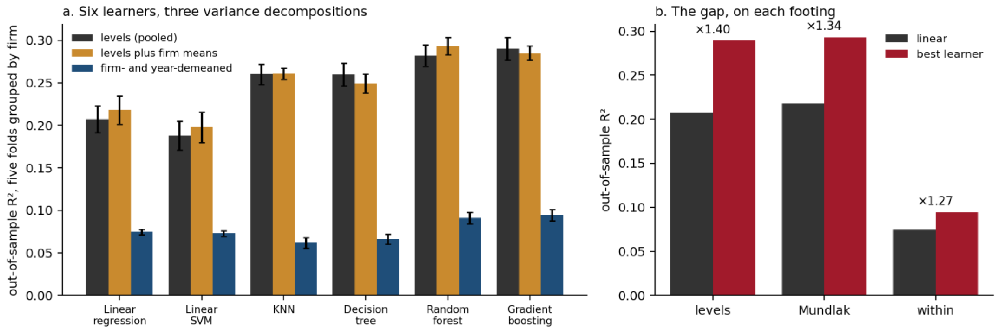
On raw levels the non-linear model is 1.40 times more accurate; on the data the fixed-effects estimator actually uses, the ratio falls to 1.27 and the absolute gap falls from 0.083 to 0.020. The honest statement is that the linear specification recovers 0.075 of within-firm variance against 0.095 attainable, not 0.207 against 0.290. Supplying the linear model with firm means as additional regressors raises it only from 0.207 to 0.218, so the between-firm information the learners exploit is itself non-linear in those means—which is a statement about cross-sectional heterogeneity, not about the within-firm relationship this study estimates. See Table 10.
Two features of this table matter more than the ranking. The first is that two of the four flexible learners are worse than the linear model: a single decision tree recovers 0.066 and nearest neighbours 0.062, against 0.075 for least squares. A learner that can represent any function and still loses to a plane is telling us there is little curvature to find and a great deal of noise to overfit—the nearest-neighbour in-sample R² of 1.000 against 0.062 out of sample is that diagnosis in its purest form. The second is that the linear model and the linear support-vector machine, which differ only in loss function, agree to within 0.002, so nothing in the result depends on squared-error loss or on the influence of outlying observations. Gradient boosting is selected as the reference non-linear model: it is the most accurate, it has the smallest overfitting gap of the four flexible learners, and it is roughly forty times faster to fit than the random forest that comes second. See Figure 6.
The validation proper is in the right panel. If the linear form were hiding a threshold, a saturation or a reversal in the focal relationship, the boosting curve would depart from the dashed line, and it does not: the two are almost indistinguishable over the central four-fifths of the distribution, with mild flattening only in the extreme tails, where the demeaned tangibility of a firm has moved by more than twenty percentage points from its own average. Read as an average marginal effect, the boosting surface returns −0.282 for tangibility against the linear −0.254 on the same fold—the same sign, and a magnitude eleven per cent larger, which is the direction the flattening tails imply. The left panel adds the second thing a validation needs: tangibility is the most important variable under both models, so the flexible learner is not achieving its small advantage by reallocating explanatory weight away from the regressor the study is about.
Interactions are the other way a linear additive form can fail, and they are absent. The Friedman H² statistic between tangibility and each control—the share of their joint partial-dependence variation attributable to interaction rather than to the two separate effects—reaches at most 0.030, against a conventional threshold of 0.10 for a material interaction. The decile calibration in Appendix M shows the linear model compressed rather than misspecified: it under-predicts by 0.015 in the top decile and over-predicts by 0.011 in the bottom, while boosting stays within 0.005 throughout. That is the signature of least squares shrinking a predicted range towards the mean, which is what a linear approximation to a slightly curved surface does.
It is worth stating what a 1.27 ratio means beside the numbers usually reported in this literature. Applications of flexible learners to firm-level accounting data routinely report multiples of three, four or five over a linear benchmark, and those multiples are almost always computed on levels, where the learner has the whole cross-section of firm heterogeneity to exploit and the linear model does not. The companion study on profitability in this project found a ratio of 3.7 on demeaned data, and concluded that the linear form was leaving substantial structure unmodelled. The same procedure applied to the same firms with debt maturity as the outcome returns 1.27. The difference is not methodological, since the design is identical; it is a property of the two dependent variables. Profitability inside a firm responds to its cost structure in ways that curve and interact. Maturity composition responds to asset composition in a way that is close to proportional, which is what the matching principle predicts if firms are actually following it, and which is why the same battery reaches a different verdict here.
Cross-validation grouped by firm answers whether the fitted surface transfers to firms the model has not seen. It does not answer whether it transfers to a period the model has not seen, which is the harder question and the one that matters for a relationship the article claims is structural. Splitting the sample at 2020 and fitting only on the earlier window answers it, and the answer sharpens the conclusion rather than merely confirming it.
The linear model transfers forward and the boosting model does not. Least squares recovers 0.0640 of the demeaned variance inside its training window and 0.0771 in the forward window, so its accuracy does not decay at all. Gradient boosting recovers 0.1220 in training and 0.0734 forward, losing two fifths of its fit, and ends up below the linear model out of period. The forward ratio is 0.95 against the 1.27 obtained under grouped cross-validation: the flexible learner’s advantage, already modest, is entirely an artefact of evaluating it on the same years it was fitted to, and disappears once the test is moved forward in time. Forward RMSE differs between the two models in the fourth decimal.
The coefficient is stable as well. Estimated on 2016–2020 the two-way fixed-effects coefficient on tangibility is −0.2205; estimated on 2021–2024 it is −0.2095. The difference of 0.011 is a fifth of a standard error and equality cannot be rejected at any conventional level, z = −0.48. The boosting model’s average marginal effect moves in the same direction and by a similar amount, from −0.191 to −0.172. A relationship that had drifted, or that the earlier window had captured only through a configuration of the credit cycle specific to those years, would not reproduce itself this closely across a break that includes the pandemic, the inflation shock and the end of the negative-rate period.
The conclusion of the module is therefore stronger than adequacy. The linear additive form is not merely a good approximation to the surface a flexible learner finds in these data; it is the specification that generalises better, both across firms and across time, and the parameter it delivers is stable over a period in which the credit environment changed substantially.
The last question is whether the remaining gap can be repaired without abandoning the parametric model, and half of it can. Adding squares raises the within R² from 0.0746 to 0.0765, squares and cubes to 0.0802, and a full cubic expansion with all interactions to 0.0845—that is 50 per cent of the distance to the boosting benchmark of 0.0945, bought with thirty-four terms in place of four. Cubic splines in tangibility alone add nothing at all, and splines in all four regressors become unstable, with a fold-to-fold standard deviation of 0.100 on a mean of 0.034. The reading is that the residual non-linearity is diffuse rather than concentrated in one variable, that no compact parametric repair captures it, and that the four-term linear specification of the panel module is adequate to these data rather than assumed adequate. That is a claim panel papers ordinarily cannot make, and it is the reason this module exists.
7. Discussion
The three modules answer different questions about the same coefficient, and the value of running all three lies in where they disagree.
The static panel result is the least surprising of the set. A negative association between asset tangibility and the short-term share of debt is what the matching principle predicts and what the cross-sectional literature on listed firms has reported for three decades, from Körner (2007) and Cai, Fairchild and Guney (2008) through Alcock, Finn and Tan (2012) to Byun, Lin and Wei (2021). What the design adds is the decomposition. The between estimate of −0.380 is close to the magnitudes that literature reports; the within estimate of −0.247 is not, because that literature has almost never separated the two. Two-thirds of the cross-sectional gradient survives comparing a firm only with itself, which is a stronger confirmation than the raw correlation ever supplied, and the missing third is composition—firms that are permanently asset-heavy differ from firms that are permanently asset-light in ways the equation does not contain.
The dynamic evidence contradicts a maintained assumption rather than a finding. Every paper cited in the preceding section imposes that maturity structure adjusts fully within the accounting year. It does not: persistence is bounded between 0.317 and 0.721 with an Anderson–Hsiao estimate of 0.556 inside that interval, and the accumulated coefficient of −0.437 is 1.8 times the static one. Papers that read a static coefficient as the eventual response, including those using maturity as a regressor in the manner of Dang (2011) or Wang, Wang and Xu (2022), are understating it by roughly a factor of two.
Instrumentation points the same way. First-differenced least squares returns −0.211 against instrumented estimates of −0.332 to −0.480 with first-stage F above 456 and Hansen J passing at p = 0.827. That is the signature of classical measurement error in a differenced regressor, and it means the fixed-effects estimate is a lower bound rather than an upper one. The supply-side peer instruments fail outright, and are reported as failures.
The taxonomy contributes something neither the panel nor the learners can. Built on nine balance-sheet dimensions with the regulatory register withheld, it reproduces the regime gradient exactly: the two clusters more than nine-tenths certified carry slopes of −0.089 and −0.173, the three dominated by ordinary SMEs between −0.237 and −0.290. This weakens the reading that certification itself flattens maturity matching, and strengthens the reading that certification selects firms whose balance sheets already have that shape. The most informative cluster is C0, where tangibility averages 0.461 but interest coverage is negative: the collateral is present and unusable, which is a qualification the collateral literature of Gopalan, Mukherjee and Singh (2016) and Lim, Macias and Moeller (2020) does not make.
Finally, the machine-learning module returns a verdict against the prevailing expectation. Flexible learners typically beat linear benchmarks by multiples of three to five on firm-level accounting data; here the ratio is 1.27, a single decision tree and nearest neighbours are worse than least squares, and no interaction exceeds H² = 0.030. The linear additive form is adequate to these data rather than assumed adequate. See Table 11.
8. Policy Implications
The evaluation literature on Italian credit policy is unusually rigorous and unusually narrow in one respect. Public guarantee schemes have been assessed with regression-discontinuity, survival and eligibility-threshold designs (Boschi, Girardi & Ventura, 2014; de Blasio, De Mitri, D’Ignazio, Finaldi Russo & Stoppani, 2018; Caselli, Corbetta, Rossolini & Vecchi, 2019; D’Ignazio & Menon, 2020; Caselli, Corbetta, Cucinelli & Rossolini, 2021; Lagazio, Persico & Querci, 2021), and mutual guarantee institutions with comparable care (Bartoli, Ferri, Murro & Rotondi, 2013; Gai, Ielasi & Rossolini, 2016). Every one of these studies measures whether credit is obtained, how much, at what price, and whether the firm survives. None measures the term of the credit obtained. The results here suggest that this is the margin on which the schemes leave their clearest trace: within-firm maturity matching is 0.312 among ordinary SMEs and 0.120 among innovative start-ups, and the cross-sectional slope weakens monotonically from −0.400 in 2016 to −0.348 in 2024. A scheme that relieves the level constraint while leaving the horizon constraint intact does something real for liquidity and nothing for refinancing exposure. Reporting the maturity distribution of guaranteed facilities alongside volumes would cost nothing and would settle the question.
The second implication concerns which firms collateral policy can reach. Cluster C0 holds 46.1 per cent of its assets in fixed form—as much as the most capital-intensive group in the taxonomy—yet its maturity-matching slope is the flattest in the sample at −0.089, and its interest coverage is negative. Collateral is present and unusable, because no lender extends a multi-year secured claim to a borrower not covering this year’s charges. Instruments that operate through pledgeability therefore cannot help the firms in this configuration, and the equity and quasi-equity channels documented by Magri (2014), Haro-de-Rosario, Caba-Pérez and Cazorla-Papis (2016), Lee and Jung (2024) and Pisicoli, Marchionne and Beccari (2025) are the relevant margin for them.
Where pledgeability policy can work is the opposite configuration: firms whose assets are economically valuable and legally unpledgeable. The Chinese patent-pledging reforms studied by Dai, Du, Gao, Gu and Wang (2024), Chen, Pan, Qian, Wu and Xia (2026) and Wang (2026), and the evidence of Lim, Macias and Moeller (2020) that intangibles support more debt than the collateral view predicts, indicate that widening the class of pledgeable assets shifts financing outcomes. The finding here specifies what should be measured if such a reform were attempted in Italy: not only whether certified innovative firms borrow more, but whether their maturity structure lengthens towards the ordinary-SME benchmark.
Finally, a supervisory observation. Almost a third of firm-years in this sample—31.3 per cent—carry no long-term debt at all, so their entire debt stock must be renegotiated within twelve months. The rollover mechanisms formalised by He, Lütkebohmert and Xiao (2017), Della Seta, Morellec and Zucchi (2020), Friewald, Nagler and Wagner (2022) and Chaturvedi and Singh (2024) imply that this concentration is a systemic exposure, not merely a firm-level choice. The short-term share is filed for 99.3 per cent of accounts and requires no reconstruction, which makes it one of the cheapest early-warning indicators available to a supervisor, in the spirit of the default-prediction work of Castaldo, De Luca and Barile (2021).
9. Limitations
The design is associational and should be read as such. Instrumentation with the second and third lags of tangibility produces strong first stages and passes overidentification, and it moves the estimate away from zero rather than towards it, which is informative about measurement error; but internal instruments cannot identify a causal parameter. The designs that could—exogenous shocks to the class of pledgeable assets, of the kind exploited by Dai, Du, Gao, Gu and Wang (2024) and Wang (2026)—have no Italian counterpart in this period, and the supply-side peer instruments constructed here are too weakly correlated with the firm-level regressor to be usable. It bounds what any of the three modules can claim.
Measurement imposes a second bound. AIDA does not disaggregate fixed assets into tangible, intangible and financial components, so the focal regressor is fixed-asset intensity rather than tangibility in the strict sense. The alternative construction, which apportions fixed assets by the observed mix of tangible and intangible amortisation, correlates with the primary measure at only 0.666 and leaves the coefficient essentially unchanged; but the literature on intangible capital (Lim, Macias & Moeller, 2020; McGrattan, 2020; Nakatani, 2023; Deng & Liu, 2024) shows that the distinction matters economically, and a perpetual-inventory reconstruction would be a material improvement. The dependent variable carries its own limitation: the filed index is rounded to two decimals, and 31.3 per cent of firm-years sit at the upper bound, so a linear model is fitted to a censored share. Dropping the boundary observations moves the coefficient away from zero, but a fractional-response estimator would be cleaner.
Three sample limitations follow. The certified populations are self-selected into the Business Register, and nothing is observed about firms that qualified and chose not to register (Castaldo, De Luca & Barile, 2021; Croce, Quas & Tenca, 2025). Firm age is recoverable only for the certified populations, covering 31.1 per cent of observations, so it enters as an appendix control rather than a baseline one—a constraint the private-firm literature has generally avoided by working with smaller, better-documented samples (Heyman, Deloof & Ooghe, 2008). And no bank-relationship data are available: which lender, which guarantee, which contract, which collateral pledge. Since the mechanism proposed for the regime gradient runs through guaranteed short-horizon lending, and since local banking structure is known to shape credit terms in Italy and Spain (Minetti, Murro, Rotondi & Zhu, 2019; Fernández-Méndez & González, 2019; Gama, Sol Murta & Vieira, 2024), the interpretation remains an inference from balance sheets rather than a demonstration.
The taxonomy is soft at its boundaries. The mean maximum membership degree is 0.603 and 52.1 per cent of firms fall below 0.6, so cluster assignment for the typical firm is a close call between two configurations, and the whole-partition adjusted Rand index falls to 0.423 in the weakest bootstrap replication. The multi-index selection procedure follows Mikrou and Sapidis (2025) and Viswanathan, Gopinathan and Rengasamy (2026), but no procedure converts a continuum into islands.
Finally, the evidence is one country over one decade of loosening credit. Whether the regime gradient survives a tightening cycle is the question the crisis-period evidence of D’Amato (2020), Corredera-Catalán, di Pietro and Trujillo-Ponce (2021) and Neves, Serrasqueiro, Dias and Hermano (2020) suggests should be asked next.
10. Conclusions
This paper takes as its object a quantity that is measured in every filed account and almost never used as an outcome: the composition of the debt stock across maturities. It is orthogonal to the level of debt by construction and to its price by observation, and it is the margin on which the collateral mechanism should bite hardest, because a lender extends a multi-year secured claim against a machine and a ninety-day line against a receivable.
Three findings survive the full battery. The first is that maturity matching is real inside firms and not merely across them. The between estimator returns −0.380 and the within estimator −0.247, so two-thirds of the cross-sectional gradient that three decades of listed-firm evidence has reported survives comparing a firm only with itself. The remaining third is composition, and quantifying it rather than assuming it away is the contribution of reporting both numbers side by side.
The second is that adjustment is incomplete. Persistence in maturity composition is bounded between 0.317 and 0.721, with an instrumented estimate of 0.556 inside that interval, and the accumulated response to tangibility is −0.437, about 1.8 times the static coefficient. Every static estimate in this literature, including those that use maturity as a regressor for investment, is therefore reading a partial adjustment as though it were the eventual one.
The third is that the relationship is steeply graded by regulatory regime, and that the gradient is a property of balance sheets rather than of certificates. Ordinary SMEs match at −0.312, innovative SMEs at −0.177, innovative start-ups at −0.120. A taxonomy estimated on nine accounting dimensions, with the register withheld entirely, reproduces the same ordering across its five configurations. Certification selects firms whose balance sheets already have this shape; it does not create the shape. The most instructive configuration is the one in which tangibility is high and interest coverage negative—collateral present and unusable—where the slope is flattest of all. Maturity matching requires both the assets and the standing to borrow against them.
Two methodological conclusions follow from the design rather than from the coefficient. Selecting a clustering algorithm on a single validity index would have chosen, in these data, the partition that explains 0.4 per cent of the variance by discarding 35.8 per cent of the firms; eleven indices and rank aggregation avoid that outcome, and the reason to report the failure is that it is not obvious from any one statistic. And flexible learners, fitted to exactly the variation the fixed-effects estimator uses, improve on the linear specification by a factor of 1.27 rather than the multiples of three to five that the same procedures return on levels, with no interaction exceeding a Friedman H² of 0.030. The linear additive form is adequate to these data rather than assumed adequate, which is a claim panel papers ordinarily cannot make and the reason the third module exists.
Acknowledgments
This research was supported by the project “LUtech Campus Ecosystem—LUCE” (Project Code: 22ROJB5), funded under a subsidized financing scheme of the Puglia Region within the framework of a Program Agreement (Contratto di Programma). The authors gratefully acknowledge this financial support, which made this study possible.
Appendix A. Data, Sample and Measurement
The three extractions from AIDA (Bureau van Dijk) share an identical variable structure, so the same items are available for innovative start-ups, innovative SMEs and ordinary SMEs. Each firm record carries up to ten annual observations; the wide files were reshaped into a firm-year panel, the closing-date field was used to date each year slot, and duplicate firm-years arising from overlapping extractions were removed on the fiscal code.
Table A1.
From the raw extractions to the estimation sample.
| Step | Firm-years | Firms |
|---|---|---|
| All year slots in all extractions | 121,943 | — |
| After deduplication on fiscal code and year | 111,358 | 17,910 |
| Restricted to 2015–2024 | 104,244 | 17,138 |
| Complete on the nine analysis variables | 75,413 | 13,016 |
| Firms observed at least twice (estimation sample) | 73,662 | 11,265 |
Note. One year is lost to the construction of revenue growth, so the estimation sample begins in 2016.
The loss between the third and fourth rows is concentrated in two items. The structural margin, from which fixed assets are recovered, is filed for 95.3 per cent of accounts, and the liquidity and turnover ratios used as auxiliary controls are missing for a further one to two per cent. The maturity index itself is almost never missing, which is what makes this design cheap: the dependent variable is present for 99.3 per cent of filed accounts.
Table A2.
Composition of the estimation sample.
| Regime | Firms | Firm-years | Mean years per firm | Mean STD | Mean TANG |
|---|---|---|---|---|---|
| Innovative start-ups | 2,213 | 6,535 | 3.0 | 0.833 | 0.310 |
| Innovative SMEs | 2,763 | 18,629 | 6.7 | 0.755 | 0.317 |
| Ordinary SMEs | 6,289 | 48,498 | 7.7 | 0.822 | 0.282 |
| All | 11,265 | 73,662 | 6.5 | 0.806 | 0.293 |
The panel is unbalanced and the imbalance is informative rather than accidental: start-ups are young, so they file fewer accounts, and the three-year average is a property of the population, not of the extraction. Because every specification carries firm effects, the regime indicator is absorbed; the regimes enter the analysis only through the slope comparisons of Appendix B.
Table A3.
Descriptive statistics, estimation sample.
| Variable | Mean | SD | p25 | p50 | p75 | Between SD | Within SD |
|---|---|---|---|---|---|---|---|
| STD | 0.806 | 0.215 | 0.680 | 0.870 | 1.000 | 0.191 | 0.122 |
| TANG | 0.293 | 0.222 | 0.105 | 0.253 | 0.440 | 0.211 | 0.096 |
| SIZE | 8.382 | 1.879 | 7.107 | 8.783 | 9.899 | — | — |
| COVER | 3.171 | 2.917 | 2.216 | 3.428 | 4.802 | — | — |
| GROWTH | 0.199 | 0.570 | −0.028 | 0.092 | 0.284 | — | — |
| LEV | 0.650 | 0.220 | 0.493 | 0.683 | 0.831 | — | — |
| LIQ | 1.745 | 1.321 | 0.920 | 1.350 | 2.100 | — | — |
| TURN | 1.141 | 0.716 | 0.660 | 1.020 | 1.470 | — | — |
| ROA | 5.244 | 13.437 | 1.290 | 4.400 | 10.250 | — | — |
Both focal variables carry most of their variance across firms rather than inside them—0.191 against 0.122 for maturity, 0.211 against 0.096 for tangibility—which is precisely why the between and within estimates in Table 3 need to be reported side by side rather than one of them alone.
Figure A1.
Distributions and the shape of the relationship. Note. Left: the distribution of the short-term share, with 31.3 per cent of firm-years at the upper bound. Centre: the distribution of tangibility. Right: means of the dependent variable within twenty equal-sized bins of tangibility, in levels (grey, left scale) and after firm demeaning (red, right scale).
Figure A1.
Distributions and the shape of the relationship. Note. Left: the distribution of the short-term share, with 31.3 per cent of firm-years at the upper bound. Centre: the distribution of tangibility. Right: means of the dependent variable within twenty equal-sized bins of tangibility, in levels (grey, left scale) and after firm demeaning (red, right scale).
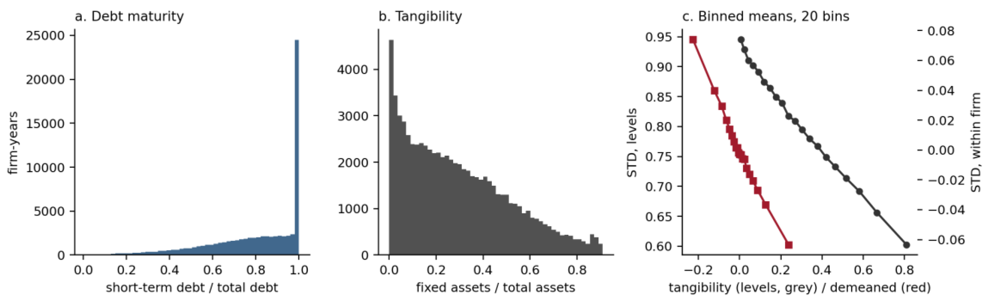
The right-hand panel answers a question the coefficient alone cannot. Both curves are close to straight over the whole support, so the linear form is not concealing a threshold, and the within relationship is not an artefact of the mass point at unity: it is present across the interior of the distribution as well. The specification with a squared term in Appendix B confirms this formally, and the specification that drops all observations at the two bounds returns a larger coefficient, not a smaller one.
Table A4.
Measurement validation, two independent constructions.
| Construct | Primary construction | Alternative construction | Corr. | β, primary | β, alternative |
|---|---|---|---|---|---|
| Short-term share | Filed maturity index | 1—long-term debt / total debt, from the financial coverage identity | 0.984 | −0.2410*** (0.0102) | −0.2165*** (0.0095) |
| Tangibility | Fixed assets / total assets | Fixed assets weighted by the tangible share of amortisation | 0.666 | −0.2410*** (0.0102) | −0.2124*** (0.0129) |
Note. Dependent variable: short-term debt over total debt. Coefficients on tangibility from the two-way fixed-effects specification of Table 3 with the stated variable substituted; standard errors clustered at firm level in parentheses. *** p < 0.01, ** p < 0.05, * p < 0.10. The alternative short-term share is obtained by recovering long-term debt as the financial coverage ratio multiplied by fixed assets, minus net worth, and dividing by total debt; it shares no balance-sheet item with the filed maturity index beyond net worth. The alternative tangibility measure apportions fixed assets by the observed mix of tangible and intangible amortisation, a flow proxy for a stock, which is why its correlation with the primary measure is lower. The alternative specifications are estimated on 73,113 and 70,850 firm-years respectively, since neither alternative is recoverable for every account.
The first row is a genuine check and it passes: two routes through the balance sheet, sharing no common item beyond net worth, give the same variable to within two per cent of its variance and the same coefficient to within two-tenths of a standard error. The second row is weaker by design. AIDA does not disaggregate fixed assets into tangible, intangible and financial, so the alternative apportions them by the observed mix of tangible and intangible amortisation. That mix is a flow proxy for a stock and the correlation of 0.666 reflects it. The coefficient is nonetheless unchanged, which is the relevant point: what the estimate captures is not the intangible component masquerading as tangibility.
Appendix B. The Panel Estimates in Full
Table B1.
Specification tests.
| Test | Null hypothesis | Statistic | Distribution | p |
|---|---|---|---|---|
| F on joint significance of firm effects | No individual effects (pooled OLS is adequate) | 9.31*** | F(11,264; 62,393) | < 0.001 |
| Breusch–Pagan Lagrange multiplier | No variance in the individual effects | 65,218.57*** | χ²(1) | < 0.001 |
| Hausman, fixed against random effects | Effects uncorrelated with the regressors | 313.96*** | χ²(4) | < 0.001 |
| Wooldridge AR(1) in the within residuals | No first-order serial correlation | ρ = 0.272*** | t (39.33) | < 0.001 |
Note. All tests are computed on the estimation sample of 73,662 firm-year observations and 11,265 firms. *** p < 0.01, ** p < 0.05, * p < 0.10. The first three tests reject pooled OLS and random effects in turn, which is why two-way fixed effects is the reference specification of Table 3. The fourth test rejects the absence of serial correlation, which is why all standard errors reported in the article are clustered at firm level, and why the static specification is complemented by the dynamic estimates of Table B5.
The three poolability tests agree, which is not always the case, and the reason they agree is visible in Table A3: firm heterogeneity accounts for more of the variance in maturity structure than time does. The fourth line is the qualification. Within residuals are serially correlated at 0.272, so the fixed-effects standard errors would be understated if they were not clustered at firm level; they are, throughout. Serial correlation of this magnitude is also the reason the static specification is not the last word, which is taken up below.
Table B2.
Twenty-nine specifications.
| Specification | β (TANG) | SE | Obs. | Firms | R² within |
|---|---|---|---|---|---|
| S1 Tangibility alone | −0.2814*** | (0.0106) | 73,662 | 11,265 | 0.055 |
| S2 + size | −0.2600*** | (0.0103) | 73,662 | 11,265 | 0.081 |
| S3 + size, coverage | −0.2438*** | (0.0102) | 73,662 | 11,265 | 0.092 |
| S4 Baseline: + size, coverage, growth | −0.2410*** | (0.0102) | 73,662 | 11,265 | 0.092 |
| S5 + leverage | −0.2474*** | (0.0100) | 73,662 | 11,265 | 0.122 |
| S6 + liquidity | −0.3648*** | (0.0105) | 73,662 | 11,265 | 0.189 |
| S7 + capital turnover | −0.2162*** | (0.0101) | 73,662 | 11,265 | 0.110 |
| S8 + profitability | −0.2400*** | (0.0103) | 73,662 | 11,265 | 0.093 |
| S9 Full control set | −0.4520*** | (0.0100) | 73,662 | 11,265 | 0.333 |
| S10 + squared tangibility | −0.2690*** | (0.0238) | 73,662 | 11,265 | 0.093 |
| S11 Dependent variable from the coverage identity | −0.2165*** | (0.0095) | 73,113 | 11,207 | 0.086 |
| S12 Regressor: tangible-only fixed assets | −0.2124*** | (0.0129) | 70,850 | 11,110 | 0.074 |
| S13 Firm effects only | −0.2470*** | (0.0094) | 73,662 | 11,265 | 0.093 |
| S14 Asset-weighted | −0.3008*** | (0.0257) | 73,662 | 11,265 | 0.104 |
| S15 Revenue-weighted | −0.3081*** | (0.0176) | 73,662 | 11,265 | 0.122 |
| S16 Innovative start-ups | −0.1205*** | (0.0287) | 6,535 | 2,213 | 0.036 |
| S17 Innovative SMEs | −0.1766*** | (0.0173) | 18,629 | 2,763 | 0.069 |
| S18 Ordinary SMEs | −0.3122*** | (0.0137) | 48,498 | 6,289 | 0.128 |
| S19 Certified firms only | −0.1633*** | (0.0151) | 25,164 | 4,976 | 0.063 |
| S20 Excluding 2020 and 2021 | −0.2640*** | (0.0115) | 56,835 | 11,239 | 0.106 |
| S21 Firms observed at least five years | −0.2569*** | (0.0109) | 64,843 | 8,086 | 0.103 |
| S22 Leverage above median | −0.2669*** | (0.0157) | 36,831 | 7,942 | 0.087 |
| S23 Leverage below median | −0.2146*** | (0.0147) | 36,831 | 7,864 | 0.092 |
| S24 Size above median | −0.3047*** | (0.0163) | 36,831 | 5,417 | 0.117 |
| S25 Size below median | −0.1917*** | (0.0137) | 36,831 | 7,524 | 0.067 |
| S26 Positive EBITDA only | −0.2313*** | (0.0107) | 65,706 | 10,752 | 0.126 |
| S27 Tangibility trimmed at 2 and 98 per cent | −0.2460*** | (0.0104) | 70,714 | 11,062 | 0.093 |
| S28 Dropping the bounds of the dependent variable | −0.2743*** | (0.0130) | 49,188 | 8,704 | 0.070 |
| S29 Excluding firms with no financial charges | −0.2809*** | (0.0122) | 57,180 | 9,300 | 0.096 |
Note. Dependent variable: short-term debt over total debt. Each row is a separate regression of the short-term share on tangibility and the stated controls. All specifications are two-way fixed effects with standard errors clustered at firm level, reported in parentheses, except S13, which carries firm effects only. *** p < 0.01, ** p < 0.05, * p < 0.10. The smallest test statistic in the grid is S16 at t = 4.20, so every coefficient clears the one per cent level. S4 is the baseline reported in Table 3. A northern-regions split was attempted and is not reported, because the regional field is available only for the certified populations.
Figure B1.
The coefficient on tangibility across the thirty specifications. Note. Point estimates with ninety-five per cent intervals; the dashed line marks the baseline of S4.
Figure B1.
The coefficient on tangibility across the thirty specifications. Note. Point estimates with ninety-five per cent intervals; the dashed line marks the baseline of S4.
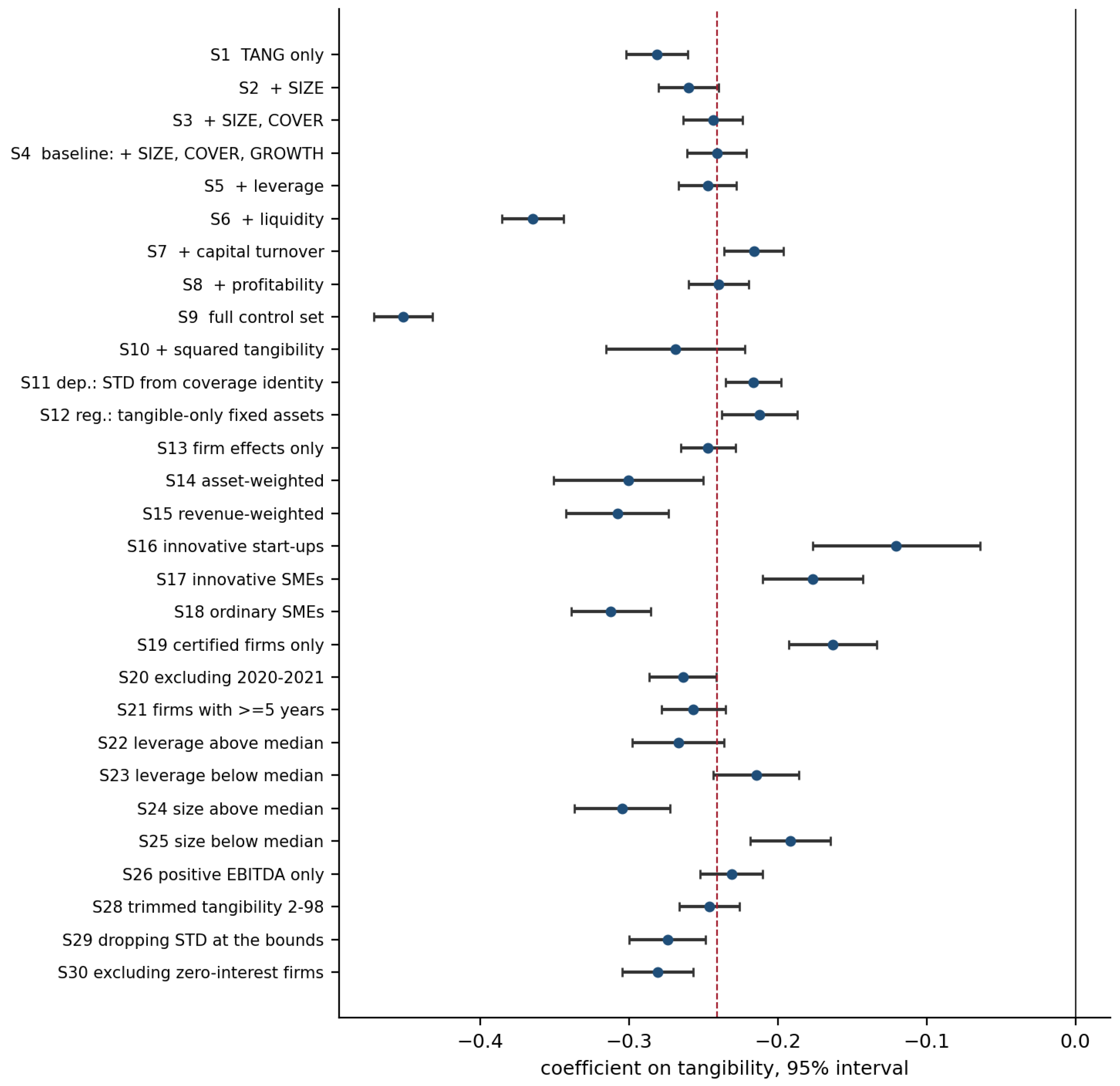
The interval spanned by the grid is −0.121 to −0.452, and it never touches zero. Three of the movements inside it are worth naming. Adding liquidity (S6) pushes the coefficient to −0.365 because liquid assets are the mirror image of fixed ones in the balance-sheet identity, so conditioning on liquidity isolates the part of tangibility that is not simply the absence of cash. Adding capital turnover (S7) pulls it to −0.216 for the opposite reason: turnover is itself a function of the asset base and absorbs part of the same variation. The full control set (S9) doubles the within R² to 0.333 and takes the coefficient to −0.452, which shows that the baseline is if anything conservative. What none of the movements do is threaten the sign, and the two sample cuts that most plausibly could have—dropping the mass point at the upper bound (S29), and dropping the pandemic years (S20)—both move the estimate away from zero.
Table B3.
Slope differences across the three regulatory regimes.
| Coefficient | SE | p | |
|---|---|---|---|
| TANG (ordinary SMEs, reference) | −0.3151*** | (0.0141) | < 0.001 |
| TANG × innovative SME | 0.1364*** | (0.0221) | < 0.001 |
| TANG × innovative start-up | 0.1966*** | (0.0295) | < 0.001 |
| SIZE | −0.0433*** | (0.0025) | < 0.001 |
| COVER | 0.0067*** | (0.0004) | < 0.001 |
| GROWTH | 0.0113*** | (0.0015) | < 0.001 |
| Implied slope, innovative SMEs | −0.1787 | ||
| Implied slope, innovative start-ups | −0.1185 | ||
| Observations | 73,662 | ||
| Firms | 11,265 |
Note. Dependent variable: short-term debt over total debt. A single two-way fixed-effects equation estimated on the pooled sample with regime interactions; standard errors clustered at firm level in parentheses. *** p < 0.01, ** p < 0.05, * p < 0.10. The regime main effects are absorbed by the firm effects, since regulatory status does not vary within a firm over the sample period. The interaction terms are positive because both certified regimes match maturities less strongly than the ordinary-SME reference; the implied slopes in italics are the sum of the reference coefficient and the corresponding interaction, and correspond to the separate-sample estimates S17 and S16 of Table B2.
Table B4.
The cross-sectional coefficient year by year.
| Year | β (TANG) | SE | Firm-years |
|---|---|---|---|
| 2016 | −0.3998*** | (0.0151) | 4,770 |
| 2017 | −0.4075*** | (0.0126) | 6,921 |
| 2018 | −0.4055*** | (0.0126) | 7,322 |
| 2019 | −0.3913*** | (0.0122) | 7,762 |
| 2020 | −0.3736*** | (0.0124) | 8,140 |
| 2021 | −0.3906*** | (0.0119) | 8,687 |
| 2022 | −0.3561*** | (0.0111) | 9,509 |
| 2023 | −0.3580*** | (0.0102) | 10,399 |
| 2024 | −0.3475*** | (0.0101) | 10,152 |
| Change, 2016 to 2024 | 0.0523*** | (0.0182) |
Note. Dependent variable: short-term debt over total debt. Each row is a separate cross-sectional regression on the firms observed in that year, with the controls of Table 3 and standard errors clustered at firm level, reported in parentheses. *** p < 0.01, ** p < 0.05, * p < 0.10. These are cross-sectional estimates and therefore inherit the composition that the fixed-effects estimator removes; their interest lies in the trend rather than in the level. The final row tests the difference between the first and last year, treating the two estimates as independent. The weakening is monotone apart from 2021, and coincides with a decade of falling long-term rates and expanding public guarantee coverage.
Figure B2.
Time profile and regime heterogeneity. Note. Left: the year-by-year cross-sectional coefficient with ninety-five per cent intervals. Right: the within-firm coefficient estimated separately on the three regulatory populations, in absolute value.
Figure B2.
Time profile and regime heterogeneity. Note. Left: the year-by-year cross-sectional coefficient with ninety-five per cent intervals. Right: the within-firm coefficient estimated separately on the three regulatory populations, in absolute value.
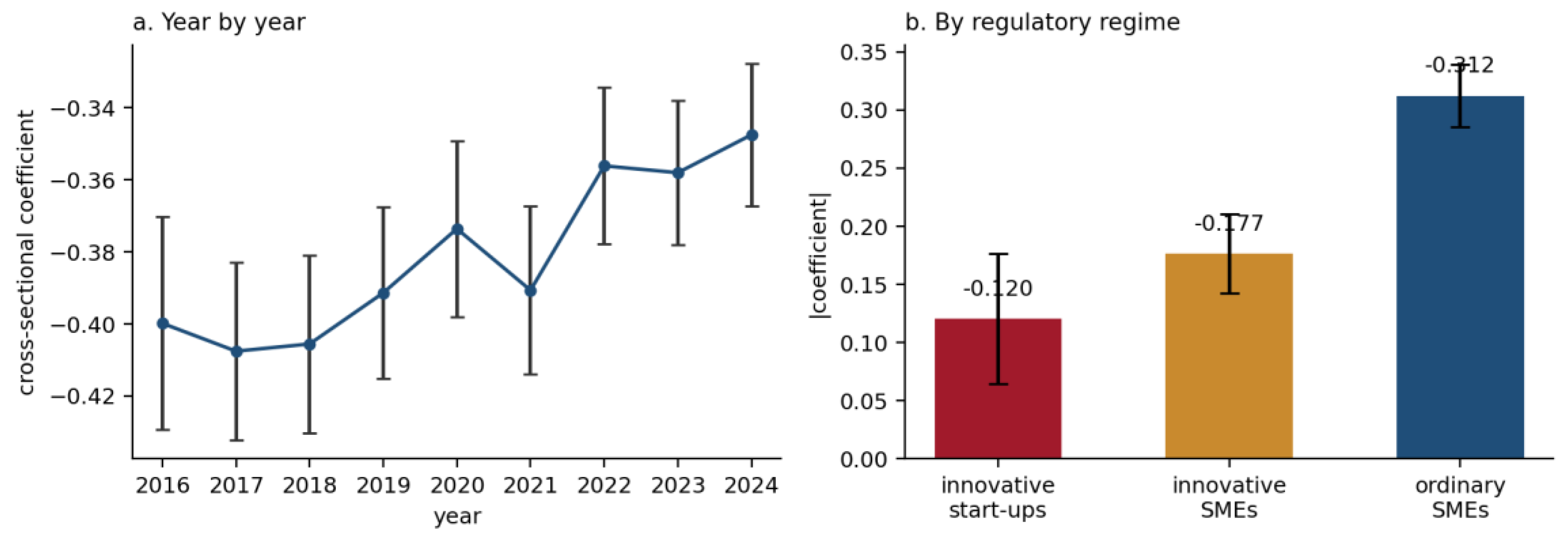
The two panels report different things and it is worth saying which. The left panel is a cross-section repeated nine times, so it inherits the composition that the fixed-effects estimator removes; its interest is the trend, a monotone weakening from −0.400 to −0.348 across a decade of falling long-term rates and expanding public guarantee coverage. The right panel is nine years of within-firm variation split three ways, and the gradient is steep: ordinary SMEs match maturities at −0.312, innovative SMEs at −0.177, innovative start-ups at −0.120, with both differences from the reference significant at one per cent in the pooled interaction of Table B3. Maturity matching is something a firm does when it can choose its maturity structure. A certified innovative firm whose assets are largely uncollateralisable, and whose bank credit arrives predominantly through short-horizon guaranteed lines, has less of a choice to make, and the flatter slope is what that constraint looks like in the data.
Table B5.
Dynamic specifications.
| Estimator | ρ | β (TANG) | Long-run β | F | J (p) | Obs. |
|---|---|---|---|---|---|---|
| Two-way FE with lagged dep. var. (lower bound) | 0.3173*** (0.0078) | −0.1900*** (0.0104) | −0.2783 | — | — | 61,485 |
| Pooled OLS with lagged dep. var. (upper bound) | 0.7210*** (0.0042) | −0.1158*** (0.0036) | −0.4152 | — | — | 61,485 |
| Anderson–Hsiao, FD, STD(t−2) | 0.5558*** (0.0144) | −0.1940*** (0.0139) | −0.4367 | 3,434.9 | — | 49,949 |
| Anderson–Hsiao, FD, STD(t−2), STD(t−3) | 0.5660*** (0.0182) | −0.2202*** (0.0158) | −0.5074 | 3,554.8 | 38.43 (0.000) | 40,063 |
Note. Dependent variable: short-term debt over total debt. Standard errors clustered at firm level in parentheses. *** p < 0.01, ** p < 0.05, * p < 0.10. ρ is the coefficient on the lagged dependent variable and the long-run coefficient is β / (1—ρ). F is the first-stage statistic on the instrumented lagged difference; J is the Hansen overidentification statistic, computable only where the instruments outnumber the endogenous regressor. The first two rows bound ρ from below and above, since the fixed-effects estimator is biased downwards and pooled OLS upwards in the presence of a lagged dependent variable. The Anderson–Hsiao estimate of 0.556 falls inside that interval. The overidentified variant is rejected by its Hansen test, which is expected given the AR(1) documented in Table B1, so the just-identified row is the one to read; its long-run coefficient of −0.437 is 1.8 times the static estimate of Table 3.
Figure B3.
Persistence and the accumulated response. Note. Left: the estimated persistence of debt maturity under four estimators; the shaded band is the interval defined by the two estimators whose bias is signed. Right: short-run and accumulated coefficients on tangibility.
Figure B3.
Persistence and the accumulated response. Note. Left: the estimated persistence of debt maturity under four estimators; the shaded band is the interval defined by the two estimators whose bias is signed. Right: short-run and accumulated coefficients on tangibility.
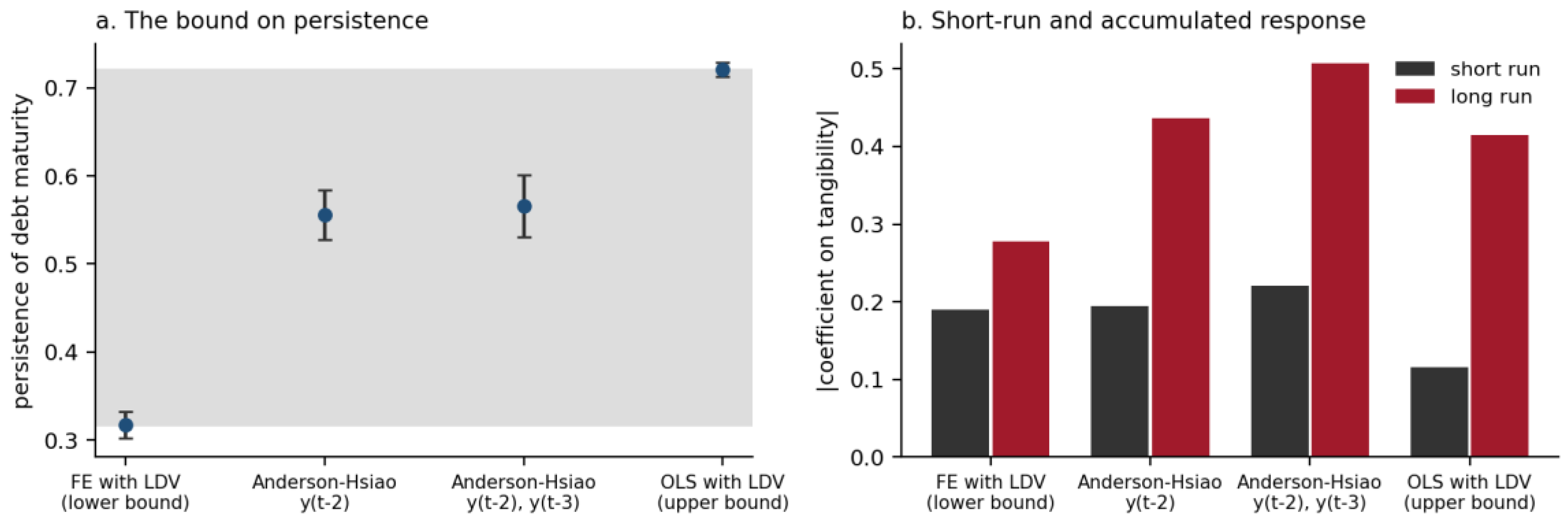
The minimal credibility check for a dynamic panel is that the instrumented estimate falls inside the bracket formed by the two biased ones, and it does: 0.556 lies between the fixed-effects lower bound of 0.317 and the pooled upper bound of 0.721. Debt maturity is therefore substantially persistent—a little over half of last year’s composition survives into this year—and the static coefficient of Table 3 understates the eventual response by a factor of about 1.8. The overidentified variant fails its Hansen test, which is expected given the AR(1) in the residuals documented in Table B1, so the just-identified estimate is the one to read; the accumulated coefficient of −0.437 is the appropriate magnitude for any horizon longer than a year.
Table B6.
The baseline coefficient under alternative inference.
| Standard errors | SE (TANG) | t | 95% interval | Clusters | df |
|---|---|---|---|---|---|
| Firm (baseline) | 0.0102 | −23.61 | [−0.261, −0.221] | 11,265 | 11,264 |
| Year only | 0.0189 | −12.74 | [−0.285, −0.197] | 9 | 8 |
| Two-way, firm and year | 0.0204 | −11.82 | [−0.288, −0.194] | 9 | 8 |
| Driscoll–Kraay, Bartlett lag 2 | 0.0242 | −9.97 | [−0.297, −0.185] | 9 | 8 |
| Firm block bootstrap, 300 replications | 0.0089 | −26.97 | [−0.259, −0.224] | 11,265 | 11,264 |
Note. Dependent variable: short-term debt over total debt. All rows report the same two-way fixed-effects point estimate of −0.2410 from Table 3; only the variance estimator changes. Two-way clustering follows Cameron, Gelbach and Miller, adding the firm-clustered and year-clustered matrices and subtracting the intersection; a negative-eigenvalue correction was not required. Inference on the rows with nine year clusters uses the t distribution with eight degrees of freedom, whose two-sided five per cent critical value is 2.306. Driscoll–Kraay allows for cross-sectional dependence with a Bartlett kernel truncated at two lags. The block bootstrap resamples firms with replacement.
Clustering at firm level is the convention in this literature, but it assumes that shocks are independent across firms within a year, which a common credit cycle would violate. Allowing for that dependence doubles the standard error on tangibility, from 0.0102 to 0.0204, and the Driscoll–Kraay estimator, which additionally permits cross-sectional dependence to decay over time, raises it to 0.0242. Neither comes close to overturning the result: the t statistic falls from 23.6 to between 10 and 12, against a critical value of 2.306 on the eight degrees of freedom that nine year clusters allow. The confidence interval widens from [−0.261, −0.221] to [−0.297, −0.185], which still excludes zero by a wide margin and still excludes the between estimate of −0.380.
Two caveats attach to the last three rows. Nine clusters is few, and cluster-robust inference is known to be unreliable in that range even with the small-sample degrees-of-freedom correction applied here; the year-clustered standard errors should be read as indicative rather than exact. And the widening is what a common time-varying factor would produce, but it is also what any nine-group aggregation produces mechanically, so it is evidence that the result is robust to the assumption rather than evidence about the assumption itself. The firm block bootstrap, which relaxes the parametric form of the firm-level dependence without reducing the number of clusters, returns a standard error of 0.0089, slightly tighter than the analytical firm-clustered figure—which suggests the baseline is if anything conservative in the dimension where the data support inference.
Firm-level clustering is retained throughout the article because the number of year clusters is too small to support it as the default, and because the choice is the more conservative of the two dimensions in which the sample is large.
Appendix C. Instrumental Variables
Tangibility is not randomly assigned. A firm that has secured a ten-year loan may buy the machine the loan was granted against, which reverses the direction of the association; and book fixed assets are measured with error, because they depend on depreciation policy and on the age of the asset stock rather than on its economic value alone. The two problems push in opposite directions, so the sign of the bias in Table 3 is not known a priori, and instrumentation is worth attempting even if it cannot be expected to identify the parameter.
Four instrument families were tried. The first is internal: the second and third lags of tangibility, applied to the first-differenced equation in the manner of Anderson and Hsiao, valid if the differenced error is not correlated at those horizons. The second is the accumulated depreciation ratio, which shifts book tangibility mechanically through the age of the asset stock. The third and fourth are leave-one-out peer means of tangibility, computed at province × year and at sector × year, which would capture technological shocks to asset composition common to a firm’s neighbours but external to its own financing decision.
Table C1.
Instrumental-variable estimates, first-differenced equation.
| Instrument set | β | Obs. | F | Partial R² | J (p) | WuH p |
|---|---|---|---|---|---|---|
| Panel A. Internal instruments and the depreciation ratio | ||||||
| TANG(t−2) | −0.332*** (0.035) | 49,949 | 1,170.2 | 0.024 | — | 0.003 |
| TANG(t−2), TANG(t−3) | −0.398*** (0.044) | 40,063 | 979.4 | 0.023 | 1.25 (0.263) | 0.001 |
| Accumulated depreciation ratio | −0.423*** (0.063) | 17,017 | 305.4 | 0.025 | — | 0.000 |
| TANG(t−2) and depreciation ratio | −0.435*** (0.050) | 13,704 | 580.2 | 0.052 | 0.07 (0.788) | 0.000 |
| TANG(t−2), TANG(t−3), depreciation | −0.480*** (0.058) | 10,608 | 455.8 | 0.054 | 0.38 (0.827) | 0.000 |
| Panel B. Peer instruments (reported as failures) | ||||||
| Peer mean, province × year | −2.093*** (0.278) | 61,328 | 71.8 | 0.002 | — | 0.000 |
| Peer mean, sector × year | −4.610 (3.689) | 18,680 | 1.6 | 0.000 | — | 0.000 |
| Peer mean, sector × province × year | 117.98 (4,875.9) | 10,391 | 0.001 | 0.000 | — | 0.035 |
| TANG(t−2) and peer mean, province × year | −0.483*** (0.036) | 49,828 | 1,268.8 | 0.027 | 145.46 (0.000) | 0.000 |
| Panel C. Uninstrumented benchmarks | ||||||
| First-differenced OLS, t−2 sample | −0.211*** (0.011) | 49,949 | — | — | — | — |
| First-differenced OLS, t−3 sample | −0.236*** (0.013) | 40,063 | — | — | — | — |
| First-differenced OLS, full sample | −0.200*** (0.010) | 61,485 | — | — | — | — |
Note. Dependent variable: the first difference of the short-term share of debt. All equations are estimated in first differences with the differenced controls of Table 3 and standard errors clustered at firm level, reported in parentheses. *** p < 0.01, ** p < 0.05, * p < 0.10. F is the first-stage statistic, Partial R² the incremental explanatory power of the excluded instruments, J the Hansen overidentification statistic and WuH the Wu–Hausman test of the exogeneity of tangibility. Panel C reports the uninstrumented benchmarks on the corresponding samples. Statistical significance is not by itself evidence that an instrument is usable: the province-level peer mean in Panel B has a first-stage F of 71.8 and a coefficient significant at one per cent, yet a partial R² of 0.002 and a point estimate of −2.09 that lies outside the admissible range for a share, and its combination with a lag is rejected by Hansen at p < 0.001. The three peer specifications are therefore reported as failures rather than as results, and Panel A carries the corroborative evidence.
Figure C1.
Instrument strength and the resulting estimates. Note. Left: point estimates with ninety-five per cent intervals; the axis is truncated at −1.2 and the dashed line marks the two-way fixed-effects benchmark of Table 3. Right: first-stage F statistics on a logarithmic scale, with the conventional threshold at 10; grey bars fall below it.
Figure C1.
Instrument strength and the resulting estimates. Note. Left: point estimates with ninety-five per cent intervals; the axis is truncated at −1.2 and the dashed line marks the two-way fixed-effects benchmark of Table 3. Right: first-stage F statistics on a logarithmic scale, with the conventional threshold at 10; grey bars fall below it.
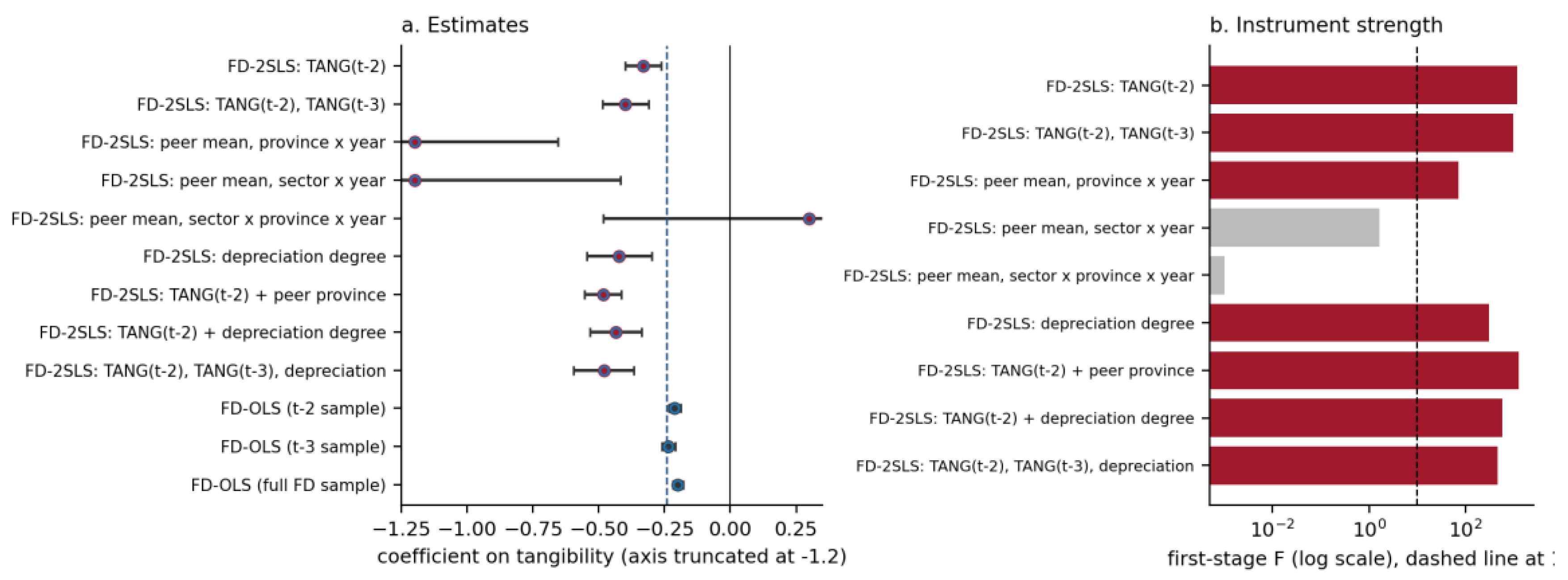
The two halves of the table should be read as one success and one failure, and both are reported because the failure is informative. The internal instruments are strong by any standard—first-stage F between 456 and 3,555, far above the conventional threshold—and the overidentification tests pass comfortably wherever the instruments are numerous enough to compute them, at p = 0.263 for the two lags and p = 0.827 when the depreciation ratio is added. Their point estimates run from −0.332 to −0.480 against a first-differenced least-squares benchmark of −0.211 on the identical sample. That is the pattern classical measurement error produces: differencing amplifies noise relative to signal, least squares is attenuated towards zero, and instrumenting with a lag that shares the signal but not the noise restores the magnitude. The Wu–Hausman test rejects exogeneity at one per cent throughout, so the difference between the two columns is not sampling variation.
The peer instruments fail, and they fail in the way weak instruments always do. The province-level mean has a first-stage F of 71.8, which passes the rule of thumb, but a partial R² of 0.002 and an implied coefficient of −2.09—six standard deviations from every other estimate in this appendix and outside the admissible range for a share. The sector-level means have F statistics of 1.6 and 0.001 and produce estimates with no information in them at all. The combination of a lag with the province mean is rejected by Hansen at p < 0.001, which says the two instruments are not estimating the same parameter. The conclusion is the one the previous paper in this series reached about a different regressor: the supply-side variation that would identify the coefficient is not correlated strongly enough with the firm-level regressor to be usable in these data, and the internal instruments corroborate the fixed-effects estimate without upgrading its status from association to cause.
Table C2.
Firm age as an additional control, certified populations.
| Specification | β (TANG) | β (ln age) | Obs. | Firms | R² within |
|---|---|---|---|---|---|
| Certified subsample, baseline controls | −0.1659*** (0.0156) | — | 22,938 | 4,610 | 0.063 |
| Certified subsample, adding ln age | −0.1670*** (0.0156) | −0.0336*** (0.0104) | 22,938 | 4,610 | 0.064 |
Note. Dependent variable: short-term debt over total debt. Two-way fixed-effects estimates with the controls of Table 3 and standard errors clustered at firm level, reported in parentheses. *** p < 0.01, ** p < 0.05, * p < 0.10. Firm age is the difference between the accounting year and the year of entry in the Business Register, matched on fiscal code from the registers of innovative start-ups and innovative SMEs; the register is not available for the ordinary SME comparison group, so the control can be applied to 31.1 per cent of the estimation sample only. Adding age moves the coefficient on tangibility by 0.0011, less than a tenth of its standard error, which is why age is omitted from the baseline specification without cost: it is time-varying but nearly collinear with the year effects inside a nine-year window.
The reason age is confined to the appendix is the coverage constraint in the note, not a judgement about its relevance. Where it can be measured it behaves as expected—older firms hold slightly less short-term debt, at one per cent significance—and it is close to irrelevant for the question at hand: adding it moves the coefficient on tangibility from −0.1659 to −0.1670, a shift of less than a tenth of a standard error. Since firm age is time-varying but almost collinear with the year effects inside a nine-year window, this is what should have been expected, and it means the omission of age from the main specification costs nothing.
Appendix D. Design of the Clustering Exercise
Three design choices precede any algorithm, and each of them can change the answer more than the choice of algorithm does.
The first is the unit. Clustering firm-years would have produced a partition in which the same firm migrates between groups as its accounts fluctuate, which is a description of annual states rather than of firms. Firm averages over the nine years were used instead, so the taxonomy is a property of the firm and can be carried back into a panel equation without generating a mechanical correlation between cluster membership and the year-to-year variation the fixed-effects estimator uses.
The second is the dimension set. The nine dimensions are exactly the nine analysis variables of the panel module, standardised. Including the dependent variable is deliberate: excluding it would build a taxonomy of the right-hand side and then discover that it explains the left-hand side, which is not informative. Including it with a weight of one ninth means the partition is not driven by it—and Table 3 confirms this, since three of the five clusters have almost identical short-term shares of 0.88 to 0.89 and are separated by everything else.
The third is the number of clusters.
Table D1.
Choosing the number of clusters, K-means reference.
| k | R² | AIC | BIC | Silhouette | Calinski–Harabasz | Dunn | Entropy | HHI |
|---|---|---|---|---|---|---|---|---|
| 2 | 0.174 | 268,431 | 268,570 | 0.200 | 1,064 | 0.028 | 0.924 | 0.552 |
| 3 | 0.280 | 254,513 | 254,719 | 0.175 | 971 | 0.024 | 0.942 | 0.379 |
| 4 | 0.366 | 241,641 | 241,912 | 0.166 | 972 | 0.022 | 0.944 | 0.285 |
| 5 | 0.418 | 232,925 | 233,262 | 0.166 | 905 | 0.021 | 0.957 | 0.227 |
| 6 | 0.455 | 226,252 | 226,655 | 0.150 | 842 | 0.034 | 0.961 | 0.191 |
| 7 | 0.486 | 220,359 | 220,828 | 0.148 | 795 | 0.028 | 0.966 | 0.163 |
| 8 | 0.509 | 215,694 | 216,229 | 0.145 | 748 | 0.028 | 0.965 | 0.144 |
| 9 | 0.529 | 211,587 | 212,188 | 0.148 | 710 | 0.033 | 0.961 | 0.132 |
| 10 | 0.545 | 208,050 | 208,717 | 0.151 | 676 | 0.028 | 0.951 | 0.125 |
Figure D1.
The scan over the number of clusters. Note. Left: variance explained. Centre: Bayesian information criterion. Right: silhouette against the entropy of cluster sizes; the dashed line marks the chosen solution.
Figure D1.
The scan over the number of clusters. Note. Left: variance explained. Centre: Bayesian information criterion. Right: silhouette against the entropy of cluster sizes; the dashed line marks the chosen solution.
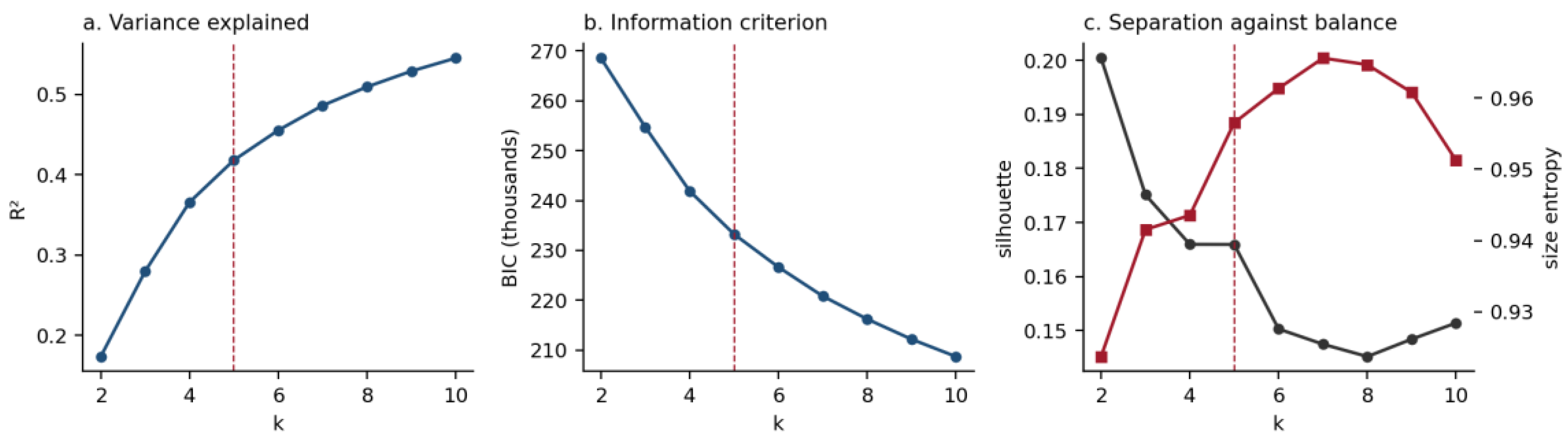
The three panels disagree, and it is worth saying so plainly rather than presenting a consensus that does not exist. Variance explained rises monotonically and has no elbow; the information criteria fall monotonically to k = 10 and would keep falling; the silhouette is maximised at two clusters, which is the value it almost always takes on continuous data because two well-separated halves beat any finer division on average nearest-neighbour distance. Only the entropy of the size distribution has an interior maximum, at seven. Five was chosen as the smallest number at which the entropy exceeds 0.95 and the Herfindahl falls below 0.23—that is, the smallest partition in which no cluster dominates—and the same k was imposed on every algorithm so that Table 5 compares methods rather than granularities. Nothing in the substantive results turns on it: at k = 4 and k = 6 the ordering of the cluster-level maturity coefficients is unchanged.
Appendix E. Algorithm Settings and the Two Tuned Families
Four of the six families have no tuning parameter beyond k. Two do, and both were scanned.
Table E1.
Fuzzy C-means, the fuzzifier.
| m | Effective clusters | Partition coefficient | Partition entropy |
|---|---|---|---|
| 1.3 | 5 | 0.665 | 0.644 |
| 1.5 | 5 | 0.463 | 1.066 |
| 2.0 | 3 | 0.200 | 1.609 |
| 2.5 | 5 | 0.200 | 1.609 |
Note. Effective clusters counts the distinct labels after defuzzification. A partition coefficient of 1/c = 0.200 indicates complete fuzziness, in which every firm belongs equally to every cluster.
The fuzzifier matters more than the literature usually admits. At the conventional default of m = 2 the algorithm collapses on these data: the partition coefficient reaches its theoretical minimum of 0.200 and defuzzification recovers only three distinct labels, because in nine standardised dimensions the distances between centroids are small relative to the spread and a quadratic fuzzifier flattens every membership towards 1/c. At m = 1.5 the solution is crisp enough to be a partition and fuzzy enough to record where the boundaries are, and that is the value used throughout.
Table E2.
Density-based clustering, the parameter grid.
| Method | Parameter | Clusters found | Firms assigned |
|---|---|---|---|
| HDBSCAN | min_cluster_size = 500, min_samples = 25 | 0 | 0.0% |
| HDBSCAN | min_cluster_size = 250, min_samples = 25 | 0 | 0.0% |
| HDBSCAN | min_cluster_size = 100, min_samples = 5 | 0 | 0.0% |
| HDBSCAN | min_cluster_size = 100, min_samples = 1 | 2 | 26.0% |
| HDBSCAN | min_cluster_size = 50, min_samples = 1 | 2 | 26.0% |
| DBSCAN | ε = 1.021 (median 10-NN distance) | 2 | 64.1% |
| DBSCAN | ε = 1.368 (75th percentile) | 2 | 86.2% |
| DBSCAN | ε = 1.727 (90th percentile) | 1 | 96.1% |
| DBSCAN | ε = 1.998 (95th percentile) | 1 | 98.3% |
The grid documents a failure that is itself a finding. HDBSCAN, which selects clusters by excess of mass over a hierarchy of density levels, declares the entire sample noise at every setting with a minimum sample count above one: in nine standardised dimensions there is no density gap anywhere in these data, because balance-sheet configurations form a continuum rather than islands. DBSCAN can be forced to produce a partition, but only by moving along a trade-off in which the number of clusters and the share of firms classified move in opposite directions—two clusters and a third of the sample discarded, or one cluster and nothing learned. The configuration reported in Table 5 is the most favourable point on that curve, and it is still the worst solution in the set on every non-geometric criterion.
Figure E1.
Centroids and regulatory composition. Note. Left: cluster centroids in standard deviations from the sample mean on each of the nine dimensions. Right: the regulatory composition of each cluster; the regulatory label took no part in the estimation.
Figure E1.
Centroids and regulatory composition. Note. Left: cluster centroids in standard deviations from the sample mean on each of the nine dimensions. Right: the regulatory composition of each cluster; the regulatory label took no part in the estimation.
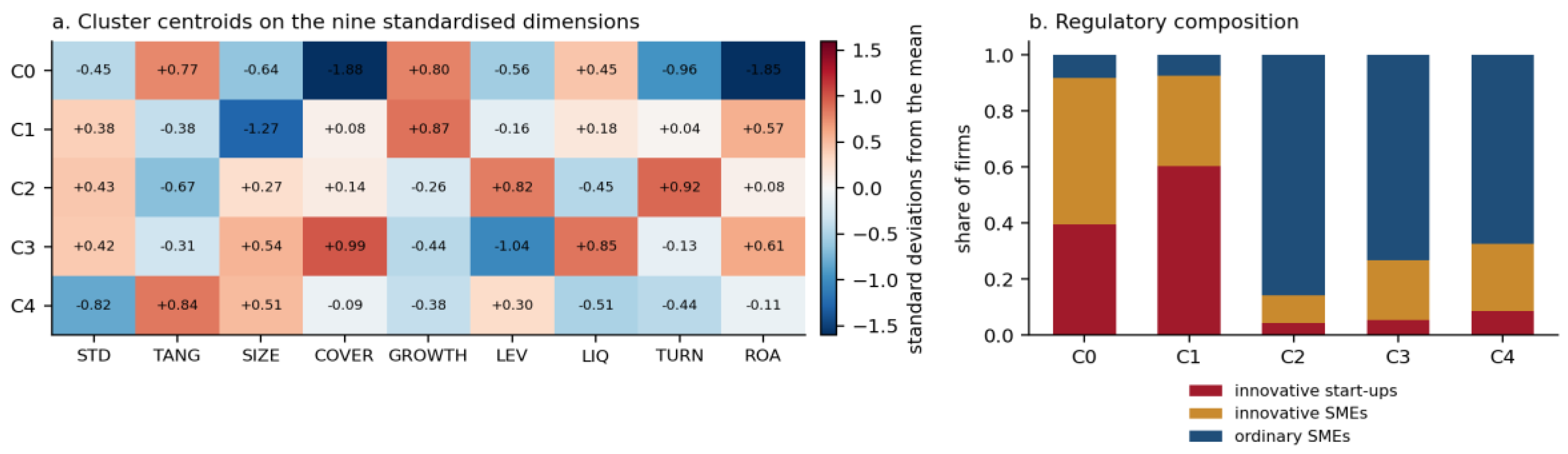
Table E3.
Regulatory composition of the five clusters.
| Cluster | Innovative start-ups | Innovative SMEs | Ordinary SMEs | Firms |
|---|---|---|---|---|
| C0 Loss-making asset builders | 39.5% | 52.4% | 8.1% | 1,293 |
| C1 Young and asset-light | 60.3% | 32.3% | 7.4% | 2,019 |
| C2 Levered traders | 4.3% | 9.8% | 85.9% | 2,942 |
| C3 Capitalised performers | 5.3% | 21.3% | 73.3% | 2,150 |
| C4 Capital-intensive | 8.5% | 24.0% | 67.5% | 2,861 |
The correspondence between an unsupervised partition and an administrative classification that played no part in producing it is strong but not perfect, and the imperfections are the interesting part. Two clusters are more than nine-tenths certified and two are more than two-thirds ordinary, so the algorithm has largely rediscovered the regulatory boundary from the accounts alone. But 8.1 per cent of C0 and 7.4 per cent of C1 are ordinary SMEs that look exactly like certified innovative firms on nine balance-sheet dimensions, and roughly a quarter of C3 and C4 are certified firms that look exactly like ordinary ones. The register does not partition the accounting space; it cuts across it.
Table E4.
Loadings on the two leading components.
| Dimension | PC1 | PC2 |
|---|---|---|
| Short-term share | 0.358 | 0.098 |
| Tangibility | −0.427 | −0.061 |
| ln total assets | 0.106 | −0.269 |
| Interest coverage | 0.502 | 0.078 |
| Revenue growth | −0.131 | 0.175 |
| Leverage | 0.024 | −0.621 |
| Liquidity | 0.026 | 0.633 |
| Capital turnover | 0.410 | −0.273 |
| Return on assets | 0.490 | 0.125 |
| Variance explained | 27.4% | 19.8% |
The first component is not a quality axis and not a size axis: size loads at 0.106 and the component is dominated by coverage, profitability, turnover and the negative of tangibility. It measures how intensively a firm turns a given asset base into revenue and profit, and the short-term share rides on it at 0.358. The second is a pure financial-structure axis, liquidity against leverage at 0.633 and −0.621, on which the maturity share loads at almost nothing. That the dependent variable of this study aligns with the operating axis and is orthogonal to the financing axis is a result in its own right, and it is consistent with the panel finding that maturity composition tracks asset composition rather than the level of debt.
Appendix F. The Equation Inside the Taxonomy
Table F1.
Pooled equation with cluster interactions.
| TANG (C0, reference) | −0.0863*** | (0.0284) | 0.002 |
|---|---|---|---|
| TANG × C1 | −0.0864** | (0.0363) | 0.017 |
| TANG × C2 | −0.1720*** | (0.0342) | < 0.001 |
| TANG × C3 | −0.1644*** | (0.0371) | < 0.001 |
| TANG × C4 | −0.2324*** | (0.0341) | < 0.001 |
| SIZE | −0.0434*** | (0.0024) | < 0.001 |
| COVER | 0.0067*** | (0.0004) | < 0.001 |
| GROWTH | 0.0109*** | (0.0015) | < 0.001 |
| Implied slope, C1 Young and asset-light | −0.1727 | ||
| Implied slope, C2 Levered traders | −0.2583 | ||
| Implied slope, C3 Capitalised performers | −0.2507 | ||
| Implied slope, C4 Capital-intensive | −0.3187 | ||
| Wald test, all interactions zero | 56.36*** | χ²(4) | < 0.001 |
| Observations | 73,662 | ||
| Firms | 11,265 |
Note. Dependent variable: short-term debt over total debt. A single two-way fixed-effects equation on the pooled sample with cluster interactions; standard errors clustered at firm level in parentheses. *** p < 0.01, ** p < 0.05, * p < 0.10. Cluster membership is the fuzzy C-means solution of Table 6, with C0 as the reference category. The cluster main effects are absorbed by the firm effects, since membership is assigned from firm averages and does not vary over time. The implied slopes in italics are the sum of the reference coefficient and the corresponding interaction; they differ slightly from the separate-sample estimates of Table 7 because this specification constrains the control coefficients to be common across clusters. Because the clusters were formed on dimensions that include both variables entering the equation, the interactions are descriptive rather than an out-of-sample test.
Figure F1.
Cluster-level coefficients and the fuzziness of the partition. Note. Left: the coefficient on tangibility estimated inside each cluster, in absolute value, with ninety-five per cent intervals; the dashed line is the whole-sample estimate. Right: the distribution of the maximum membership degree, with the 0.6 threshold marked.
Figure F1.
Cluster-level coefficients and the fuzziness of the partition. Note. Left: the coefficient on tangibility estimated inside each cluster, in absolute value, with ninety-five per cent intervals; the dashed line is the whole-sample estimate. Right: the distribution of the maximum membership degree, with the 0.6 threshold marked.
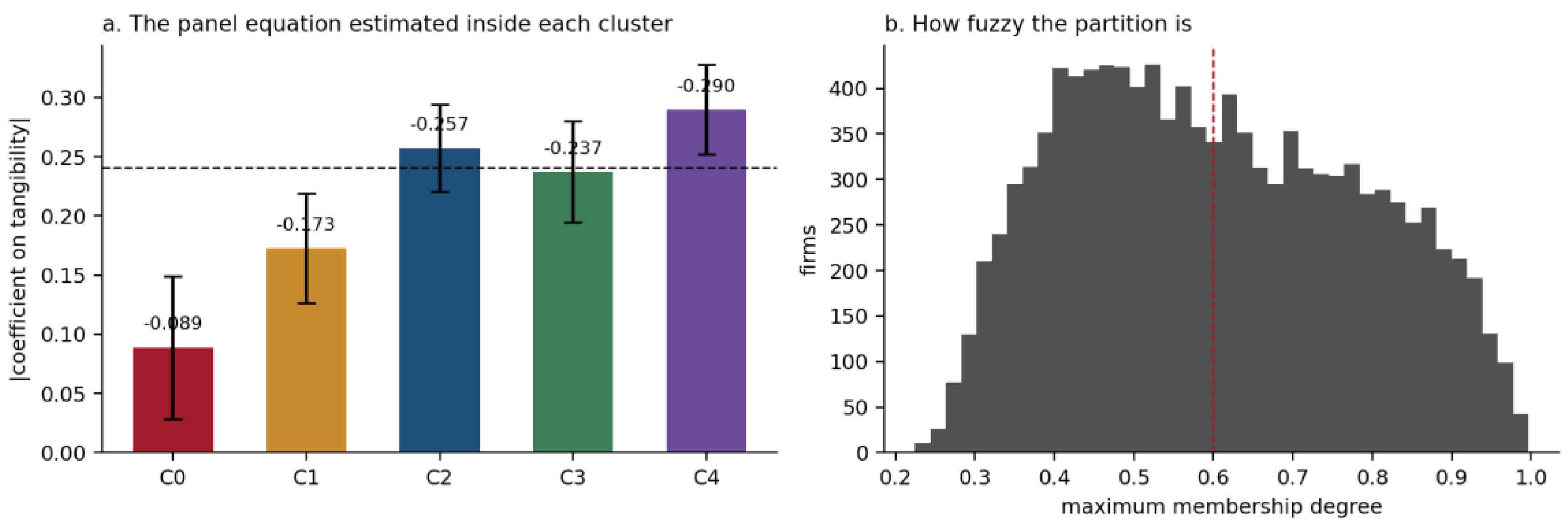
Two readings of the left panel should be kept apart. The clusters differ in their maturity-matching slope, and the difference is statistically decisive—but the clusters were formed on variables that include the slope’s own ingredients, so this is not an out-of-sample test of anything. What it is, is a demonstration that the heterogeneity found by the regime split of the panel module is recoverable from the accounts without the regime label, which makes it less likely that the regime result is an artefact of the certification process rather than of the balance sheets the certification selects on. The right panel is the caution attached to all of it: with a median maximum membership near 0.60, cluster assignment for the typical firm is a close call between two configurations, and the cluster-level coefficients should be read as describing regions of a continuum, not populations.
Appendix G. Stability
Figure G1.
Bootstrap stability of the five clusters. Note. Left: mean Jaccard similarity of each cluster with its best match across 25 bootstrap replications; the dashed line is the conventional 0.75 threshold for a stable cluster. Right: the adjusted Rand index of the whole partition against the reference solution.
Figure G1.
Bootstrap stability of the five clusters. Note. Left: mean Jaccard similarity of each cluster with its best match across 25 bootstrap replications; the dashed line is the conventional 0.75 threshold for a stable cluster. Right: the adjusted Rand index of the whole partition against the reference solution.
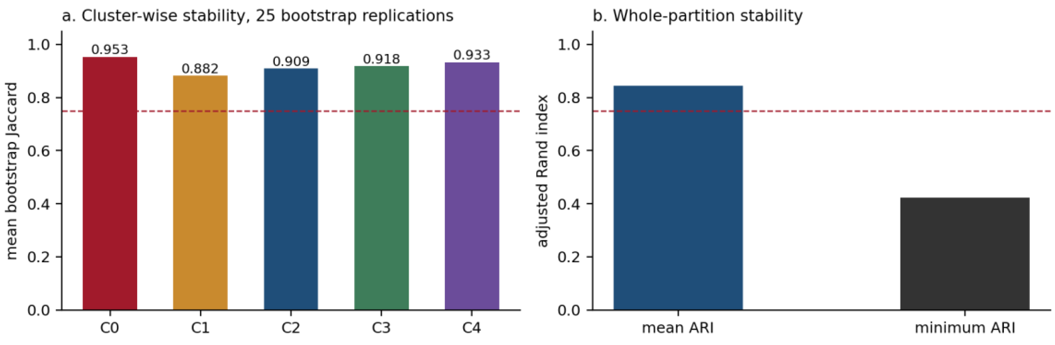
Each replication resamples the 11,265 firms with replacement, refits fuzzy C-means from a fresh random initialisation, and assigns every firm in the original sample to the nearest refitted centroid. All five clusters clear the conventional threshold comfortably, with mean Jaccard between 0.882 for C1 and 0.953 for C0. The whole-partition adjusted Rand index averages 0.845, with a standard deviation of 0.197 and a minimum of 0.423 across the 25 replications—the low tail arising in replications where two of the three ordinary-SME clusters exchange a boundary, which is the same softness the membership distribution records. The reading is that the five centres are a stable feature of these data and the walls between three of them are not sharp.
Appendix H. Machine Learning Regression for Validation
Table H1.
Learners and settings.
| Learner | Implementation | Settings |
|---|---|---|
| Linear regression | Ordinary least squares | no penalty |
| Linear SVM | Linear support-vector regression | C = 1.0, ε = 0.05, features standardised |
| K nearest neighbours | Distance-weighted KNN | k = 25, features standardised |
| Decision tree | CART, squared-error criterion | minimum 100 observations per leaf |
| Random forest | Bagged trees | 150 trees, minimum 50 per leaf, 80% of features |
| Gradient boosting | Histogram gradient boosting | 400 iterations, learning rate 0.06, 31 leaves |
The three data transformations are defined as follows. Levels uses the raw variables. Mundlak appends the firm mean of each regressor to the raw variables, which is the parametric device that makes a pooled regression reproduce the within estimator when the effects are linear. Within subtracts the firm mean and the year mean from every variable and adds back the grand mean, which is the two-way demeaning the fixed-effects estimator performs internally; the learner then works on exactly the variation the panel coefficients are identified from.
Cross-validation is grouped by firm rather than random. This matters here more than in a cross-section: with a mean of 6.5 observations per firm, a random split would place other years of the same firm in the training set, and any learner able to memorise a firm’s level would score on its own training information. The grouped design removes that channel, which is why the nearest-neighbour result in Table 9 collapses from an in-sample 1.000 to an out-of-sample 0.062 rather than to something respectable.
No hyperparameter search was run. The settings above are conventional defaults chosen before the results were seen, and they are deliberately conservative on capacity—minimum leaf sizes of 50 and 100 observations, a moderate learning rate, no boosting rounds beyond 400. A tuned learner would score higher, and the gap it opened would be an upper bound on what flexibility can add rather than a description of what the linear form misses. Since the object here is the second quantity, under-tuning the flexible model biases the exercise against the conclusion it reaches, which is the safe direction.
Appendix I. The Full Comparison
Table I1.
All six learners under all three transformations.
| Transformation | Learner | R² | SD | RMSE | Spearman | In-sample R² |
|---|---|---|---|---|---|---|
| Levels | Gradient boosting | 0.2898 | 0.0134 | 0.1809 | 0.566 | 0.328 |
| Levels | Random forest | 0.2819 | 0.0125 | 0.1819 | 0.558 | 0.397 |
| Levels | K nearest neighbours | 0.2601 | 0.0118 | 0.1846 | 0.535 | 1.000 |
| Levels | Decision tree | 0.2596 | 0.0135 | 0.1847 | 0.539 | 0.321 |
| Levels | Linear regression | 0.2073 | 0.0158 | 0.1911 | 0.463 | 0.208 |
| Levels | Linear SVM | 0.1880 | 0.0168 | 0.1934 | 0.465 | 0.189 |
| Mundlak | Random forest | 0.2932 | 0.0104 | 0.1804 | 0.567 | 0.401 |
| Mundlak | Gradient boosting | 0.2849 | 0.0086 | 0.1815 | 0.564 | 0.500 |
| Mundlak | K nearest neighbours | 0.2608 | 0.0064 | 0.1845 | 0.532 | 1.000 |
| Mundlak | Decision tree | 0.2492 | 0.0112 | 0.1860 | 0.531 | 0.345 |
| Mundlak | Linear regression | 0.2181 | 0.0166 | 0.1898 | 0.475 | 0.220 |
| Mundlak | Linear SVM | 0.1977 | 0.0176 | 0.1922 | 0.478 | 0.199 |
| Within | Gradient boosting | 0.0945 | 0.0066 | 0.1138 | 0.281 | 0.128 |
| Within | Random forest | 0.0910 | 0.0068 | 0.1140 | 0.274 | 0.163 |
| Within | Linear regression | 0.0746 | 0.0032 | 0.1150 | 0.246 | 0.075 |
| Within | Linear SVM | 0.0728 | 0.0033 | 0.1151 | 0.249 | 0.073 |
| Within | Decision tree | 0.0660 | 0.0059 | 0.1155 | 0.236 | 0.127 |
| Within | K nearest neighbours | 0.0618 | 0.0059 | 0.1158 | 0.232 | 1.000 |
Three regularities run across the eighteen rows. The ordering of learners is nearly identical on levels and under Mundlak, and reverses partially within firms: the two memorising learners, the single tree and nearest neighbours, fall from third and fourth on levels to last and second-to-last on demeaned data. What they were exploiting was the persistent level of each firm, and demeaning removes it. The ensembles keep their advantage in all three, but the advantage shrinks by a factor of four in absolute terms. And the two linear models track each other within 0.002 everywhere, which is the cleanest evidence that the estimation loss is not doing any work.
The Mundlak row is worth one further sentence, because it is often proposed as a way of getting fixed-effects consistency out of a pooled regression. It works for the linear model only to the extent the effects are linear: adding four firm means lifts least squares from 0.2073 to 0.2181, while the same information lifts the random forest from 0.2819 to 0.2932. Both gains are small, and neither closes the distance to the within results, which confirms that between and within variation in these data are answering different questions rather than the same question at different precision.
Appendix J. The Selected Model in Detail
Figure J1.
Partial dependence on all four regressors. Note. Gradient boosting fitted on the training fold of the firm- and year-demeaned data (solid), against the linear fit on the same fold (dashed). Vertical scales differ across panels.
Figure J1.
Partial dependence on all four regressors. Note. Gradient boosting fitted on the training fold of the firm- and year-demeaned data (solid), against the linear fit on the same fold (dashed). Vertical scales differ across panels.
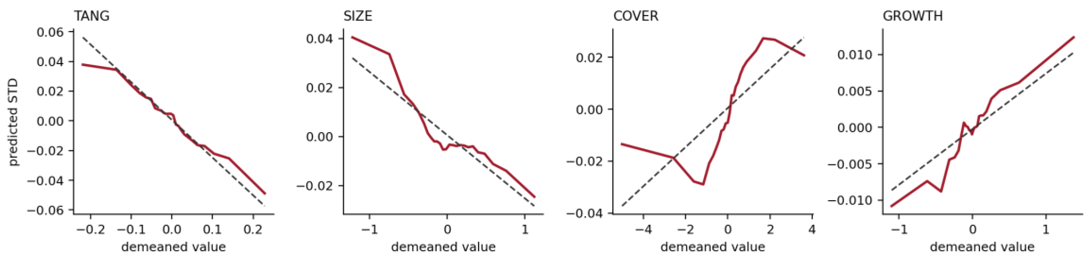
Table J1.
Local slopes of the partial-dependence curve, by tercile of the regressor.
| Variable | Linear coefficient | Tercile 1 | Tercile 2 | Tercile 3 |
|---|---|---|---|---|
| TANG | −0.2541 | −0.1763 | −0.2888 | −0.1906 |
| SIZE | −0.0258 | −0.0433 | −0.0019 | −0.0235 |
| COVER | 0.0075 | 0.0001 | 0.0292 | 0.0024 |
| GROWTH | 0.0076 | 0.0110 | 0.0030 | 0.0084 |
Note. Slopes fitted by least squares to the partial-dependence curve within each third of the grid, which spans the second to the ninety-eighth percentile of the demeaned regressor.
The pattern in the first row is the one Figure 6 shows graphically: the relationship is steepest in the middle of the distribution at −0.289 and flatter in both tails at −0.176 and −0.191, with the linear coefficient of −0.254 sitting between them and closer to the middle, which is where most of the observations are. Economically this is sensible rather than troubling. Very large within-firm swings in asset composition—a firm whose fixed-asset share moves twenty points away from its own decade average—are usually a single acquisition or disposal, and the debt structure does not follow the whole way inside the year. The other three rows show that the controls are less well described by a single slope than tangibility is, particularly interest coverage, whose effect is concentrated in the middle tercile; but since the controls are controls, this affects the fit rather than the interpretation.
Table J2.
Friedman H² between tangibility and each control.
| Pair | H² |
|---|---|
| TANG × GROWTH | 0.0299 |
| TANG × COVER | 0.0264 |
| TANG × SIZE | 0.0123 |
Note. H² is the share of the joint partial-dependence variation attributable to interaction rather than to the two separate effects, computed on a fifteen-point grid over a 4,000-observation sample. Values below 0.10 are conventionally read as no material interaction.
Figure J2.
Interaction strength and local slopes. Note. Left: H² statistics with the dashed line at the conventional 0.10 threshold. Right: local slopes of the partial-dependence curve by tercile, with the linear coefficient marked as a diamond.
Figure J2.
Interaction strength and local slopes. Note. Left: H² statistics with the dashed line at the conventional 0.10 threshold. Right: local slopes of the partial-dependence curve by tercile, with the linear coefficient marked as a diamond.
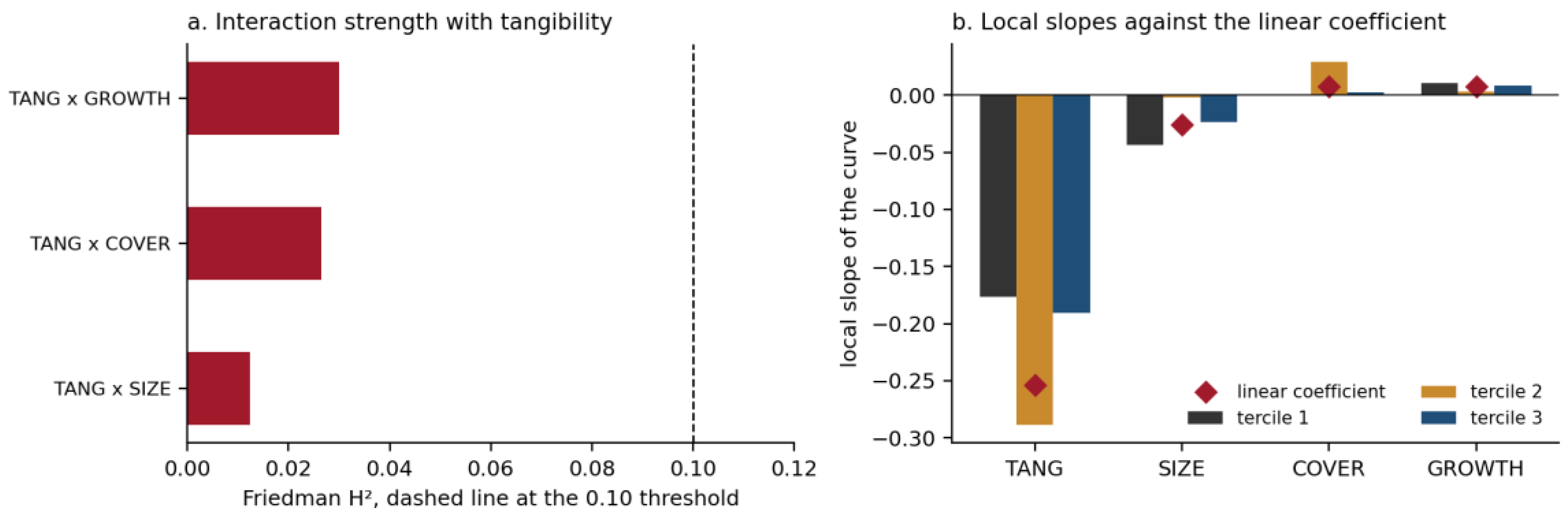
All three statistics are between a third and an eighth of the threshold, so the additive form is not concealing a moderated relationship. This has a direct consequence for the panel module: the heterogeneity documented there—flatter slopes among certified firms, flatter slopes inside the loss-making cluster—is not recoverable from an interaction with any of the four regressors in the equation. It is heterogeneity across firms, not curvature within the conditioning set, which is why it required a sample split and a taxonomy to find and could not have been picked up by adding product terms.
Appendix K. Calibration and Parametric Repair
Table K1.
Decile calibration on the held-out fold.
| Decile | Obs. | Predicted, boosting | Predicted, linear | Actual | Bias, boosting | Bias, linear |
|---|---|---|---|---|---|---|
| 1 | 1,475 | −0.0620 | −0.0482 | −0.0589 | −0.0031 | 0.0106 |
| 2 | 1,472 | −0.0279 | −0.0220 | −0.0264 | −0.0015 | 0.0044 |
| 3 | 1,473 | −0.0176 | −0.0144 | −0.0190 | 0.0013 | 0.0046 |
| 4 | 1,473 | −0.0095 | −0.0076 | −0.0144 | 0.0049 | 0.0068 |
| 5 | 1,474 | −0.0022 | −0.0026 | 0.0001 | −0.0023 | −0.0027 |
| 6 | 1,474 | 0.0047 | 0.0015 | 0.0001 | 0.0046 | 0.0014 |
| 7 | 1,472 | 0.0105 | 0.0076 | 0.0101 | 0.0004 | −0.0025 |
| 8 | 1,473 | 0.0168 | 0.0128 | 0.0180 | −0.0012 | −0.0052 |
| 9 | 1,473 | 0.0262 | 0.0227 | 0.0223 | 0.0039 | 0.0004 |
| 10 | 1,474 | 0.0627 | 0.0504 | 0.0657 | −0.0029 | −0.0152 |
Note. Observations sorted by the boosting prediction. All quantities are in units of the demeaned short-term share, so 0.0152 is 1.52 percentage points of the debt stock.
Figure K1.
Calibration and the parametric alternatives. Note. Left: mean prediction minus mean outcome by decile of predicted value. Right: out-of-sample R² of parametric expansions of the linear model, with the four-term linear specification and the boosting benchmark marked.
Figure K1.
Calibration and the parametric alternatives. Note. Left: mean prediction minus mean outcome by decile of predicted value. Right: out-of-sample R² of parametric expansions of the linear model, with the four-term linear specification and the boosting benchmark marked.
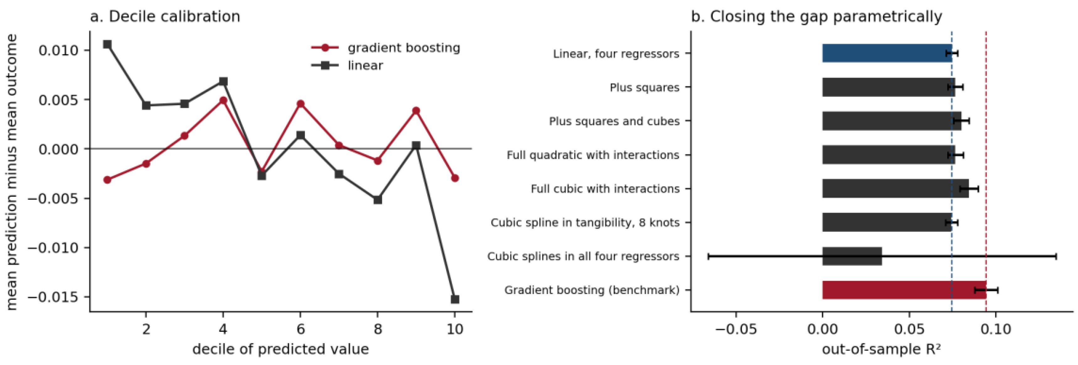
Accuracy summarised by R² conceals where a model is wrong, and the decile table locates it. Both models are unbiased in the middle of the distribution. At the ends the linear model is systematically off, under-predicting by 1.52 percentage points of the debt stock in the top decile and over-predicting by 1.06 in the bottom, while the boosting model stays inside 0.49 throughout. The pattern is monotone in the decile index, which identifies it as compression rather than misspecification: least squares shrinks the predicted range towards the mean when the underlying surface is slightly curved, and it does so symmetrically at both ends, which is exactly what Table D1 shows.
Table K2.
Can the gap be closed inside a parametric model?
| Specification | Terms | Out-of-sample R² | SD | Share of the gap closed |
|---|---|---|---|---|
| Linear, four regressors | 4 | 0.0746 | 0.0032 | — |
| Plus squares | 8 | 0.0765 | 0.0042 | 10% |
| Plus squares and cubes | 12 | 0.0802 | 0.0045 | 28% |
| Full quadratic with interactions | 14 | 0.0767 | 0.0044 | 11% |
| Full cubic with interactions | 34 | 0.0845 | 0.0051 | 50% |
| Cubic spline in tangibility, 8 knots | 13 | 0.0744 | 0.0035 | 0% |
| Cubic splines in all four regressors | 40 | 0.0342 | 0.1003 | negative |
| Gradient boosting (benchmark) | — | 0.0945 | 0.0066 | 100% |
Four readings follow. Polynomial expansion helps, but the help is modest and expensive: thirty-four terms recover half the gap, and the fold-to-fold standard deviation rises by sixty per cent as they are added, so part of what the expansion gains in fit it loses in stability. Interactions add nothing—the full quadratic with interactions scores below squares and cubes without them, which is the same message as the H² statistics reached by a different route. Splines in tangibility alone are worthless, which confirms that the mild curvature in Figure 6 is not where the residual signal is. And splines in all four regressors fail outright, with a mean R² of 0.034 and a standard deviation of 0.100 across folds, one fold having diverged entirely—the ordinary consequence of forty correlated basis functions fitted to data whose signal-to-noise ratio in the within dimension is what Table 9 says it is.
Taken together, the module supports a bounded claim and no more. Roughly a fifth of the systematic within-firm variation in debt maturity that a flexible learner can find is not available to the linear specification; the missing part is diffuse, involves no interaction with the focal regressor, does not change the sign or materially change the magnitude of the tangibility effect, and cannot be recovered by any compact parametric alternative. The linear additive form is therefore an adequate approximation for the purpose it is used for in the panel module, and the reported coefficient is not an artefact of imposing it.
Table K3.
Temporal out-of-sample validation: train on 2016–2020, test on 2021–2024.
| Linear regression | Gradient boosting | |
|---|---|---|
| Panel A. Predictive transfer | ||
| R² in the training window | 0.0640 | 0.1220 |
| R² in the forward window | 0.0771 | 0.0734 |
| RMSE in the forward window | 0.1706 | 0.1709 |
| Shrinkage from training to forward window | +0.0131 | −0.0486 |
| Panel B. Parameter transfer | β (TANG) | Boosting AME |
| Estimated on 2016–2020 | −0.2205*** (0.0166) | −0.1906 |
| Estimated on 2021–2024 | −0.2095*** (0.0160) | −0.1717 |
| Difference | −0.0109 | −0.0189 |
| Test of equality | z = −0.48, p = 0.635 | — |
Note. Dependent variable: short-term debt over total debt. Both models are fitted to firm- and year-demeaned data, with the demeaning estimated on the training window only and applied unchanged to the forward window, so that no information dated after 2020 enters the transformation. Of the 38,747 forward-window observations, 31,498 belong to a firm observed at least once in the training window and enter the forward evaluation; the remainder are firms that first file within the forward window and for which no training-window mean exists. Panel B reports two-way fixed-effects coefficients with firm-clustered standard errors in parentheses, estimated separately in each window, and the average marginal effect of tangibility from a boosting model fitted separately in each window. *** p < 0.01. The test of equality treats the two window estimates as independent.
References
- Alcock, J., Finn, F., & Tan, K.J.K. (2012). The determinants of debt maturity in Australian firms. Accounting and Finance, 52(2), 313–341. [CrossRef]
- Arcuri, M.C., & Pisani, R. (2024). Access to external credit during COVID-19: evidence from green SMEs in Italy. Review of Managerial Science, 18(7), 1–30. [CrossRef]
- Ataullah, A., Vivian, A., & Xu, B. (2018). Time-varying managerial overconfidence and corporate debt maturity structure. European Journal of Finance, 24(2), 157–181. [CrossRef]
- Bartoli, F., Ferri, G., Murro, P., & Rotondi, Z. (2013). Bank-firm relations and the role of Mutual Guarantee Institutions at the peak of the crisis. Journal of Financial Stability, 9(1), 90–104. [CrossRef]
- Belke, A. (2013). Finance access of SMEs: What role for the ECB?. Banks and Bank Systems, 8(2), 104–112.
- Bencivelli, L., & Pisicoli, B. (2022). Foreign investors and target firms’ financial structure. International Economics, 169, 230–251. [CrossRef]
- Bianchi, J., Hatchondo, J.C., & Martinez, L. (2018). International reserves and rollover risk. American Economic Review, 108(9), 2629–2670. [CrossRef]
- Boschi, M., Girardi, A., & Ventura, M. (2014). Partial credit guarantees and SMEs financing. Journal of Financial Stability, 15, 182–194. [CrossRef]
- Briozzo, A., Cardone-Riportella, C., & García-Olalla, M. (2019). Corporate governance attributes and listed SMES’ debt maturity. Corporate Governance (Bingley), 19(4), 735–750. [CrossRef]
- Butzbach, O., & Sarno, D. (2019). To what extent do regional effects influence firms’ capital structure? The case of Southern Italian SMEs’. International Journal of Financial Studies, 7(1), 3. [CrossRef]
- Byun, S.K., Lin, Z., & Wei, S. (2021). Are U.S. firms using more short-term debt?. Journal of Corporate Finance, 69, 102012. [CrossRef]
- Cai, K., Fairchild, R., & Guney, Y. (2008). Debt maturity structure of Chinese companies. Pacific Basin Finance Journal, 16(3), 268–297. [CrossRef]
- Canofari, P., Cucculelli, M., Piergallini, A., & Renghini, M. (2025). Tightening monetary policy and investment dynamics in the European Monetary Union: Firm- and country-level heterogeneity. Journal of Corporate Finance, 94, 102853. [CrossRef]
- Canto-Cuevas, F.-J., Palacín-Sánchez, M.-J., & di Pietro, F. (2016). Trade credit in SMEs: a quantile regression approach. Applied Economics Letters, 23(13), 945–948. [CrossRef]
- Cao, N., Zhang, Z., Ma, D., & Xu, D. (2026). Tax credit rating and corporate ESG performance —A dual perspective based on reputation and incentive effect. Research in International Business and Finance, 91, 103570. [CrossRef]
- Caselli, S., Corbetta, G., Cucinelli, D., & Rossolini, M. (2021). A survival analysis of public guaranteed loans: Does financial intermediary matter?. Journal of Financial Stability, 54, 100880. [CrossRef]
- Caselli, S., Corbetta, G., Rossolini, M., & Vecchi, V. (2019). Public Credit Guarantee Schemes and SMEs’ Profitability: Evidence from Italy. Journal of Small Business Management, 57(S2), 555–578. [CrossRef]
- Castaldo, A., De Luca, G., & Barile, B. (2021). Does initial access to bank loans predict start-ups’ future default probability? evidence from italy. Contemporary Economic Policy, 39(1), 83–106. [CrossRef]
- Cattafi, G., Del Pozzo, A., & Naciti, V. (2025). The Signaling Effect of Green Innovation in Accessing Bank Credit. Evidence From Italian Entrepreneurial Ventures. Business Strategy and Development, 8(4), e70247. [CrossRef]
- Cerasi, V., Fedele, A., & Miniaci, R. (2017). Product market competition and access to credit. Small Business Economics, 49(2), 295–318. [CrossRef]
- Chaturvedi, A., & Singh, A. (2024). Product market competition, debt rollover risk and financial default risk: evidence from Indian corporates. Managerial Finance, 50(10), 1837–1856. [CrossRef]
- Chen, H.J., Pan, X., Qian, M., Wu, Y., & Xia, Q. (2026). Asset pledgeability and firm innovation. Research Policy, 55(7), 105504. [CrossRef]
- Cheung, A.W.K. (2016). Corporate social responsibility and corporate cash holdings. Journal of Corporate Finance, 37, 412–430. [CrossRef]
- Chiu, W.-C., King, T.-H.D., & Wang, C.-W. (2021). Debt maturity dispersion and the cost of bank loans. Journal of Corporate Finance, 70, 102049. [CrossRef]
- Choi, J., Hackbarth, D., & Zechner, J. (2018). Corporate debt maturity profiles. Journal of Financial Economics, 130(3), 484–502. [CrossRef]
- Choi, Y.M., & Park, K. (2022). Debt maturity structure of private lodging firms. Applied Economics Letters, 29(8), 706–712. [CrossRef]
- Chu, P.K., & Kjenstad, E.C. (2023). Idiosyncratic risk and debt maturity dispersion. European Financial Management, 29(3), 930–952. [CrossRef]
- Clark, S.P., & Park, M.C. (2023). Corporate debt structure: The long and the short of it. Journal of Corporate Accounting and Finance, 34(2), 149–165. [CrossRef]
- Clemente-Almendros, J.A., Forés, B., & Camisón-Haba, S. (2024). Tourism Family Firm and Generation: Are First-Generation Firms More Conservative?. European Journal of Family Business, 14(2), 259–280. [CrossRef]
- Corredera-Catalán, F., di Pietro, F., & Trujillo-Ponce, A. (2021). Post-COVID-19 SME financing constraints and the credit guarantee scheme solution in Spain. Journal of Banking Regulation, 22(3), 250–260. [CrossRef]
- Cortez, M.A.A. (2025). Determinants of Corporate Capital Structure and the Emerging Role of Intangibles and Innovation: The Case of Japanese Corporations. DLSU Business and Economics Review, 34(2), 1–13.
- Croce, A., Quas, A., & Tenca, F. (2025). SME’s bond issuance and access to bank credit: evidence from Italy. Review of Managerial Science, 19(2), 499–535. [CrossRef]
- Cutillas Gomariz, M.F., & Sánchez Ballesta, J.P. (2014). Financial reporting quality, debt maturity and investment efficiency. Journal of Banking and Finance, 40(1), 494–506. [CrossRef]
- Dai, Y., Du, T., Gao, H., Gu, Y., & Wang, Y. (2024). Patent pledgeability, trade secrecy, and corporate patenting. Journal of Corporate Finance, 85, 102563. [CrossRef]
- D’Amato, A. (2020). Capital structure, debt maturity, and financial crisis: empirical evidence from SMEs. Small Business Economics, 55(4), 919–941. [CrossRef]
- Dang, V.A. (2011). Leverage, debt maturity and firm investment: An empirical analysis. Journal of Business Finance and Accounting, 38(1-2), 225–258. [CrossRef]
- Dang, V.A., & Phan, H.V. (2016). CEO inside debt and corporate debt maturity structure. Journal of Banking and Finance, 70, 38–54. [CrossRef]
- Dang, V.A., Gao, N., & Yu, T. (2025). Environmental Regulation and Access to Credit. British Journal of Management, 36(1), 303–322. [CrossRef]
- D’Apolito, E., Galletta, S., Iannuzzi, A.P., & Labini, S.S. (2024). Sustainability and bank credit access: New evidence from Italian SMEs. Research in International Business and Finance, 69, 102242. [CrossRef]
- Dasilas, A. (2024). Capital structure, voluntary corporate governance and credit ratings: evidence from non-listed SMEs. International Journal of Managerial and Financial Accounting, 16(1), 17–42. [CrossRef]
- Datta, S., Doan, T., & Toscano, F. (2021). Top executive gender, board gender diversity, and financing decisions: Evidence from debt structure choice. Journal of Banking and Finance, 125, 106070. [CrossRef]
- Díaz-Díaz, N.L., García-Teruel, P.J., & Martínez-Solano, P. (2016). Debt maturity structure in private firms: Does the family control matter?. Journal of Corporate Finance, 37, 393–411. [CrossRef]
- de Blasio, G., De Mitri, S., D’Ignazio, A., Finaldi Russo, P., & Stoppani, L. (2018). Public guarantees to SME borrowing. A RDD evaluation. Journal of Banking and Finance, 96, 73–86. [CrossRef]
- Della Seta, M., Morellec, E., & Zucchi, F. (2020). Short-term debt and incentives for risk-taking. Journal of Financial Economics, 137(1), 179–203. [CrossRef]
- Deng, M., & Liu, C. (2024). Sovereign risk and intangible investment. Journal of International Economics, 152, 104009. [CrossRef]
- Desogus, M., Sergi, E., & Zedda, S. (2024). The Role of Credit Consortia in the Financial Structure of Sardinian Companies During the SARS-CoV-2 Crisis. Risks, 12(12), 190. [CrossRef]
- D’Ignazio, A., & Menon, C. (2020). Causal Effect of Credit Guarantees for Small- and Medium-Sized Enterprises: Evidence from Italy. Scandinavian Journal of Economics, 122(1), 191–218. [CrossRef]
- Etudaiye-Muhtar, O.F., Ahmad, R., & Matemilola, B.T. (2017). Corporate debt maturity structure: The role of firm level and institutional determinants in selected African countries. Global Economic Review, 46(4), 422–440. [CrossRef]
- Falavigna, G., Ippoliti, R., & Ramello, G.B. (2026). Judicial uncertainty and the cost of debt: evidence from Italian SMEs. North American Journal of Economics and Finance, 85, 102670. [CrossRef]
- Fernández-Méndez, C., & González, V.M. (2019). Bank ownership, lending relationships and capital structure: Evidence from Spain. BRQ Business Research Quarterly, 22(2), 137–154. [CrossRef]
- Friewald, N., Nagler, F., & Wagner, C. (2022). Debt Refinancing and Equity Returns. Journal of Finance, 77(4), 2287–2329. [CrossRef]
- Fu, X., Huang, M., & Tang, T. (2022). Duration of executive compensation and maturity structure of corporate debt. Journal of Corporate Finance, 73, 102188. [CrossRef]
- Gai, L., Ielasi, F., & Rossolini, M. (2016). SMEs, public credit guarantees and mutual guarantee institutions. Journal of Small Business and Enterprise Development, 23(4), 1208–1228. [CrossRef]
- Gama, P.M., & Vieira, E.F. (2024). Does societal trust matter for the conservative financing policy puzzle? European SMEs evidence. Managerial Finance, 50(11), 1878–1894. [CrossRef]
- Gama, P.M., Sol Murta, F., & Vieira, E.S. (2024). Local banking development and SME conservative financing policy. Does bank branch density matter?. Small Business Economics, 63(4), 1747–1765. [CrossRef]
- Gan, G., & Valdez, E.A. (2020). Data Clustering with Actuarial Applications. North American Actuarial Journal, 24(2), 168–186. [CrossRef]
- Gao, Y., Sun, Y., & Li, Y. (2026). The effects of STAR Market reform on debt maturity mismatches of Main Board high-tech firms: Unpacking cross-board spillover effects. International Review of Economics and Finance, 111, 105663. [CrossRef]
- García-Posada, M., & Marchetti, M. (2016). The bank lending channel of unconventional monetary policy: The impact of the VLTROs on credit supply in Spain. Economic Modelling, 58, 427–441. [CrossRef]
- Gopalan, R., Mukherjee, A., & Singh, M. (2016). Do Debt Contract Enforcement Costs Affect Financing and Asset Structure?. Review of Financial Studies, 29(10), 2774–2813. [CrossRef]
- Gopalan, R., Song, F., & Yerramilli, V. (2014). Debt maturity structure and credit quality. Journal of Financial and Quantitative Analysis, 49(4), 817–842. [CrossRef]
- Greenwood, R., Hanson, S.G., & Stein, J.C. (2015). A Comparative-Advantage Approach to Government Debt Maturity. Journal of Finance, 70(4), 1683–1722. [CrossRef]
- Guglielmetti, C. (2012). Introduction: The consequences of the international crisis for European SMEs. The Consequences of the International Crisis for European SMEs: Vulnerability and Resilience, 1–16. [CrossRef]
- Haro-de-Rosario, A., Caba-Pérez, M.C., & Cazorla-Papis, L. (2016). The impact of venture capital on investee companies: evidence from Spain. Review of Managerial Science, 10(3), 577–600. [CrossRef]
- Haron, R., Nomran, N.M., Abdullah Othman, A.H., Md Husin, M., & Sharofiddin, A. (2021). The influence of firm, industry and concentrated ownership on dynamic capital structure decision in emerging market. Journal of Asia Business Studies, 15(5), 689–709. [CrossRef]
- Hassan, M.K., Karim, M.S., & Kozlowski, S.E. (2022). Implications of public corruption for local firms: Evidence from corporate debt maturity. Journal of Financial Stability, 58, 100975. [CrossRef]
- He, X.-Z., Lütkebohmert, E., & Xiao, Y. (2017). Rollover risk and credit risk under time-varying margin. Quantitative Finance, 17(3), 455–469. [CrossRef]
- Heyman, D., Deloof, M., & Ooghe, H. (2008). The financial structure of private held Belgian firms. Small Business Economics, 30(3), 301–313. [CrossRef]
- Hoffmann, A.O.I., & Kleimeier, S. (2021). Financial disclosure readability and innovative firms’ cost of debt. International Review of Finance, 21(2), 699–713. [CrossRef]
- Huberman, G., & Repullo, R. (2025). Moral hazard and debt maturity. Journal of Financial Intermediation, 61, 101121. [CrossRef]
- Hussain, H.I., Shamsudin, M.F., Salehuddin, S., & Jabarullah, N.H. (2018). Debt maturity and shari’ah compliance: Evidence from Malaysian panel data. European Research Studies Journal, 21(1), 176–186.
- Iwaki, H. (2019). The effect of debt market imperfection on capital structure and investment: Evidence from the 2008 global financial crisis in Japan. Quarterly Review of Economics and Finance, 74, 251–266. [CrossRef]
- João, I.C., Schaumburg, J., Lucas, A., & Schwaab, B. (2024). Dynamic Nonparametric Clustering of Multivariate Panel Data. Journal of Financial Econometrics, 22(2), 335–374. [CrossRef]
- Kalsie, A., & Nagpal, A. (2018). The Determinants of Corporate Debt Maturity for NSE-Listed Corporates. FIIB Business Review, 7(1), 43–56. [CrossRef]
- Kashefi Pour, E., & Khansalar, E. (2015). Does debt capacity matter in the choice of debt in reducing the underinvestment problem?. Research in International Business and Finance, 34, 251–264. [CrossRef]
- Khaw, K.L.-H., & Lee, B.C.J. (2016). Debt maturity, underinvestment problem and corporate value. Asian Academy of Management Journal of Accounting and Finance, 12, 1–17. [CrossRef]
- Körner, P. (2007). The determinants of corporate debt maturity structure: Evidence from Czech firms. Finance a Uver—Czech Journal of Economics and Finance, 57(3-4), 142–158.
- Lagazio, C., Persico, L., & Querci, F. (2021). Public guarantees to SME lending: Do broader eligibility criteria pay off?. Journal of Banking and Finance, 133, 106287. [CrossRef]
- Lee, C.-C., Wang, C.-W., Purnama, M.Y.I., & Sharma, S.S. (2024). Digitalization and firms’ debt maturity: Do financial constraints and uncertainty matter?. Pacific Basin Finance Journal, 85, 102399. [CrossRef]
- Lee, S.-T., & Jung, S.-M. (2024). Overcoming Financial Constraints on Firm Innovation: The Role of R&D Human Capital. International Journal of Financial Studies, 12(4), 109. [CrossRef]
- Li, J., Ye, Y., & Luo, R. (2026). Debt maturity structure and the quality of management earnings forecasts: evidence from China. Applied Economics Letters, 33(14), 2525–2528. [CrossRef]
- Lim, S.C., Macias, A.J., & Moeller, T. (2020). Intangible assets and capital structure. Journal of Banking and Finance, 118, 105873. [CrossRef]
- Liu, P., & Chen, S. (2023). The effect of banking deregulation on R&D investment: Evidence from the cross-regional operation of city banks. Journal of Innovation and Knowledge, 8(4), 100451. [CrossRef]
- Lopez-Gracia, J., & Mestre-Barberá, R. (2015). On the Relevance of Agency Conflicts in SME Debt Maturity Structure. Journal of Small Business Management, 53(3), 714–734. [CrossRef]
- Mabandla, N.Z., & Marozva, G. (2025). Determinants of Capital Structure: Does Growth Opportunity Matter?. Journal of Risk and Financial Management, 18(7), 385. [CrossRef]
- Magri, S. (2014). Does issuing equity help R&D activity? Evidence from unlisted Italian high-tech manufacturing firms. Economics of Innovation and New Technology, 23(8), 825–854. [CrossRef]
- Marks, J.M., & Shang, C. (2021). Does Stock Liquidity Affect Corporate Debt Maturity Structure?. Quarterly Journal of Finance, 11(1), 2150005. [CrossRef]
- McGrattan, E.R. (2020). Intangible capital and measured productivity. Review of Economic Dynamics, 37, S147–S166. [CrossRef]
- Mikrou, I., & Sapidis, N.S. (2025). A Systematic Evaluation of Clustering Algorithms Against Expert-Derived Clustering. Operations Research Forum, 6(2), 55. [CrossRef]
- Minetti, R., Murro, P., Rotondi, Z., & Zhu, S.C. (2019). Financial constraints, firms’ supply chains, and internationalization. Journal of the European Economic Association, 17(2), 327–375. [CrossRef]
- Nakatani, R. (2023). Debt maturity and firm productivity—The role of intangibles. Research in Economics, 77(1), 116–121. [CrossRef]
- Neves, M.E., Serrasqueiro, Z., Dias, A., & Hermano, C. (2020). Capital structure decisions in a period of economic intervention: Empirical evidence of Portuguese companies with panel data. International Journal of Accounting and Information Management, 28(3), 465–495. [CrossRef]
- Ng, H.C., & Cheng, F.F. (2020). The impact of financial flexibility on debt maturity structure for Australian and Malaysian firms. Afro-Asian Journal of Finance and Accounting, 10(2), 235–261. [CrossRef]
- Nguyen, C. (2022). Does amortization matter? Evidence from the syndicated loan market. Journal of Financial Research, 45(1), 92–123. [CrossRef]
- Nguyen, L., & Nguyen, C. (2020). Financial constraints, corporate debt maturity and firm performance: The case of firms in Southeast Asian countries. Afro-Asian Journal of Finance and Accounting, 10(1), 48–59. [CrossRef]
- Nouman, M., Ahmad, I., Siddiqi, M.F., Khan, F.U., Fayaz, M., & Shah, I.A. (2023). Debt maturity structure and firm investment in the financially constrained environment. International Journal of Emerging Markets, 18(10), 4613–4630. [CrossRef]
- Paeleman, I., Mataigne, V., & Vanacker, T. (2025). It Is Not All in the Debt Level: Debt Maturity Structure and Complete Export Withdrawal in International New Ventures. British Journal of Management, 36(4), 1598–1615. [CrossRef]
- Parise, G. (2018). Threat of entry and debt maturity: Evidence from airlines. Journal of Financial Economics, 127(2), 226–247. [CrossRef]
- Paseda, O., Ashade, P., Manasseh, C., & Olurin, O.E. (2026). Financial Frictions and Firm Employment Dynamics: Empirical Evidence from African Listed Firms. Journal of Applied Economic Sciences, 21(3), 951–975. [CrossRef]
- Peón, D., & Guntín, X. (2021). Bank credit and trade credit after the financial crisis: Evidence from rural galicia. Journal of Business Economics and Management, 22(3), 616–635. [CrossRef]
- Petcharat, N., & Mula, J.M. (2026). Does ESG reporting quality enhance investment efficiency? The role of debt maturity in Thailand. International Journal of Emerging Markets, 21(3), 897–920. [CrossRef]
- Phan, D.T. (2020). Factors Affecting Debt Maturity Structure: Evidence from Listed Enterprises in Vietnam. Journal of Asian Finance, Economics and Business, 7(10), 141–148. [CrossRef]
- Pinto, A.P.S., Henriques, C.M.R., Cardoso, C.E.O.D.S., & Neves, M.E.D. (2023). Bank Credit and Trade Credit: The Case of Portuguese SMEs from 2010 to 2019. Journal of Risk and Financial Management, 16(3), 170. [CrossRef]
- Pisicoli, B., Marchionne, F., & Beccari, G. (2025). Minibonds and investment: Do they promote intangible assets?. Journal of Policy Modeling, 47(6), 1222–1245. [CrossRef]
- Pongvijan, S., & Trakunphutthirak, R. (2026). An Interpretable AutoML Clustering Framework with Multi-Metric Evaluation and Generative AI-Based Explanation. 2026 9th International Conference on Artificial Intelligence and Big Data, ICAIBD 2026, 377–382. [CrossRef]
- Reale, J. (2022). Interbank market and funding liquidity risk in a stock-flow consistent model. Metroeconomica, 73(3), 734–769. [CrossRef]
- Runach, P., Garg, S., & Narwal, K.P. (2024). An Empirical Investigation on Financing Choice Descendants of Indian Start-ups. Asia-Pacific Financial Markets, 31(4), 867–888. [CrossRef]
- Shang, C. (2021). Dare to play with fire? Managerial ability and the use of short-term debt. Journal of Corporate Finance, 70, 102065. [CrossRef]
- Sinha, P., & Vodwal, S. (2023). Effect of subprime crisis on financing decisions and capital structure of Indian firms: a pre- and post- crisis study using system GMM methodology. Journal of Advances in Management Research, 20(3), 329–352. [CrossRef]
- Song, J., & Chang, F. (2025). Does judicial independence improve corporate investment efficiency?. Finance Research Letters, 85, 108248. [CrossRef]
- Tayem, G., & Altwal, F. (2023). Cash flow volatility and debt maturity structure: evidence from the gulf cooperation council countries. Journal of Governance and Regulation, 12(4), 113–123. [CrossRef]
- Tran, L.-L., Chang, C.-C., & Yu, H.-A. (2026). Considering Cluster Validity in Attribute Extension for Small Data Set Predictions. Journal of Advances in Information Technology, 17(5), 914–928. [CrossRef]
- Venugopalan, T., & Vij, M. (2014). Agency cost, growth options, and debt maturity in the indian corporate sector. Indian Journal of Finance, 8(1), 31–44.
- Vijayakumaran, S., & Vijayakumaran, R. (2019). Debt maturity and the effects of growth opportunities and liquidity risk on leverage: Evidence from Chinese listed companies. Journal of Asian Finance, Economics and Business, 6(3), 27–40. [CrossRef]
- Viswanathan, H.H.K.K., Gopinathan, K.N., & Rengasamy, S. (2026). Modelling temporal dynamics in bank ratings: a hybrid fuzzy clustering approach with the neighbourhood linkage method. Fuzzy Sets and Systems, 542, 109959. [CrossRef]
- Wang, B. (2026). Intellectual property collateralization and credit access: Evidence from patent pledging in China. Finance Research Letters, 89, 109360. [CrossRef]
- Wang, C.-W., Chiu, W.-C., & King, T.-H.D. (2020). Debt maturity and the cost of bank loans. Journal of Banking and Finance, 112, 105235. [CrossRef]
- Wang, Z., Wang, Q., & Xu, M. (2022). Short Debt Maturity and Corporate Investment: New Evidence from Chinese Listed Firms. Emerging Markets Finance and Trade, 58(9), 2453–2473. [CrossRef]
- Xiang, L. (2025). Executive-Employee Pay Gap and Corporate ESG Performance: A K-Means Analysis. Proceedings of 2025 International Conference on Economic Management and Big Data Application, ICEMBDA 2025, 326–331. [CrossRef]
- Xie, Y. (2025). Digital Inclusive Finance Drives Green Innovation: Pathways and Mechanisms for Sustainable Development. Journal of the Knowledge Economy, 16(4), 14867–14906. [CrossRef]
- Xie, Y., Wang, X., Zhang, Y., Li, B., & Yang, Y. (2026). Leveraging intellectual capital for green technology innovation: evidence from traditional manufacturing firms in China. Journal of Intellectual Capital. [CrossRef]
- Xu, N., Xu, L., & Yan, X.-W. (2025). Data factor marketization empowering enterprise innovation quality: New evidence from Chinese patent citations. International Review of Economics and Finance, 103, 104433. [CrossRef]
- Yang, T., Ma, C., Mi, X., Li, H., & Chen, D. (2026). Blockchain-embedded carbon emission allowance pledge financing: Resolving maturity mismatch with machine trust and collateral flexibility. International Journal of Production Economics, 296, 109947. [CrossRef]
- Yuan, M. (2026). Economic Policy Uncertainty and Corporate Investment Dynamics: Do Ownership and Capital Structures Matter in Listed Chinese Firms?. Pacific Economic Review, 31(2), 183–221. [CrossRef]
Figure 1.
Research design: one sample, three methods, one convergent finding. Note. The three modules share the identical 73,662 firm-year sample, so differences across them are attributable to method rather than sample construction. Each module answers a distinct question: the coefficient, its homogeneity, and the adequacy of the linear form.
Figure 1.
Research design: one sample, three methods, one convergent finding. Note. The three modules share the identical 73,662 firm-year sample, so differences across them are attributable to method rather than sample construction. Each module answers a distinct question: the coefficient, its homogeneity, and the adequacy of the linear form.
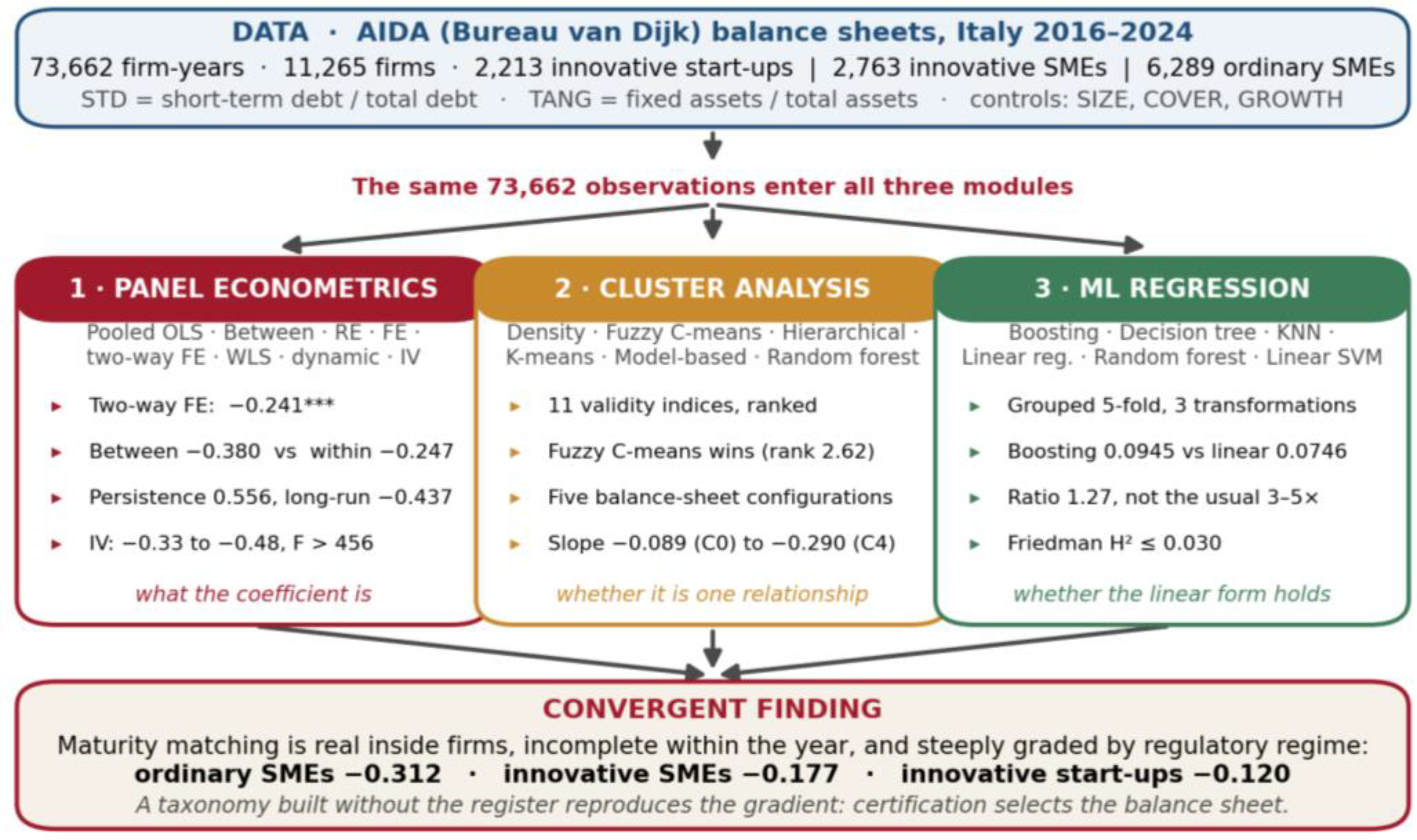
Figure 2.
The coefficient on tangibility under seven estimators, and the between–within comparison. Note. Left: point estimates with ninety-five per cent intervals; the dashed line marks the two-way fixed-effects estimate. Right: the between estimator against the within estimator, in absolute value.
Figure 2.
The coefficient on tangibility under seven estimators, and the between–within comparison. Note. Left: point estimates with ninety-five per cent intervals; the dashed line marks the two-way fixed-effects estimate. Right: the between estimator against the within estimator, in absolute value.
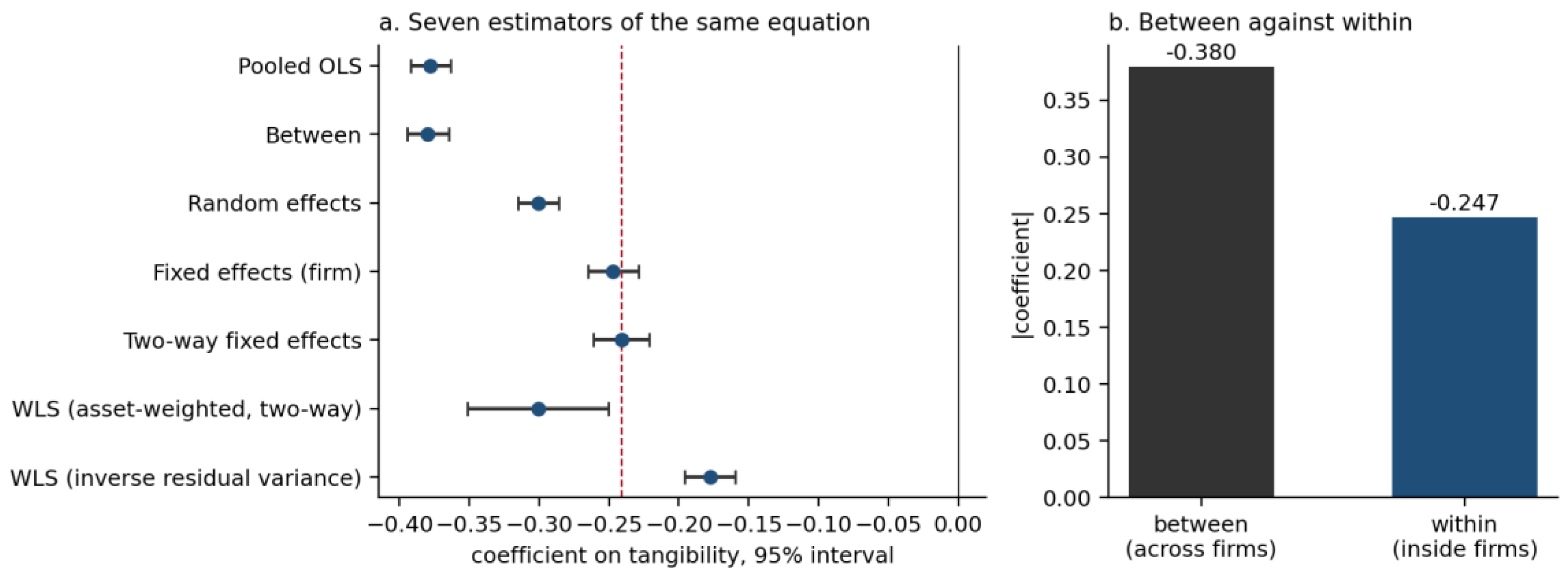
Figure 3.
The eleven indices and the aggregate ranking. Note. Left: cells report the index value; colour reports the rank of that algorithm on that index, with one the best of six. Right: mean rank across the eleven indices.
Figure 3.
The eleven indices and the aggregate ranking. Note. Left: cells report the index value; colour reports the rank of that algorithm on that index, with one the best of six. Right: mean rank across the eleven indices.
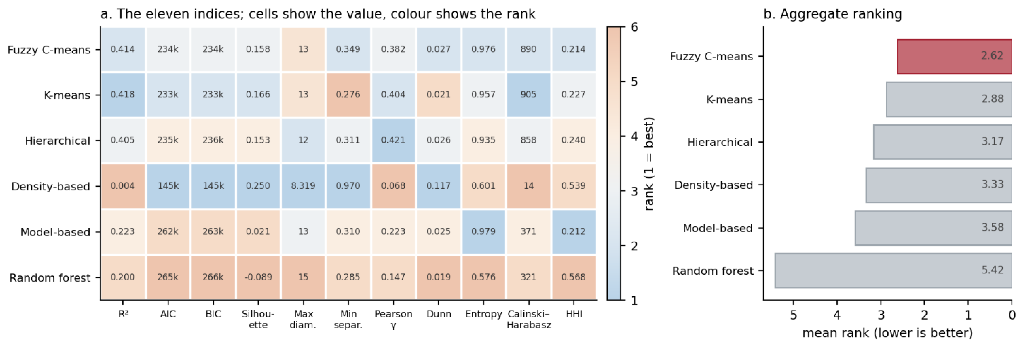
Figure 4.
The taxonomy in the plane of the two leading components. Note. Left: a random 6,000-firm subsample projected on the first two principal components. Right: the loadings that define the two axes.
Figure 4.
The taxonomy in the plane of the two leading components. Note. Left: a random 6,000-firm subsample projected on the first two principal components. Right: the loadings that define the two axes.
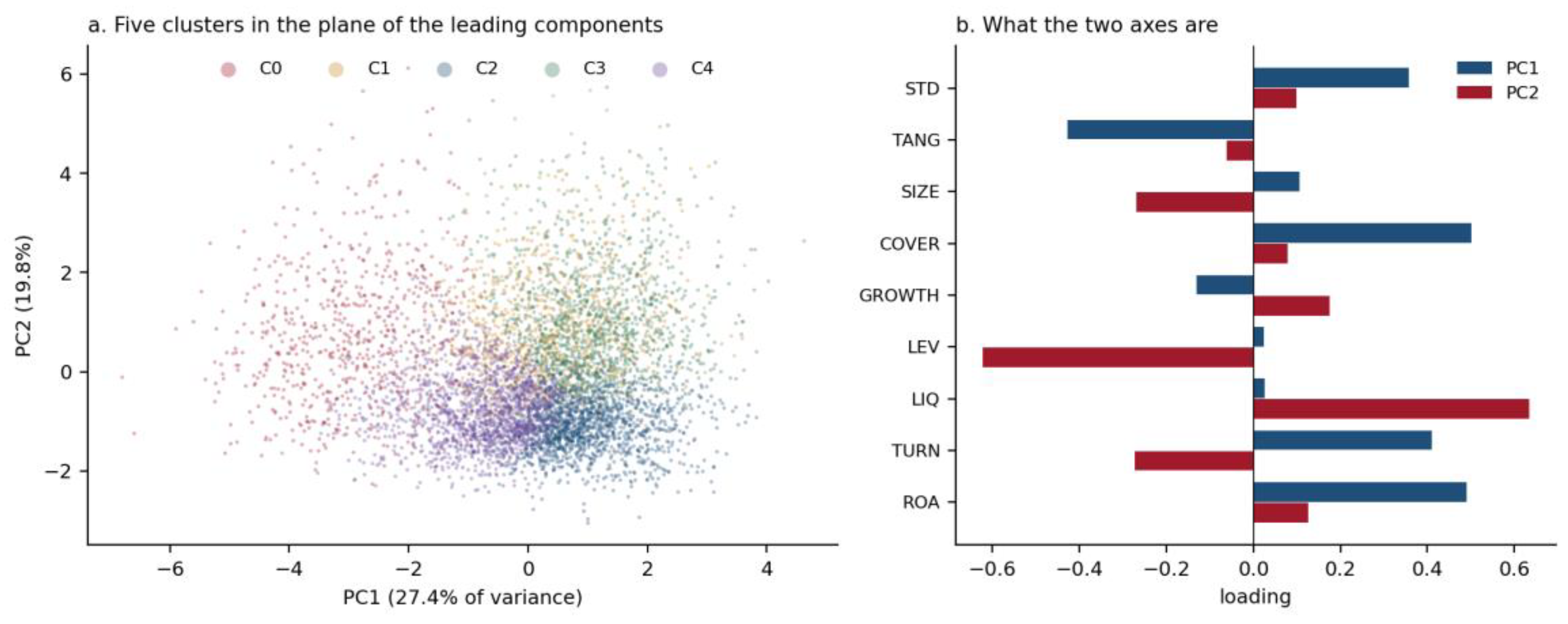
Figure 6.
What the boosting model says about the linear specification. Note. Left: loss of out-of-sample R² when each variable is permuted, ten repetitions on the held-out fold. Right: partial dependence of the predicted short-term share on tangibility, against the linear fit on the same fold.
Figure 6.
What the boosting model says about the linear specification. Note. Left: loss of out-of-sample R² when each variable is permuted, ten repetitions on the held-out fold. Right: partial dependence of the predicted short-term share on tangibility, against the linear fit on the same fold.
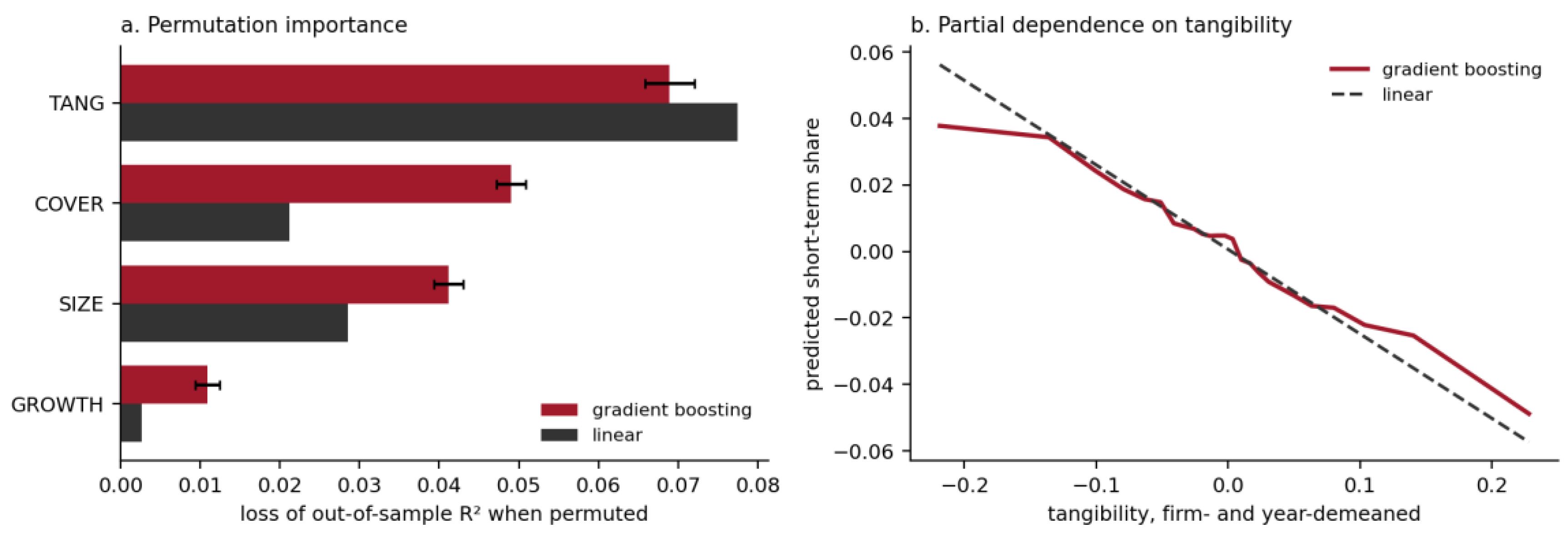
Table 1.
Where this study sits in the literature.
| Research theme | Representative studies | Main gap identified | Contribution of this study |
|---|---|---|---|
| Determinants of corporate debt maturity | Körner (2007); Cai, Fairchild & Guney (2008); Alcock, Finn & Tan (2012); Gopalan, Song & Yerramilli (2014); Choi, Hackbarth & Zechner (2018); Byun, Lin & Wei (2021); Clark & Park (2023) | Evidence is drawn almost entirely from exchange-listed firms with open access to bond markets. Tangibility enters as one control among many and is never the focal parameter, so its magnitude has been estimated hundreds of times and established once. | Makes tangibility the focal regressor on 73,662 firm-years of unlisted Italian firms, 2016–2024, with firm and year effects and firm-clustered errors. Coefficient −0.241 under two-way fixed effects, significant at one per cent under all seven estimators. |
| Debt maturity in SMEs and private firms | Heyman, Deloof & Ooghe (2008); Lopez-Gracia & Mestre-Barberá (2015); Díaz-Díaz, García-Teruel & Martínez-Solano (2016); Briozzo, Cardone-Riportella & García-Olalla (2019); D’Amato (2020); Dasilas (2024); Paeleman, Mataigne & Vanacker (2025) | Small single-country samples and short panels; identification is cross-sectional, so the comparison between firms and the comparison of a firm with itself are conflated and only the first is reported. | Reports the between estimator (−0.380) against the within estimator (−0.247) side by side. Two-thirds of the cross-sectional gradient survives firm demeaning; the residual third is composition, and is quantified rather than assumed away. |
| Tangibility, collateral and pledgeability | Gopalan, Mukherjee & Singh (2016); Lim, Macias & Moeller (2020); Dai et al. (2024); Chen et al. (2026); Wang (2026); Yang et al. (2026); Nakatani (2023) | Collateral is studied as a determinant of credit access, volume and price. The horizon of the credit obtained—the margin on which the collateral mechanism should bite hardest—is left unexamined. | Takes maturity composition as the outcome: orthogonal to the debt level by construction and to its price by observation. Both constructs are validated on two independent balance-sheet routes, correlating at 0.984 and 0.666 respectively. |
| Maturity, investment and refinancing risk | Dang (2011); Cutillas Gomariz & Sánchez Ballesta (2014); Kashefi Pour & Khansalar (2015); Della Seta, Morellec & Zucchi (2020); Friewald, Nagler & Wagner (2022); Wang, Wang & Xu (2022); Huberman & Repullo (2025) | Maturity is the regressor and investment the outcome; the determinants side is under-modelled. Static specifications impose full adjustment within the accounting year without testing it. | Bounds persistence between 0.317 and 0.721 and places the Anderson–Hsiao estimate of 0.556 inside the interval. The accumulated response to tangibility is −0.437, about 1.8 times the static coefficient. |
| Intangible-intensive and innovative firms | Magri (2014); Haro-de-Rosario, Caba-Pérez & Cazorla-Papis (2016); Hoffmann & Kleimeier (2021); Castaldo, De Luca & Barile (2021); Lee & Jung (2024); Pisicoli, Marchionne & Beccari (2025); Cattafi, Del Pozzo & Naciti (2025) | Financing-constraint research on innovative firms measures access and cost, almost never maturity composition, and rarely against a matched population of ordinary firms observed on identical items. | Estimates the same equation across three regulatory regimes drawn from one extraction: −0.120 for innovative start-ups, −0.177 for innovative SMEs, −0.312 for ordinary SMEs, with both interactions rejected at one per cent. |
| Guarantee schemes and the Italian bank–firm setting | Bartoli et al. (2013); Boschi, Girardi & Ventura (2014); Gai, Ielasi & Rossolini (2016); de Blasio et al. (2018); Caselli et al. (2019, 2021); D’Ignazio & Menon (2020); Lagazio, Persico & Querci (2021) | Guarantee evaluations measure whether credit is obtained, how much, at what price and whether the firm survives. None measures the horizon of the credit the scheme delivers. | Reads the regime gradient as the maturity margin of guaranteed short-horizon lending, and documents a monotone weakening of the cross-sectional slope from −0.400 in 2016 to −0.348 in 2024 across a decade of expanding guarantee coverage. |
| Taxonomies and model validation | João et al. (2024); Gan & Valdez (2020); Mikrou & Sapidis (2025); Tran, Chang & Yu (2026); Viswanathan, Gopinathan & Rengasamy (2026); Pongvijan & Trakunphutthirak (2026); Xiang (2025) | Applied clustering in finance typically reports one algorithm and one validity index; flexible learners enter almost exclusively as predictors and are rarely turned back on the econometric model as a specification check. | Compares six algorithms on eleven indices with rank aggregation, exposing a density-based solution that wins every geometric index by discarding 35.8 per cent of firms. Six learners are then fitted to identically demeaned data: the boosting-to-linear ratio is 1.27 and no interaction exceeds H² = 0.030. |
Note. Full references in the reference list. Coefficients quoted in the fourth column are reported in the panel, clustering and machine-learning modules respectively.
Table 2.
Variables and construction.
| Variable | Construction | AIDA source |
|---|---|---|
| STD | Short-term debt over total debt | Indice di indebitamento a breve |
| TANG | Fixed assets over total assets | (Patrimonio Netto—Margine di struttura) / Totale Attività |
| SIZE | ln total assets | Totale Attività |
| COVER | asinh(EBITDA / financial charges) | EBITDA; Totale Oneri finanziari |
| GROWTH | Δ ln revenue | Ricavi vendite e prestazioni |
Note. All continuous variables winsorised at the first and ninety-ninth percentiles within year. Standard errors clustered at firm level throughout. Sample: 2,213 innovative start-ups, 2,763 innovative SMEs and 6,289 ordinary SMEs, 2016–2024.
Table 3.
The determinants of debt maturity, six estimators.
| Pooled OLS | Between | Random eff. | Fixed effects | Two-way FE | WLS 2-way | |
|---|---|---|---|---|---|---|
| TANG | −0.3777*** (0.0074) | −0.3796*** (0.0077) | −0.3006*** (0.0073) | −0.2470*** (0.0094) | −0.2410*** (0.0102) | −0.3008*** (0.0257) |
| SIZE | −0.0073*** (0.0008) | −0.0091*** (0.0009) | −0.0202*** (0.0009) | −0.0424*** (0.0019) | −0.0437*** (0.0025) | −0.0569*** (0.0049) |
| COVER | 0.0117*** (0.0005) | 0.0118*** (0.0007) | 0.0082*** (0.0004) | 0.0070*** (0.0004) | 0.0069*** (0.0004) | 0.0091*** (0.0011) |
| GROWTH | 0.0033** (0.0016) | 0.0054 (0.0042) | 0.0057*** (0.0013) | 0.0071*** (0.0013) | 0.0103*** (0.0015) | 0.0161*** (0.0059) |
| Constant | 0.9403*** (0.0068) | 0.9585*** (0.0076) | 1.0331*** (0.0073) | 1.2097*** (0.0156) | 1.2194*** (0.0208) | 1.4373*** (0.0488) |
| Obs. | 73,662 | 11,265 | 73,662 | 73,662 | 73,662 | 73,662 |
| Firms | 11,265 | 11,265 | 11,265 | 11,265 | 11,265 | 11,265 |
| Firm effects | No | No | Random | Yes | Yes | Yes |
| Year effects | No | No | No | No | Yes | Yes |
| R² (within) | 0.063 | 0.064 | 0.084 | 0.093 | 0.092 | 0.104 |
Note. Dependent variable: short-term debt over total debt. Clustered standard errors in parentheses. *** p < 0.01, ** p < 0.05, * p < 0.10. WLS weights are total assets. The between estimator is computed on firm means, hence 11,265 observations.
Table 5.
The six algorithms.
| Family | Implementation | Settings |
|---|---|---|
| Centroid partitioning | K-means, Lloyd | k = 5, 20 restarts |
| Model-based | Gaussian mixture, full covariance | k = 5, 5 restarts |
| Fuzzy partitioning | Fuzzy C-means | c = 5, fuzzifier m = 1.5 |
| Hierarchical | Agglomerative, Ward linkage | k = 5, fitted on 5,000 firms, remainder assigned to the nearest centroid |
| Density-based | DBSCAN | ε at the median tenth-nearest-neighbour distance, min_samples = 10 |
| Random forest | Breiman synthetic contrast, 300 trees | leaf co-occurrence, 20 singular components, k = 5 |
Table 6.
The eleven indices across the six algorithms.
| Index | Fuzzy C-means | K-means | Hierarchical | Model-based | Random forest | Density-based |
|---|---|---|---|---|---|---|
| Clusters | 5 | 5 | 5 | 5 | 5 | 2 |
| Firms assigned | 100.0% | 100.0% | 100.0% | 100.0% | 100.0% | 64.2% |
| R² | 0.414 | 0.418 | 0.405 | 0.223 | 0.200 | 0.004 |
| AIC | 233,595 | 232,925 | 235,203 | 262,238 | 265,210 | 145,135 |
| BIC | 233,932 | 233,262 | 235,540 | 262,575 | 265,548 | 145,266 |
| Silhouette | 0.158 | 0.166 | 0.153 | 0.021 | −0.089 | 0.250 |
| Maximum diameter | 12.99 | 12.99 | 11.90 | 12.51 | 14.71 | 8.32 |
| Minimum separation | 0.349 | 0.276 | 0.311 | 0.310 | 0.285 | 0.970 |
| Pearson gamma | 0.382 | 0.404 | 0.421 | 0.223 | 0.147 | 0.068 |
| Dunn | 0.027 | 0.021 | 0.026 | 0.025 | 0.019 | 0.117 |
| Entropy of sizes | 0.976 | 0.957 | 0.935 | 0.979 | 0.576 | 0.601 |
| Calinski–Harabasz | 890 | 905 | 858 | 371 | 321 | 14 |
| Herfindahl–Hirschman | 0.214 | 0.227 | 0.240 | 0.212 | 0.568 | 0.539 |
| Mean rank | 2.62 | 2.88 | 3.17 | 3.58 | 5.42 | 3.33 |
Note. All indices computed on the standardised nine-dimensional firm matrix. Geometric indices use a common subsample of 5,000 firms. Noise points are excluded from the geometry and retained in the balance measures; “Assigned” is the share of firms allocated to any cluster.
Table 9.
Like-for-like comparison, linear against the best learner.
| Data transformation | Linear R² | Best learner | Its R² | Gap | Ratio |
|---|---|---|---|---|---|
| Levels (pooled) | 0.2073 (0.0158) | Gradient boosting | 0.2898 (0.0134) | 0.0825 | 1.40× |
| Levels plus firm means (Mundlak) | 0.2181 (0.0166) | Random forest | 0.2932 (0.0104) | 0.0751 | 1.34× |
| Firm- and year-demeaned (within) | 0.0746 (0.0032) | Gradient boosting | 0.0945 (0.0066) | 0.0199 | 1.27× |
Note. Fold-to-fold standard deviations in parentheses.
Table 10.
The six learners on firm- and year-demeaned data.
| Learner | Out-of-sample R² | SD | RMSE | Spearman | In-sample R² | Overfit gap |
|---|---|---|---|---|---|---|
| Gradient boosting | 0.0945 | 0.0066 | 0.1138 | 0.281 | 0.128 | 0.034 |
| Random forest | 0.0910 | 0.0068 | 0.1140 | 0.274 | 0.163 | 0.072 |
| Linear regression | 0.0746 | 0.0032 | 0.1150 | 0.246 | 0.075 | 0.001 |
| Linear SVM | 0.0728 | 0.0033 | 0.1151 | 0.249 | 0.073 | 0.000 |
| Decision tree | 0.0660 | 0.0059 | 0.1155 | 0.236 | 0.127 | 0.061 |
| K nearest neighbours | 0.0618 | 0.0059 | 0.1158 | 0.232 | 1.000 | 0.938 |
Note. Ranked by out-of-sample R². The overfitting gap is in-sample minus out-of-sample R².
Table 11.
What each method contributes relative to the existing literature.
| Method | Result obtained | Status relative to the literature |
|---|---|---|
| Pooled OLS and between estimator | Coefficient on tangibility of −0.378 and −0.380 | Confirmatory. Reproduces the magnitude reported for listed firms in an unlisted SME population. |
| Two-way fixed effects | −0.241, with the within/between decomposition reported side by side | Innovative. The within identification is standard practice elsewhere but has almost never been applied to this parameter in this population. |
| WLS, asset- and revenue-weighted | −0.301 and −0.308 | Confirmatory. The relationship is not driven by the smallest firms. |
| Dynamic panel, Anderson–Hsiao | Persistence 0.556 inside the 0.317–0.721 bound; long-run coefficient −0.437 | In opposition. Rejects the full-within-year adjustment that the static literature maintains; static estimates understate the response by about 1.8 times. |
| Instrumental variables | −0.332 to −0.480 against a first-differenced OLS of −0.211; peer instruments uninformative | In opposition. Instrumentation moves the estimate away from zero, so the received coefficient is attenuated rather than inflated by simultaneity. |
| Regime heterogeneity | −0.312 ordinary SMEs, −0.177 innovative SMEs, −0.120 innovative start-ups | Original. No prior study compares maturity determinants across certified and non-certified populations drawn from one extraction on identical items. |
| Measurement validation of both constructs | Two independent balance-sheet routes correlating at 0.984 and 0.666 | Original. The maturity literature does not ordinarily verify its dependent variable against a second construction. |
| Cluster comparison, six algorithms × eleven indices | Fuzzy C-means selected on rank aggregation; density-based wins every geometric index while discarding 35.8% of firms | In opposition. Single-index selection, still common in applied finance, would have chosen the least informative partition in the set. |
| Selected taxonomy and cluster-level slopes | Regime gradient recovered from accounts alone; Wald 56.36, p < 0.001 | Original. Supplies a test of whether the regulatory heterogeneity is an artefact of certification, which a sample split cannot provide. |
| Machine-learning regression comparison | Boosting-to-linear ratio 1.27 on demeaned data; tree and KNN below least squares | In opposition. Contradicts the multiples of three to five routinely reported, which arise from comparing learners on levels against an estimator identified within firms. |
| Interpretability diagnostics | H² ≤ 0.030; average marginal effect −0.282 against a linear −0.254; cubic expansion recovers half the gap | Confirmatory. Establishes the adequacy of the linear additive form rather than assuming it. |
Disclaimer/Publisher’s Note: The statements, opinions and data contained in all publications are solely those of the individual author(s) and contributor(s) and not of MDPI and/or the editor(s). MDPI and/or the editor(s) disclaim responsibility for any injury to people or property resulting from any ideas, methods, instructions or products referred to in the content. |
© 2026 by the authors. Licensee MDPI, Basel, Switzerland. This article is an open access article distributed under the terms and conditions of the Creative Commons Attribution (CC BY) license (http://creativecommons.org/licenses/by/4.0/).
Copyright: This open access article is published under a Creative Commons CC BY 4.0 license, which permit the free download, distribution, and reuse, provided that the author and preprint are cited in any reuse.