

Submitted:
02 September 2026
Posted:
04 September 2026
You are already at the latest version
Abstract
As microbiome research increasingly seeks to identify true ecological shifts, transitioning from associational to causal approaches is essential. However, detecting structural changes across independent networks remains challenging due to the absence of established biological ground truths and the small, imbalanced sample sizes typical of microbiome cohorts. To address this, we extend an existing network comparison framework to enable node-level mechanism-shift detection under the direct linear non-Gaussian acyclic model (DirectLiNGAM). We evaluate the Naive, Bootstrap, and Relative sample size Bootstrap Stability (RSBS) estimators across extensive synthetic discovery runs and a semi-synthetic, batch-corrected human gut microbiome cohort. Our results demonstrate that resampling-based estimation consistently outperforms a single-fit Naive baseline by trading marginal recall for substantial precision gains. On both semi-synthetic and synthetic data, standard Bootstrap is optimal for comparing datasets of equal size, whereas RSBS is the only estimator that reliably handles imbalanced cohorts. This advantage strengthens as network dimensionality increases and persists under authentic compositional noise. Navigating this complex and emerging research area is currently constrained by limitations in data quantity and quality, scarce biological knowledge, and a lack of dedicated software. To address these critical gaps, we provide the complete benchmark pipeline and synthetic data generators as an open-access Python package, causal-comparator, to support node-level mechanism-shift detection across systems biology applications.
Keywords:
causal discovery
; microbiome
; DirectLiNGAM
; mechanism shift
; network comparison
; resampling methods
; systems biology
1. Introduction
The microbiome consists of a characteristic community of microorganisms, including their genes and environmental context, that occupies a given habitat [1]. The microbiome plays a crucial role in human health. In particular, the gut microbiome has been linked to metabolic, immune, and neurological disease states [2]. A common research question in this field is to define how the abundance of specific taxa varies between distinct cohorts, such as healthy versus diseased or pre- and post-intervention [3]. The primary objective is to determine whether any detected difference reflects a genuine change in a taxon’s ecological role.
Most methods developed for this task are associational, relying on correlation-based or co-occurrence networks that are constructed separately for each group and then compared, either edge-by-edge or via global topological summaries. NetCoMi [4] formalized this workflow in a general-purpose R package, providing compositionally aware association measures, such as correlation estimators (e.g., SparCC [5]), partial correlation estimators [6], and proportionality [7], together with sparsification and formal statistical tests for whether individual edges, or the network as a whole, differ between two groups. Liu et al. [8] distilled this into a broader methodological guide for comparing co-occurrence networks constructed from different sample groups or with different construction pipelines, and Wen et al. [9] extended multi-network comparison to multi-factor, multi-treatment, and transkingdom settings. However, despite the maturity of these methods, the principle correlation is not causation remains [10]. Ultimately, the relationships identified through association-network comparisons indicate association, rather than true causal dependencies.
This reflects a growing need within the field to transition from purely associational to causal approaches [11,12]. Recent studies have begun to address this challenge directly by adapting established causal discovery algorithms to the specific characteristics of microbiome data. Sazal et al. [13] combined Bayesian networks with co-occurrence networks into a signed Bayesian network to infer directional relationships and colonization order within microbial communities, and Corander et al. [14] extended standard causal graphs to labeled DAGs that encode context-specific independence, applying the framework to identify the causal role of Clostridioides difficile in driving diarrhea risk. Transitioning from structural representation to quantitative inference, Sazal et al. [15] later used interventional calculus to estimate causal effects between taxa directly from observational abundance data. As an alternative, functional causal models leverage the statistical properties of observational data to infer directionality of relationships. Among these, DirectLiNGAM [16] is particularly well suited to taxon-level abundance data, since it guarantees identification of the causal ordering in a finite number of steps under linearity, non-Gaussian noise, and acyclicity-assumptions with reasonable justification once compositional abundances are log-ratio transformed (Section 3.6.1). MultiGroupDirectLiNGAM [17] performs a joint estimation across several datasets under the assumption that they have a common causal order, leveraging shared information across datasets to improve estimation accuracy compared to independent fitting. However, in complex biological systems, maintaining a strictly conserved causal order is rarely a realistic assumption. Consequently, imposing a shared structure can hide the exact ecological and structural shifts that a comparative analysis aims to detect. While standard DirectLiNGAM has been employed to estimate causal networks within isolated gut-microbiome cohorts [18,19,20,21], these applications do not address whether the underlying causal architecture actually changes between different groups. To bridge this gap and evaluate structural differences without forcing a shared causal ordering, one must compare independently estimated networks. Toward this end, Ma and Tourani [22] defined a resampling-based estimator for quantifying, edge by edge, how confidently an individual causal relationship differs between two learned DAGs. However, this estimator operates strictly at the edge level. It tests for isolated changes rather than assessing whether a taxon’s full regulatory mechanism (its complete set of causal parents) has shifted. In microbiome data, evaluating the entire regulatory neighborhood is often more biologically meaningful, as a taxon’s ecological role is shaped by its broader network context rather than any single interaction [23,24].
In this work, we address this gap by extending the edge-level network-comparison framework of Ma and Tourani [22] to enable node-level mechanism-shift detection under DirectLiNGAM. DirectLiNGAM is well suited to this setting because it is a computationally fast algorithm capable of operating in high-dimensional regimes and relatively small sample sizes.
The prevalence of these small datasets, coupled with frequent sample size imbalances between cohorts, motivates our choice to evaluate three distinct estimators. First, we formalize a mechanism-perturbation ground truth where an entire node’s parent set, rather than a single edge, is rewired between two systems (Section 2.2.2). We then evaluate the Naive, Bootstrap, and RSBS (Relative sample size Bootstrap Stability) estimators. The RSBS estimator is specifically designed to remain reliable when the compared datasets differ substantially in size. This addresses a critical limitation of previous associational methods, as severe sample size imbalances are the rule rather than the exception when pooling independent microbiome cohorts. We validate this framework across an extensive set of synthetic experiments spanning both equal and heterogeneous sample sizes. To ensure these findings translate to data with authentic compositional structure and non-idealized noise, we also perform a semi-synthetic validation using a batch-corrected human gut-microbiome cohort (Section 3.6). Finally, we provide the full benchmark pipeline as an open-source Python package, including the three estimators and the underlying generators for synthetic graphs and mechanism perturbations, allowing other researchers to construct their own benchmarks with known ground truths.
This study reveals that resampling-based estimation does not uniformly outperform a single-fit Naive baseline. Specifically, standard Bootstrap estimation is the superior choice when the compared datasets are of equal size. Conversely, RSBS is the only estimator that reliably outperforms the Naive approach under sample size imbalance, an advantage that becomes more pronounced as network size grows. This pattern holds in the batch-corrected gut microbiome cohort, proving that the advantages of this approach generalize beyond idealized synthetic graphs, handling real compositional and technical noise.
The remainder of this paper is organized as follows. Section 2 introduces the LiNGAM framework, DirectLiNGAM, and our proposed node-level mechanism-shift extension. Section 3 details the experimental results on fully synthetic graphs under equal and heterogeneous sample sizes, as well as the semi-synthetic microbiome validation. Finally, Section 4 and Section 5 discuss the broader implications of this work and summarize the key contributions.
2. Materials and Methods
2.1. Background: The LiNGAM Framework & DirectLiNGAM
Our approach adopts the linear, non-Gaussian acyclic model (LiNGAM) framework, originally introduced by Shimizu et al. [25], for causal discovery from purely observational data. Rather than a single algorithm, LiNGAM is a general framework that includes a variety of specific causal discovery approaches.
Among these, we focus on DirectLiNGAM [16], which relies on four core assumptions about the data-generating process: the relationships are linear, the causal structure forms a directed acyclic graph (DAG), the noise terms are non-Gaussian, and there are no unobserved confounders.
Formally, the process can be represented as a directed acyclic graph (DAG) over p variables , encoded by a adjacency matrix , where quantifies the direct causal effect of on . Let denote the position of in an unknown causal ordering, such that no variable appearing later in the ordering has a directed path to any earlier variable; under this ordering, an edge is permitted only if . Every variable is assumed to have zero mean, the data-generating process is linear, and it can be written as follows:
where are continuous random variables with non-Gaussian distributions, zero mean, and nonzero variance, and are mutually independent, so that there are no latent confounding variables. Equation (1) can be written in compact form as in Equation (2):
where is a p-dimensional random vector and is the p-dimensional error vector; can always be brought to strictly lower-triangular form by simultaneous, equal row and column permutation, as a consequence of the acyclicity assumption [26].
As an illustration, consider a three-variable causal chain , with structural equations
so that is an exogenous variable (a root node, determined only by its noise term), while and are endogenous. The corresponding adjacency matrix,
is strictly lower triangular under the causal ordering . Given observations only, the estimation problem is to recover (equivalently, the ordering together with the regression weights). Early approaches, such as ICA-LiNGAM [25], estimate the mixing matrix via independent component analysis, but suffer from the absence of guaranteed convergence to the correct solution from a poor initialization and from the need for non-trivial parameter selection. DirectLiNGAM instead estimates the causal ordering directly, by sequentially identifying exogenous variables using an independence measure. Once the ordering is estimated, is constructed by regressing each variable on its predecessors, through an adaptive LASSO.
2.1.1. DirectLiNGAM as a Causal Discovery Algorithm Reference
Throughout this paper we write M for a generic causal discovery algorithm: a procedure that takes a dataset D generated from the linear structural equation model (SEM) of Equation (2) and returns an estimated (weighted) adjacency matrix . M is treated as a black box by the Naive, Bootstrap, and RSBS estimators introduced in Section 2.2.3, which act only on (Equations (6)–(10)) and never on the internal mechanics of how M produced it. We adopt DirectLiNGAM as the concrete instantiation of M used throughout this study.
2.2. Formal Framework
2.2.1. Problem Formulation and Notation
We extend the network-comparison framework of Ma and Tourani [22], applied to the LiNGAM structural equation model of Section 2.1, from edge-level difference estimation to node-level mechanism-shift detection between a pair of systems.
Let . A system is defined by its own weighted, strictly lower-triangular matrix , generating data via the LiNGAM structural equation model of Equation (2), , i.e., . For any node k, its set of causal parents in system s is denoted by . Both systems share the same true causal order over : is always constructed from by rewiring entries within existing rows (Section 2.2.2), never by altering which index precedes which. Graphs, edge weights, and noise terms are generated following the standard DirectLiNGAM simulation protocol of Shimizu et al. [16], with the sole difference that we generate a pair of related systems, and , rather than a single one.
Baseline graphs are generated with each candidate edge , , included independently with probability (edge density). Prior to estimation, node labels are blinded independently for each system: a random permutation of is applied to the columns of , so the causal discovery algorithm M observes variables in an order unrelated to , exactly as M must recover in practice. Let denote the weighted adjacency matrix returned by M in this permuted index space. Before any comparison, each is re-aligned to the shared ground-truth order by inverting its blinding permutation, mapping row and column k back to index ; all downstream quantities are defined on these realigned matrices.
2.2.2. Mechanism-Perturbation Ground Truth
Rather than perturbing individual edges independently anywhere in the graph, as in the general formulation of in [22] (Eq. 1), our extension constrains perturbations to act on an entire node’s mechanism (its full parent set), which is the natural unit of comparison once edge-level differences are aggregated row-wise (Section 2.2.3).
Given baseline , a target set with is drawn from the subset of nodes k satisfying (enough existing parents to remove) and (enough eligible non-parent predecessors to add). For each , is obtained from by removing uniformly sampled entries from row k and adding new nonzero entries at uniformly sampled positions in row k not already in , with weights redrawn under the same protocol as Section 2.2.1. For , row k of is identical to row k of , so the structural equation for every non-target node is exactly preserved across systems. The ground truth is the binary vector
which is what the node-level estimators in Section 2.2.3 are evaluated against.
2.2.3. Estimators
For a chosen discovery algorithm M (DirectLiNGAM throughout, Section 2.1.1), let be datasets of size simulated from systems 1 and 2 via Equation (2). We extend the three estimators of [22] from the constraint-based, unweighted setting to the weighted linear-SEM setting as follows.
Naive.
A single fit of M is obtained on each dataset, and the estimated adjacency is binarized:
the direct linear-SEM analogue of Eq. 3 in [22].
2.2.3.2. Bootstrap.
M is refit on bootstrap resamples (with replacement) of each dataset, yielding the edge-selection frequency
matching Eq. 4 in [22].
RSBS (Relative sample size Bootstrap Stability).
This is our implementation’s realization of the equal-sample size resampling estimator of [22] (Eq. 5). Let . The larger of is first reduced to a single subsample of size , drawn once without replacement; the smaller dataset is left unchanged (it is already of size ). The standard bootstrap procedure of Equation (7) (with the same ) is then applied to both size- datasets:
This is a practical, single-draw simplification of the general equal-sample size resampling estimator described above, which allows for the down-sampling itself to be repeated across resamples; our implementation fixes one down-sampled subset (controlled by a random seed) and bootstraps only on top of it, trading a small amount of additional variance in the down-sampling step for a substantially lower computational cost, since only one M-fit per bootstrap replicate is required instead of two nested resampling loops.
2.2.4. From Edge-Level Differences to Node-Level Mechanism Scores
The central extension of this work is the reduction of the edge-difference matrix (for ) to a p-dimensional node score vector, aligned with the mechanism-perturbation ground truth of Equation (4). Row k of collects the estimated differences over all candidate parents of node k; summing its absolute value therefore yields a single scalar quantifying how much node k’s mechanism is estimated to have changed between the two systems:
Two properties of Equation (11) are worth making explicit. First, taking the absolute value symmetrizes the estimator: unlike the directional definition in [22] (Eq. 1), which only credits edges lost from system 1 to system 2, accumulates contributions from both edge deletions () and edge additions () at node k, matching the symmetric construction of the mechanism perturbation itself (Section 2.2.2), which always removes and adds parents. Second, because row k of contains exactly , restricting the sum to row k (rather than column k, or both) isolates changes to node k’s incoming edges, i.e., its structural mechanism, as opposed to changes in how node k influences its descendants; this is the node-level quantity that corresponds by construction to in Equation (4). The vector is evaluated against as a binary classification problem. Since is confined to the strictly lower or upper-triangular structure of , each is a nonnegative integer, or real value score with no fixed upper bound other than the row’s number of eligible entries; takes integer values (a sum of terms) and is treated as a ranking score exactly as are (a sum of -valued terms), from which AUCROC and AUPR are computed directly, and , precision, and recall are computed at the score-maximizing threshold, , searched over the set of unique observed scores (Section 3.1) as in [22].
2.3. Software Implementation
The full benchmark pipeline used to produce the synthetic results in Section 3, from graph generation through node-level scoring, is provided as an open-source Python package named causal-comparator. The complete source code is publicly available in an open repository (see the Data Availability Statement for access details).
Concretely, causal-comparator exposes the discovery algorithm M as a model_class parameter (defaulting to lingam.DirectLiNGAM), ensuring that the architecture remains modular. Beyond the three node-level estimators themselves, the software developed for this study also implements the synthetic-graph and mechanism-perturbation generators described in Section 2.2.1 and Section 2.2.2. By providing these underlying generators alongside the estimators, this framework allows researchers to construct custom benchmark datasets with known ground truths across arbitrary network sizes, edge densities, sample size regimes, and perturbation strengths.
3. Results
3.1. Experimental Design
We evaluated the Naive, Bootstrap, and RSBS estimators of Section 2 under the mechanism-perturbation ground truth of Section 2.2.2. Concretely, for a pair of systems we generated as a random strictly lower-triangular weight matrix (edge density/probability , coefficients drawn from ), and obtained by perturbing the mechanism (parent set) of a subset of target nodes: for each target, existing parents were removed and new parents were added, leaving all other nodes unchanged. Data were simulated from each system, the node labels were randomly shuffled prior to discovery to blind the causal order (as DirectLiNGAM must recover it), and the estimated adjacency/probability matrices were re-aligned to the ground-truth order before scoring. Each of the three estimators produces an edge-level difference matrix . We converted this into a node-level score, , and evaluated it against the ground-truth binary indicator of whether node k’s mechanism was perturbed, using AUCROC, AUPR, and threshold-optimized , precision, and recall. Thresholding was performed by grid search over the unique score values, as in [22]. We ran two complementary experiments. In the equal-sample size experiment, , and only the Naive and Bootstrap estimators were evaluated, since RSBS is defined only when the two sample sizes differ (Section 2.2.3). In the heterogeneous-sample size experiment, the primary and secondary dataset sizes were and respectively (yielding sample size ratios ), and all three estimators were compared. Both experiments spanned network dimensions (corresponding to p in Section 2.2.1) , edge density , (the number of target nodes with altered mechanisms), and (the number of parents swapped per target node), with 50 independently sampled seeds per configuration. For a given seed, the same pair of graphs and datasets was reused across all three estimators, allowing paired comparisons. Bootstrap and RSBS estimators utilized resamples per dataset. In total, this yielded discovery runs for the equal sample size experiment and for the heterogeneous one ( overall).
All summary tables in this section (Table 1, Table 2, Table 3, Table 4 and Table 5) aggregate over all three network sizes () unless stated otherwise. Figure 1, Figure 2 and Figure 3 and Figure 4, Figure 5 and Figure 6 show results for a representative network size of . We chose to plot a single size rather than overlaying all three, as doing so would obscure the trends in sample size and perturbation load that these figures aim to isolate. The corresponding 20 and 25 node panels are visually consistent with the trends shown and are provided as Figures S1–S6 (equal-sample size regime) and Figures S7–S12 (heterogeneous-sample size regime) in the Supplementary Materials. The size-dependent trends themselves are analyzed separately and quantitatively in Section 3.3 (Table 2), which does use all three network sizes.
3.2. Naive versus Bootstrap Estimation under Equal Sample Sizes
Table 1 summarizes performance across all runs per method in the equal-sample size experiment. Bootstrap estimation outperformed the Naive method on every ranking and classification metric except recall: mean AUPR rose from to and mean AUCROC from to . A paired comparison (same seed, same graphs, same data, differing only in estimator) confirmed this is not noise: Bootstrap exceeded Naive by AUPR (, ), AUCROC (, ), and (, ). Bootstrap’s estimates are also noticeably more stable than Naive’s. The standard deviation drops from to for AUPR, to for AUCROC, to for , and to for precision (Table 1). The one exception is recall, where Bootstrap’s SD () is marginally higher than Naive’s (). Naive only exceeded Bootstrap on recall ( vs. ; , ), at the cost of a 14-point drop in precision ( vs. ), see Section 3.5.
Figure 1 shows, for the 15-node condition, mean AUPR as a function of sample size for each edge density; the corresponding aggregate-over-all-sizes numbers are shown in Table 1– Table 2. Both methods improve monotonically with sample size, but the ordering never reverses: averaging across the three density panels shown, Bootstrap leads Naive by AUPR at ( vs. ), narrowing to a AUPR gap at ( vs. ). This same non-reversing ordering holds once the 20 and 25-node conditions are pooled in, at lower absolute AUPR (Table 1), because larger networks are harder to discover from a fixed, small sample (Table 2). Edge density has only a minor effect on the gap; both curves shift slightly as the graph becomes sparser, consistent with fewer high-effect-size parents to anchor discovery.
Figure 2 stress-tests the estimators (15-node condition) as the fraction of perturbed nodes increases (holding ). Bootstrap’s advantage over Naive is stable across densities and perturbation fractions, indicating the benefit of resampling is not an artifact of a specific graph topology or perturbation load; the same qualitative pattern, at correspondingly lower absolute AUPR, holds in the 20 and 25-node conditions (Table 2).
Figure 3 examines the effect of perturbation strength (parents swapped per target node) on precision and recall, again for the 15-node condition at the highest edge density tested (). Increasing from 1 to 2 raises precision for both methods (Naive: ; Bootstrap: ), consistent with a larger effect size making the perturbation easier to detect, while recall remains high () for both methods.
3.3. Effect of Network Size
Table 2 reports AUCROC and AUPR as the number of nodes grows from 15 to 25, with the (small) sample sizes used in our grid held fixed. Performance degrades for every method as dimensionality increases, as expected given the growing number of parameters DirectLiNGAM must estimate; but the size of the drop is not uniform across estimators. For Naive, AUPR falls from (15 nodes) to (25 nodes), a 30-point drop; for Bootstrap, it falls from to , a smaller relative decline that leaves Bootstrap’s advantage over Naive larger at 25 nodes ( AUPR) than at 15 ( AUPR). The same pattern holds in the heterogeneous experiment (Section 3.4), where RSBS’s margin over Naive widens from AUPR at 15 nodes to at 25 nodes. Resampling-based confidence therefore becomes more valuable as the discovery problem gets harder.
3.4. Naive versus Bootstrap versus RSBS under Heterogeneous Sample Sizes
When the two datasets differ substantially in size, the ranking among estimators changes in an important way: plain Bootstrap resampling is no longer reliably better than the Naive method. Over all runs of the heterogeneous experiment (Table 3), Bootstrap’s mean AUCROC () and () were lower than Naive’s ( and ), and the paired difference was significant (AUCROC: , , ; : , , ), though the AUPR difference was not distinguishable from zero (, , ). RSBS, designed specifically for this regime, was the only estimator that dominated Naive on every metric except recall (AUPR , ; AUCROC , ; , ; all ) and also outperformed plain Bootstrap on every metric except recall (AUPR , AUCROC , ; all ). Under the same evaluation framework, RSBS achieved or shared the top performance in of the 198 heterogeneous parameter combinations, versus for Bootstrap and for Naive.
Figure 4 shows, for the 15-node condition, mean AUPR against the larger sample size , marginalized over . RSBS (top curve) leads throughout; Naive (bottom curve at low density, middle at higher density) and Bootstrap cross over depending on density, reflecting the non-uniform Bootstrap-vs-Naive result above.
Figure 5 repeats the topological stress test of Figure 2 in the heterogeneous regime. RSBS sits above both Naive and Bootstrap at every density and every perturbation load tested, consistent with the overall ranking in Table 3.
Figure 6 shows precision and recall vs. perturbation strength for the 15-node condition at the highest edge density tested (). As in the equal-sample size experiment, increasing from 1 to 2 raises precision for all three methods (Naive: ; Bootstrap: ; RSBS: ), and RSBS’s precision advantage over Bootstrap is concentrated at (the harder, single-parent-swap condition), where RSBS also has the edge over Naive.
Table 4 breaks the heterogeneous experiment down by sample size ratio . RSBS’s advantage is largest exactly where it is designed to help: at the most imbalanced ratio (, i.e., , ), RSBS beats Naive by AUPR and Bootstrap by AUPR (paired and , both ; see Table 5), while plain Bootstrap is statistically indistinguishable from Naive on AUPR at this ratio (, , ) despite being worse on AUCROC (, , ). As (equal sample sizes), the three methods converge, and RSBS becomes numerically indistinguishable from Bootstrap (AUCROC vs. ; AUPR vs. at )—exactly as expected, since the equal-sample size resampling step in Equation 10 performs no downsampling when and RSBS reduces to standard bootstrap by construction. This internal consistency check gives us additional confidence in the correctness of our LiNGAM adaptation of the CausalComparator estimators.
3.5. The Precision–Recall Trade-off across Both Regimes
A consistent pattern emerges across both experiments: the Naive method achieves the highest recall of the three estimators but the lowest precision, in essentially every configuration we tested (Table 1 and Table 3). Because Naive assigns a hard edge label from a single DirectLiNGAM fit per dataset, it has no mechanism to discount edges that are only weakly or inconsistently supported by the data; borderline edges are as likely to flip the node-level score as strongly supported ones. This over-flags a wider set of nodes as perturbed, inflating recall while depressing precision. In the equal-sample size experiment, Naive’s recall () exceeds Bootstrap’s () by only 2 points, while its precision () trails Bootstrap’s () by 14 points. In the heterogeneous experiment, Naive’s recall () exceeds RSBS’s () by 4 points, while its precision () trails RSBS’s () by 7 points; the gap widens further under the most imbalanced sample sizes tested (: Naive precision vs. RSBS , a 9-point gap against a 8-point recall deficit). In every configuration we examined, the precision gain for the resampling-based estimators exceeded their recall cost, which is why they dominate on , AUPR, and AUCROC despite never leading on recall alone. This trade-off is most pronounced exactly where discovery is hardest—at the smallest sample sizes and under the greatest sample size imbalance (Table 4, )—suggesting that the confidence information carried by resampling is most useful precisely when a single point-estimate discovery run is least trustworthy.
3.6. Semi-Synthetic Benchmark Derived from Human Gut Microbiome Data
3.6.1. Cohort Construction
To assess whether the findings of Section 3.2, Section 3.3, Section 3.4 and Section 3.5 transfer beyond fully synthetic graphs, we applied the same three estimators to a real gut-microbiome cohort drawn from curatedMetagenomicData (version 3.16.1) [27], a curated, uniformly reprocessed collection of publicly available human microbiome shotgun-sequencing studies. We restricted to disease-free adult stool samples (, , ), excluded samples with recorded current antibiotic use, pregnancy, or lactation, applied a minimum sequencing-depth floor of reads [28,29], and retained one sample per subject (earliest visit, in studies with repeated sampling), to avoid pseudo-replication from longitudinally resampled individuals. This yielded samples spanning multiple independent studies. Species-level relative abundances were aggregated to the family level; families present in fewer than of samples or averaging less than relative abundance were dropped [30,31], leaving 24 families.
Because samples originate from different studies, we corrected for study-level technical batch effects with MMUPHin [32] (adjust_batch, batch variable = study, applied on the relative-abundance scale prior to log-ratio transformation), then applied a centered log-ratio (CLR) transform [33,34] to remove the compositional (sum-to-one) constraint inherent to relative-abundance data, which otherwise induces spurious negative correlations among taxa unrelated to any real biological association. A quick diagnostic check (a one-way, Euclidean-distance analogue of PERMANOVA on the CLR-transformed family profile) confirmed that study identity explained of total compositional variance prior to correction, supporting a non-negligible batch effect worth correcting for. Because the full 24-family CLR composition sums to exactly zero for every sample by construction, its coordinates are linearly dependent, so the resulting covariance structure has rank at most for p parts rather than full rank [33], a well-known obstacle in compositional data analysis that also affects CLR-based microbial network inference specifically [6]. Any full-rank parameterization of a p-part composition must be -dimensional; standard constructions include the isometric log-ratio basis and Aitchison’s additive log-ratio, which fixes one part as reference and is equivalent, up to a linear transformation, to dropping one CLR coordinate [33,35]. We adopted the latter in its simplest form, dropping the single highest-mean-CLR family (Lachnospiraceae) prior to modeling, leaving 23 usable, well-posed variables.
3.6.2. Semi-Synthetic Ground Truth Construction
A fundamental obstacle in validating causal discovery or causal inference methods on gut microbiome data, and on microbiome data more generally, is the near-total absence of biological ground truth. Communities with fully known interaction sets are rare, and existing validated interaction lists are incomplete rather than exhaustive. No such resource exists at the scale this cohort operates at (thousands of samples, dozens of taxa). As a result, evaluation of microbial network inference is still carried out largely in silico, using synthetic or semi-synthetic data rather than communities with fully known interactions [36]. Fully synthetic graphs (Section 2.2.1) let us control the ground truth exactly, but say nothing about whether the estimators remain informative once applied to data with real compositional structure and real non-idealized noise. We therefore constructed a semi-synthetic ground truth. It inherits this cohort’s actual compositional structure and residual noise, but includes a known, injected structural change against which detection performance can still be measured directly. For each node count , treated independently, we selected the p most abundant families from the pool of 23 usable families described in Section 3.6.1 and fit a separate real DirectLiNGAM model (Section 2.1.1) to the full -sample cohort restricted to just those p families. Fitting the baseline on the full cohort, and only subsequently drawing smaller simulated samples from it for evaluation, follows the same real-data design used by Ma and Tourani [22] in their own real-world evaluation, where causal graphs were likewise estimated on the full sample size of each real dataset before subsampling for the comparison experiment. This produces three independent baseline fits, one per node count, each with its own causal order , adjacency matrix , and residuals implied by that fit.
We ranked families by mean CLR value, rather than sampling them at random, for two reasons. First, low-abundance taxa are disproportionately affected by zero-inflation and detection-limit noise, which degrades the reliability of any network or causal structure built on them [36]; restricting to the families with the highest mean CLR value at each p favors the more reliably measured taxa, consistent with the prevalence/abundance filter already applied during cohort construction (Section 3.6.1). Second, ranking by mean CLR value produces nested panels across node counts (15-family ⊂ 20-family ⊂ 23-family), so that increasing p consistently means adding progressively rarer, harder-to-estimate families.
was then perturbed into using exactly the mechanism-perturbation procedure of Section 2.2.2 (Equation (4)): target nodes have parent edges removed and new parent edges added, with new-edge weights built by drawing a magnitude from the empirical distribution of ’s nonzero weights and assigning an independent random sign, so injected edges have plausible magnitudes and can be positive or negative, just like the real network’s own edges. What differs from the fully synthetic setup of Section 2.2.1 is where the baseline graph, causal order, and noise come from, and how data are subsequently simulated: instead of a randomly generated graph and fresh i.i.d. noise from a specified non-Gaussian distribution, the baseline and are estimated directly from the real cohort, and each of the two simulated datasets is generated as , where is built by bootstrap-resampling rows of the real residual matrix . Resampling whole residual rows, rather than resampling each family’s residual independently, preserves whatever real cross-family residual dependence the linear fit did not absorb; using the empirical residual distribution as-is, rather than fitting a parametric noise model to it, avoids introducing a further, potentially misspecified, distributional assumption on top of the real data.
Therefore, it is worthwhile to mention that is itself a DirectLiNGAM fit, not independently verified ground truth about the true causal structure of the human gut microbiome. Moreover, this design does not test whether DirectLiNGAM recovers the true biological network. It tests whether the Naive, Bootstrap, and RSBS estimators can reliably detect a controlled, known structural change injected on top of a real, data-derived baseline, under real noise, real edge scale, and a real causal order, rather than a synthetic one.
3.6.3. Experimental Design
For every combination, twenty independent replicates were run, each drawing a new random target set T, simulating samples from and from (sample size ratio , held fixed rather than swept, unlike the synthetic heterogeneous experiment of Section 3.4), and scoring all three estimators with 100 bootstrap resamples each. We tested (the last using the full 23-family panel), (equivalently – of nodes perturbed, depending on p), and parent edges swapped per perturbed node. This gives 18 parameter combinations repeats runs per estimator, discovery-comparison runs in total. Metrics (AUCROC, AUPR, threshold-optimized , precision, recall) are computed exactly as in Section 2.2.4.
3.6.4. Results
Table 6 reports overall performance, split by perturbation intensity . Pooled across all 18 conditions (360 paired runs), both resampling-based estimators outperformed Naive by a statistically significant margin: Bootstrap led Naive by AUCROC (, ), AUPR (, ), and (, ); RSBS led Naive by AUCROC (, ), AUPR (, ), and (, ). Bootstrap and RSBS, in contrast, were not distinguishable from each other pooled over all conditions (AUCROC , ; AUPR , ), at the single, moderate sample size ratio () used throughout this cohort. This is a narrower separation between the two resampling-based estimators than in the synthetic heterogeneous experiment at the same ratio (Section 3.4, Table 4, where RSBS still led Bootstrap by AUPR at ), consistent with the additional biological and technical noise present in real, compositional microbiome data relative to a clean synthetic linear SEM.
Figure 7 shows mean AUPR against node count p, faceted by . Absolute performance is markedly lower than on the fully synthetic graphs of Section 3.2, Section 3.3 and Section 3.4 (AUPR in the – range here, versus – there), which is expected: real, batch-corrected, compositional microbiome data carries genuine biological and technical noise that a clean synthetic linear SEM does not, and should not be expected to match. More informative than the absolute level is the trend across p: Bootstrap’s advantage over the other two estimators, clearest at (AUCROC vs. RSBS vs. Naive ), erodes as p grows, and by the ranking has reversed on both ranking metrics — RSBS leads (AUCROC , AUPR ), with Bootstrap (/) statistically indistinguishable from Naive (/) on AUCROC. This mirrors, within the microbiome-derived semi-synthetic benchmark, the qualitative pattern already established synthetically in Section 3.3: resampling-based confidence becomes more valuable, not less, as the discovery problem gets harder, and here RSBS specifically is the estimator that keeps that promise as network size grows.
Figure 8 repeats the topological stress test of Figure 2 and Figure 5 on the real cohort, faceted by p instead of edge density (the real cohort’s structural axis). The same crossover is visible panel-by-panel: at , Bootstrap leads at every perturbation load tested; by , RSBS leads at every perturbation load tested, with the gap most pronounced at the lowest perturbation fraction shown ().
Table 7 reports the paired comparison at the hardest condition tested (largest node count, strongest perturbation: , ). RSBS’s advantage over Naive is significant on AUPR (, , ) and (, , ) even at this reduced, condition-specific sample size ( paired repeats); its advantage over Bootstrap on AUPR is directionally consistent but only borderline significant at this single condition (, , ), while Bootstrap is statistically indistinguishable from Naive on every metric at this hardest condition, consistent with the crossover already visible in Figure 7.
Finally, Figure 9 examines the effect of perturbation strength itself on precision and recall, pooled over all three node counts. Increasing from 2 to 4 raised precision for every method (Naive: ; Bootstrap: ; RSBS: ), while recall stayed essentially flat for all three (– throughout). This is the same qualitative pattern as Figure 3 and Figure 6: a larger injected structural change is easier to distinguish from background noise without any corresponding cost in the estimators’ sensitivity, and its replication here, on a real, batch-corrected, compositional cohort rather than a synthetic graph, is itself a validity check on the estimators’ behavior: despite the added difficulty of real, compositional, batch-corrected data, effect size still behaves the way it should.
3.7. Summary of Findings
- Under equal sample sizes, Bootstrap dominated the Naive estimator on AUCROC, AUPR, , and precision across every network size, edge density, and perturbation setting tested (best-or-tied in of 99 parameter combinations, vs. for Naive).
- Under heterogeneous sample sizes, plain Bootstrap resampling lost its advantage over the Naive method (and was significantly worse on AUCROC and ), confirming that resampling alone does not compensate for unequal discovery power between datasets of very different sizes.
- RSBS (equal-sample size resampling) was the most robust estimator overall in the heterogeneous experiment, best-or-tied in of 198 parameter combinations, with its largest advantage precisely at the most imbalanced sample size ratio tested ().
- RSBS converges to plain Bootstrap as the sample size ratio approaches 1, as it must by construction, which we take as an internal validity check on our LiNGAM implementation of the three estimators.
- Performance for all three estimators degraded as the number of nodes grew from 15 to 25 at fixed (small) sample sizes, but the relative benefit of resampling-based estimation over the Naive method increased with network size, rather than diminishing.
- Across both experiments, the Naive method consistently achieved the highest recall but the lowest precision; Bootstrap and RSBS traded a small amount of recall for a substantially larger gain in precision, which drove their advantage on , AUPR, and AUCROC.
- Because gut microbiome data lack an established causal ground truth and are compositional, with CLR-transformed abundances rank-deficient by construction, evaluating the estimators on real data required a purpose-built, semi-synthetic, real-data-grounded validation (Section 3.6.2) rather than a direct comparison against known structure.
- On this real, batch-corrected microbiome cohort, both resampling-based estimators reproduced the synthetic experiments’ qualitative ranking, outperforming Naive by a modest but statistically significant margin (pooled across node counts and perturbation intensities), though Bootstrap and RSBS were not distinguishable from each other at the single, moderate sample size ratio tested, a narrower separation than observed in the synthetic heterogeneous experiment at the same ratio.
4. Discussion
As the need for mechanistic approaches to discover ecological shifts in microbial communities grows, transitioning from purely associational to causal methods has become essential. Traditional comparative methods rely on correlational summaries. However, these approaches cannot reliably distinguish true mechanistic changes from purely associational differences. To address this limitation, we extended the network comparison framework of Ma and Tourani [22] to detect mechanism shifts at the node level under DirectLiNGAM. We evaluated three estimators, Naive, Bootstrap, and RSBS, that are designed to handle the small and often imbalanced sample sizes typical of microbiome data.
Our empirical evaluation across fully synthetic networks and a semi-synthetic gut microbiome cohort reveals that the optimal estimation strategy depends fundamentally on the sample size. When comparing datasets of equal size, standard Bootstrap estimation consistently dominated the Naive baseline across all tested network sizes, edge densities, and perturbation settings. However, this advantage deteriorated under heterogeneous sample sizes because plain Bootstrap failed to compensate for unequal discovery power. In these imbalanced scenarios, the RSBS estimator was the only method that reliably outperformed the Naive approach. We specifically designed RSBS to equalize sample sizes prior to resampling. As the network size increased and the discovery problem became more difficult, the relative benefit of estimation based on resampling grew. The underlying mechanism for this performance gain is rooted in a trade-off between precision and recall. While the Naive method achieves high recall, it suffers from poor precision by overestimating weakly supported edges. Both Bootstrap and RSBS trade a marginal reduction in recall for a substantial increase in precision. This property proved robust even when subjected to the authentic compositional and technical noise of a real microbiome cohort corrected for batch effects.
Despite these promising results, we must acknowledge several limitations. First, an absolute and independently verified causal network for the human gut microbiome does not currently exist. Therefore, our real-world validation relied on a semi-synthetic ground truth. While our findings confirm that the estimators can detect structural shifts against a baseline derived from data, they do not guarantee that DirectLiNGAM perfectly recovers the true underlying biological network. Second, the framework operates under the assumption of no unobserved confounders. In microbial ecosystems, unmeasured variables like host metabolites or environmental factors can act as hidden common causes that drive the apparent relationship between two species [15]. Third, DirectLiNGAM relies on linearity and acyclicity. In contrast, true microbial interactions frequently feature complex nonlinear dynamics and feedback loops that violate the directed acyclic graph (DAG) assumption [37]. Finally, our current synthetic validation was computationally constrained to a moderate number of nodes. Capturing microbiome dynamics at the species level naturally involves significantly higher dimensionality.
Future work will focus on addressing these dimensional limitations by extending the synthetic benchmarking to accommodate more than 50 variables. This expansion is a necessary prerequisite before applying the pipeline at the species level. It will require expanded computational resources and optimized hardware configurations. Ultimately, we aim to extend the framework along with the Python package to evaluate different classes of structural perturbations in other fields. For example, we could model gene knockout experiments in broader systems biology applications.
5. Conclusions
In this study, we extended the network comparison framework of Ma and Tourani [22] to detect node-level mechanism shifts under DirectLiNGAM. We rigorously evaluated three estimators (Naive, Bootstrap, and RSBS) across nearly 40,000 synthetic discovery runs and a semi-synthetic, batch-corrected human gut microbiome cohort. Our findings demonstrate that estimation based on resampling consistently outperforms a single-fit Naive baseline. Specifically, standard Bootstrap is optimal for equal sample sizes, while RSBS is the only estimator that reliably handles imbalanced cohorts.
The complete benchmark pipeline, named causal-comparator, is openly available as a Python package hosted in a public GitHub repository. We designed this framework specifically to accommodate custom structural perturbations and dynamic synthetic data generation. As a result, researchers can easily adapt and extend the pipeline to generate their own benchmarks with known ground truths. Because of its flexible architecture, causal-comparator is not restricted to the microbiome field, but serves as a general-purpose tool for causal mechanism-shift detection across broader systems biology applications.
Supplementary Materials
Figure S1: Learning curves, equal sample sizes, 20-node condition; Figure S2: Topological stress test, equal sample sizes, 20-node condition; Figure S3: Intervention complexity, equal sample sizes, 20-node condition; Figure S4: Learning curves, equal sample sizes, 25-node condition; Figure S5: Topological stress test, equal sample sizes, 25-node condition; Figure S6: Intervention complexity, equal sample sizes, 25-node condition; Figure S7: Learning curves, heterogeneous sample sizes, 20-node condition; Figure S8: Topological stress test, heterogeneous sample sizes, 20-node condition; Figure S9: Intervention complexity, heterogeneous sample sizes, 20-node condition; Figure S10: Learning curves, heterogeneous sample sizes, 25-node condition; Figure S11: Topological stress test, heterogeneous sample sizes, 25-node condition; Figure S12: Intervention complexity, heterogeneous sample sizes, 25-node condition.
Author Contributions
FC: Conceptualization, Data curation, Formal Analysis, Investigation, Methodology, Project administration, Resources, Software, Validation, Visualization, Writing – original draft, Writing – review and editing. EA: Conceptualization, Funding acquisition, Investigation, Resources, Supervision, Validation, Visualization, Writing – original draft, Writing – review and editing. FS: Conceptualization, Data curation, Formal Analysis, Funding acquisition, Investigation, Methodology, Project administration, Resources, Software, Supervision, Validation, Visualization, Writing – original draft, Writing – review and editing. All authors have read and agreed to the published version of the manuscript.
Funding
This research was funded by Minutia.AI Pte. Ltd.
Institutional Review Board Statement
Not applicable.
Informed Consent Statement
Not applicable.
Data Availability Statement
The software developed for this study, including the Naive, Bootstrap, and RSBS node-level estimators and the synthetic-graph and mechanism-perturbation generation framework, is openly available as the causal-comparator package on GitHub at https://github.com/Francesco-Canonaco/causal-comparator, allowing the full benchmark pipeline to be reproduced. The underlying real microbiome data are publicly available via curatedMetagenomicData [27].
Acknowledgments
The authors thank Nicole Astrologo for her help in retrieving the curated metagenomic data. During the preparation of this manuscript/study, the author(s) used GenAI for the purposes of code review and text review. The authors have reviewed and edited the output and take full responsibility for the content of this publication. All computational experiments were performed on an Amazon Web Services Elastic Compute Cloud (AWS EC2) c6a.8xlarge instance running Ubuntu Server 24.04 LTS (64-bit x86). The instance was equipped with 32 vCPUs (16 physical AMD EPYC 7R13 cores with two threads per core) and 64 GiB of RAM.
Conflicts of Interest
Author FC is funded by Minutia.AI Pte. Ltd. Author EA has equity and is an advisor to Minutia.AI Pte. Ltd. The remaining author(s) declared that this work was conducted in the absence of any commercial or financial relationships that could be construed as a potential conflict of interest.
Abbreviations
The following abbreviations are used in this manuscript:
| AUCROC | Area Under the Receiver Operating Characteristic Curve |
| AUPR | Area Under the Precision–Recall Curve |
| CI | Confidence Interval |
| CLR | Centered Log-Ratio |
| DAG | Directed Acyclic Graph |
| ICA | Independent Component Analysis |
| LASSO | Least Absolute Shrinkage and Selection Operator |
| PERMANOVA | Permutational Multivariate Analysis of Variance |
| RSBS | Relative sample size Bootstrap Stability |
| SD | Standard Deviation |
| SEM | Structural Equation Model |
References
- Berg, G.; Rybakova, D.; Fischer, D.; Cernava, T.; Vergès, M.C.C.; Charles, T.; Chen, X.; Cocolin, L.; Eversole, K.; Corral, G.H.; et al. Microbiome definition re-visited: old concepts and new challenges. Microbiome 2020, 8, 103. [Google Scholar] [CrossRef] [PubMed]
- Hou, K.; Wu, Z.X.; Chen, X.Y.; Wang, J.Q.; Zhang, D.; Xiao, C.; Zhu, D.; Koya, J.B.; Wei, L.; Li, J.; et al. Microbiota in health and diseases. Signal Transduct. Target. Ther. 2022, 7, 135. [Google Scholar] [CrossRef] [PubMed]
- Wang, Y.; Zhou, J.; Ye, J.; Sun, Z.; He, Y.; Zhao, Y.; Ren, S.; Zhang, G.; Liu, M.; Zheng, P.; et al. Multi-omics reveal microbial determinants impacting the treatment outcome of antidepressants in major depressive disorder. Microbiome 2023, 11, 195. [Google Scholar] [CrossRef] [PubMed]
- Peschel, S.; Müller, C.L.; Von Mutius, E.; Boulesteix, A.L.; Depner, M. NetCoMi: network construction and comparison for microbiome data in R. Brief. Bioinform. 2021, 22, bbaa290. [Google Scholar] [CrossRef] [PubMed]
- Friedman, J.; Alm, E.J. Inferring correlation networks from genomic survey data. 2012. [Google Scholar] [CrossRef] [PubMed]
- Kurtz, Z.D.; Müller, C.L.; Miraldi, E.R.; Littman, D.R.; Blaser, M.J.; Bonneau, R.A. Sparse and compositionally robust inference of microbial ecological networks. PLoS Comput. Biol. 2015, 11, e1004226. [Google Scholar] [CrossRef] [PubMed]
- Lovell, D.; Pawlowsky-Glahn, V.; Egozcue, J.J.; Marguerat, S.; Bähler, J. Proportionality: a valid alternative to correlation for relative data. PLoS Comput. Biol. 2015, 11, e1004075. [Google Scholar] [CrossRef] [PubMed]
- Liu, C.; Li, C.; Jiang, Y.; Zeng, R.J.; Yao, M.; Li, X. A guide for comparing microbial co-occurrence networks. Imeta 2023, 2, e71. [Google Scholar] [CrossRef] [PubMed]
- Wen, T.; Liu, Y.X.; Liu, L.; Niu, G.; Ding, Z.; Teng, X.; Ma, J.; Liu, Y.; Yang, S.; Xie, P.; et al. ggClusterNet 2: An R package for microbial co-occurrence networks and associated indicator correlation patterns. Imeta 2025, 4, e70041. [Google Scholar] [CrossRef] [PubMed]
- Pearl, J. Causality; Cambridge university press, 2009. [Google Scholar]
- Moreno-Indias, I.; Lahti, L.; Nedyalkova, M.; Elbere, I.; Roshchupkin, G.; Adilovic, M.; Aydemir, O.; Bakir-Gungor, B.; Santa Pau, E.C.d.; D’Elia, D.; et al. Statistical and Machine Learning Techniques in Human Microbiome Studies: Contemporary Challenges and Solutions. Front. Microbiol. 2021, 12–2021. [Google Scholar] [CrossRef] [PubMed]
- Khelfaoui, I.; Wang, W.; Meskher, H.; Shehata, A.I.; El Basuini, M.F.; Abouelenein, M.F.; Degha, H.E.; Alhoshy, M.; Teiba, I.I.; Mahmoud, S.S. Beyond just correlation: Causal machine learning for the microbiome, from prediction to health policy with econometric tools. Front. Microbiol. 2025, 16, 1691503. [Google Scholar] [CrossRef] [PubMed]
- Sazal, M.; Mathee, K.; Ruiz-Perez, D.; Cickovski, T.; Narasimhan, G. Inferring directional relationships in microbial communities using signed Bayesian networks. BMC Genom. 2020, 21, 663. [Google Scholar] [CrossRef] [PubMed]
- Corander, J.; Hanage, W.P.; Pensar, J. Causal discovery for the microbiome. Lancet Microbe 2022, 3, e881–e887. [Google Scholar] [CrossRef] [PubMed]
- Sazal, M.; Stebliankin, V.; Mathee, K.; Yoo, C.; Narasimhan, G. Causal effects in microbiomes using interventional calculus. Sci. Rep. 2021, 11, 5724. [Google Scholar] [CrossRef] [PubMed]
- Shimizu, S.; Inazumi, T.; Sogawa, Y.; Hyvarinen, A.; Kawahara, Y.; Washio, T.; Hoyer, P.O.; Bollen, K.; Hoyer, P. DirectLiNGAM: A direct method for learning a linear non-Gaussian structural equation model. J. Mach. Learn. Res.-JMLR 2011, 12, 1225–1248. [Google Scholar]
- Shimizu, S. Joint estimation of linear non-Gaussian acyclic models. Neurocomputing 2012, 81, 104–107. [Google Scholar] [CrossRef]
- Miyajima, Y.; Karashima, S.; Ogai, K.; Taniguchi, K.; Ogura, K.; Kawakami, M.; Nambo, H.; Kometani, M.; Aono, D.; Demura, M.; et al. Impact of gut microbiome on dyslipidemia in japanese adults: Assessment of the Shika-machi super preventive health examination results for causal inference. Front. Cell. Infect. Microbiol. 2022, 12, 908997. [Google Scholar] [CrossRef] [PubMed]
- Koshida, A.; Karashima, S.; Ogura, K.; Miyajima, Y.; Ogai, K.; Mizoguchi, R.; Ikagawa, Y.; Hara, S.; Mizushima, I.; Fujii, H.; et al. Impact of gut microbiome on serum IgG4 levels in the general population: Shika-machi super preventive health examination results. Front. Cell. Infect. Microbiol. 2023, 13, 1272398. [Google Scholar] [CrossRef] [PubMed]
- Miyajima, Y.; Karashima, S.; Mizoguchi, R.; Kawakami, M.; Ogura, K.; Ogai, K.; Koshida, A.; Ikagawa, Y.; Ami, Y.; Zhu, Q.; et al. Prediction and causal inference of hyperuricemia using gut microbiota. Sci. Rep. 2024, 14, 9901. [Google Scholar] [CrossRef] [PubMed]
- Canonaco, F.; Acerbi, E.; Stella, F. Improving DirectLiNGAM for high-dimensional microbiome data: roots screening and eBIC based model selection. Front. Syst. Biol. 2026, 6, 1835323. [Google Scholar] [CrossRef] [PubMed]
- Ma, S.; Tourani, R. Comparing Causal Bayesian Networks Estimated from Data. Entropy 2024, 26, 228. [Google Scholar] [CrossRef] [PubMed]
- Lv, B.M.; Quan, Y.; Zhang, H.Y. Causal inference in microbiome medicine: principles and applications. Trends Microbiol. 2021, 29, 736–746. [Google Scholar] [CrossRef] [PubMed]
- Luo, M.; Zhu, J.; Jia, J.; Zhang, H.; Zhao, J. Progress on network modeling and analysis of gut microecology: a review. Appl. Environ. Microbiol. 2024, 90, e00092–24. [Google Scholar] [CrossRef] [PubMed]
- Shimizu, S.; Hoyer, P.O.; Hyvärinen, A.; Kerminen, A.; Jordan, M. A linear non-Gaussian acyclic model for causal discovery. J. Mach. Learn. Res. 2006, 7. [Google Scholar]
- Bollen, K.A. Structural equations with latent variables; John Wiley & Sons, 1989. [Google Scholar]
- Pasolli, E.; Schiffer, L.; Manghi, P.; Renson, A.; Obenchain, V.; Truong, D.T.; Beghini, F.; Malik, F.; Ramos, M.; Dowd, J.B.; et al. Accessible, curated metagenomic data through ExperimentHub. Nat. Methods 2017, 14, 1023–1024. [Google Scholar] [CrossRef] [PubMed]
- Hillmann, B.; Al-Ghalith, G.A.; Shields-Cutler, R.R.; Zhu, Q.; Gohl, D.M.; Beckman, K.B.; Knight, R.; Knights, D. Evaluating the information content of shallow shotgun metagenomics. Msystems 2018, 3, 10–1128. [Google Scholar] [CrossRef] [PubMed]
- Treichel, N.S.; Pauvert, C.; Séneca, J.; Pjevac, P.; Berry, D.; Penders, J.; Hitch, T.C.; Clavel, T. Benchmarking of shotgun sequencing depth reveals the potential and limitations of shallow metagenomics and strain-level analysis. Nat. Microbiol. 2026, 1–12. [Google Scholar] [CrossRef] [PubMed]
- Neu, A.T.; Allen, E.E.; Roy, K. Defining and quantifying the core microbiome: challenges and prospects. Proc. Natl. Acad. Sci. 2021, 118, e2104429118. [Google Scholar] [CrossRef] [PubMed]
- Bokulich, N.A.; Subramanian, S.; Faith, J.J.; Gevers, D.; Gordon, J.I.; Knight, R.; Mills, D.A.; Caporaso, J.G. Quality-filtering vastly improves diversity estimates from Illumina amplicon sequencing. Nat. Methods 2013, 10, 57–59. [Google Scholar] [CrossRef] [PubMed]
- Ma, S.; Shungin, D.; Mallick, H.; Schirmer, M.; Nguyen, L.H.; Kolde, R.; Franzosa, E.; Vlamakis, H.; Xavier, R.; Huttenhower, C. Population structure discovery in meta-analyzed microbial communities and inflammatory bowel disease using MMUPHin. Genome Biol. 2022, 23, 208. [Google Scholar] [CrossRef] [PubMed]
- Aitchison, J. The statistical analysis of compositional data. J. R. Stat. Soc. Ser. B (Methodological) 1982, 44, 139–160. [Google Scholar] [CrossRef]
- Gloor, G.B.; Macklaim, J.M.; Pawlowsky-Glahn, V.; Egozcue, J.J. Microbiome datasets are compositional: and this is not optional. Front. Microbiol. 2017, 8, 2224. [Google Scholar] [CrossRef] [PubMed]
- Hron, K.; Filzmoser, P.; Thompson, K. Linear regression with compositional explanatory variables. J. Appl. Stat. 2012, 39, 1115–1128. [Google Scholar] [CrossRef]
- Faust, K. Open challenges for microbial network construction and analysis. ISME J. 2021, 15, 3111–3118. [Google Scholar] [CrossRef] [PubMed]
- Coyte, K.Z.; Schluter, J.; Foster, K.R. The ecology of the microbiome: networks, competition, and stability. Science 2015, 350, 663–666. [Google Scholar] [CrossRef] [PubMed]
Figure 1.
Mean AUPR (with 95% CI band) for detecting perturbed-mechanism nodes as a function of sample size, for the Naive and Bootstrap estimators under equal sample sizes (), faceted by edge density. Shown for the 15-node network-size condition (see Table 2 for the 20 and 25-node aggregate numbers, and Figures S1 and S4 in the Supplementary Materials for the corresponding 20- and 25-node charts).
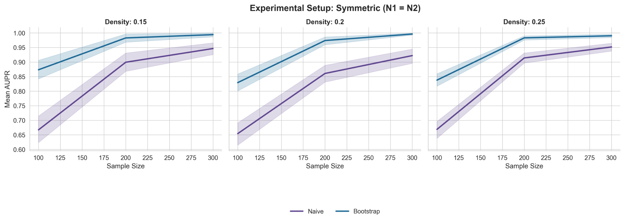
Figure 2.
Mean AUPR as the percentage of perturbed nodes increases, by edge density, for Naive and Bootstrap under equal sample sizes. 15-node network-size condition.
Figure 2.
Mean AUPR as the percentage of perturbed nodes increases, by edge density, for Naive and Bootstrap under equal sample sizes. 15-node network-size condition.
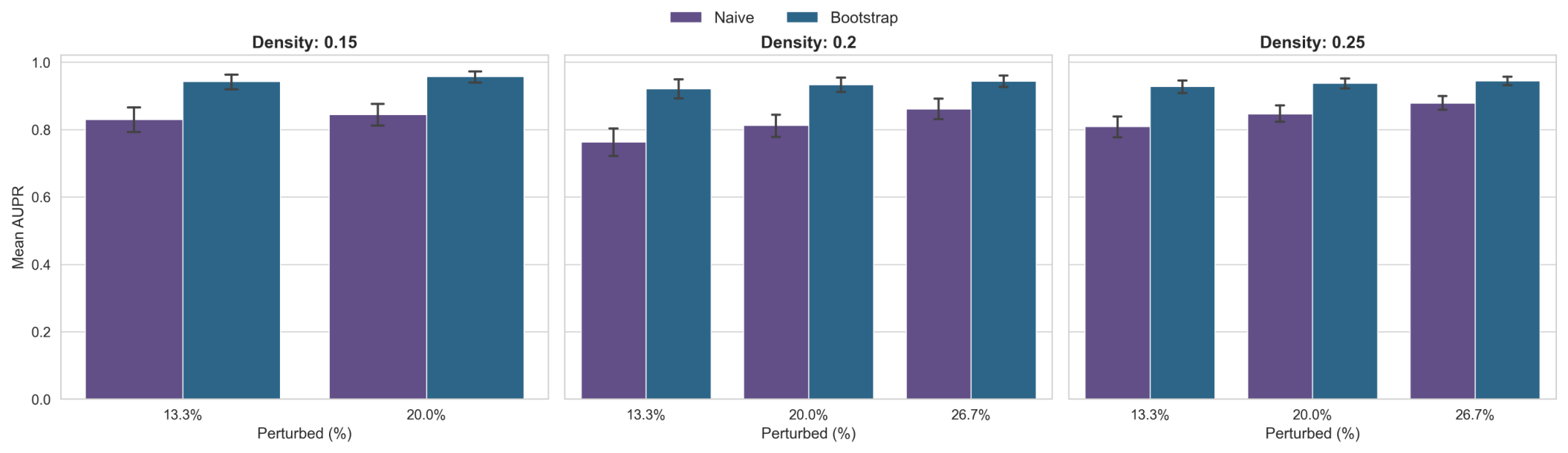
Figure 3.
Precision and recall as a function of the number of parents swapped per perturbed node (), for Naive and Bootstrap, at the highest edge density tested (). 15-node network-size condition.
Figure 3.
Precision and recall as a function of the number of parents swapped per perturbed node (), for Naive and Bootstrap, at the highest edge density tested (). 15-node network-size condition.
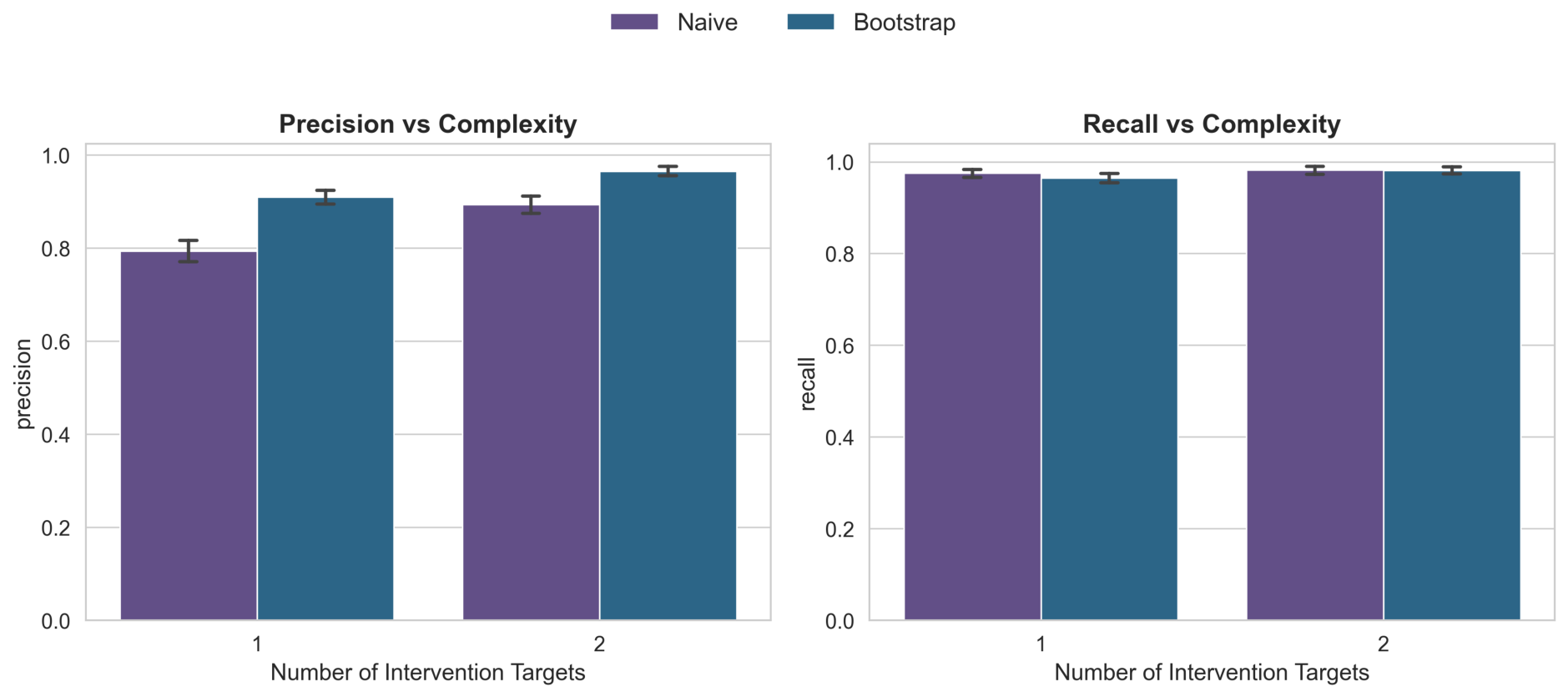
Figure 4.
Mean AUPR (95% CI band) against the primary sample size , marginalized over , for Naive, Bootstrap, and RSBS under heterogeneous sample sizes, faceted by edge density. 15-node network-size condition (see Table 2 for the 20 and 25-node aggregate numbers, and Figures S7 and S10 in the Supplementary Materials for the corresponding 20- and 25-node charts).
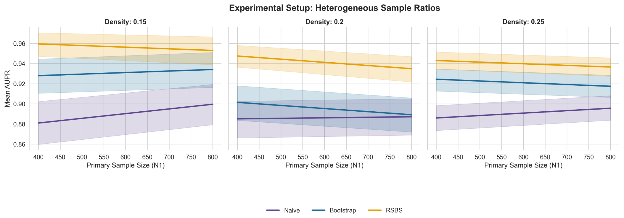
Figure 5.
Mean AUPR as the percentage of perturbed nodes increases, by edge density, for Naive, Bootstrap, and RSBS under heterogeneous sample sizes. 15-node network-size condition.
Figure 5.
Mean AUPR as the percentage of perturbed nodes increases, by edge density, for Naive, Bootstrap, and RSBS under heterogeneous sample sizes. 15-node network-size condition.
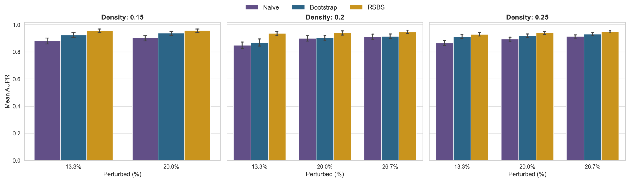
Figure 6.
Precision and recall as a function of the number of parents swapped per perturbed node (), for Naive, Bootstrap, and RSBS under heterogeneous sample sizes, at the highest edge density tested (). 15-node network-size condition.
Figure 6.
Precision and recall as a function of the number of parents swapped per perturbed node (), for Naive, Bootstrap, and RSBS under heterogeneous sample sizes, at the highest edge density tested (). 15-node network-size condition.
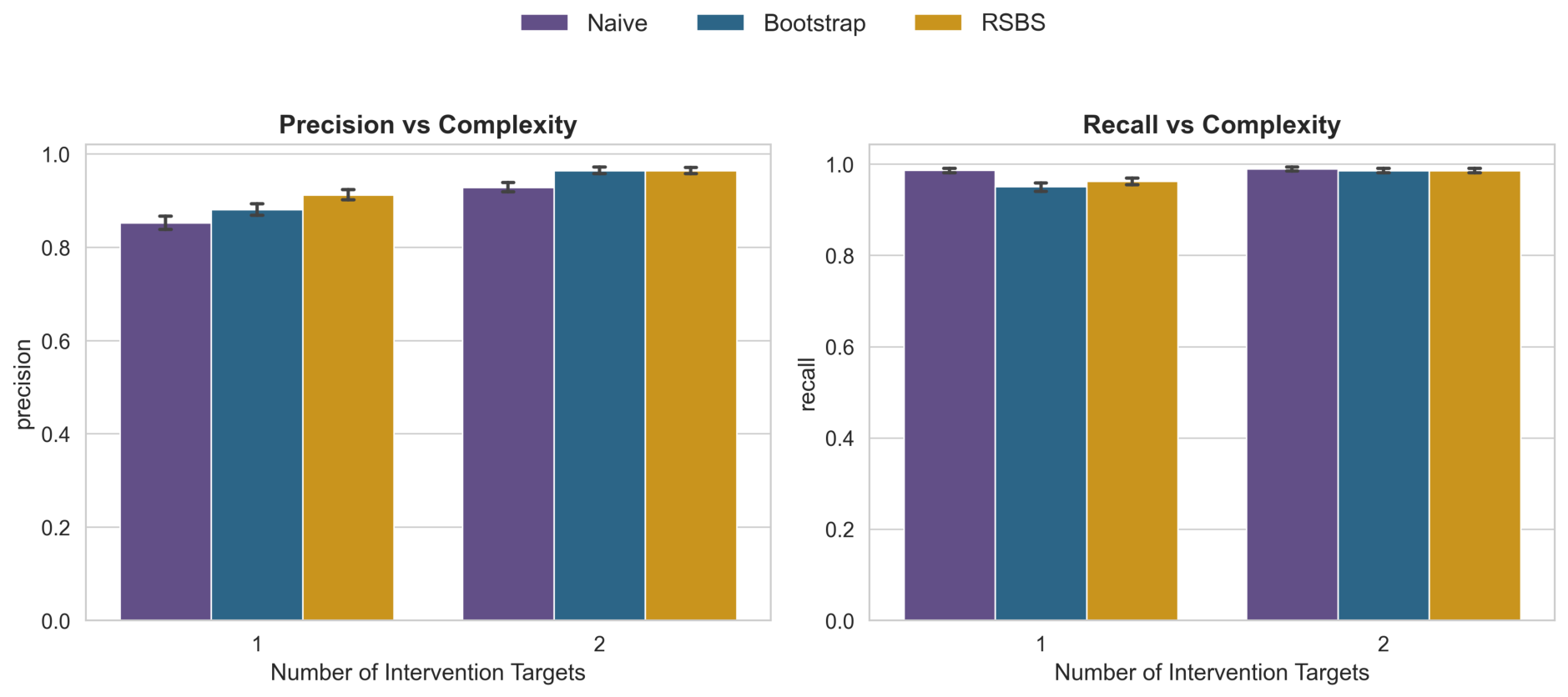
Figure 7.
Mean AUPR (with 95% CI band) against node count p for the real microbiome cohort, faceted by perturbation intensity .
Figure 7.
Mean AUPR (with 95% CI band) against node count p for the real microbiome cohort, faceted by perturbation intensity .
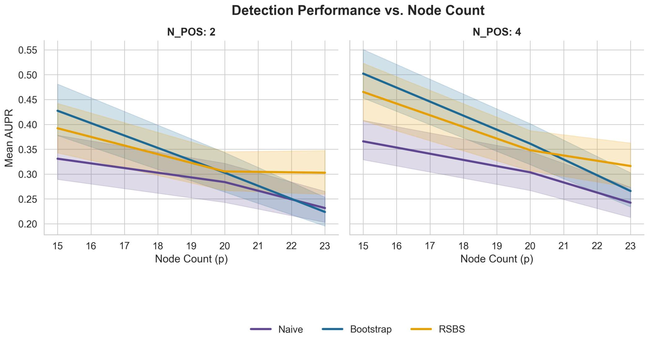
Figure 8.
Mean AUPR as the percentage of perturbed nodes increases, faceted by node count p, for Naive, Bootstrap, and RSBS on the real microbiome cohort.
Figure 8.
Mean AUPR as the percentage of perturbed nodes increases, faceted by node count p, for Naive, Bootstrap, and RSBS on the real microbiome cohort.
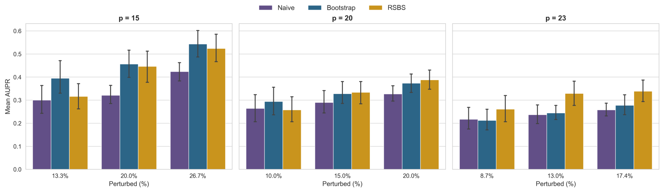
Figure 9.
Precision and recall as a function of the number of parents swapped per perturbed node (), for Naive, Bootstrap, and RSBS on the real microbiome cohort, pooled over .
Figure 9.
Precision and recall as a function of the number of parents swapped per perturbed node (), for Naive, Bootstrap, and RSBS on the real microbiome cohort, pooled over .
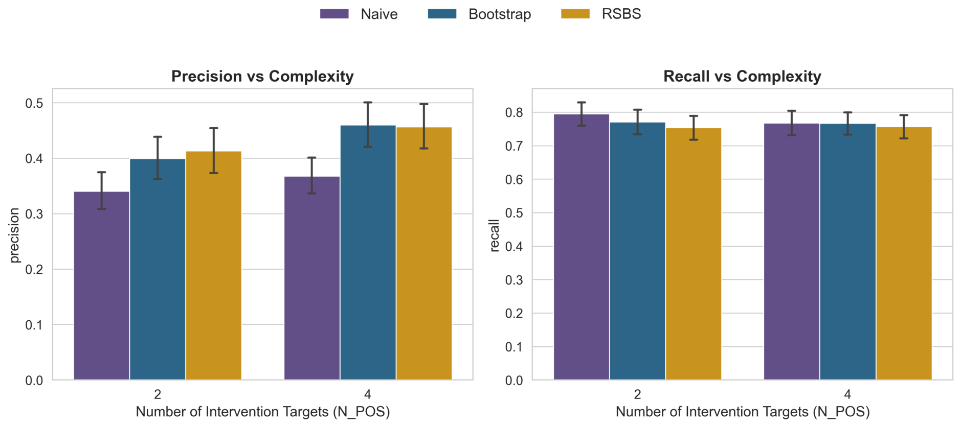

Table 1.
Overall performance under equal sample sizes (), mean ± SD over runs per method.
| Method | AUCROC | AUPR | Precision | Recall | |
|---|---|---|---|---|---|
| Naive | 0.894 ± 0.142 | 0.687 ± 0.296 | 0.760 ± 0.233 | 0.699 ± 0.291 | 0.945±0.153 |
| Bootstrap | 0.941 ± 0.103 | 0.825 ± 0.244 | 0.853 ± 0.193 | 0.837 ± 0.237 | 0.926 ± 0.164 |
Table 2.
Effect of network size on mean AUCROC / AUPR (SD omitted for brevity).
| Experiment | Method | 15 nodes | 20 nodes | 25 nodes |
|---|---|---|---|---|
| Equal () | Naive | 0.946 / 0.834 | 0.895 / 0.687 | 0.839 / 0.538 |
| Bootstrap | 0.976 / 0.938 | 0.941 / 0.831 | 0.903 / 0.706 | |
| Heterogeneous | Naive | 0.965 / 0.889 | 0.931 / 0.764 | 0.885 / 0.636 |
| Bootstrap | 0.965 / 0.916 | 0.911 / 0.764 | 0.843 / 0.602 | |
| RSBS | 0.978 / 0.943 | 0.943 / 0.838 | 0.900 / 0.707 |
Note: Bold values indicate the best performance for each metric.
Table 3.
Overall performance under heterogeneous sample sizes (), mean ± SD over runs per method.
| Method | AUCROC | AUPR | Precision | Recall | |
|---|---|---|---|---|---|
| Naive | 0.927 ± 0.117 | 0.764 ± 0.278 | 0.824 ± 0.214 | 0.772 ± 0.272 | 0.966 ± 0.122 |
| Bootstrap | 0.907 ± 0.133 | 0.761 ± 0.288 | 0.802 ± 0.230 | 0.786 ± 0.280 | 0.904 ± 0.188 |
| RSBS | 0.941 ± 0.105 | 0.829 ± 0.246 | 0.857 ± 0.196 | 0.844 ± 0.238 | 0.927 ± 0.165 |
Note: Bold values indicate the best performance for each metric.
Table 4.
Mean AUCROC / AUPR by sample size ratio in the heterogeneous experiment.
| Method | ||||
|---|---|---|---|---|
| Naive | 0.837 / 0.553 | 0.900 / 0.694 | 0.973 / 0.869 | 0.981 / 0.902 |
| Bootstrap | 0.808 / 0.550 | 0.862 / 0.654 | 0.958 / 0.868 | 0.995 / 0.972 |
| RSBS | 0.858 / 0.629 | 0.913 / 0.758 | 0.983 / 0.930 | 0.995 / 0.972 |
Note: Bold values indicate the best performance for each metric.
Table 5.
Paired comparison at the most imbalanced ratio evaluated (, , paired runs). Mean difference (row method − column method), paired t-statistic and p-value.
Table 5.
Paired comparison at the most imbalanced ratio evaluated (, , paired runs). Mean difference (row method − column method), paired t-statistic and p-value.
| Comparison | AUCROC | AUPR | |
|---|---|---|---|
| RSBS − Naive | (, ) | (, ) | (, ) |
| RSBS − Bootstrap | (, ) | (, ) | (, ) |
| Bootstrap − Naive | (, ) | (, , n.s.) | (, ) |
Table 6.
Overall performance in the microbiome-derived semi-synthetic benchmark, mean ± SD over 180 runs per method per row, split by perturbation intensity (parent edges swapped per perturbed node), pooled over and .
Table 6.
Overall performance in the microbiome-derived semi-synthetic benchmark, mean ± SD over 180 runs per method per row, split by perturbation intensity (parent edges swapped per perturbed node), pooled over and .
| Method | AUCROC | AUPR | Precision | Recall | ||
|---|---|---|---|---|---|---|
| 2 | Naive | 0.552 ± 0.181 | 0.282 ± 0.160 | 0.405 ± 0.136 | 0.341 ± 0.235 | 0.795 ± 0.242 |
| Bootstrap | 0.572 ± 0.179 | 0.318 ± 0.192 | 0.437 ± 0.151 | 0.399 ± 0.275 | 0.771 ± 0.255 | |
| RSBS | 0.583 ± 0.181 | 0.333 ± 0.184 | 0.451 ± 0.153 | 0.413 ± 0.267 | 0.754 ± 0.244 | |
| 4 | Naive | 0.612 ± 0.159 | 0.304 ± 0.154 | 0.428 ± 0.131 | 0.368 ± 0.225 | 0.768 ± 0.246 |
| Bootstrap | 0.655 ± 0.163 | 0.376 ± 0.197 | 0.496 ± 0.154 | 0.460 ± 0.274 | 0.767 ± 0.229 | |
| RSBS | 0.642 ± 0.181 | 0.376 ± 0.203 | 0.489 ± 0.161 | 0.457 ± 0.274 | 0.757 ± 0.242 |
Note: Bold values indicate the best performance for each metric within each npos block.
Table 7.
Paired comparison at the hardest condition tested (, , paired repeats). Mean difference (row method − column method), paired t-statistic, and p-value.
Table 7.
Paired comparison at the hardest condition tested (, , paired repeats). Mean difference (row method − column method), paired t-statistic, and p-value.
| Comparison | AUCROC | AUPR | |
|---|---|---|---|
| RSBS − Naive | (, , n.s.) | (, ) | (, ) |
| RSBS − Bootstrap | (, , n.s.) | (, , marg.) | (, , n.s.) |
| Bootstrap − Naive | (, , n.s.) | (, , n.s.) | (, ) |
Note: n.s. = not significant at α = 0.05; marg. = marginal.
Disclaimer/Publisher’s Note: The statements, opinions and data contained in all publications are solely those of the individual author(s) and contributor(s) and not of MDPI and/or the editor(s). MDPI and/or the editor(s) disclaim responsibility for any injury to people or property resulting from any ideas, methods, instructions or products referred to in the content. |
© 2026 by the authors. Licensee MDPI, Basel, Switzerland. This article is an open access article distributed under the terms and conditions of the Creative Commons Attribution (CC BY) license.
Copyright: This open access article is published under a Creative Commons CC BY 4.0 license, which permit the free download, distribution, and reuse, provided that the author and preprint are cited in any reuse.