

Submitted:
02 September 2026
Posted:
03 September 2026
You are already at the latest version
Abstract
Agricultural green development (AGD) is crucial for food security, eco-efficiency, and rural sustainability. However, existing studies seldom examine structural shifts in AGD drivers across development stages. Using 2004–2023 county data from Hunan, we measure AGD via combined-weighting–TOPSIS and apply a panel threshold model with lagged agricultural economic level as the threshold. Results show: (1) AGD in Hunan generally rose, accelerating in later years, with a distinct “east-strong, west-weak” pattern; (2) a significant double threshold exists at approximately CNY 1959 and CNY 3380 per capita; the green effects of agricultural service provision and mechanization are progressively released, non-farm employment shows an inverted U-shape, while fiscal support shows no significant effect; (3) the release patterns of service provision and mechanization are common in middle and high stages, whereas the effect of non-farm employment varies markedly across Hunan’s four subregions. By endogenizing development stage as a testable threshold, this study reveals stage-dependent driving rules of AGD and provides a reference for differentiated green-transition pathways and regional governance in major grain-producing areas.
Keywords:
major grain-producing regions
; agricultural green development
; threshold effect
; driving mechanism
1. Introduction
The growing demand for food has driven the intensive development of agricultural production [1]. This production-oriented model, which relies on intensive resource inputs, has greatly increased output but has also caused serious environmental consequences, such as resource depletion, non-point-source pollution, and greenhouse gas emissions [2,3]. Against the backdrop of intensifying global climate change, tightening resource and environmental constraints, and a continuously reshaping global grain trade pattern, shifting agriculture toward a greener and more sustainable development pathway has become a global priority [4]. Agricultural development has accordingly been re-conceptualized as a systemic process that simultaneously considers production efficiency, ecological integrity, and ecosystem services [5]. Its objectives have expanded from simple high-efficiency production to the coordination of food security, ecological conservation, and sustainable rural livelihoods [6], from which the concept of agricultural green development (AGD) gradually emerged. The FAO notes that sustainable agricultural development involves not only environmental health but also economic viability and social equity [7]. Similarly, AGD emphasizes not only the greening of the agricultural production process but also the coordinated improvement of economic growth, resource conservation, ecological protection, and farmers’ welfare [8]. A single indicator therefore cannot fully capture the AGD level, and a multidimensional evaluation system is needed.
In terms of measurement, international research generally follows two main paths: one builds multidimensional indicator systems based on frameworks such as DPSIR and the Sustainable Development Goals (SDGs) [9,10,11,12], and the other measures frontier efficiency such as agricultural green total factor productivity [13,14]. The former is better at describing the multidimensional state of resources, the environment, and society, whereas the latter better reflects input–output efficiency. The two differ in their conceptual definition of agricultural greenness, which also leads to different interpretations of the driving factors. Based on these measurements, most studies find that the AGD level of China has generally risen [15,16], yet regional differences remain significant and spatial differentiation and agglomeration are pronounced [17,18]. To explore the causes of these differences, scholars have begun to focus on the influencing factors: resource endowments such as cultivated land and infrastructure, as well as the level of mechanization, significantly affect AGD [19,20], while fiscal support for agriculture, environmental regulation, and technological progress are also shown to be effective [21].
However, most of the above studies treat the driving factors as relatively stable mechanisms. Increasing evidence shows that the influence of the driving factors varies with the AGD level and regional conditions, exhibiting significant heterogeneity [22,23]. Green transition itself has also been shown to be a non-linear process, following different driving logics across the shifts of development stages [24]. Agriculture is one of the core areas of green transition [25], and AGD is essentially a phased system-transition process whose driving mechanisms may be restructured as the development stage changes. Nevertheless, existing research on the heterogeneity of AGD mostly relies on exogenous statistical grouping or full-sample static estimation and rarely treats the development stage itself as an endogenous threshold to test whether structural dynamic shifts occur in the driving forces.
Major grain-producing regions provide an ideal setting for examining this stage shift. As one of China’s major grain-producing areas [26], Hunan ranks first nationwide in rice output for many years, supplies more than 7.5 × 10⁹ kg of commercial grain annually, and is the largest commercial grain base in the middle reaches of the Yangtze River [27]. However, in the double-cropping rice area, pests and diseases are frequent and severe [28], and pesticide-use intensity is high, so the contradiction between production capacity and pollution is real. Meanwhile, the construction of the Chang-Zhu-Tan metropolitan circle and the coordinated development of the Dongting Lake ecological economic zone have strengthened regional interaction, and agricultural development across regions has become increasingly connected. The prominent differences in development stage and the regional spatial-association features [29] provide an ideal sample for examining whether the driving forces of AGD shift with the evolution of the development stage.
Using a balanced panel of 104 counties in Hunan Province from 2004 to 2023, we first measure the AGD index using the combined-weighting–TOPSIS method. We then take the agricultural economic development level as the threshold variable and construct a panel threshold model to systematically identify the stage shifts in the green effects of four types of driving factors, namely the non-farm employment structure, agricultural fiscal support, agricultural service provision, and agricultural mechanization intensity. We further combine a regional heterogeneity test to examine the regional consistency of this shift order. The possible contributions are threefold: (1) by treating the development stage as an endogenous threshold in AGD research, we transform the stage non-linearity of green transition into an identifiable structural breakpoint; (2) through cross-regional comparison, we reveal both the universality and the regional differentiation of the shift order of the driving mechanisms, providing a theoretical basis for regional coordinated governance; (3) taking a major grain-producing region as the case, we provide empirical evidence for differentiated green-transition pathways. The remainder of this paper is organized as follows: Section 2 introduces the study area, data sources, and methodology; Section 3 clarifies the spatiotemporal evolution characteristics and identifies the development stages; Section 4 discusses the similarities and differences with existing research and the remaining shortcomings; and the final section provides conclusions and policy recommendations.
2. Research Methodology and Data Sources
2.1. Evaluation of the Agricultural Green Development Index(AGDI)
AGD is a comprehensive embodiment of efficient resource use, ecological and environmental protection, and coordinated economic and social development [30]. Drawing on the relevant domestic and international literature [31,32], this study adapts and simplifies the traditional DPSIR framework by drawing on the Driving forces–Pressure–State–Impact–Response and Planetary Boundaries analytical frameworks and selecting representative indicators with key influence [33]. It thereby constructs an agricultural green development index (AGDI) evaluation system (Table 1) covering four subsystems—Pressure, State, Response, and Impact. Because the driving factors are analyzed separately through the panel threshold econometric model, the driving-forces dimension is not included in the comprehensive evaluation system.
Specifically, the Pressure subsystem mainly reflects resource consumption and environmental load during agricultural production; the State subsystem mainly characterizes the resource endowment, environmental quality, and system stability of the agro-ecosystem; the Response subsystem mainly measures the inputs and actions of governments and agricultural operators in ecological governance and green transition; and the Impact subsystem mainly reflects the economic and social benefits generated by AGD.
A combined weighting method is used to determine the indicator weights of the AGD evaluation index system for the major grain-producing region. Both subjective and objective weighting methods, because of their single weighting procedure, may deviate from the ideal weights; therefore, applying a combined weighting method to improve this problem has become the choice of many scholars [34,35]. Here, the analytic hierarchy process (AHP) and the entropy weight method (EWM) are combined [36], and the two sets of weights are linearly superposed to obtain the combined weights (Equation (1)). This approach both avoids over-reliance on objective data that neglects subjective factors and avoids excessive subjectivity that may deviate from objective facts. The formula is as follows:
In formula (1): represents the combined weight of the j-th indicator, denotes the weight assigned by the entropy weight method (EWM), signifies the weight assigned by the Analytic Hierarchy Process (AHP), and is the proportion of the EWM weight in the combined weight, which is set at 0.5.
After assigning the weights, the TOPSIS evaluation model is used to measure the AGDI of Hunan Province. This method evaluates objects by measuring the distance between the research target and the positive and negative ideal solutions [37], which are in turn derived from the best and worst values of each indicator. It is widely used in multi-criteria decision-aid models because it can reduce indicator weighting errors, improve the accuracy and precision of the evaluation results, help select the best alternative under limited conditions [38], and is applicable to agricultural system evaluation [39]. The specific formulas refer to reference [37]. All models were estimated in Stata 17.0.
2.2. Variable Selection
To clarify the external driving forces of AGD, based on theories of resource and environmental constraints, factor allocation optimization, specialization, and technological progress, and considering exogeneity as well as the empirical support of previous high-impact studies [40], we select the explanatory variables. Under the existing economic system, resource endowment, the economic development level, government intervention, the modernization level, and socialized services are the main sources of influence on agricultural sustainable development and green transition [41,42]. (1) Non-farm employment structure (NFA): non-farm transfer acts on agricultural green transition through labor reallocation, land transfer, and income return. (2) Agricultural fiscal support (GOV): fiscal support for agriculture is an important source of investment in green technology and ecological governance, and its green effect depends on the expenditure structure and allocation efficiency. (3) Agricultural service index (SER): the outsourcing of producer services is the organizational vehicle that embeds green technologies such as formula fertilization by soil testing, unified pest control, and straw return into the production process. (4) Agricultural mechanization intensity (MEC): this is the material foundation for green operation methods such as precise fertilization and pesticide application, deep loosening and soil preparation, and straw resource utilization.
Control variables include the urbanization rate (URB) and per capita arable land (LAND, arable land area/rural population, in logarithmic form). Because arable land endowment is mainly determined by natural conditions and historical accumulation and is weakly correlated with the contemporaneous disturbance term, it is treated as an exogenous variable. The definitions and descriptive statistics of all variables are shown in Table 2.
2.3. Driving Force Model of the Agricultural Green Development
To clarify the influence intensity of driving factors such as the non-farm employment structure on AGD, we first construct a corresponding panel model as follows:
where is the control variable, is the individual effect, is the stochastic error term, is the intercept term, symbolizes counties, and is year.
We further introduce the panel threshold model [43] to characterize the non-linear influence of each driving factor on AGD under the constraint of the agricultural economic development level. This model selects a variable as the threshold variable and uses it to divide all samples into different groups, with each group having its own regression equation. Considering the possible reverse causality between the agricultural economic development level and AGD, and because the model requires the threshold variable to satisfy exogeneity, we follow the idea of Zhang et al. of using lagged variables to alleviate endogeneity [44] and use the one-period lagged logarithm of the agricultural economic development level as the threshold variable. Accordingly, the following panel threshold regression model is established:
Where (·) is the indicator function, which equals 1 when the condition in the parentheses holds and 0 otherwise; , are the threshold values to be estimated, and . The significance of the threshold effect is tested by constructing the empirical distribution of the F statistic with 500 bootstrap replications; the fitted value of the urbanization rate and per capita arable land aretime-invariant control variables across the threshold intervals.
2.4. Model Diagnostics and Endogenous Treatment
Because many explanatory variables are included in the model, a multicollinearity test is required to assess whether there is multicollinearity among them. In addition, there may be reverse causality and omitted-variable endogeneity between the AGD level and the driving factors. Using the one-period lag of each explanatory variable as the instrumental variable, we conduct an endogeneity test for each variable using the panel fixed-effects two-stage least squares (FE-2SLS) method. We also report the under-identification test (Anderson canonical correlation LM statistic) and the weak-instrument test (Cragg–Donald Wald F statistic) to ensure the validity of the instrumental variables.
2.5. Research Area and Data Source
Hunan Province is located in central-southern China (Figure 1a), in the middle reaches of the Yangtze River, between 109°–114°E and 25°–30°N. It is an important inland transportation hub with notable transitional and hub characteristics. The topography of Hunan is complex and diverse, showing a horseshoe-shaped basin pattern (Figure 1b). The western and southern areas are higher in elevation, dominated by mountains and hills, whereas the eastern and northern areas, especially the Dongting Lake plain, are lower and flatter. Based on natural geographical conditions and regional development characteristics, the Hunan Provincial People’s Government divides Hunan into four major regions: Western Hunan, Southern Hunan, the Dongting Lake region, and the Chang-Zhu-Tan region (Figure 1c). To clarify the boundary of the research subject, county-level administrative units with zero rural population (non-study areas) were excluded.
The data mainly come from the Hunan Statistical Yearbook, the Hunan Rural Statistical Yearbook, and the statistical yearbooks and bulletins of the cities and counties of Hunan. Among them, the soil and water loss control area data come from the Soil and Water Conservation Division of the Hunan Provincial Water Resources Department; the expenditure on agriculture, forestry, and water affairs data come from the Agriculture and Rural Affairs Division of the Hunan Provincial Department of Finance; and the green food certification data come from the Green Food Office of the Hunan Provincial Department of Agriculture and Rural Affairs. Missing data were filled by interpolation. All value indicators were deflated to comparable prices using 2004 as the base year and the corresponding provincial price indices. The final sample is a balanced panel of 104 counties in Hunan from 2004 to 2023.
3. Results
3.1. Temporal and Spatial Characteristics of Agricultural Green Development Index
Figure 2 shows the trend of the AGDI in Hunan. Overall, it shows a pattern of stable fluctuation in the early period and continuous rise in the later period. From 2004 to 2011, the AGDI generally hovered around 0.20 with slow growth; from 2012 onward it entered a significant upward channel, and by 2023 the index increased to about 0.40, indicating that agricultural green development in Hunan achieved a substantial breakthrough. Meanwhile, the coefficient of variation, which reflects regional differences, shows a fluctuating W-shaped feature. Notably, after 2016 the coefficient of variation continued to rise, indicating that while the overall level improved, the green development gap among regions was gradually widening. To further explore the internal driving forces of AGDI evolution, a radar chart analysis (Figure 3) is conducted on the four dimension sub-indices. The results show marked differences in the evolution trajectories of the subsystems. First, the Socio-economic Impact dimension remained high and rising throughout and is the core leading factor driving the continuous increase of the total index. Second, the Green Production Response dimension shows a slow but steady upward trend, indicating that the green transition of agricultural production modes is advancing steadily. Third, the Resource & Environmental Pressure dimension shows a continuous inward contraction, indicating that resource consumption and environmental pollution pressure have been effectively alleviated. However, the Agro-ecological State dimension shows a contraction trend of high early values followed by continuous decline, revealing that shortfalls remain in ecological conservation.
In summary, the strong pull of socio-economic impact and the continuous alleviation of resource and environmental pressure jointly drive the sustained improvement of AGD quality. However, the degradation of the agro-ecological status and the widening of regional differences deserve sufficient attention.
To intuitively reflect the staged spatial distribution of agricultural green development, this study divides the AGDI values into five equal levels: Low [0.1204, 0.2322), Lower-middle [0.2322, 0.3441), Middle [0.3441, 0.4559), Upper-middle [0.4559, 0.5678), and High [0.5678, 0.6796]. The comprehensive AGD indices for 2004, 2008, 2012, 2016, 2020, and 2023 are selected to construct a spatial-evolution map for analysis (Figure 4).
Overall, the AGDI shows a continuous upward trend, but the spatial differentiation has intensified. In 2004, most areas were at the Low level, with high-value areas only scattered sparsely in the Chang-Zhu-Tan region and a few surrounding areas. From 2008 to 2012, Lower-middle-level areas accelerated their transition to the Middle level. Since 2016, with the release of policy dividends, Middle-level and Upper-middle-level areas have expanded substantially. By 2023, Upper-middle-level and High-level counties already held an absolutely dominant position in both number and area, greatly optimizing the overall spatial pattern. This spatial difference is closely related to the regional economic base, urban–rural factor mobility, and technical service capacity: the eastern region, supported by stronger geographical endowment, agricultural science-and-technology resources, and socialized service systems, can more easily realize green technology application and production-mode transformation, whereas the western region, constrained by terrain, the degree of agricultural scale, and factor mobility, still faces certain constraints on green transition. In short, the driving forces of agricultural green development in each region are dynamically changing, and agricultural production should be adjusted in accordance with local natural conditions to promote agricultural green transition.
3.2. Effects of the Driving Factors of Agricultural Green Development
3.2.1. Multicollinearity Test Results
Table 3 shows the correlation matrix of the variables. The absolute values of the correlation coefficients among the explanatory variables are mostly below 0.5, with only URB and LNMEC slightly higher. Meanwhile, the variance inflation factor (VIF) of each explanatory variable ranges from 1.04 to 2.31, with a mean of only 1.73, far below the empirical threshold of 10, indicating that there is no serious multicollinearity among the explanatory variables.
3.2.2. Endogeneity Tests Results
Table 4 shows that only agricultural fiscal support does not reject the null hypothesis of exogeneity. Accordingly, for SER, NFA, URB, and LNMEC, a first-stage regression is performed using their one-period lag as the instrumental variable, and the fitted values are taken; LNGOV and LNLAD enter the model directly as exogenous variables. The Anderson canonical correlation LM statistics reject the under-identification null hypothesis at the 1% level for all equations, and the Cragg–Donald Wald F statistics far exceed the Stock–Yogo 10% critical value of 16.38, ruling out weak instruments.
3.2.3. Basic Panel Model Regression Results
Table 5 reports the estimation results of four types of models. The BP-LM test strongly rejects the null hypothesis of “no individual effects”, and the Hausman test rejects the random-effects model. To effectively alleviate heteroskedasticity and within-group autocorrelation, clustered robust standard errors are used in all panel regressions. The FE results show that the linear promoting effects of agricultural economic development, service provision, non-farm employment, and urbanization on AGD are already evident, whereas the effects of mechanization and fiscal support cannot be identified by the linear model, suggesting that their roles may exist in a conditional and non-linear form, which is precisely the direct motivation for introducing the panel threshold model.
3.2.4. Panel Threshold Regression Results
Table 6 reports the test results of the threshold effects. The bootstrap method is used to test the threshold effect. The results show that both the single-threshold and double-threshold models pass the significance test at the 1% confidence level, whereas the three-threshold model fails at the 10% confidence level. Therefore, the double-threshold model is the most appropriate. Table 7 gives the threshold estimates and their 95% confidence intervals. Back-transformed to the original scale, they correspond to agricultural economic development levels of approximately 1959(e7.5803) and 3380(e8.1256) yuan per capita, dividing the sample into a low interval (ECO ≤ 1959), a middle interval (1959 < ECO < 3380), and a high interval (ECO ≥ 3380).
Table 8 reports the estimation results of the double-threshold model. The within-group R² increases from 0.6831 in the linear fixed-effects model to 0.6998, indicating that the threshold structure enhances the explanatory power of the model. The interval effects of each driving factor are as follows:
(1) The green effect of agricultural service provision shows a threshold-jump characteristic. It is not significant in the low interval; after crossing the first threshold, the coefficient jumps to 1.2203, significant at the 1% level; in the high interval it further rises to 1.2733, still highly significant. The probable reason is that producer-service development has a scale threshold: the establishment of service outsourcing markets, such as agricultural machinery operations and soil testing and formula fertilization, requires sufficient agricultural economic scale to support. Only when the gains from the division of labor exceed transaction costs can green production links be separated from farmers’ internal operations and undertaken by professional service organizations. In the low-level interval, service supply is scarce and the embedding of green technology is insufficient, so the effect cannot be shown. After crossing the first threshold, the development of the service market leads to a concentrated release of green service dividends, and with the rise of the economic development level, farmers’ purchasing power for services increases and the service chain keeps extending, without an obvious diminishing return.
(2) The green effect of agricultural mechanization shows an incremental-release characteristic. The coefficients in the low, middle, and high intervals become significant progressively, and the high-interval effect increases sharply. Green mechanization—such as high-efficiency plant protection and straw return—is essentially a capital-intensive green technology, and its adoption faces dual thresholds of equipment input and service market: both the capital threshold for farmers and operation organizations and the organizational threshold for cross-region operation and managed services are relaxed as the economic development level rises. In the low and middle intervals, the agricultural machinery structure is dominated by small power machinery with limited coverage of green operation links, so the effect is relatively weak. After crossing the second threshold, the upgrading of the equipment structure and the development of the green agricultural machinery service market reinforce each other, and the substitution effect of precision operations on chemical fertilizers and pesticides is fully released, so the green dividend of mechanization is realized.
(3) The coefficients of agricultural fiscal support are not significant in all three intervals, which is mutually corroborated with the baseline regression. Under the proxy variable used in this study, no significant green effect is detected, which may be related to the structure of fiscal support for agriculture. First, the expenditure structure favors infrastructure over green initiatives, and the share of funds directly invested in agricultural non-point-source pollution control, green technology promotion, and ecological compensation is relatively low. Second, the equal-sharing distribution of funds dilutes the input intensity, making it difficult to form scale incentives for green transition. Third, output-oriented support policies lack green-performance constraints, and output subsidies may even encourage increased application of fertilizers and pesticides, partially offsetting the green effects of other channels. The green-oriented transformation of agricultural fiscal support is the key to policy optimization.
(4) The green effect of the non-farm employment structure shows an inverted U-shape, first rising and then falling. The coefficients in the low and middle intervals are 0.4841 and 0.5445, respectively, both significant at the 1% level, with the middle interval reaching the peak; in the high interval it falls to 0.2310, significant at the 5% level but with a markedly weakened effect. The probable reason is that non-farm transfer promotes agricultural green development through three channels: the labor reallocation effect, the scale-operation effect, and the income effect. The outflow of surplus labor alleviates agricultural over-density and creates conditions for land transfer and the adjustment of the man–land relationship. After land is concentrated among professional farmers, scale operators are more sensitive to the marginal cost of inputs and more inclined to adopt green technologies. The return of non-farm income also enhances farmers’ green-investment capacity. However, the green dividend of transfer has boundaries: in counties with a high economic development level, the degree of non-farmization is deeper, the aging and part-time farming of the remaining labor force intensify, and the tendency to “substitute labor with fertilizer” emerges, so the green effect attenuates. Therefore, in the middle interval, labor release and scale-operation uptake match each other and the dividend is largest, whereas in the high interval the loss of labor quality begins to exceed the allocation gain. This pattern is consistent with the stage logic of labor transfer under the Lewis (1954) [45] dual-economy framework.
(5) With regard to the control variables, the coefficient of the urbanization rate is 0.0018, significantly positive at the 5% level. Urbanization promotes agricultural green development through two channels: the capital-and-technology feedback and the pull of green consumption demand. The coefficient of per capita arable land endowment is −0.0297 but is not significant, indicating that after controlling for the development level and structural factors, the direct constraint effect of cultivated land endowment is not prominent, and its influence on green development is more endogenously transmitted through the management mode.
From the perspective of development stages, 18.51% of the sample is in the low-level stage, 45.87% in the middle stage, and 35.63% in the high-level stage, indicating that most counties already have the economic base to absorb the green dividends of service provision and mechanization. However, the strength and significance of the effects show obvious stage differences, so policy design should be implemented differently in combination with regional agricultural functional positioning.
3.2.5. Heterogeneity Analysis
Given the significant differences in resource endowment, agricultural structure, and economic development stage among the different regions of Hunan, we further estimate the double-threshold model separately for the four regions of Chang-Zhu-Tan, Dongting Lake, Western Hunan, and Southern Hunan to test the regional heterogeneity of the green effects of the driving factors (Table 9). The results show that the green effects of each driving factor are generally limited in the low economic development interval; as the economic development level rises, the green effects of service provision and mechanization are gradually released in the middle and high intervals, whereas the effect of non-farm employment weakens markedly after reaching its peak.
(2) Western Hunan region: the green effect of non-farm employment is released persistently, but the momentum of service provision in the high stage is insufficient. The non-farm employment coefficient of Western Hunan does not show the inverted-U attenuation observed at the provincial level but instead continues to strengthen. The deeper logic lies in the fact that Western Hunan, as a typical mountainous area with fragmented and fine-grained cultivated land and a low labor opportunity cost, shows the land transfer and man–land relationship adjustment effects of non-farm transfer as “transfer a batch, consolidate a batch”, so the green transition advances in step with the transfer process and the dividend release cycle is longer. However, the service-provision coefficient of this region in the high stage is large but not significant (1.0008, p > 0.1), with a standard error as high as 1.1568, indicating that service-provision development in mountainous areas is highly uneven: a service market has formed around a few county towns, but in the vast remote townships, producer services are difficult to reach effectively due to excessive transportation costs and an insufficient service radius. This shows that the statistical non-significance of agricultural service provision in the high stage of Western Hunan is essentially spatial unevenness rather than reflecting an economic necessity.
(3) Southern Hunan and Chang-Zhu-Tan regions. In Southern Hunan, the service-provision coefficient in the middle stage is 0.9342 (p < 0.01) and falls to 0.5903 (p > 0.1) in the high stage, whereas the mechanization coefficient jumps from non-significance to 0.2033 (p < 0.01), so service-provision driving gives way to mechanization driving. Southern Hunan, located in the transition belt of the Nanling hills, has a deep tradition of part-time farming. In the middle stage, farmers overcome the constraint of fine-grained plots on green technology adoption through service outsourcing. In the high stage, land transfer accelerates, and scale operators’ demand for large machinery operations surges, so mechanization replaces service provision and becomes dominant, presenting a relatively balanced green transition model. The service-provision coefficient of Chang-Zhu-Tan in the middle stage is 1.1913 but has a large standard error, and all coefficients in the high stage are not significant, possibly related to the urban-agriculture functional positioning of this region: the counties of Chang-Zhu-Tan have a low share of agriculture and limited cultivated land, so the driving mechanism of agricultural green development differs from that of the other three regions.
3.2.6. Robustness Test
To ensure the reliability of the conclusions, we conduct robustness tests from three aspects (Table 10): (2) increasing the number of bootstrap replications for the threshold-effect test from 500 to 1000, the F statistics for the single and double thresholds (134.46 and 113.74) and the significance conclusions remain unchanged, and the threshold estimates and regression coefficients are completely identical; (3) after 1% two-sided winsorization of the continuous variables and re-estimation, the threshold values (7.5803, 8.1256) and the signs and significance patterns of the coefficients of each driving factor show no material change; (4) after replacing the mechanization measure with the ratio of total agricultural machinery power to the sown area, the threshold effect remains significant (the single and double threshold F statistics are 161.27 and 118.68, respectively), and the interval-effect patterns of service provision, mechanization, and non-farm employment remain unchanged. In summary, the core conclusions remain robust under different bootstrap replications, winsorization treatment, and replacement of measurement.
4. Discussion
4.1. Comparison with Existing Research
This study finds that the driving forces of AGD have obvious stage-evolution characteristics, that is, the green effects of driving factors such as the non-farm employment structure all undergo significant structural shifts with the economic development level. This conclusion is consistent with the view of existing studies emphasizing the dynamic evolution characteristics of AGD [46], and also provides a stage-perspective explanation for the issue that some driving factors are not significant or that the conclusions contradict each other in existing full-sample studies: for example, agricultural mechanization has a weak effect in the low and middle development intervals and is fully released only after crossing the second threshold. If its effect is estimated in a pooled manner, it is very easy to obtain the misleading conclusion that mechanization is not conducive to green transition because the effects of different stages offset each other.
Existing studies pay more attention to the regional heterogeneity of the influencing factors of AGD [15,47], usually treating the driving factors as relatively stable mechanisms and explaining their spatial pattern mostly from the perspectives of the development level and factor mobility. This study further finds that service provision and mechanization are commonly released in the middle and high stages, whereas the direction and intensity of the green effect of non-farm employment show obvious regional differences. This means that spatial differences are not only reflected in development-level differences but also in mechanism differences dominated by resources and functions.
With regard to the driving forces of AGD, existing studies have a clear debate on the green effects of agricultural mechanization and agricultural socialization. One school emphasizes that mechanization reduces agricultural carbon emissions through precision operations and high-efficiency plant protection [48], and improves agricultural production efficiency, thereby promoting green production; the other school warns that under the smallholder economy, mechanization may lock in a high-energy-consumption path [49]. Although the green role of agricultural socialization is widely recognized [50], its occurrence conditions have not been fully clarified. The root of the debate lies precisely in the different agricultural development trajectories of different countries. This study’s interval-by-interval estimation shows that the green effects of mechanization and service provision increase with the development level, providing direct evidence for the question of whether “mechanization and service provision promote agricultural green transition” and reconciling the above debate in the stage dimension: both promote agricultural greening only at a certain development stage.
4.2. Limitations and Prospects
Although this study adopts a systematic analytical framework and obtains robust empirical results, several limitations should be acknowledged for future improvement. First, this study focuses on the stage non-linearity of the driving factors and has not yet incorporated spatial spillover into the threshold framework. Existing studies have shown that there are significant spatial associations and spillover effects in agricultural green development, and their spillover intensity may change with the development stage. In the future, a spatial panel threshold model combining spatial econometrics and threshold models could be constructed to depict the dynamics of the driving mechanism under the interaction of space and stage.
Second, this study mainly focuses on the influence of production factors such as resource endowment, fiscal support, and agricultural services on AGD, while deeper factors such as farmer behavior, digital agriculture development, and green policy synergy have not yet been incorporated into a unified analytical framework. In the future, a comprehensive analytical framework covering technology, institutions, markets, and governance could be further constructed and combined with methods such as spatial mediating effects and mechanism decomposition to deeply reveal the internal logic of the transmission path of the AGD driving mechanism and provide a more sufficient theoretical basis for agricultural green-transition policy optimization.
5. Conclusions and Recommendations
Based on the balanced panel data of 104 counties (cities, districts) in Hunan Province from 2004 to 2023, this paper constructs a panel threshold model with the one-period lagged logarithm of the agricultural economic development level as the threshold variable and the fitted values of the endogenous variables as explanatory variables, and examines the non-linear influence of the non-farm employment structure, agricultural fiscal support, agricultural service provision, and agricultural mechanization intensity on agricultural green development. The main conclusions are as follows:
(1) There is a significant double threshold in the driving effects of agricultural green development, with the threshold values corresponding to agricultural economic development levels of approximately 1959 and 3380 yuan per capita. During the study period, 81.49% of the sample has already entered the middle or higher development stage, and the driving forces of agricultural green development are undergoing an overall transformation. (2) The green effect of agricultural service provision jumps significantly after crossing the first threshold and continues to strengthen, and service provision is becoming the leading force for green transition in the high-level stage. The green effect of agricultural mechanization is released incrementally, and the green mechanization dividend is mainly realized in the high economic development interval. (3) The green effect of non-farm employment transfer shows an inverted U-shape, with the strongest effect in the middle economic development interval and a marked weakening in the high interval, so the labor reallocation dividend has a stage boundary. (4) Agricultural fiscal support fails to significantly promote agricultural green development during the study period, and there is large scope for the green-oriented transformation of its expenditure structure and performance mechanism. (5) Urbanization has a significant promoting effect on agricultural green development. (6) The heterogeneity analysis shows that service provision and mechanization are broadly released in the middle and high stages across the four regions, whereas the direction and intensity of the green effect of non-farm employment show obvious regional differences. The robustness tests support the above conclusions.
Based on the identified stage-dependent driving forces and their spatial heterogeneity, policy recommendations can be proposed to promote agricultural green transition in Hunan and in regions with similar agricultural development models.
(1) Implement stage-based and differentiated green-transition policies. In the low-level stage (ECO < 1959 yuan/person), policies should focus on the orderly non-farm transfer of labor and land transfer, improve rural social security and vocational skills training, release the green dividend of labor reallocation, and moderately subsidize small agricultural machinery to cultivate the embryonic service market. In the middle stage (1959–3380 yuan/person), policy should focus on cultivating the producer-service market and, through service purchase subsidies, service-organization incubation, and green service standard setting, promote the embedding of green services such as soil testing and formula fertilization, unified pest control, and straw return into the production process, while linking non-farm transfer with scale operation. In the high-level stage (ECO > 3380 yuan/person), policy should promote the green upgrading of agricultural machinery and precision agriculture, increase green agricultural machinery subsidies and operation-standard constraints, and guard against the loss of green effects caused by excessive non-farmization and non-grain production.
(2) Promote the green-oriented transformation of fiscal support for agriculture. Restructure the expenditure on agriculture, forestry, and water affairs and increase the share of funds for non-point-source pollution control, green technology promotion, and ecological compensation. Establish a green-performance-oriented allocation and assessment mechanism for agricultural support funds, link subsidies to behaviors such as fertilizer and pesticide reduction, straw resource utilization, and green food certification, and gradually phase out output-type subsidies with brown incentives, so that fiscal support for agriculture shifts from an output orientation to a green orientation.
(3) Implement differentiated regional promotion strategies. The Dongting Lake region should prioritize the allocation of green intelligent agricultural machinery subsidies and promote the construction of high-standard farmland, converting the terrain advantage of contiguous plains into a mechanized green dividend, while using socialized services to alleviate the constraint of agricultural labor aging. Western Hunan should focus on supporting nearby, small, and flexible agricultural machinery service organizations and the machine-adaptable transformation of mountainous areas to break the service-provision bottleneck under terrain constraints, while continuing to release the green dividend of non-farm transfer. Southern Hunan should arrange service-market cultivation in advance in the middle stage and guide scale operators to adopt green agricultural machinery in the high stage, achieving a smooth transition from service provision to mechanization. The counties of the Chang-Zhu-Tan metropolitan circle should position themselves on urban agriculture and explore a green-transition model integrating “service + digital”.
(4) Strengthen factor feedback and regional coordinated governance. Give full play to the capital-and-technology feedback of urbanization and the pull of green consumption demand on agricultural green development, and improve the two-way flow mechanism of urban–rural factors. Targeting the regional differences and the spatial association characteristics of the agricultural green development level, a regional coordinated governance framework based on the complementarity of the driving mechanisms should be established to promote the cross-regional flow of green technology, services, and equipment, thereby narrowing regional green development gaps.
Author Contributions
Conceptualization, Z.W. and Y.Z.; methodology, Z.W.; software, Z.W. and Z.L.; validation, Z.W., Y.Z. and Z.L.; formal analysis, Z.W. and Y.Z.; investigation, Y.Z.; resources, Y.Z and Z.L.; data curation, Z.W. and Z.L.; writing—original draft preparation, Z.W. and Z.L.; writing—review and editing, Z.W., Y.Z. and Z.L.; visualization, Z.W.; supervision, Y.Z. and Z.L.; project administration, Y.Z.; funding acquisition, Y.Z. All authors have read and agreed to the published version of the manuscript.
Funding
This research was supported by the Major Projects of the Social Science Foundation of Hunan Province of China (Grant number: 24ZWA54).
Institutional Review Board Statement
The data used in the study comes from secondary sources; therefore, the formal permission of the institutional review board statement can be waived.
Informed Consent Statement
The data used in the study comes from secondary sources; therefore the Informed Consent Statement can be waived.
Data Availability Statement
The original contributions presented in this study are included in the article. Further inquiries can be directed to the corresponding author.
Conflicts of Interest
The authors declare no conflicts of interest.
References
- Struik, P.C.; Kuyper, T.W. Sustainable Intensification in Agriculture: The Richer Shade of Green. A Review. Agron. Sustain. Dev. 2017, 37, 39. [Google Scholar] [CrossRef]
- Phiri, R.; Mavinkere Rangappa, S.; Siengchin, S. Agro-Waste for Renewable and Sustainable Green Production: A Review. J. Clean. Prod. 2024, 434, 139989. [Google Scholar] [CrossRef]
- OECD Measuring the Environmental Performance of Agriculture Across OECD Countries. Available online: https://www.oecd.org/en/publications/measuring-the-environmental-performance-of-agriculture-across-oecd-countries_4edcd747-en.html (accessed on 27 August 2026).
- Wezel, A.; Herren, B.G.; Kerr, R.B.; Barrios, E.; Gonçalves, A.L.R.; Sinclair, F. Agroecological Principles and Elements and Their Implications for Transitioning to Sustainable Food Systems. A Review. Agron. Sustain. Dev. 2020, 40, 40. [Google Scholar] [CrossRef]
- Rey Benayas, J.M.; Bullock, J.M. Restoration of Biodiversity and Ecosystem Services on Agricultural Land. Ecosystems 2012, 15, 883–899. [Google Scholar] [CrossRef]
- Pretty, J. Agricultural Sustainability: Concepts, Principles and Evidence. Philos. Trans. R. Soc. B Biol. Sci. 2007, 363, 447–465. [Google Scholar] [CrossRef] [PubMed]
- Campanhola, C.; Pandey, S. Sustainable Food and Agriculture; Academic Press, 2019; ISBN 978-0-12-812134-4. [Google Scholar]
- Shen, J.; Zhu, Q.; Jiao, X.; Ying, H.; Wang, H.; Wen, X.; Xu, W.; Li, T.; Cong, W.; Liu, X.; et al. Agriculture Green Development: A Model for China and the World. Front. Agric. Sci. Eng. 2020, 7, 5–13. [Google Scholar] [CrossRef]
- Guo, H.; Xu, S.; Pan, C. Measurement of the Spatial Complexity and Its Influencing Factors of Agricultural Green Development in China. Sustainability 2020, 12, 9259. [Google Scholar] [CrossRef]
- Cheng, L.; Gao, Y.; Dai, X. Spatio-Temporal Comprehensive Measurement of China’s Agricultural Green Development Level and Associated Influencing Factors. PLoS ONE 2023, 18, e0288599. [Google Scholar] [CrossRef] [PubMed]
- Liu, Y.; Sun, D.; Wang, H.; Wang, X.; Yu, G.; Zhao, X. An Evaluation of China’s Agricultural Green Production: 1978–2017. J. Clean. Prod. 2020, 243, 118483. [Google Scholar] [CrossRef]
- Zhou, F.; Wen, C. Research on the Level of Agricultural Green Development, Regional Disparities, and Dynamic Distribution Evolution in China from the Perspective of Sustainable Development. Agric.-BASEL 2023, 13, 1441. [Google Scholar] [CrossRef]
- Zeng, H.; Cheng, L.; Ma, G.; Luo, Y. How Free Trade Pilot Zones Enhance Agricultural Green Total Factor Productivity? Theory and Evidence from China. Front. Sustain. Food Syst. 2024, 8, 1429687. [Google Scholar] [CrossRef]
- Chen, Y.; Miao, J.; Zhu, Z. Measuring Green Total Factor Productivity of China’s Agricultural Sector: A Three-Stage SBM-DEA Model with Non-Point Source Pollution and CO2 Emissions. J. Clean. Prod. 2021, 318, 128543. [Google Scholar] [CrossRef]
- Pan, F.; Deng, H.; Chen, M.; Zhao, L.; Qian, W.; Wan, X. Spatial–Temporal Evolution and Driving Factors of Agricultural Green Development in China: Evidence from Panel Quantile Approaches. Sustainability 2024, 16, 6345. [Google Scholar] [CrossRef]
- Hou, D.; Wang, X. Measurement of Agricultural Green Development Level in the Three Provinces of Northeast China Under the Background of Rural Vitalization Strategy. Front. PUBLIC Health 2022, 10, 824202. [Google Scholar] [CrossRef] [PubMed]
- Wang, J.; Han, X.; Liu, W.; Ni, C.; Wu, S. Comprehensive Assessment System and Spatial Difference Analysis on Development Level of Green Sustainable Agriculture Based on Life Cycle and SA-PP Model. J. Clean. Prod. 2024, 434, 139724. [Google Scholar] [CrossRef]
- Liu, Y.; Lu, C.; Chen, X. Dynamic Analysis of Agricultural Green Development Efficiency in China: Spatiotemporal Evolution and Influencing Factors. J. ARID LAND 2023, 15, 127–144. [Google Scholar] [CrossRef]
- Ren, C.; Liu, S.; van Grinsven, H.; Reis, S.; Jin, S.; Liu, H.; Gu, B. The Impact of Farm Size on Agricultural Sustainability. J. Clean. Prod. 2019, 220, 357–367. [Google Scholar] [CrossRef]
- Lu, F.; Meng, J.; Cheng, B. How Does Improving Agricultural Mechanization Affect the Green Development of Agriculture? Evidence from China. J. Clean. Prod. 2024, 472, 143298. [Google Scholar] [CrossRef]
- Xu, L.; Jiang, J.; Du, J. The Dual Effects of Environmental Regulation and Financial Support for Agriculture on Agricultural Green Development: Spatial Spillover Effects and Spatio-Temporal Heterogeneity. Appl. Sci. 2022, 12, 11609. [Google Scholar] [CrossRef]
- Chen, S.; Guo, X. Analysis of the Club Convergence and Driving Factors of China’s Green Agricultural Development Levels. Agriculture 2024, 14, 553. [Google Scholar] [CrossRef]
- Zhao, Z.; Liu, H.; Zhou, Q. Spatiotemporal Pattern and Influencing Factors of Agricultural Green Development in the Yellow River Basin: County Evidence Based on ESDA-MGWR. Sci. Rep. 2026. [Google Scholar] [CrossRef] [PubMed]
- Markard, J.; Raven, R.; Truffer, B. Sustainability Transitions: An Emerging Field of Research and Its Prospects. Res. Policy 2012, 41, 955–967. [Google Scholar] [CrossRef]
- Loorbach, D.; Frantzeskaki, N.; Avelino, F. Sustainability Transitions Research: Transforming Science and Practice for Societal Change. Annu. Rev. Environ. Resour. 2017, 42, 599–626. [Google Scholar] [CrossRef]
- The State Council ’s Reply on the General Land Use Planning of Hunan Province. Available online: https://www.gov.cn/zhengce/zhengceku/2018-09/04/content_5319066.htm (accessed on 27 August 2026).
- The State Council ’s Reply on " Hunan Provincial Land and Space Planning ( 2021-2035 ) ". Available online: https://www.gov.cn/gongbao/2023/issue_10886/202312/content_6921382.html (accessed on 27 August 2026).
- Hunan Provincial People ’s Government. The Use of Chemical Pesticides in Hunan Planting Industry Decreased by 1.98 % Annually during the 14th Five-Year Plan Period. Available online: https://hunan.gov.cn/hnszf/zfsj/sjfb/202510/t20251019_33830406.html (accessed on 27 August 2026).
- Li, Z.; Zheng, K.; Zhong, Q. Comprehensive Evaluation and Spatial-Temporal Pattern of Green Development in Hunan Province, China. Sustainability 2022, 14, 6819. [Google Scholar] [CrossRef]
- Zhang, Q.; Qu, Y.; Zhan, L. Great Transition and New Pattern: Agriculture and Rural Area Green Development and Its Coordinated Relationship with Economic Growth in China. J. Environ. Manag. 2023, 344, 118563. [Google Scholar] [CrossRef] [PubMed]
- Dantsis, T.; Douma, C.; Giourga, C.; Loumou, A.; Polychronaki, E.A. A Methodological Approach to Assess and Compare the Sustainability Level of Agricultural Plant Production Systems. Ecol. Indic. 2010, 10, 256–263. [Google Scholar] [CrossRef]
- Rasmussen, L.V.; Bierbaum, R.; Oldekop, J.A.; Agrawal, A. Bridging the Practitioner-Researcher Divide: Indicators to Track Environmental, Economic, and Sociocultural Sustainability of Agricultural Commodity Production. Glob. Environ. Change 2017, 42, 33–46. [Google Scholar] [CrossRef]
- Streimikis, J.; Balezentis, T. Agricultural Sustainability Assessment Framework Integrating Sustainable Development Goals and Interlinked Priorities of Environmental, Climate and Agriculture Policies. Sustain. Dev. 2020, 28, 1702–1712. [Google Scholar] [CrossRef]
- Ren, S.; Song, C.; Ye, S.; Cheng, F.; Akhmadov, V.; Kuzyakov, Y. Land Use Evaluation Considering Soil Properties and Agricultural Infrastructure in Black Soil Region. LAND Degrad. Dev. 2023, 34, 5373–5388. [Google Scholar] [CrossRef]
- Du, L.; Niu, Z.; Zhang, R.; Zhang, J.; Jia, L.; Wang, L. Evaluation of Water Resource Carrying Potential and Barrier Factors in Gansu Province Based on Game Theory Combined Weighting and Improved TOPSIS Model. Ecol. Indic. 2024, 166, 112438. [Google Scholar] [CrossRef]
- Ji, Y.; Gao, D.; Liu, Q.; Su, J.; Liu, Y.; Zhao, J.; Yang, Y.; Fu, Y.; Huang, G. An Integrated Framework for Agricultural Non-Point Source Pollution Control Technology Evaluation: Application of an Improved Multiple Attribute Decision Making Method. Expert Syst. Appl. 2023, 229, 120319. [Google Scholar] [CrossRef]
- Hwang, C.-L.; Yoon, K. Multiple Attribute Decision Making; Lecture Notes in Economics and Mathematical Systems; Springer: Berlin, Heidelberg, 1981; Volume 186, ISBN 978-3-540-10558-9. [Google Scholar]
- Chen, L.; Wang, X.; Lv, M.; Su, J.; Yang, B. Coupling Coordination and Spatial-Temporal Evolution of the Water-Land-Ecology System in the North China Plain. Agric.-BASEL 2024, 14, 1636. [Google Scholar] [CrossRef]
- Cicciù, B.; Schramm, F.; Schramm, V.B. Multi-Criteria Decision Making/Aid Methods for Assessing Agricultural Sustainability: A Literature Review. Environ. Sci. Policy 2022, 138, 85–96. [Google Scholar] [CrossRef]
- Song, Y.; Zhu, W.; Yang, Y.; Su, E. Agriculture-Service Integration and Agricultural Green Total Factor Productivity: A Case Study of China. Socioecon. Plan. Sci. 2025, 102, 102326. [Google Scholar] [CrossRef]
- Wang, S.; Zhu, J.; Wang, L.; Zhong, S. The Inhibitory Effect of Agricultural Fiscal Expenditure on Agricultural Green Total Factor Productivity. Sci. Rep. 2022, 12, 20933. [Google Scholar] [CrossRef] [PubMed]
- Yu, Y.; Chi, Z.; Yu, Y.; Zhao, J.; Peng, L. Boosting Agricultural Green Development: Does Socialized Service Matter? PLoS ONE 2024, 19, e0306055. [Google Scholar] [CrossRef] [PubMed]
- Hansen, B.E. Threshold Effects in Non-Dynamic Panels: Estimation, Testing, and Inference. J. Econom. 1999, 93, 345–368. [Google Scholar] [CrossRef]
- Zhang, H.; Zhang, J.; Song, J. Analysis of the Threshold Effect of Agricultural Industrial Agglomeration and Industrial Structure Upgrading on Sustainable Agricultural Development in China. J. Clean. Prod. 2022, 341, 130818. [Google Scholar] [CrossRef]
- Lewis, W.A. Economic Development with Unlimited Supplies of Labour; 1954. [Google Scholar]
- Shao, J.; Zhang, L.; Cai, C. Dynamic Evolution and Spatial Spillover Effect of Agricultural Green Development on Eight Economic Regions in China. Heliyon 2024, 10, e33188. [Google Scholar] [CrossRef] [PubMed]
- Tang, Y.; Li, S. Spatio-Temporal Dynamics of the Coupling Coordination between the Digital Economy and Green Agricultural Development in China. Humanit. Soc. Sci. Commun. 2026, 13, 806. [Google Scholar] [CrossRef]
- Bo, F. Agricultural Socialized Services, Agricultural Modernization, and Agricultural Carbon Emission Reduction: Evidence from China. Int. Rev. Econ. Finance 2026, 109, 105349. [Google Scholar] [CrossRef]
- Fei, R.; Wang, H.; Wen, Z.; Yuan, Z.; Yuan, K.; Chunga, J. Tracking Factor Substitution and the Rebound Effect of China’s Agricultural Energy Consumption: A New Research Perspective from Asymmetric Response. Energy 2021, 216, 119307. [Google Scholar] [CrossRef]
- Su, X.; Wang, X.; Zhuo, Y.; Li, G.; Xu, Z. Catalyzing the Transition to a Green Economy: A Systemic Analysis of China’s Agricultural Socialized Services and Their Mechanization Pathways. Systems 2025, 13, 778. [Google Scholar] [CrossRef]
Figure 1.
Location Map of the Study Region.
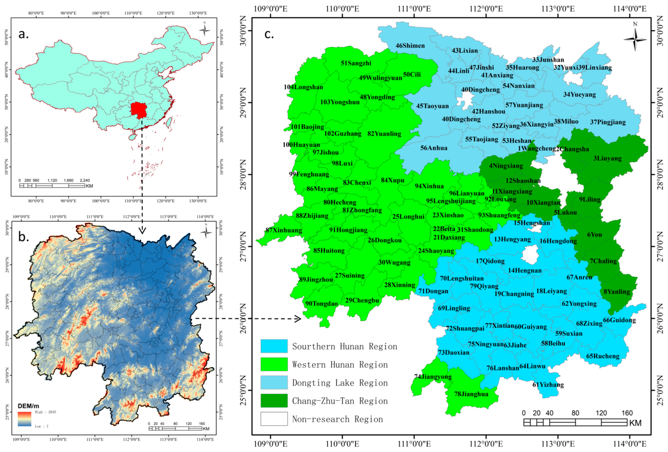
Figure 2.
Average Level of the Agricultural Green Development Index in the Study Region.
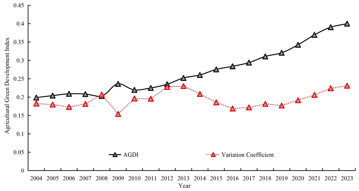
Figure 3.
The Structural Evolution of AGDI in the Study Region.
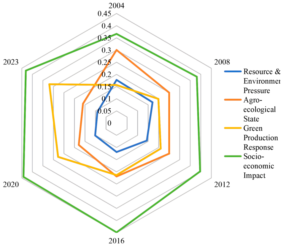
Figure 4.
Spatial Distribution and Evolution of AGD Level in the Study Region.
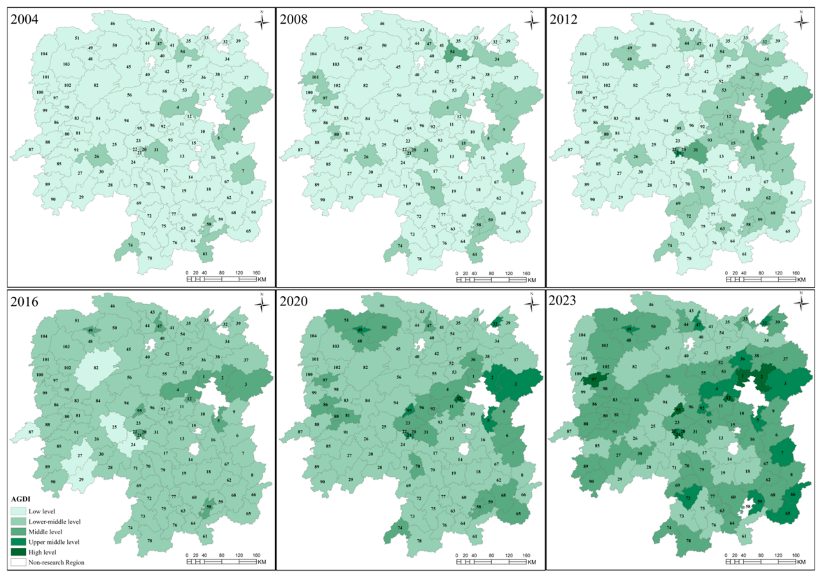

Table 1.
Agricultural Green Development Evaluation Index System.
| Primary Indicator | Secondary Indicators | Unit | Attribute | Weight |
|---|---|---|---|---|
| Resource & Environmental Pressure | Fertilizer Use Intensity | kg·ha⁻¹ | − | 0.07269 |
| Pesticide Use Intensity | kg·ha⁻¹ | − | 0.07406 | |
| Agricultural Film Use Intensity | kg·ha⁻¹ | − | 0.06673 | |
| Agricultural Diesel Oil Use Intensity | kg·ha⁻¹ | − | 0.07143 | |
| Agro-ecological State | Cropping Index | – | + | 0.07862 |
| Forest Coverage Rate | % | + | 0.08086 | |
| Crop Disaster Rate | % | − | 0.08025 | |
| Green Production Response | Soil Erosion Control Level | – | + | 0.08704 |
| Green Food Certification Density | units per 10³ ha | + | 0.08390 | |
| Water-saving Irrigation Coefficient | % | + | 0.08592 | |
| Socio-economic Impact | Rural Per Capita Disposable Income | 10⁴ CNY | + | 0.07117 |
| Urban–Rural Income Ratio | - | − | 0.07430 | |
| Rural Engel Coefficient | % | − | 0.07305 |
Table 2.
Description of the Variables.
| Variables | Acronyms | Description | Unit | Mean | Standard deviation |
Min | Max |
|---|---|---|---|---|---|---|---|
| Agricultural Green Development Index | AGDI | Refer to Section 2.1 | — | 0.2719 | 0.0840 | 0.1204 | 0.6796 |
| Agricultural economic development level | ECO | Primary industry output value / rural population |
CNY /person |
3102.799 | 1301.4140 | 767.9431 | 8041.228 |
| Non-farm employment structure | NFA | Rural non-agricultural employment population /rural population |
% | 0.6755 | 0.0678 | 0.4210 | 0.8493 |
| Agricultural fiscal support | GOV | Expenditure on agriculture, forestry and water affairs / public fiscal expenditure | % | 0.1428 | 0.0624 | 0.0094 | 0.3591 |
| Agricultural service index | SER | Output of agricultural services / total output | % | 0.0300 | 0.0252 | 0.0033 | 0.1252 |
| Agricultural mechanization intensity | MEC | Total power of agricultural machinery / arable land area | kW/ha | 14.1531 | 7.2449 | 2.0653 | 44.5984 |
| Urbanization rate | URB | Urban population / total population | % | 0.4337 | 0.1534 | 0.1125 | 0.9007 |
| Per capita arable land | LAD | Arable land area / rural population | Ha /person |
0.0731 | 0.0205 | 0.0275 | 0.1655 |
Table 3.
Correlation Matrix of the Variables.
| Variable | LNECO | SER | LNMEC | LNGOV | NFA | LNLAD | URB |
| LNECO | 1.000 | ||||||
| SER | 0.249* | 1.000 | |||||
| LNMEC | 0.470* | 0.274* | 1.000 | ||||
| LNGOV | -0.072* | -0.117* | -0.066 | 1.000 | |||
| NFA | 0.304* | 0.169* | 0.428* | -0.158* | 1.000 | ||
| LNLAD | 0.356* | -0.073* | -0.339* | 0.041 | -0.221* | 1.000 | |
| URB | 0.433* | 0.488* | 0.533* | -0.152* | 0.380* | -0.088* | 1.000 |
Note: * indicates significance at the 5% level after Bonferroni correction.
Table 4.
Endogeneity Tests Results.
| Variable | Instrumental variable | F | LM | C-D Wald F |
|---|---|---|---|---|
| LNECO | L.LNECO | 0.0000 | 944.674*** | 1899.890 |
| SER | L.SER | 0.0001 | 1199.046*** | 3322.988 |
| LNMEC | L.LNMEC | 0.0729 | 799.595*** | 1390.561 |
| LNGOV | L.LNGOV | 0.3473 | 884.862*** | 1671.768 |
| NFA | L.NFA | 0.0006 | 810.375*** | 1423.619 |
| URB | L.URB | 0.0199 | 1368.682*** | 5071.528 |
Note: 1. The null hypothesis is that the variable is exogenous. 2. The data corresponding to F-statistic is pvalues of Wu Hausmann F-test.
Table 5.
Estimation Results of the Baseline Panel Models.
| Variable | Model 1 Pooled OLS |
Model 2 | Model 3 | Model 4 |
|---|---|---|---|---|
| FE | LSDV | RE | ||
| LNECO | 0.0307** (0.0122) |
0.0891*** (0.0174) |
0.0891*** (0.0179) |
0.0730*** (0.0140) |
| SER | 0.7223*** (0.1651) |
1.3347*** (0.1810) |
1.3347*** (0.1857) |
1.2111*** (0.1653) |
| LNMEC | 0.0144 (0.0090) |
0.0086 (0.0106) |
0.0086 (0.0109) |
0.0123 (0.0088) |
| LNGOV | -0.0068 (0.0074) |
-0.0048 (0.0091) |
-0.0048 (0.0093) |
-0.0026 (0.0065) |
| NFA | 0.1999*** (0.0492) |
0.3138*** (0.0624) |
0.3138*** (0.0640) |
0.2936*** (0.0514) |
| URB | -0.0202 (0.0174) |
-0.0820*** (0.0226) |
-0.0820*** (0.0232) |
-0.0607*** (0.0195) |
| LNLAD | 0.0019*** (0.0003) |
0.0017*** (0.0006) |
0.0017** (0.0007) |
0.0019*** (0.0005) |
| _cons | -0.3171*** (0.1141) |
-1.0137*** (0.1645) |
-1.0519*** (0.1763) |
-0.8218*** (0.1419) |
| R² | 0.5350 | 0.6831 | 0.7778 | 0.5226 |
Note: 1. Model 1 is pooled regression model, Model 2 and Model 3 are fixed effects models, Model 4 is random effects model. 2. chibar2(01)=2704.66, p=0.0000; χ²(7)=147.35, p=0.0000. 3. Standard errors in parentheses. *p < 0.1, **p < 0.05, ***p < 0.01.
Table 6.
Results of the Threshold Effect Test.
| Threshold | RSS | MSE | F | P | 10% | 5% | 1% |
|---|---|---|---|---|---|---|---|
| Single | 3.0272 | 0.0015 | 134.46 | 0.0160 | 92.8335 | 106.4907 | 144.6647 |
| Double | 2.861 | 0.0015 | 113.74 | 0.0000 | 63.0319 | 74.5494 | 91.1804 |
| Triple | 2.7756 | 0.0014 | 60.19 | 0.9340 | 139.3859 | 153.4614 | 178.1569 |
Table 7.
Threshold Estimation and Confidence Intervals.
| Threshold | Estimate | 95% Confidence Interval | Corresponding ECO (CNY/person) |
|---|---|---|---|
| First threshold (γ1) | 7.5803 | [7.5790, 7.5857] | ≈1959 |
| Second threshold (γ2) | 8.1256 | [8.1200, 8.1278] | ≈3380 |
Table 8.
Panel Threshold Regression Results.
| Variable | L.LNECO ≤ 7.5803 | 7.5803 < L.LNECO ≤ 8.1256 | L.LNECO > 8.1256 |
|---|---|---|---|
| SER | 0.5374 (0.3832) |
1.2203*** (0.2113) |
1.2733*** (0.2540) |
| LNMEC | 0.0389* (0.0213) |
0.0328** (0.0159) |
0.1111*** (0.0192) |
| LNGOV | -0.0072 (0.0110) |
0.0000 (0.0112) |
-0.0085 (0.0109) |
| NFA | 0.4841*** (0.1049) |
0.5445*** (0.1096) |
0.2310** (0.1096) |
| URB | 0.0018** (0.0008) |
||
| LNLAD | -0.0297 (0.0224) |
||
| _cons | -0.3751*** (0.0907) |
||
Note:1. The standard deviations are indicated in parentheses. 2. *p < 0.1,** p < 0.05, ***p < 0.01.
Table 9.
Heterogeneity Analysis Results by Region and Development Stage.
| Panel A: Low Stage(ECO≤1959) | ||||
| Variable | Chang-Zhu-Tan | Dongting Lake | Western Hunan | Southern Hunan |
| SER | — | — | 0.9265* (0.4724) |
— |
| LNMEC | — | — | 0.0140 (0.0178) |
— |
| NFA | — | — | 0.1929* (0.1087) |
— |
| LNGOV | — | — | -0.0282* (0.0143) |
— |
| N | 1 | 13 | 269 | 50 |
| R² | — | — | 0.6178 | — |
| Panel B: Middle Stage(1959<ECO<3380) | ||||
| Variable | Chang-Zhu-Tan | Dongting Lake | West Hunan | South Hunan |
| SER | 1.1913 (0.6835) |
0.7904** (0.2754) |
1.9352*** (0.5780) |
0.9342*** (0.1323) |
| LNMEC | 0.0568** (0.0223) |
0.1250*** (0.0252) |
0.0600** (0.0253) |
-0.0202 (0.0182) |
| NFA | 0.6284 (0.3865) |
-0.3122* (0.1601) |
0.6100*** (0.1912) |
0.2176 (0.1550) |
| LNGOV | 0.0300 (0.0204) |
-0.0639*** (0.0199) |
0.0138 (0.0319) |
0.0040 (0.0115) |
| N | 73 | 112 | 444 | 279 |
| R² | 0.7154 | 0.8677 | 0.6199 | 0.7505 |
| Panel C: High Stage(ECO≥3380) | ||||
| Variable | Chang-Zhu-Tan | Dongting Lake | West Hunan | South Hunan |
| SER | 0.7476 (0.4378) |
1.5610*** (0.4579) |
1.0008 (1.1568) |
0.5903 (0.3488) |
| LNMEC | 0.1510 (0.1000) |
0.1633*** (0.0493) |
0.1634* (0.0816) |
0.2033*** (0.0315) |
| NFA | 0.1961 (0.2361) |
0.0439 (0.1468) |
0.6626** (0.2536) |
0.4504 (0.3425) |
| LNGOV | -0.0203 (0.0195) |
-0.0467* (0.0260) |
0.0501 (0.0660) |
-0.0025 (0.0688) |
| N | 135 | 312 | 104 | 184 |
| R² | 0.7978 | 0.6843 | 0.6599 | 0.7207 |
Note: 1. Results for samples with N < 50 are marked as “—”. 2. The standard deviations are indicated in parentheses. 3. *p < 0.1,** p < 0.05, ***p < 0.01.
Table 10.
Robustness Test Results.
| Variable (regime) | (1) | (2) | (3) | (4) |
|---|---|---|---|---|
| SER (Regime 1) | 0.5374 (0.3832) |
0.5374 (0.3832) |
0.4877 (0.3915) |
0.4688 (0.3855) |
| SER (Regime 2) | 1.2203*** (0.2113) |
1.2203*** (0.2113) |
1.1804*** (0.2074) |
1.1257*** (0.1929) |
| SER (Regime 3) | 1.2733*** (0.2540) |
1.2733*** (0.2540) |
1.2637*** (0.2594) |
1.0354*** (0.2331) |
| LNMEC (Regime 1) | 0.0389* (0.0213) |
0.0389* (0.0213) |
0.0323 (0.0210) |
0.0241 (0.0190) |
| LNMEC (Regime 2) | 0.0328** (0.0159) |
0.0328** (0.0159) |
0.0273 (0.0165) |
0.0326** (0.0152) |
| LNMEC (Regime 3) | 0.1111*** (0.0192) |
0.1111*** (0.0192) |
0.1061*** (0.0194) |
0.1123*** (0.0218) |
| LNGOV (Regime 1) | -0.0072 (0.0110) |
-0.0072 (0.0110) |
-0.0053 (0.0109) |
-0.0038 (0.0115) |
| LNGOV (Regime 2) | 0.0000 (0.0112) |
0.0000 (0.0112) |
0.0022 (0.0115) |
-0.0010 (0.0113) |
| LNGOV (Regime 3) | -0.0085 (0.0109) |
-0.0085 (0.0109) |
-0.0053 (0.0110) |
-0.0098 (0.0117) |
| NFA (Regime 1) | 0.4841*** (0.1049) |
0.4841*** (0.1049) |
0.4917*** (0.1081) |
0.4631*** (0.0989) |
| NFA (Regime 2) | 0.5445*** (0.1096) |
0.5445*** (0.1096) |
0.5494*** (0.1118) |
0.4706*** (0.1092) |
| NFA (Regime 3) | 0.2310** (0.1096) |
0.2310** (0.1096) |
0.2370** (0.1104) |
0.2551** (0.1065) |
| URB | 0.0018** (0.0008) |
0.0018** (0.0008) |
0.0020** (0.0008) |
0.0022*** (0.0007) |
| LNLAD | -0.0297 (0.0224) |
-0.0297 (0.0224) |
-0.0390* (0.0234) |
-0.0706*** (0.0186) |
| _cons | -0.3751*** (0.0907) |
-0.3751*** (0.0907) |
-0.3913*** (0.0921) |
-0.4218*** (0.0916) |
| R² | 0.6998 | 0.6998 | 0.6986 | 0.7049 |
| Threshold Values | 7.5803; 8.1256 | 7.5803; 8.1256 | 7.5803; 8.1256 | 7.5914; 8.1217 |
Note: 1. Column (1) is Benchmark; Column (2) increases the number of bootstrap replications to 1000; Column (3) re-estimates the model after 1% two-sided winsorization of continuous variables; Column (4) replaces the mechanization measure with the ratio of total agricultural machinery power to sown area. 2. Standard errors in parentheses; 3. *p < 0.1,** p < 0.05, ***p < 0.01.
Disclaimer/Publisher’s Note: The statements, opinions and data contained in all publications are solely those of the individual author(s) and contributor(s) and not of MDPI and/or the editor(s). MDPI and/or the editor(s) disclaim responsibility for any injury to people or property resulting from any ideas, methods, instructions or products referred to in the content. |
© 2026 by the authors. Licensee MDPI, Basel, Switzerland. This article is an open access article distributed under the terms and conditions of the Creative Commons Attribution (CC BY) license.
Copyright: This open access article is published under a Creative Commons CC BY 4.0 license, which permit the free download, distribution, and reuse, provided that the author and preprint are cited in any reuse.