Hodge Atoms and Intersection Spaces at Conifold Degenerations

1. Introduction

Degenerations of smooth projective varieties provide a natural setting in which smooth geometry, singular topology, monodromy, and Hodge theory meet. For a projective one-parameter degeneration $\pi :\mathcal{X}\to \Delta$, the cohomology of a smooth fiber $X_t:={\pi }^{-1}\left(t\right)$, $t\ne 0$, is related to the singular central fiber $X_0:={\pi }^{-1}\left(0\right)$ through nearby and vanishing cycles. In Saito’s mixed-Hodge-module formalism, these functors carry the limiting mixed Hodge structure together with the canonical and variation morphisms and the nilpotent logarithm of unipotent monodromy [1,2,3]. For isolated hypersurface singularities, and in particular for ordinary double points, the local contribution is described by Milnor-fiber topology and classical Picard–Lefschetz theory [4,5]. On the singular fiber, intersection cohomology provides a canonical pure intersection-complex realization, while the intersection-space construction provides a different singular-space theory designed to retain smoothing-type information. The corresponding perverse-sheaf specialization theory was developed by Banagl–Budur–Maxim [6].

The present paper studies the interaction of these structures for finite-node threefold degenerations. Throughout the degeneration-side analysis, we work with a projective morphism $\pi :\mathcal{X}\to \Delta$ satisfying Definition 1: the total space $\mathcal{X}$ is a smooth complex fourfold, each fiber $X_t$ with $t\ne 0$ is a smooth projective threefold, and the central fiber $X_0$ has finite singular locus $\Sigma =\{p_1,\dots ,p_r\}$, with every $p_a$ an ordinary double point. The results of Section 2, Section 3 and Section 4, together with the $IC$–intersection-space defect calculation of Section 6, use this finite-node threefold setup and the intersection-space mixed-Hodge-module realization and specialization assumptions stated in Section 2.4. The additional assumption that the smooth fibers $X_t$ are Calabi–Yau threefolds is imposed in Section 5, where the weight sectors are compared with the Hodge-atom and F-bundle structures of [7], and in the classical 125-node quintic application of Section 6.3.

The present paper is a direct continuation of the defect-triangle framework developed in [8]. That work introduced a mixed-Hodge-module architecture for comparing nearby and vanishing cycles with the intersection-space realization of a singular fiber while keeping several potentially distinct defect mechanisms separate. In the normalization used here, set $F:={\mathbb{Q}}_{\mathcal{X}}^H\left[4\right]$, and write $\Psi :={\psi }_{\pi ,1}^p\left(F\right)$ and $\Phi :={\varphi }_{\pi ,1}^p\left(F\right)$ for the perverse-normalized unipotent nearby- and vanishing-cycle mixed Hodge modules. Saito’s nearby–vanishing formalism provides the canonical morphism $\mathrm{can}:\Psi \to \Phi$ and the variation morphism $\mathrm{var}:\Phi \to \Psi (-1)$ in $\mathrm{MHM}\left(X_0\right)$, where $(-1)$ denotes the Tate twist [2,3]. The defect-triangle construction combines these nearby–vanishing data with a mixed-Hodge-module realization ${\mathcal{IS}}_{X_0}^H\in \mathrm{MHM}\left(X_0\right)$ of the Banagl–Budur–Maxim intersection-space perverse sheaf [6,8]. The present paper evaluates that framework in the threefold ordinary-double-point regime and determines which of its defect terms survive, which collapse, and how the surviving carrier is organized by global vanishing relations, monodromy, and the limiting weight filtration.

Under the specialization assumption used in [8], the nearby carrier admits the schematic splitting

$$\Psi \simeq {\mathcal{IS}}_{X_0}^H\oplus {\mathcal{C}}_{\Sigma }^H,$$

where ${\mathcal{C}}_{\Sigma }^H$ denotes the singularity-supported specialization complement. Let ${\mathrm{pr}}_I:\Psi \to {\mathcal{IS}}_{X_0}^H$ be the projection associated with this splitting. The projected variation morphism is ${\mathrm{var}}_I:={\mathrm{pr}}_I(-1)\circ \mathrm{var}$, with projected shifted variation carrier $P_I^H:=\mathrm{Cone}\left({\mathrm{var}}_I\right)[-1]$. The unprojected shifted variation carrier is $P_{\mathrm{var}}^H:=\mathrm{Cone}\left(\mathrm{var}\right)[-1]$. The octahedral comparison of [8] then gives the distinguished triangle

$$P_{\mathrm{var}}^H⟶P_I^H⟶{\mathcal{C}}_{\Sigma }^H(-1)\stackrel{+1}{\to }.$$

The purpose of this triangle is to keep several a priori distinct phenomena separate: the failure of the intersection-space summand to exhaust nearby cycles, global dependencies among nodewise vanishing directions, and the difference between intersection-space and intersection-complex realizations. No equality among these defect mechanisms was assumed in advance [8].

This formulation leaves a concrete question. In the ordinary-double-point threefold regime relevant to Calabi–Yau conifold degenerations, is the specialization complement ${\mathcal{C}}_{\Sigma }^H$ actually nonzero? If it vanishes, what geometric information remains inside the surviving intersection-space carrier? A second question, motivated by [7], is whether the rigid–flexible Hodge-atom structure at a conifold degeneration can be located intrinsically within the limiting mixed Hodge structure rather than only compared with it after passage to the smooth-side analytic theory. These questions provide the starting point of the present paper.

The first question has a particularly rigid answer. Let $F_a$ denote the Milnor fiber at $p_a$. For a threefold ordinary double point, $F_a\simeq S^3$ up to homotopy, and therefore ${\tilde{H}}^3(F_a;\mathbb{Q})$ is one-dimensional [4]. If $T_a$ denotes the local Milnor monodromy on this vanishing cohomology, the Picard–Lefschetz formula and the skew-symmetry of the middle intersection pairing in odd dimension give $T_a=\mathrm{id}$ [4,5]. The Banagl–Budur–Maxim specialization theorem identifies the complementary term with the contribution of the local $T-\mathrm{id}$ image; trivial local monodromy therefore forces this contribution to vanish ([6], Theorem 3.2(c), Remark 3.3(i)–(ii)). Under the finite-node mixed-Hodge-module globalization assumption described in Section 2.4, we prove in Theorem 1 that

$${\mathcal{C}}_{\Sigma }^H=0,{\mathcal{IS}}_{X_0}^H\simeq \Psi .$$

Consequently $P_{\mathrm{var}}^H\simeq P_I^H$, and the projected defect triangle collapses in the ordinary-double-point specialization.

This collapse does not exhaust the defect geometry; rather, it changes the form of the problem. Once the intersection-space mixed Hodge module is identified with nearby cycles, the relevant structures are no longer external complements of ${\mathcal{IS}}_{X_0}^H$, but internal structures of the common carrier $\Psi \simeq {\mathcal{IS}}_{X_0}^H$. The paper therefore turns to three questions: which combinations of the r formal nodewise vanishing directions survive globally, how the surviving classes are encoded by nilpotent monodromy, and how this information is distributed through the weight filtration $W_{•}\Psi$ supplied by Saito’s nearby cycle theory [2,3].

To formulate the first question, let $e_1,\dots ,e_r$ be the standard basis of ${\mathbb{Q}}^r$, and let ${\delta }_a\in H^3(X_t,\mathbb{Q})$ denote the global vanishing class associated with $p_a$. The Picard–Lefschetz realization map is

$${\rho }_{\mathrm{van}}:{\mathbb{Q}}^r⟶H^3(X_t,\mathbb{Q}),e_a⟼{\delta }_a.$$

Define the global relation space $R_{\mathrm{van}}:=\ker \left({\rho }_{\mathrm{van}}\right)$, write $\delta :={\dim }_{\mathbb{Q}}{R}_{\mathrm{van}}$, and set $V_{\mathrm{glob}}:=\mathrm{im}\left({\rho }_{\mathrm{van}}\right)=\langle {\delta }_1,\dots ,{\delta }_r\rangle$. Thus ${\dim }_{\mathbb{Q}}{V}_{\mathrm{glob}}=r-\delta$. Under proper nearby-cycle comparison, the hypercohomology of the variation morphism realizes this Picard–Lefschetz map; this is the standard nearby–vanishing-cycle interpretation of variation ([5], §4.2) and its mixed-Hodge-theoretic degeneration interpretation is discussed in [9]. In Theorem 2 and Corollary 2, we show that the corresponding mixed-Hodge relation object is $R_{\mathrm{van}}^H\simeq {\mathbb{Q}}^H{(-2)}^{\oplus \delta }$.

The same geometry controls global monodromy. Let $T_u$ denote the unipotent part of global monodromy and $N:={\left(2\pi i\right)}^{-1}\log T_u$ its nilpotent logarithm. The identity $N=\mathrm{var}\circ \mathrm{can}$ is part of Saito’s nearby–vanishing formalism [2,3]. The global Picard–Lefschetz calculation of Theorem 3 gives

$$\mathrm{im}N=V_{\mathrm{glob}},N^2=0,\ker N=V_{\mathrm{glob}}^{\perp }.$$

These identities are classical Picard–Lefschetz consequences in the finite-node setting. Their role here is to place the globally surviving vanishing sector inside the monodromy-weight structure of the common intersection-space/nearby carrier.

The principal structural result is the corresponding description at the mixed-Hodge-module level. Let $i_a:\left\{p_a\right\}\hookrightarrow X_0$ denote the inclusion of the a-th node, and define

$$K:=\ker \left({\mathbb{Q}}_{X_0}^H\left[3\right]⟶I{C}_{X_0}^H\right).$$

For an ordinary double point, the local link calculation together with Saito’s weight formalism gives $K\simeq {⨁}_{a=1}^r{\left(i_a\right)}_{*}{\mathbb{Q}}_{\left\{p_a\right\}}^H(-1)$, whereas the vanishing-cycle module is $\Phi \simeq {⨁}_{a=1}^r{\left(i_a\right)}_{*}{\mathbb{Q}}_{\left\{p_a\right\}}^H(-2)$ [3,4]. We prove in Theorem 4 that $\Psi \simeq {\mathcal{IS}}_{X_0}^H$ carries the weight filtration

$$0\subset W_2\Psi \subset W_3\Psi \subset W_4\Psi =\Psi$$

with

$${\mathrm{Gr}}_2^W\Psi \simeq K,{\mathrm{Gr}}_3^W\Psi \simeq I{C}_{X_0}^H,{\mathrm{Gr}}_4^W\Psi \simeq \Phi ,$$

and with nilpotent monodromy inducing $N:{\mathrm{Gr}}_4^W\Psi \stackrel{\sim }{\to }{\mathrm{Gr}}_2^W\Psi (-1)$. After hypercohomology, Section 4.4 identifies the pure middle piece as ${\mathrm{Gr}}_3^W{H}_{\lim }^3\simeq I{H}^3(X_0,\mathbb{Q})$. Intersection cohomology therefore appears as the pure weight-three component of the full nearby/intersection-space realization.

The weight filtration also determines the $IC$–intersection-space defect. In $K_0\left(\mathrm{MHM}\left(X_0\right)\right)$, define ${\Delta }_{I/IC}\left(X_0\right):=\left[{\mathcal{IS}}_{X_0}^H\right]-\left[I{C}_{X_0}^H\right]$. The two canonical short exact sequences underlying the weight filtration give, in Theorem 6,

$${\Delta }_{I/IC}\left(X_0\right)=[\Phi ]+\left[K\right].$$

The specialization complement, the global relation object, and the $IC$–intersection-space Grothendieck defect are therefore categorically different constructions. The first vanishes in the present ordinary-double-point regime; the second measures dependencies among the local vanishing directions; and the third records the two point-supported Tate layers surrounding the pure intersection-complex core. Their numerical interaction emerges only after globalization: by Proposition 6, both outer pieces of the limiting middle cohomology have dimension $r-\delta$.

When the finite-node degeneration is moreover a Calabi–Yau conifold degeneration, the preceding weight-filtration results admit the Hodge-atom interpretation developed in [7]. In that work, the degeneration-side Hodge-atom carrier is defined by the unshifted variation cone

$$P_{\mathrm{atom}}^H:=\mathrm{Cone}\left(\mathrm{var}:\Phi \to \Psi (-1)\right).$$

This differs by one cohomological shift from the variation carrier used in the defect-triangle formalism, $P_{\mathrm{var}}^H=\mathrm{Cone}\left(\mathrm{var}\right)[-1]$, and hence $P_{\mathrm{atom}}^H\simeq P_{\mathrm{var}}^H\left[1\right]$. Using the weight filtration established in Section 4.3, we prove in Theorem 5 that

$$P_{\mathrm{atom}}^H\simeq (\Psi /W_2\Psi )(-1).$$

After accounting for this fixed Tate normalization, the degeneration-side Hodge-atom carrier is therefore the quotient of the full nearby/intersection-space carrier by its weight-two subobject. Its rigid contribution is carried by the pure weight-three sector, while its degeneration-side flexible contribution is carried by the upper weight-four sector. The full nearby realization contains in addition the lower weight-two flexible sector, and nilpotent monodromy identifies the two outer sectors up to Tate twist. Thus the Hodge-atom carrier and the full nearby carrier are distinct but canonically related realizations of the same degeneration geometry.

The classical 125-node quintic provides a numerical realization of the entire structure. For the Schoen quintic, $r=125$, while the classical conifold-transition calculation gives relation rank $\delta =24$ and global vanishing rank $r-\delta =101$ [10,11,12]. A nearby smooth quintic has $b_3\left(X_t\right)=204$, whereas the pure intersection-cohomology contribution has dimension 2. Section 6.3 therefore yields the weight profile

$$204=101+2+101.$$

The degeneration-side Hodge-atom quotient has middle rank $103=2+101$, whereas the full nearby/intersection-space realization contains the additional lower flexible sector of rank 101. Equivalently, the rank-202 difference between the full middle nearby/intersection-space realization and its pure intersection-cohomology core is $202=2(125-24)$.

Taken together, these results provide a single geometric framework for structures arising at different stages of a nodal degeneration. Local ordinary double points furnish formal vanishing directions; global relations determine which combinations survive; nilpotent monodromy places the surviving quotient inside the limiting mixed Hodge structure; the intersection-space mixed Hodge module realizes the full nearby carrier; intersection cohomology appears as its pure weight-three core; and, in the Calabi–Yau conifold setting, the Hodge-atom carrier is obtained from its weight-three/weight-four quotient. The resulting separation of local existence, global survival, pure singular geometry, and full nearby realization is the principal conceptual organization supplied by the paper.

1.1. Mixed-Hodge-Module Conventions

We briefly collect the normalization used throughout the paper. With $F={\mathbb{Q}}_{\mathcal{X}}^H\left[4\right]$, the perverse-normalized unipotent nearby and vanishing cycles are $\Psi ={\psi }_{\pi ,1}^p\left(F\right)$ and $\Phi ={\varphi }_{\pi ,1}^p\left(F\right)$. The canonical and variation morphisms are $\mathrm{can}:\Psi \to \Phi$ and $\mathrm{var}:\Phi \to \Psi (-1)$, and Saito’s identities give

$$\mathrm{var}\circ \mathrm{can}=N_{\Psi },\mathrm{can}(-1)\circ \mathrm{var}=N_{\Phi }$$

References [2,3]. All Tate twists are retained explicitly in weight- and duality-sensitive statements.

For a threefold ordinary double point, the reduced Milnor cohomology is one-dimensional in degree three and the corresponding vanishing-cycle mixed Hodge structure is ${\mathbb{Q}}^H(-2)$. Consequently,

$$\Phi \simeq {\displaystyle \underset{a=1}{\overset{r}{⨁}}}{\left(i_a\right)}_{*}{\mathbb{Q}}_{\left\{p_a\right\}}^H(-2),{\mathbb{H}}^0(X_0;\Phi )\simeq {\mathbb{Q}}^H{(-2)}^{\oplus r},$$

with all other hypercohomology groups of the point-supported object $\Phi$ equal to zero. Thus ${\mathbb{H}}^0(X_0;\Phi )$ is the formal mixed-Hodge space generated by the nodewise vanishing directions.

1.2. Principal Results

We summarize the principal conclusions, referring to the body of the paper for the precise statements, assumptions, and proofs.

Intersection-space realization. The local calculation of Section 2.3, together with the Banagl–Budur–Maxim specialization theorem ([6], Theorem 3.2(c), Remark 3.3(i)–(ii)), gives

$${\mathcal{C}}_{\Sigma }^H=0,{\mathcal{IS}}_{X_0}^H\simeq \Psi$$

under the realization and specialization assumptions of Section 2.4; see Theorem 1.

Global relation realization. The variation morphism determines the relation object

$$R_{\mathrm{van}}^H:=\ker \left[{\mathbb{H}}^0(X_0;\Phi )⟶{\mathbb{H}}^0(X_0;{\mathcal{IS}}_{X_0}^H)(-1)\right],$$

whose underlying rational space is $R_{\mathrm{van}}=\ker \left({\rho }_{\mathrm{van}}\right)$. If $\delta ={\dim }_{\mathbb{Q}}{R}_{\mathrm{van}}$, then $R_{\mathrm{van}}^H\simeq {\mathbb{Q}}^H{(-2)}^{\oplus \delta }$, and the globally realized vanishing sector has dimension $r-\delta$; see Theorem 2 and Corollary 2.

Monodromy and weight filtration. Theorem 3 gives

$$\mathrm{im}N=V_{\mathrm{glob}},N^2=0,\ker N=V_{\mathrm{glob}}^{\perp }.$$

Theorem 4 identifies the weight filtration of the common nearby/intersection-space carrier as $0\subset W_2\Psi \subset W_3\Psi \subset W_4\Psi =\Psi$, with

$${\mathrm{Gr}}_2^W\Psi \simeq K,{\mathrm{Gr}}_3^W\Psi \simeq I{C}_{X_0}^H,{\mathrm{Gr}}_4^W\Psi \simeq \Phi .$$

Theorem 6 then gives ${\Delta }_{I/IC}\left(X_0\right)=[\Phi ]+\left[K\right]$, while Proposition 6 yields

$$b_3\left(X_t\right)=2(r-\delta )+\dim I{H}^3(X_0,\mathbb{Q}).$$

Hodge-atom realization. For a finite-node Calabi–Yau conifold degeneration, Theorem 5 gives

$$P_{\mathrm{atom}}^H\simeq (\Psi /W_2\Psi )(-1).$$

After the fixed Tate normalization is accounted for, its rigid Hodge-atom sector is carried by ${\mathrm{Gr}}_3^W\Psi$, its degeneration-side flexible sector by ${\mathrm{Gr}}_4^W\Psi$, and the full nearby realization contains the additional monodromy-dual flexible sector ${\mathrm{Gr}}_2^W\Psi$. Both outer sectors have rank $r-\delta$.

The common feature of these results is that the weight filtration of nearby cycles becomes the organizing structure relating intersection spaces, intersection cohomology, global vanishing-cycle relations, monodromy, and the Hodge-atom decomposition.

1.3. Scope and Organization

Section 2, Section 3 and Section 4 develop the degeneration-side mixed-Hodge-module theory for finite-node projective threefold degenerations with smooth total space under the realization and specialization assumptions stated in Section 2.4. Section 5 adds the assumption that the smooth fibers are Calabi–Yau threefolds and compares the resulting weight sectors with the Hodge-atom and F-bundle structures of [7]. Section 6 returns to the $IC$–intersection-space defect and gives the principal nodal-quintic application.

More precisely, Section 2 fixes the nearby–vanishing conventions, computes the ordinary-double-point vanishing module, evaluates the Banagl–Budur–Maxim specialization complement, and proves ${\mathcal{IS}}_{X_0}^H\simeq \Psi$. Section 3 identifies the global relation object and the globally realized vanishing sector and determines their Picard–Lefschetz monodromy structure. Section 4 determines the sheaf-level weight filtration of the common nearby/intersection-space carrier and identifies its pure middle graded piece with $I{C}_{X_0}^H$. Section 5 identifies the unshifted Hodge-atom carrier with $(\Psi /W_2\Psi )(-1)$ and describes the rigid and two flexible weight sectors. Section 6 derives the $IC$–intersection-space Grothendieck defect, determines the global ranks of the outer weight pieces, and analyzes the classical 125-node quintic. Finally, Section 7 treats integral fidelity, characteristic-class and motivic refinements, extensions beyond ordinary double points, BPS/Donaldson–Thomas interfaces, and the concluding perspective.

Appendix A records the normalization, weight, duality, and coefficient conventions needed to audit the main arguments. Appendix B records the broader catalog of extension mechanisms that collapse in the present ordinary-double-point specialization but become nontrivial again beyond this regime.

2. Conifold Geometry, Nearby Cycles, and Defect Data

This section fixes the geometric and mixed-Hodge-module framework used throughout the degeneration-side analysis. We work with projective one-parameter degenerations whose total space is smooth, whose general fiber is a smooth projective threefold, and whose central fiber has only finitely many ordinary double points. No assumption that the smooth fibers are Calabi–Yau is made in Section 2, Section 3 and Section 4; the Calabi–Yau assumption enters only in the Hodge-atom and F-bundle comparison of Section 5.

The principal inputs are Saito’s perverse-normalized nearby- and vanishing-cycle formalism [1,2,3] and the intersection-space specialization theorem of Banagl–Budur–Maxim [6]. The ordinary-double-point calculation has a particularly strong consequence: the local Milnor monodromy acts trivially on the rank-one vanishing cohomology, so the Banagl–Budur–Maxim specialization complement vanishes. Under the mixed-Hodge-module realization and globalization assumptions stated in Section 2.4, the intersection-space mixed Hodge module therefore coincides with the unipotent nearby-cycle carrier.

This result simplifies the defect-triangle architecture of [8]. In the ordinary-double-point threefold regime, the projected canonical and variation carriers collapse to their unprojected counterparts. The global vanishing-cycle relations, the $IC$–intersection-space defect, and the integral extension defects, however, remain distinct structures and need not vanish.

2.1. Finite-Node Threefold Degenerations

Definition 1 

(Finite-node threefold degeneration). Let $\Delta \subset \mathbf{C}$ be a sufficiently small analytic disc centered at 0, and let $\pi :\mathcal{X}\to \Delta$ be a proper projective morphism from a smooth complex fourfold. For $t\in \Delta$, write $X_t:={\pi }^{-1}\left(t\right)$. We call π a finite-node threefold degeneration if π is smooth over ${\Delta }^{\times }:=\Delta \setminus \left\{0\right\}$, every $X_t$ with $t\ne 0$ is a smooth projective threefold, and the central fiber $X_0$ has finite singular locus $\Sigma =\{p_1,\dots ,p_r\}$, with every $p_a$ an ordinary double point. Analytically near $p_a$, the central fiber is locally isomorphic to the hypersurface

$$z_1^2+z_2^2+z_3^2+z_4^2=0in{\mathbf{C}}^4.$$

A finite-node Calabi–Yau conifold degeneration is a finite-node threefold degeneration for which the smooth fibers $X_t$, $t\ne 0$, are Calabi–Yau threefolds.

Write $U:=X_0\setminus \Sigma$, with inclusions $j:U\hookrightarrow X_0$, $i:\Sigma \hookrightarrow X_0$, and $i_a:\left\{p_a\right\}\hookrightarrow X_0$. Since ${\dim }_{\mathbf{C}}{X}_0=3$, the normalized intersection-complex Hodge module $I{C}_{X_0}^H$ is characterized by $j^{*}I{C}_{X_0}^H\simeq {\mathbb{Q}}_U^H\left[3\right]$. On a smooth fiber, the corresponding pure Hodge module is ${\mathbb{Q}}_{X_t}^H\left[3\right]$.

2.2. Nearby and Vanishing Cycles

Since ${\dim }_{\mathbf{C}}\mathcal{X}=4$, set $F:={\mathbb{Q}}_{\mathcal{X}}^H\left[4\right]$. We write $\Psi :={\psi }_{\pi ,1}^p\left(F\right)$ and $\Phi :={\varphi }_{\pi ,1}^p\left(F\right)$ for the perverse-normalized unipotent nearby- and vanishing-cycle mixed Hodge modules. Thus $\Psi ,\Phi \in \mathrm{MHM}\left(X_0\right)$, with ${}^p\psi _{\pi ,1}={\psi }_{\pi ,1}[-1]$ and ${}^p\varphi _{\pi ,1}={\varphi }_{\pi ,1}[-1]$ [1,2,3].

For comparison with the Banagl–Budur–Maxim specialization theorem, let ${\Psi }_{\mathrm{full}}$ denote the full perverse-normalized nearby-cycle object before decomposition into generalized monodromy eigenspaces. The object $\Psi$ is its generalized eigenvalue-1, equivalently unipotent, summand.

For a threefold ordinary double point, the Milnor fiber has the homotopy type of $S^3$ [4]. Its reduced middle cohomology is one-dimensional. With the Tate normalization used throughout this paper, the associated vanishing-cycle mixed Hodge structure is ${\mathbb{Q}}^H(-2)$. Since $\Phi$ is supported on the finite singular set, one obtains

$$\Phi \simeq {\displaystyle \underset{a=1}{\overset{r}{⨁}}}{\left(i_a\right)}_{*}{\mathbb{Q}}_{\left\{p_a\right\}}^H(-2).$$

Proposition 1 

(Ordinary-double-point vanishing module). For a finite-node threefold degeneration,

$${\mathbb{H}}^0(X_0;\Phi )\simeq {\mathbb{Q}}^H{(-2)}^{\oplus r},{\mathbb{H}}^k(X_0;\Phi )=0fork\ne 0.$$

Proof. 

Vanishing cycles vanish on U, so $\Phi$ is supported on the finite closed subset $\Sigma$. By Kashiwara equivalence, a mixed Hodge module supported on $\Sigma$ is equivalent to a finite direct sum of mixed Hodge structures supported at the individual points. The Milnor-fiber calculation at a threefold ordinary double point identifies each local summand with ${\mathbb{Q}}^H(-2)$. Since point-supported mixed Hodge modules have hypercohomology concentrated in degree 0, the result follows. □

Remark 1 

(Vanishing module versus corrected-extension quotient). The Tate structure ${\mathbb{Q}}^H(-2)$ is the actual vanishing-cycle mixed Hodge structure appearing in Φ. It should not be confused with the ${\mathbb{Q}}^H(-1)$-type point-supported correction terms arising in the constant-to-intersection-complex comparison. Those terms occur below as the weight-two kernel of the canonical morphism ${\mathbb{Q}}_{X_0}^H\left[3\right]\to I{C}_{X_0}^H$; see Section 4.2.

2.3. Local Monodromy at a Threefold Ordinary Double Point

Let $F_a$ denote the Milnor fiber at $p_a$, and choose a vanishing generator ${\delta }_a$ so that ${\tilde{H}}^3(F_a;\mathbb{Q})=\mathbb{Q}{\delta }_a$.

Proposition 2 

(Trivial local Milnor monodromy). For every ordinary double point of a finite-node threefold degeneration, the local Milnor monodromy satisfies

$$T_a=\mathrm{id}on{\tilde{H}}^3(F_a;\mathbb{Q}).$$

In particular, the local nearby- and vanishing-cycle contributions have no generalized monodromy eigenspaces with eigenvalue different from 1.

Proof. 

The Picard–Lefschetz formula gives

$$T_a\left({\delta }_a\right)={\delta }_a\pm \langle {\delta }_a,{\delta }_a\rangle {\delta }_a.$$

The middle intersection form in odd dimension is skew-symmetric, hence $\langle {\delta }_a,{\delta }_a\rangle =0$. Therefore $T_a\left({\delta }_a\right)={\delta }_a$. Since ${\tilde{H}}^3(F_a;\mathbb{Q})$ is generated by ${\delta }_a$, the local monodromy is the identity [4,5]. □

Proposition 2 is a local statement and should not be confused with triviality of the global Picard–Lefschetz transformation on $H^3(X_t,\mathbb{Q})$. The global transformation can act nontrivially on classes that pair with the vanishing cycles; this distinction is developed in Section 3.

2.4. The Banagl–Budur–Maxim Specialization Complement

For a projective hypersurface with an isolated singular point, Banagl–Budur–Maxim prove that, under the relevant semisimplicity assumption at the eigenvalue 1, the nearby-cycle perverse sheaf splits into an intersection-space summand and a singularity-supported complement ([6], Theorem 3.2(c)). In their notation this has the form

$${\psi }_{\pi }{\mathbb{Q}}_{\tilde{X}}\left[n\right]\simeq {\mathcal{IS}}_X\oplus \mathcal{C}.$$

The complementary summand is controlled by the local $(T-\mathrm{id})$-contribution, and ([6], Remark 3.3(i)) states explicitly that trivial local monodromy forces $\mathcal{C}\simeq 0$. Their Remark 3.3(ii) records the corresponding extension to finitely many isolated singular points.

The global central fiber considered here need not be presented globally as a hypersurface in projective space. The Banagl–Budur–Maxim result is used locally at each node, where the singularity is an isolated weighted-homogeneous hypersurface singularity. We therefore impose, as in [8], the additional global assumption that the finite-node intersection-space perverse sheaf admits a compatible mixed-Hodge-module realization ${\mathcal{IS}}_{X_0}^H$ and that the local specialization splittings globalize to the corresponding mixed-Hodge-module splitting. This is the finite-node mixed-Hodge-module realization and specialization assumption used below.

Theorem 1 

(Intersection-space realization of nearby cycles). Assume the finite-node mixed-Hodge-module realization and specialization assumption just stated. If every singularity of $X_0$ is an ordinary double point, then ${\mathcal{C}}_{\Sigma }^H=0$. Moreover, the full nearby-cycle object has only the generalized eigenvalue-1 contribution, and hence

$${\Psi }_{\mathrm{full}}\simeq \Psi \simeq {\mathcal{IS}}_{X_0}^H.$$

Proof. 

At the rational perverse-sheaf level, the Banagl–Budur–Maxim specialization complement is the direct sum of the local contributions

$${\displaystyle \underset{a=1}{\overset{r}{⨁}}}{\left(i_a\right)}_{*}\mathrm{Im}\left(T_a-\mathrm{id}:H^3(F_a;\mathbb{Q})⟶H^3(F_a;\mathbb{Q})\right)$$

Reference ([6], Theorem 3.2(c), Remark 3.3(i)–(ii)). By Proposition 2, $T_a=\mathrm{id}$ on $H^3(F_a;\mathbb{Q})$ for every node, so all local complementary summands vanish. The assumed mixed-Hodge-module globalization therefore gives ${\mathcal{C}}_{\Sigma }^H=0$.

The same local calculation shows that no generalized eigenspace with eigenvalue different from 1 occurs in the local nearby cycles. Consequently ${\Psi }_{\mathrm{full}}\simeq \Psi$, and the specialization splitting reduces to $\Psi \simeq {\mathcal{IS}}_{X_0}^H$. □

Remark 2 

(Specialization defect versus other defects). Theorem 1 evaluates only the Banagl–Budur–Maxim specialization complement. It does not imply that the global relations among vanishing cycles vanish, nor does it identify ${\mathcal{IS}}_{X_0}^H$ with $I{C}_{X_0}^H$. The former are determined in Section 3; the latter distinction is described by the weight filtration of Section 4 and the $IC$–intersection-space defect of Section 6.

2.5. Canonical, Variation, and Nilpotent Monodromy

Saito’s unipotent nearby–vanishing formalism provides morphisms $\mathrm{can}:\Psi \to \Phi$ and $\mathrm{var}:\Phi \to \Psi (-1)$ [2,3]. Let $N_{\Psi }:\Psi \to \Psi (-1)$ and $N_{\Phi }:\Phi \to \Phi (-1)$ denote the corresponding nilpotent monodromy morphisms.

Proposition 3 

(Canonical–variation identities). With the Tate twists retained,

$$\mathrm{var}\circ \mathrm{can}=N_{\Psi },\mathrm{can}(-1)\circ \mathrm{var}=N_{\Phi }.$$

Proof. 

These are the canonical–variation identities in Saito’s unipotent nearby-cycle formalism [2,3]. □

On the underlying rational local system, the nilpotent logarithm is $N={\left(2\pi i\right)}^{-1}\log T_u$, where $T_u$ is the unipotent part of monodromy. We do not use $T_u-\mathrm{id}$ as a morphism to a Tate twist in $\mathrm{MHM}\left(X_0\right)$; weight-sensitive statements are formulated using N.

Define the shifted variation and canonical carriers by

$$P_{\mathrm{var}}^H:=\mathrm{Cone}\left(\mathrm{var}:\Phi \to \Psi (-1)\right)[-1],P_{\mathrm{can}}^H:=\mathrm{Cone}\left(\mathrm{can}:\Psi \to \Phi \right)[-1].$$

By Theorem 1, either definition may be written with ${\mathcal{IS}}_{X_0}^H$ in place of $\Psi$.

2.6. Collapse of the Projected Defect in the ODP Specialization

The projected carriers introduced in [8] remain useful for the more general defect architecture. Given a splitting $\Psi \simeq {\mathcal{IS}}_{X_0}^H\oplus {\mathcal{C}}_{\Sigma }^H$, the projected variation and canonical morphisms determine $P_I^H:=\mathrm{Cone}\left({\mathrm{var}}_I\right)[-1]$ and $Q_I^H:=\mathrm{Cone}\left({\mathrm{can}}_I\right)[-1]$.

In the ordinary-double-point regime, Theorem 1 gives ${\mathcal{C}}_{\Sigma }^H=0$, so the splitting has no nontrivial complementary summand.

Corollary 1 

(Collapse of the projected carriers). Under the assumptions of Theorem 1,

$$P_I^H\simeq P_{\mathrm{var}}^H,Q_I^H\simeq P_{\mathrm{can}}^H.$$

Moreover, the defect triangle of [8] reduces to

$$P_{\mathrm{var}}^H\stackrel{\sim }{\to }{P}_I^H⟶0\stackrel{+1}{\to }.$$

Thus the projected carriers contain no additional information in the finite-node threefold ordinary-double-point regime. Their distinction becomes substantive again for singularities for which the Banagl–Budur–Maxim specialization complement is nonzero; see Section 7.4.

2.7. Duality

The present paper retains the Tate twists that were suppressed in some schematic rational-level formulas of [8]. Writing $\mathbb{D}:={\mathbb{D}}_{X_0}$ for Verdier duality, the normalizations used here give

$$\mathbb{D}I{C}_{X_0}^H\simeq I{C}_{X_0}^H\left(3\right),\mathbb{D}\Psi \simeq \Psi \left(3\right),\mathbb{D}\Phi \simeq \Phi \left(4\right).$$

Since ${\mathcal{IS}}_{X_0}^H\simeq \Psi$, one also has $\mathbb{D}{\mathcal{IS}}_{X_0}^H\simeq {\mathcal{IS}}_{X_0}^H\left(3\right)$.

With the cone conventions of Section 2.5, canonical and variation are exchanged by Verdier duality up to the indicated Tate twist and cohomological shift:

$$\mathbb{D}{P}_{\mathrm{can}}^H\simeq P_{\mathrm{var}}^H\left(4\right)\left[1\right],\mathbb{D}{P}_{\mathrm{var}}^H\simeq P_{\mathrm{can}}^H\left(4\right)\left[1\right].$$

These identities exhibit the two shifted carriers as a Tate-twisted Verdier-dual pair; they do not assert an isomorphism between $P_{\mathrm{can}}^H$ and $P_{\mathrm{var}}^H$.

2.8. The $IC$–Intersection-Space Defect

The vanishing of the specialization complement does not eliminate the difference between the intersection-space and intersection-complex carriers. Define their Grothendieck-group difference by

$${\Delta }_{I/IC}\left(X_0\right):=\left[{\mathcal{IS}}_{X_0}^H\right]-\left[I{C}_{X_0}^H\right]\in K_0\left(\mathrm{MHM}\left(X_0\right)\right).$$

This definition requires no direct morphism $I{C}_{X_0}^H\to {\mathcal{IS}}_{X_0}^H$.

The two canonical short exact sequences constructed in Section 4 determine this class. Theorem 6 proves

$${\Delta }_{I/IC}\left(X_0\right)=[\Phi ]+\left[K\right],$$

where K is the weight-two kernel of ${\mathbb{Q}}_{X_0}^H\left[3\right]\to I{C}_{X_0}^H$. Thus the $IC$–intersection-space defect is the additive shadow of the two outer Tate layers in the nearby/intersection-space weight filtration.

If a mixed-Hodge-module morphism ${\theta }_I:I{C}_{X_0}^H\to {\mathcal{IS}}_{X_0}^H$ is independently constructed, one may form the object-level cone $C_{I/IC}^H:=\mathrm{Cone}\left({\theta }_I\right)$. The Grothendieck class ${\Delta }_{I/IC}\left(X_0\right)$, however, does not determine such a morphism or its cone.

2.9. Integral Extension Mechanisms

The rational mixed-Hodge-module picture does not determine integral middle-extension fidelity. One integral invariant is the endpoint defect

$$C_{p/p^{+}}:=\mathrm{Cone}\left({}^{p}IC_X\mathbf{Z}⟶{}^{p^{+}}IC_X\mathbf{Z}\right).$$

In the local Jung–Saito normalization used here, $C_{p/p^{+}}\simeq i_{*}E\left[1\right]$ with E finite [13]. This identification is specific to the relevant local dimension and perversity convention and is not transported to a different normalization without a separate argument.

A second family of integral carriers arises from torsion-sensitive extensions. For admissible torsion-retention policies $\mathcal{P}\subseteq {\mathcal{P}}^{\prime }$, define

$$C_{\mathcal{P},{\mathcal{P}}^{\prime }}:=\mathrm{Cone}\left(P_{\mathcal{P}}⟶P_{{\mathcal{P}}^{\prime }}\right)$$

following [14]. These cones measure changes in the integral extension data produced by changing the allowed torsion policy.

Both $C_{p/p^{+}}$ and $C_{\mathcal{P},{\mathcal{P}}^{\prime }}$ belong to the singular-side integral extension theory. They should be distinguished from the integral monodromy index associated with the nearby carrier and, in the Calabi–Yau setting, from the $\widehat{\Gamma }$-integral structure on the smooth-side F-bundle [15]. Any comparison among these three forms of integrality requires an additional realization theorem.

3. Global Vanishing Relations and the Variation Carrier

Throughout this section, $\pi :\mathcal{X}\to \Delta$ is a finite-node projective threefold degeneration in the sense of Definition 1. Thus $\mathcal{X}$ is smooth, the nearby fibers $X_t$, $t\ne 0$, are smooth projective threefolds, and the singular locus of $X_0$ is $\Sigma =\{p_1,\dots ,p_r\}$, consisting entirely of ordinary double points. No assumption that the smooth fibers are Calabi–Yau is used in this section.

Theorem 1 identifies the intersection-space mixed Hodge module with the unipotent nearby-cycle carrier, ${\mathcal{IS}}_{X_0}^H\simeq \Psi$. This places the global vanishing-cycle problem directly inside the intersection-space realization. Each node contributes a formal rank-one vanishing direction, but the corresponding classes need not remain independent after globalization to a nearby smooth fiber. The purpose of this section is to identify the resulting relation space, determine its mixed Hodge structure, and relate the surviving quotient to global nilpotent monodromy.

With the conventions of Section 2.5, the shifted variation carrier is

$$P_{\mathrm{var}}^H:=\mathrm{Cone}\left(\mathrm{var}:\Phi ⟶{\mathcal{IS}}_{X_0}^H(-1)\right)[-1].$$

It fits into the distinguished triangle

$$P_{\mathrm{var}}^H⟶\Phi \stackrel{\mathrm{var}}{\to }{\mathcal{IS}}_{X_0}^H(-1)\stackrel{+1}{\to }.$$

The relation object introduced below is obtained from the failure of var to be injective after passing to hypercohomology.

3.1. The Global Relation Sequence

Applying hypercohomology to the variation triangle gives the exact sequence

$$\dots ⟶{\mathbb{H}}^0(X_0;P_{\mathrm{var}}^H)⟶{\mathbb{H}}^0(X_0;\Phi )\stackrel{{\mathbb{H}}^0\left(\mathrm{var}\right)}{\to }{\mathbb{H}}^0(X_0;{\mathcal{IS}}_{X_0}^H)(-1)⟶{\mathbb{H}}^1(X_0;P_{\mathrm{var}}^H)⟶\dots .$$

By Proposition 1, ${\mathbb{H}}^0(X_0;\Phi )\simeq {\mathbb{Q}}^H{(-2)}^{\oplus r}$, so its underlying rational vector space may be identified with the formal space of nodewise vanishing directions.

Let $E:={\mathbb{Q}}^r$ with standard basis $e_1,\dots ,e_r$. For each node $p_a$, let ${\delta }_a\in H^3(X_t,\mathbb{Q})$ denote the associated global vanishing class, and define the Picard–Lefschetz realization map

$${\rho }_{\mathrm{van}}:E⟶H^3(X_t,\mathbb{Q}),e_a⟼{\delta }_a.$$

Under proper nearby-cycle comparison and the fixed Poincaré-duality normalization, the rational realization of ${\mathbb{H}}^0\left(\mathrm{var}\right)$ is precisely ${\rho }_{\mathrm{van}}$. Locally, variation sends the relative Milnor-thimble class to the corresponding vanishing-cycle class; the global nearby-cycle comparison assembles these local morphisms into $(c_1,\dots ,c_r)\mapsto {\sum }_a{c}_a{\delta }_a$. This is the standard Picard–Lefschetz interpretation of variation ([5], §4.2); see also [9] for the mixed-Hodge-theoretic interpretation in degenerations.

Theorem 2 

(Global relation realization). Let $\pi :\mathcal{X}\to \Delta$ be a finite-node projective threefold degeneration satisfying the assumptions of Theorem 1. Define

$$R_{\mathrm{van}}^H:=\ker \left[{\mathbb{H}}^0(X_0;\Phi )\stackrel{{\mathbb{H}}^0\left(\mathrm{var}\right)}{\to }{\mathbb{H}}^0(X_0;{\mathcal{IS}}_{X_0}^H)(-1)\right].$$

Then $R_{\mathrm{van}}^H$ is the image of

$${\mathbb{H}}^0(X_0;P_{\mathrm{var}}^H)⟶{\mathbb{H}}^0(X_0;\Phi ).$$

Its underlying rational vector space is

$$R_{\mathrm{van}}=\ker \left({\rho }_{\mathrm{van}}\right)\subseteq {\mathbb{Q}}^r,$$

the global relation space among the formal nodewise vanishing directions.

Proof. 

Exactness of the hypercohomology sequence associated with the variation triangle gives

$$\mathrm{im}\left[{\mathbb{H}}^0(X_0;P_{\mathrm{var}}^H)⟶{\mathbb{H}}^0(X_0;\Phi )\right]=\ker {\mathbb{H}}^0\left(\mathrm{var}\right).$$

The identification of the underlying rational realization of ${\mathbb{H}}^0\left(\mathrm{var}\right)$ with ${\rho }_{\mathrm{van}}$ is the Picard–Lefschetz description recalled above. Since the maps arise from morphisms in $\mathrm{MHM}\left(X_0\right)$, their kernels and images inherit mixed Hodge structures. □

The kernel–image equality is formal once the distinguished triangle is fixed. The substantive geometric content of Theorem 2 is the identification of variation with the global realization map for the nodewise vanishing directions. It is this identification that turns the shifted variation carrier into a detector of global vanishing-cycle relations.

3.2. Tate Structure and the Globally Realized Vanishing Sector

The mixed Hodge structure of the relation object is especially simple because the formal vanishing module is a direct sum of identical pure Tate structures.

Corollary 2 

(Tate type of the relation object). If $\delta :={\dim }_{\mathbb{Q}}{R}_{\mathrm{van}}$, then

$$R_{\mathrm{van}}^H\simeq {\mathbb{Q}}^H{(-2)}^{\oplus \delta }.$$

Proof. 

By Proposition 1, ${\mathbb{H}}^0(X_0;\Phi )\simeq {\mathbb{Q}}^H{(-2)}^{\oplus r}$. The relation object is a mixed Hodge substructure of this pure Tate structure. Since every summand has the same one-dimensional Hodge type, every sub-Hodge structure is again a direct sum of copies of ${\mathbb{Q}}^H(-2)$. Its rank is ${\dim }_{\mathbb{Q}}{R}_{\mathrm{van}}=\delta$. □

Define the globally realized vanishing mixed Hodge structure by

$$V_{\mathrm{glob}}^H:=\mathrm{im}\left[{\mathbb{H}}^0(X_0;\Phi )⟶{\mathbb{H}}^0(X_0;{\mathcal{IS}}_{X_0}^H)(-1)\right].$$

The relation sequence therefore becomes

$$0⟶R_{\mathrm{van}}^H⟶{\mathbb{Q}}^H{(-2)}^{\oplus r}⟶V_{\mathrm{glob}}^H⟶0,$$

and hence ${\dim }_{\mathbb{Q}}{V}_{\mathrm{glob}}=r-\delta$. For the remainder of the section, $V_{\mathrm{glob}}$ denotes the untwisted underlying rational vector space of $V_{\mathrm{glob}}^H$; equivalently,

$$V_{\mathrm{glob}}=\langle {\delta }_1,\dots ,{\delta }_r\rangle \subseteq H^3(X_t,\mathbb{Q}).$$

Thus the number r records the formal local vanishing rank, whereas $r-\delta$ records the rank that survives globally. This distinction between local existence and global survival will also control the rank of nilpotent monodromy and, in Section 4, the two outer weight pieces of the limiting mixed Hodge structure.

3.3. Global Nilpotent Monodromy

The relation sequence admits a complementary description through global monodromy. By Proposition 3, the nilpotent logarithm of unipotent monodromy factors as $N=\mathrm{var}\circ \mathrm{can}$. The global Picard–Lefschetz description makes this factorization explicit [5,9].

Set $V:=H^3(X_t,\mathbb{Q})$, and write $\langle -,-\rangle$ for its nondegenerate middle intersection pairing. After forgetting the Tate twists, the canonical and variation maps are represented by

$$\mathrm{can}\left(x\right)=\left(\langle x,{\delta }_1\rangle ,\dots ,\langle x,{\delta }_r\rangle \right),\mathrm{var}(c_1,\dots ,c_r)={\displaystyle \sum _{a=1}^r}{c}_a{\delta }_a.$$

Consequently,

$$N\left(x\right)={\displaystyle \sum _{a=1}^r}\langle x,{\delta }_a\rangle {\delta }_a.$$

Let $R:=R_{\mathrm{van}}=\ker \left({\rho }_{\mathrm{van}}\right)\subseteq E$, where $E={\mathbb{Q}}^r$. Equip E with the standard positive-definite symmetric bilinear form ${(c,d)}_E:={\sum }_{a=1}^r{c}_a{d}_a$, and denote the corresponding orthogonal complement of R by $R^{\perp }$.

Theorem 3 

(Global monodromy theorem). For a finite-node projective threefold degeneration,

$$\mathrm{im}N=V_{\mathrm{glob}},N^2=0,\ker N=V_{\mathrm{glob}}^{\perp }\subseteq V.$$

Consequently,

$$V_{\mathrm{glob}}=\mathrm{im}N\subseteq \ker N=V_{\mathrm{glob}}^{\perp }\subseteq V.$$

Proof. 

With respect to the Poincaré pairing on V and the standard form on E, the canonical map is transpose to the variation map. Since $\ker \left(\mathrm{var}\right)=R$, it follows that $\mathrm{im}\left(\mathrm{can}\right)=R^{\perp }$. The standard form on E is positive definite, hence $R\cap R^{\perp }=0$; moreover, $\dim R^{\perp }=r-\delta$, so $E=R\oplus R^{\perp }$.

The restriction ${\rho }_{\mathrm{van}}{|}_{R^{\perp }}:R^{\perp }\to V_{\mathrm{glob}}$ is injective because $R^{\perp }\cap R=0$. Its source and target both have dimension $r-\delta$, so it is an isomorphism. Since $N=\mathrm{var}\circ \mathrm{can}$ and $\mathrm{im}\left(\mathrm{can}\right)=R^{\perp }$, this proves $\mathrm{im}N=V_{\mathrm{glob}}$.

The vanishing spheres may be represented in pairwise disjoint Milnor neighborhoods, so $\langle {\delta }_a,{\delta }_b\rangle =0$ for $a\ne b$. For $a=b$, skew-symmetry of the middle intersection form in odd dimension gives the same equality. Therefore

$$N^2\left(x\right)=\sum _{a,b}\langle x,{\delta }_a\rangle \langle {\delta }_a,{\delta }_b\rangle {\delta }_b=0.$$

Finally, if $N\left(x\right)=0$, then $\mathrm{var}\left(\mathrm{can}\right(x\left)\right)=0$. Since $\mathrm{can}\left(x\right)\in R^{\perp }$ and variation is injective on $R^{\perp }$, one has $\mathrm{can}\left(x\right)=0$. By the explicit formula for the canonical map, this is equivalent to $\langle x,{\delta }_a\rangle =0$ for every a, and hence $\ker N=V_{\mathrm{glob}}^{\perp }$. □

Theorem 3 identifies the globally realized vanishing sector with the actual image of nilpotent monodromy. In particular, the relation rank and the monodromy rank are complementary: $\delta =\dim R_{\mathrm{van}}$ and $r-\delta =\dim \mathrm{im}N$. The inclusions $\mathrm{im}N\subseteq \ker N\subseteq V$ will become the middle-degree monodromy-weight filtration in Section 4.4.

3.4. Canonical–Variation Duality

The canonical and variation directions are also related by Verdier duality. With the normalization fixed in Section 2.7, one has $\mathbb{D}\Psi \simeq \Psi \left(3\right)$ and $\mathbb{D}\Phi \simeq \Phi \left(4\right)$. Since ${\mathcal{IS}}_{X_0}^H\simeq \Psi$, both canonical and variation therefore live inside the same self-dual nearby/intersection-space carrier.

For the shifted cone conventions of Section 2.5, Verdier duality gives

$$\mathbb{D}{P}_{\mathrm{can}}^H\simeq P_{\mathrm{var}}^H\left(4\right)\left[1\right],\mathbb{D}{P}_{\mathrm{var}}^H\simeq P_{\mathrm{can}}^H\left(4\right)\left[1\right].$$

These identities exhibit the shifted canonical and variation carriers as a Tate-twisted Verdier-dual pair. They do not identify the two cone objects themselves. Rather, they show that the two directions encode dual aspects of the same nearby–vanishing-cycle geometry.

3.5. Integral Refinement of the Monodromy Image

The equality $\mathrm{im}N=V_{\mathrm{glob}}$ is a statement over $\mathbb{Q}$. The corresponding integral lattices need not coincide. Let $V_{\mathbb{Z}}:=H^3(X_t,\mathbb{Z})/\mathrm{tors}$. By Theorem 3,

$$N\left(V_{\mathbb{Z}}\right){\otimes }_{\mathbb{Z}}\mathbb{Q}=V_{\mathrm{glob}}.$$

Hence $N\left(V_{\mathbb{Z}}\right)$ and $V_{\mathrm{glob}}\cap V_{\mathbb{Z}}$ are full-rank lattices in the same rational vector space, and therefore

$$\left[V_{\mathrm{glob}}\cap V_{\mathbb{Z}}:N\left(V_{\mathbb{Z}}\right)\right]<\infty .$$

This finite index measures the possible failure of the integral monodromy image to be saturated in the globally realized vanishing lattice. It is therefore an integral invariant of the nearby-cycle monodromy geometry, not an integral refinement of the relation object merely by extension of scalars. It should also be distinguished from the singular-side integral extension defects $C_{p/p^{+}}$ and $C_{\mathcal{P},{\mathcal{P}}^{\prime }}$ introduced in Section 2.9. These integral structures arise from different constructions, and no comparison among them is assumed here; the distinction is developed further in Section 7.

4. The Intersection-Space Nearby Carrier and Its Weight Filtration

Theorem 1 identifies the intersection-space mixed Hodge module with the unipotent nearby-cycle carrier, ${\mathcal{IS}}_{X_0}^H\simeq \Psi$. Section 3 determined the global monodromy structure on the middle cohomology of this carrier, including the identities $\mathrm{im}N=V_{\mathrm{glob}}$, $N^2=0$, and $\ker N=V_{\mathrm{glob}}^{\perp }$. We now pass from that cohomological description to the intrinsic weight filtration of the mixed Hodge module $\Psi$ itself.

The structure is governed by two canonical short exact sequences. The first is the specialization sequence relating nearby and vanishing cycles; the second compares the shifted constant Hodge module on the singular fiber with the intersection-complex Hodge module. Together they identify the weight-two, weight-three, and weight-four pieces of the nearby/intersection-space carrier. This sheaf-level decomposition is the main input for the limiting mixed Hodge structure described below and, subsequently, for the Hodge-atom interpretation of Section 5.

4.1. The Specialization Exact Sequence

With $F:={\mathbb{Q}}_{\mathcal{X}}^H\left[4\right]$, Saito’s specialization formalism for perverse-normalized unipotent nearby and vanishing cycles gives the distinguished triangle

$$i^{*}F[-1]⟶\Psi ⟶\Phi \stackrel{+1}{\to },$$

where $i:X_0\hookrightarrow \mathcal{X}$ is the inclusion of the central fiber [2,3]. Since $i^{*}F[-1]\simeq {\mathbb{Q}}_{X_0}^H\left[3\right]$, this may be rewritten as

$${\mathbb{Q}}_{X_0}^H\left[3\right]⟶\Psi ⟶\Phi \stackrel{+1}{\to }.$$

Because $X_0$ is a hypersurface in the smooth fourfold $\mathcal{X}$, it is a local complete intersection of complex dimension 3. Hence ${\mathbb{Q}}_{X_0}^H\left[3\right]$ is perverse. The objects $\Psi$ and $\Phi$ are perverse by construction, so taking perverse cohomology yields a short exact sequence in $\mathrm{MHM}\left(X_0\right)$.

Proposition 4 

(Specialization exact sequence). There is a short exact sequence

$$0⟶{\mathbb{Q}}_{X_0}^H\left[3\right]⟶\Psi ⟶\Phi ⟶0.$$

Using Theorem 1, this is equivalently

$$0⟶{\mathbb{Q}}_{X_0}^H\left[3\right]⟶{\mathcal{IS}}_{X_0}^H⟶\Phi ⟶0.$$

No additional non-unipotent summands occur in this sequence. By Proposition 2, the local monodromy at every ordinary double point has only eigenvalue 1, and Theorem 1 therefore identifies the full nearby-cycle object with its unipotent part.

4.2. The Constant-to-Intersection-Complex Exact Sequence

The second exact sequence is supplied by Saito’s weight theory. For a pure d-dimensional complex algebraic variety, the shifted constant Hodge module has weights at most d, and its top-weight quotient is the intersection-complex Hodge module [3]. Applied to the threefold $X_0$, this gives ${\mathbb{Q}}_{X_0}^H\left[3\right]$ weights at most 3 and

$${\mathrm{Gr}}_3^W{\mathbb{Q}}_{X_0}^H\left[3\right]\simeq I{C}_{X_0}^H.$$

Equivalently, there is a canonical epimorphism ${\mathbb{Q}}_{X_0}^H\left[3\right]\to I{C}_{X_0}^H$ which restricts to an isomorphism on the smooth locus $U=X_0\setminus \Sigma$. Define its kernel by

$$K:=\ker \left({\mathbb{Q}}_{X_0}^H\left[3\right]⟶I{C}_{X_0}^H\right).$$

Since the morphism is an isomorphism on U, the object K is supported on the finite singular set $\Sigma$.

For a threefold ordinary double point, the link is homotopy equivalent to $S^2\times S^3$. The local difference between the shifted constant perverse sheaf and the intersection complex is therefore rank one and is controlled by the degree-two link class. With the Hodge normalization used here, this class has type $(1,1)$, giving a local Tate structure ${\mathbb{Q}}^H(-1)$.

Proposition 5 

(Constant-to-$IC$ exact sequence). For a finite-node projective threefold degeneration,

$$0⟶K⟶{\mathbb{Q}}_{X_0}^H\left[3\right]⟶I{C}_{X_0}^H⟶0$$

is exact in $\mathrm{MHM}\left(X_0\right)$, and

$$K\simeq {\displaystyle \underset{a=1}{\overset{r}{⨁}}}{\left(i_a\right)}_{*}{\mathbb{Q}}_{\left\{p_a\right\}}^H(-1).$$

Equivalently, $K=W_2{\mathbb{Q}}_{X_0}^H\left[3\right]$.

Proof. 

The canonical morphism ${\mathbb{Q}}_{X_0}^H\left[3\right]\to I{C}_{X_0}^H$ is an isomorphism on $U=X_0\setminus \Sigma$, so its kernel is point-supported. At an ordinary double point the link is $S^2\times S^3$, and the local perverse-sheaf calculation identifies a one-dimensional kernel generated by the degree-two class of the $S^2$-factor.

By Saito’s weight theorem, ${\mathbb{Q}}_{X_0}^H\left[3\right]$ has weights at most 3, while $I{C}_{X_0}^H$ is its pure weight-three quotient [3]. The point-supported kernel therefore has weight 2. The local degree-two class has Hodge type $(1,1)$, so the corresponding one-dimensional Hodge structure is ${\mathbb{Q}}^H(-1)$. Summing over the nodes gives the stated decomposition. □

The identification of each local summand with ${\mathbb{Q}}^H(-1)$ uses the ordinary-double-point geometry and is not asserted for arbitrary isolated hypersurface singularities. In particular, the weight-two correction term K should remain distinct from the vanishing-cycle module $\Phi \simeq {⨁}_a{\left(i_a\right)}_{*}{\mathbb{Q}}^H(-2)$ of Proposition 1.

4.3. The Sheaf-Level Weight Filtration

The two short exact sequences above determine the weight filtration of the nearby/intersection-space carrier. The specialization sequence places ${\mathbb{Q}}_{X_0}^H\left[3\right]$ inside $\Psi$ with quotient $\Phi$, while the constant-to-$IC$ sequence resolves the weight-at-most-three subobject into its weight-two and weight-three parts.

For nearby cycles of the pure weight-four Hodge module ${\mathbb{Q}}_{\mathcal{X}}^H\left[4\right]$, Saito’s weight filtration on the unipotent nearby-cycle object is the relative monodromy filtration shifted to be centered at weight 3 [3]. In particular, nilpotent monodromy lowers weight by two and induces isomorphisms between opposite graded pieces.

Theorem 4 

(Weight filtration of the intersection-space nearby carrier). Under the hypotheses of Theorem 1, the common carrier $\Psi \simeq {\mathcal{IS}}_{X_0}^H$ has weight filtration

$$0\subset W_2\Psi \subset W_3\Psi \subset W_4\Psi =\Psi ,$$

with

$$W_2\Psi \simeq K,W_3\Psi \simeq {\mathbb{Q}}_{X_0}^H\left[3\right],$$

and graded pieces

$${\mathrm{Gr}}_2^W\Psi \simeq {\displaystyle \underset{a=1}{\overset{r}{⨁}}}{\left(i_a\right)}_{*}{\mathbb{Q}}^H(-1),{\mathrm{Gr}}_3^W\Psi \simeq I{C}_{X_0}^H,$$

$${\mathrm{Gr}}_4^W\Psi \simeq \Phi \simeq {\displaystyle \underset{a=1}{\overset{r}{⨁}}}{\left(i_a\right)}_{*}{\mathbb{Q}}^H(-2).$$

Moreover, nilpotent monodromy induces an isomorphism

$$N:{\mathrm{Gr}}_4^W\Psi \stackrel{\sim }{\to }{\mathrm{Gr}}_2^W\Psi (-1).$$

Proof. 

Proposition 5 gives $W_2{\mathbb{Q}}_{X_0}^H\left[3\right]=K$ and ${\mathrm{Gr}}_3^W{\mathbb{Q}}_{X_0}^H\left[3\right]\simeq I{C}_{X_0}^H$. Proposition 4 embeds ${\mathbb{Q}}_{X_0}^H\left[3\right]$ as the weight-at-most-three subobject of $\Psi$ with quotient $\Phi$, which is pure of weight 4. These two exact sequences give the stated filtration and graded pieces.

For nearby cycles of the pure weight-four Hodge module ${\mathbb{Q}}_{\mathcal{X}}^H\left[4\right]$, Saito’s nearby-cycle weight filtration is the shifted relative monodromy filtration centered at 3 [3]. Hence N induces the stated isomorphism between the weight-four and weight-two graded pieces. □

The theorem gives an intrinsic description of the difference between the nearby/intersection-space carrier and the intersection complex. The pure weight-three contribution is $I{C}_{X_0}^H$, while the failure of the full carrier to be pure is concentrated in two point-supported Tate layers of weights 2 and 4. This structure is the source of the $IC$–intersection-space defect computed in Section 6.

4.4. The Limiting Mixed Hodge Structure in Middle Degree

Passing to hypercohomology converts the sheaf-level filtration into the limiting mixed Hodge structure on middle cohomology. Let

$$V:=H_{\lim }^3(X_t,\mathbb{Q})\simeq {\mathbb{H}}^0(X_0;\Psi )\simeq {\mathbb{H}}^0(X_0;{\mathcal{IS}}_{X_0}^H).$$

By Theorem 3, $N^2=0$, $\mathrm{im}N=V_{\mathrm{glob}}$, and $\ker N=V_{\mathrm{glob}}^{\perp }$. The monodromy weight filtration centered at weight 3 is therefore

$$0\subset W_{2}V\subset W_{3}V\subset W_{4}V=V,$$

with $W_{2}V=V_{\mathrm{glob}}$ and $W_{3}V=V_{\mathrm{glob}}^{\perp }$. Consequently,

$${\mathrm{Gr}}_2^{W}V\simeq V_{\mathrm{glob}},{\mathrm{Gr}}_3^{W}V\simeq V_{\mathrm{glob}}^{\perp }/V_{\mathrm{glob}},$$

and

$$N:{\mathrm{Gr}}_4^{W}V\stackrel{\sim }{\to }{\mathrm{Gr}}_2^{W}V(-1).$$

If $s:=r-\delta$, then $\dim {\mathrm{Gr}}_2^{W}V=\dim {\mathrm{Gr}}_4^{W}V=s$, while $\dim {\mathrm{Gr}}_3^{W}V=b_3\left(X_t\right)-2s$. Thus the relation rank $\delta$ determines the amount by which the local rank-r outer pieces are reduced after globalization.

The sheaf-level identity ${\mathrm{Gr}}_3^W\Psi \simeq I{C}_{X_0}^H$ of Theorem 4 determines the pure middle contribution after hypercohomology. The weight spectral sequence associated with $W_{•}\Psi$ is a spectral sequence of mixed Hodge structures and degenerates at $E_2$ in Saito’s formalism [3]. In middle degree this yields

$${\mathrm{Gr}}_3^W{H}_{\lim }^3\simeq I{H}^3(X_0,\mathbb{Q}).$$

Therefore

$$b_3\left(X_t\right)=2(r-\delta )+\dim I{H}^3(X_0,\mathbb{Q}).$$

The appearance of intersection cohomology is thus not an independent comparison imposed after the limiting mixed Hodge structure is constructed. It is a direct consequence of the sheaf-level weight filtration of the nearby/intersection-space carrier.

4.5. What Survives from the Defect Triangle

The defect triangle of [8] was designed to separate the intersection-space summand from a possible singularity-supported specialization complement. In the present ordinary-double-point regime, Theorem 1 gives ${\mathcal{C}}_{\Sigma }^H=0$, so that projected part of the architecture collapses. The disappearance of the specialization complement, however, does not eliminate the remaining degeneration data.

What survives is an internal structure on the common carrier $\Psi \simeq {\mathcal{IS}}_{X_0}^H$. The shifted variation carrier $P_{\mathrm{var}}^H$ detects the global relation object $R_{\mathrm{van}}^H$; the globally realized vanishing sector is $\mathrm{im}N=V_{\mathrm{glob}}$; and the weight filtration separates the pure intersection-complex contribution from the two point-supported Tate layers K and $\Phi$. Thus the collapse of the specialization defect replaces an external decomposition problem by an internal weight-filtration problem.

This is the principal refinement of the defect-triangle picture in the threefold ordinary-double-point setting. The specialization complement vanishes, but global relations, monodromy, and the $IC$–intersection-space discrepancy remain nontrivial and are organized by the surviving nearby carrier.

4.6. Transition to the Conifold F-Bundle Comparison

The degeneration-side geometry has now been determined without assuming that the smooth fibers are Calabi–Yau. In middle degree its monodromy filtration is

$$V_{\mathrm{glob}}=\mathrm{im}N\subseteq \ker N=V_{\mathrm{glob}}^{\perp }\subseteq H_{\lim }^3(X_t,\mathbb{Q}),$$

with pure middle quotient

$${\mathrm{Gr}}_3^W{H}_{\lim }^3\simeq I{H}^3(X_0,\mathbb{Q}).$$

At the sheaf level, the same structure is encoded by ${\mathrm{Gr}}_2^W\Psi \simeq K$, ${\mathrm{Gr}}_3^W\Psi \simeq I{C}_{X_0}^H$, and ${\mathrm{Gr}}_4^W\Psi \simeq \Phi$.

Section 5 imposes the additional assumption that the finite-node degeneration is a Calabi–Yau conifold degeneration and compares these already distinguished B-model sectors with the Hodge-atom and F-bundle structures of [7]. Because ${\mathcal{IS}}_{X_0}^H\simeq \Psi$, no further intersection-space projection is required; the relevant Hodge-atom structure is extracted directly from the weight filtration of the full nearby/intersection-space carrier.

5. Hodge Atoms and the Two Flexible Weight Sectors

We now impose the additional assumption that the finite-node degeneration is a Calabi–Yau conifold degeneration and relate the weight-filtration results of Section 3 and Section 4 to the Hodge-atom construction of [7]. The comparison is made only after the degeneration-side geometry has been determined intrinsically. In particular, the relevant weight sectors are first defined as B-model subquotients of the limiting mixed Hodge structure and are transported to the corresponding F-bundle structures only through the comparison constructed in [7].

Two closely related but distinct carriers occur. The full nearby/intersection-space carrier is ${\mathcal{IS}}_{X_0}^H\simeq \Psi$, with weight filtration

$$0\subset W_2\Psi \subset W_3\Psi \subset W_4\Psi =\Psi$$

and graded pieces

$${\mathrm{Gr}}_2^W\Psi \simeq K,{\mathrm{Gr}}_3^W\Psi \simeq I{C}_{X_0}^H,{\mathrm{Gr}}_4^W\Psi \simeq \Phi$$

by Theorem 4. The degeneration-side Hodge-atom carrier used in [7], by contrast, is defined by the unshifted variation cone

$$P_{\mathrm{atom}}^H:=\mathrm{Cone}\left(\mathrm{var}:\Phi ⟶\Psi (-1)\right).$$

This convention differs from the shifted variation carrier $P_{\mathrm{var}}^H:=\mathrm{Cone}\left(\mathrm{var}\right)[-1]$ of Section 2.5 by one cohomological shift, so $P_{\mathrm{atom}}^H\simeq P_{\mathrm{var}}^H\left[1\right]$.

The weight filtration determines the unshifted carrier explicitly. By Theorem 4, $\mathrm{can}:\Psi \to \Phi \simeq {\mathrm{Gr}}_4^W\Psi$ is the weight-four quotient, while the canonical–variation identity $N=\mathrm{var}\circ \mathrm{can}$ and the monodromy isomorphism

$$N:{\mathrm{Gr}}_4^W\Psi \stackrel{\sim }{\to }{\mathrm{Gr}}_2^W\Psi (-1)$$

show that var is injective with image $W_2\Psi (-1)$. Consequently,

$$P_{\mathrm{atom}}^H\simeq (\Psi /W_2\Psi )(-1).$$

Thus, after accounting for the fixed Tate normalization, the degeneration-side Hodge-atom carrier is the quotient of the full nearby/intersection-space carrier by its weight-two subobject. It retains the weight-three and weight-four layers, whereas the full nearby carrier contains in addition the lower weight-two sector.

5.1. The Degeneration-Side Hodge-Atom Carrier

Quotienting the nearby carrier by $W_2\Psi$ gives the short exact sequence

$$0⟶W_3\Psi /W_2\Psi ⟶\Psi /W_2\Psi ⟶\Psi /W_3\Psi ⟶0.$$

By Theorem 4, this becomes

$$0⟶I{C}_{X_0}^H⟶\Psi /W_2\Psi ⟶\Phi ⟶0.$$

Hence, up to the fixed Tate normalization, the degeneration-side carrier of [7] has exactly two weight-graded contributions: the pure weight-three piece ${\mathrm{Gr}}_3^W\Psi \simeq I{C}_{X_0}^H$ and the weight-four quotient ${\mathrm{Gr}}_4^W\Psi \simeq \Phi$.

Passing to middle hypercohomology gives the corresponding exact sequence

$$0⟶{\mathrm{Gr}}_3^W{H}_{\lim }^3⟶H_{\lim }^3/W_2{H}_{\lim }^3⟶{\mathrm{Gr}}_4^W{H}_{\lim }^3⟶0.$$

By Section 4.4, ${\mathrm{Gr}}_3^W{H}_{\lim }^3\simeq I{H}^3(X_0,\mathbb{Q})$. The degeneration-side Hodge-atom carrier therefore consists of a pure weight-three core together with the upper weight-four contribution, without implying that the extension splits.

For the classical 125-node quintic studied in Section 6.3, these dimensions are

$$0⟶{\mathbb{Q}}^2⟶{\mathbb{Q}}^{103}⟶{\mathbb{Q}}^{101}⟶0.$$

Thus the middle rank of the degeneration-side carrier is $103=2+101$. This should be compared with the full limiting middle cohomology of rank 204, which contains an additional weight-two contribution of rank 101.

5.2. The Full Nearby Realization

The full nearby/intersection-space carrier retains all three weight layers. In middle degree, Theorem 3 and Section 4.4 give $W_2{H}_{\lim }^3=\mathrm{im}N=V_{\mathrm{glob}}$ and $W_3{H}_{\lim }^3=\ker N=V_{\mathrm{glob}}^{\perp }$. The limiting mixed Hodge structure therefore fits into the canonical exact sequences

$$0⟶\mathrm{im}N⟶\ker N⟶{\mathrm{Gr}}_3^W{H}_{\lim }^3⟶0$$

and

$$0⟶\ker N⟶H_{\lim }^3⟶{\mathrm{Gr}}_4^W{H}_{\lim }^3⟶0.$$

The first sequence identifies the pure middle quotient as

$${\mathrm{Gr}}_3^W{H}_{\lim }^3=\ker N/\mathrm{im}N\simeq I{H}^3(X_0,\mathbb{Q}),$$

whereas the second identifies the upper weight-four quotient of the full nearby realization. Thus the weight-three sector is obtained only after quotienting the invariant part $\ker N$ by the monodromy image $\mathrm{im}N$.

For the 125-node quintic, $\dim \mathrm{im}N=101$, $\dim \ker N=103$, and $\dim H_{\lim }^3=204$. Accordingly,

$$103=101+2,204=103+101,$$

or equivalently

$$204=101+2+101.$$

The two appearances of the rank-101 contribution are the lower and upper weight pieces of the same limiting mixed Hodge structure.

5.3. Rigid and Flexible Hodge-Atom Sectors

The preceding calculation gives a precise Hodge-theoretic interpretation of the rigid–flexible terminology used in [7]. We use Hodge-atom sector here for a weight sector on the degeneration side that is transported through the conifold comparison of that paper. This terminology should be distinguished from an Euler-spectral atom defined independently of the degeneration-side weight filtration.

The rigid Hodge-atom sector is carried by the pure weight-three piece,

$${\mathcal{A}}_{\mathrm{rig}}⟷{\mathrm{Gr}}_3^W{H}_{\lim }^3\simeq I{H}^3(X_0,\mathbb{Q}),$$

while the degeneration-side flexible sector is carried by the upper weight-four quotient,

$${\mathcal{A}}_{\mathrm{flex}}^{\mathrm{deg}}⟷{\mathrm{Gr}}_4^W{H}_{\lim }^3.$$

Its rank is $r-\delta$.

The full nearby realization contains a second occurrence of the flexible geometry in weight two,

$${\mathcal{A}}_{\mathrm{flex}}^{\mathrm{near}}⟷{\mathrm{Gr}}_2^W{H}_{\lim }^3=\mathrm{im}N.$$

These two outer sectors are not independent copies: nilpotent monodromy identifies them, up to Tate twist, through

$$N:{\mathrm{Gr}}_4^W{H}_{\lim }^3\stackrel{\sim }{\to }{\mathrm{Gr}}_2^W{H}_{\lim }^3(-1).$$

Thus the flexible contribution appears in two different positions in the limiting mixed Hodge structure: as the upper quotient retained by the degeneration-side Hodge-atom carrier and as the lower subspace present only in the full nearby realization.

5.4. Global Relations and the Flexible Rank

The local ordinary-double-point geometry supplies one formal vanishing direction at each node, but Section 3 shows that these directions are subject to global relations. Theorem 2 gives the exact sequence

$$0⟶R_{\mathrm{van}}⟶{\mathbb{Q}}^r⟶V_{\mathrm{glob}}⟶0,$$

and Theorem 3 identifies $V_{\mathrm{glob}}=\mathrm{im}N$. Since $\delta =\dim R_{\mathrm{van}}$, the globally surviving rank is $r-\delta$.

By Section 4.4, the two outer pieces of the limiting mixed Hodge structure therefore satisfy

$$\dim {\mathrm{Gr}}_2^W{H}_{\lim }^3=\dim {\mathrm{Gr}}_4^W{H}_{\lim }^3=r-\delta .$$

The Hodge-atom interpretation consequently distinguishes the formal local rank r from the globally realized flexible rank $r-\delta$. In the classical quintic example the passage is $125⇝101$, with $\delta =24$. The same rank 101 occurs in both outer weight sectors because the two are related by nilpotent monodromy.

This distinction is one of the principal consequences of combining the global relation calculation with the Hodge-atom framework. The local singularity count determines the number of available directions, whereas the relation space determines how many of those directions survive as global sectors of the degeneration.

5.5. Hodge-Atom Interpretation of the Weight Filtration

The preceding results may be summarized in the following statement.

Theorem 5 

(Hodge-atom realization of the limiting weight filtration). Assume that $\pi :\mathcal{X}\to \Delta$ is a finite-node Calabi–Yau conifold degeneration satisfying the assumptions of Theorem 1, and assume the Hodge-atom comparison of [7]. Then

$$P_{\mathrm{atom}}^H\simeq (\Psi /W_2\Psi )(-1),\Psi \simeq {\mathcal{IS}}_{X_0}^H.$$

After accounting for the fixed Tate normalization, the rigid Hodge-atom sector is carried by

$${\mathrm{Gr}}_3^W{H}_{\lim }^3\simeq I{H}^3(X_0,\mathbb{Q}),$$

while the degeneration-side flexible sector is carried by ${\mathrm{Gr}}_4^W{H}_{\lim }^3$. The full nearby/intersection-space realization contains in addition the lower flexible sector

$${\mathrm{Gr}}_2^W{H}_{\lim }^3=\mathrm{im}N.$$

Both flexible sectors have rank $r-\delta$, and nilpotent monodromy induces an isomorphism

$$N:{\mathrm{Gr}}_4^W{H}_{\lim }^3\stackrel{\sim }{\to }{\mathrm{Gr}}_2^W{H}_{\lim }^3(-1).$$

Proof. 

By Theorem 4, ${\mathrm{Gr}}_4^W\Psi \simeq \Phi$, and nilpotent monodromy induces

$$N:{\mathrm{Gr}}_4^W\Psi \stackrel{\sim }{\to }{\mathrm{Gr}}_2^W\Psi (-1).$$

Since $N=\mathrm{var}\circ \mathrm{can}$ and $\mathrm{can}:\Psi \to {\mathrm{Gr}}_4^W\Psi \simeq \Phi$ is the weight-four quotient, the morphism $\mathrm{var}:\Phi \to \Psi (-1)$ is injective with image $W_2\Psi (-1)$. Hence

$$\mathrm{Cone}\left(\mathrm{var}\right)\simeq \mathrm{Coker}\left(\mathrm{var}\right)\simeq (\Psi /W_2\Psi )(-1).$$

The quotient $\Psi /W_2\Psi$ has associated graded pieces ${\mathrm{Gr}}_3^W\Psi \simeq I{C}_{X_0}^H$ and ${\mathrm{Gr}}_4^W\Psi \simeq \Phi$. Passing to middle hypercohomology gives the rigid and degeneration-side flexible sectors. Theorem 3 identifies ${\mathrm{Gr}}_2^W{H}_{\lim }^3=\mathrm{im}N=V_{\mathrm{glob}}$, while Proposition 6 gives

$$\dim {\mathrm{Gr}}_2^W{H}_{\lim }^3=\dim {\mathrm{Gr}}_4^W{H}_{\lim }^3=r-\delta .$$

The monodromy isomorphism between the two outer graded pieces completes the identification. □

The theorem locates the Hodge-atom structure inside the limiting mixed Hodge geometry. The degeneration-side carrier retains the weight-three and weight-four information, while the full nearby/intersection-space carrier retains the additional lower weight-two realization. Thus the two carriers encode different, canonically related levels of the same degeneration rather than competing descriptions of the same object.

5.6. Logarithmic Monodromy and the F-Bundle Comparison

The conifold point considered in [7] is regular singular. Accordingly, the analytic datum relevant at that point is described here as logarithmic monodromy, rather than as a genuine Stokes phenomenon. This distinction separates the regular-singular conifold geometry from the irregular Stokes structures that can arise at other points of an F-bundle.

The comparison of [7] relates the degeneration-side variation and monodromy data to the corresponding logarithmic residue and monodromy data of the mirror-normalized F-bundle. The global relation calculation of Section 3 refines this comparison by showing that the rank of the resulting flexible sector is not the number of nodes r but the global rank $r-\delta$. Locally, the nodes provide r formal directions; globally, the relation space $R_{\mathrm{van}}$ imposes the dependencies among them and leaves

$${\mathbb{Q}}^r/R_{\mathrm{van}}\simeq V_{\mathrm{glob}}$$

of rank $r-\delta$.

At genuinely irregular points of the F-bundle, Stokes filtrations and Stokes matrices may be considered separately. No irregular Stokes phenomenon is asserted at the regular-singular conifold point itself.

5.7. Typing and Integral Structures

The sectors identified above are defined first on the degeneration, or B-model, side as subquotients of $H_{\lim }^3\left(X_t\right)$. They are not regarded as literal subspaces of an A-model state space before the mirror comparison is applied. The comparison of [7] uses a mirror-normalized Gauss–Manin/Dubrovin identification to transport these B-model sectors to the corresponding sectors of the non-archimedean A-model F-bundle ${\mathcal{F}}_A\left(X_t\right)$.

The smooth-side F-bundle carries the $\widehat{\Gamma }$-integral structure introduced by Iritani [15]. Any lattice induced on the Hodge-atom sectors through that comparison should be distinguished from both the nearby monodromy index

$$\left[V_{\mathrm{glob}}\cap \left(H^3(X_t,\mathbb{Z})/\mathrm{tors}\right):N\left(H^3(X_t,\mathbb{Z})/\mathrm{tors}\right)\right]$$

of Section 3.5 and the singular-side integral extension defects $C_{p/p^{+}}$ and $C_{\mathcal{P},{\mathcal{P}}^{\prime }}$ of Section 2.9. These three integral structures arise in different categories, and no identification among them is assumed.

The principal conclusion of the section is therefore structural. The degeneration-side Hodge-atom carrier of [7] is the weight-two quotient of the full nearby/intersection-space carrier, up to the fixed Tate normalization. Its rigid–flexible structure is carried by the weight-three and weight-four pieces, while the full nearby realization contains in addition the lower weight-two sector related to the upper flexible sector by nilpotent monodromy.

6. The $IC$–Intersection-Space Defect and the Nodal Quintic

The weight-filtration theorem of Section 4 gives an intrinsic mixed-Hodge-module description of the difference between the intersection-space and intersection-complex carriers. Although ${\mathcal{IS}}_{X_0}^H\simeq \Psi$ by Theorem 1, the intersection complex appears only as the pure weight-three graded piece of the full nearby/intersection-space carrier. The two remaining graded pieces are point-supported Tate modules:

$${\mathrm{Gr}}_2^W\Psi \simeq K,{\mathrm{Gr}}_3^W\Psi \simeq I{C}_{X_0}^H,{\mathrm{Gr}}_4^W\Psi \simeq \Phi .$$

Thus the $IC$–intersection-space discrepancy is not an undifferentiated difference between two cohomology theories. At the mixed-Hodge-module level it is resolved into two geometrically distinct outer weight layers, one arising from the weight-two correction to the shifted constant Hodge module and the other from the weight-four vanishing-cycle contribution.

This section first records the resulting Grothendieck-group identity and then explains how the local rank-r Tate contributions are reduced, after globalization, to rank $r-\delta$ in middle limiting cohomology. The classical 125-node quintic provides a concrete realization of the entire mechanism.

6.1. The Grothendieck Defect

Recall the Grothendieck-group defect

$${\Delta }_{I/IC}\left(X_0\right):=\left[{\mathcal{IS}}_{X_0}^H\right]-\left[I{C}_{X_0}^H\right]\in K_0\left(\mathrm{MHM}\left(X_0\right)\right).$$

By Proposition 4, $[\Psi ]=\left[{\mathbb{Q}}_{X_0}^H\left[3\right]\right]+[\Phi ]$, while Proposition 5 gives $\left[{\mathbb{Q}}_{X_0}^H\left[3\right]\right]=\left[I{C}_{X_0}^H\right]+\left[K\right]$. Since $\Psi \simeq {\mathcal{IS}}_{X_0}^H$, these identities immediately determine the defect.

Theorem 6 

($IC$–intersection-space defect formula). For a finite-node projective threefold degeneration satisfying the assumptions of Theorem 1,

$${\Delta }_{I/IC}\left(X_0\right)=[\Phi ]+\left[K\right].$$

Equivalently,

$${\Delta }_{I/IC}\left(X_0\right)={\displaystyle \sum _{a=1}^r}\left(\left[{\left(i_a\right)}_{*}{\mathbb{Q}}^H(-2)\right]+\left[{\left(i_a\right)}_{*}{\mathbb{Q}}^H(-1)\right]\right).$$

Theorem 6 identifies the $IC$–intersection-space defect with the additive shadow of the two outer Tate layers of the weight filtration. The weight-two term K and the weight-four term $\Phi$ have different geometric origins and should remain distinguished even though they enter the Grothendieck class additively.

No morphism $I{C}_{X_0}^H\to {\mathcal{IS}}_{X_0}^H$ is required for this identity. Instead, the two objects are related canonically through the shifted constant Hodge module by the short exact sequences

$$0⟶K⟶{\mathbb{Q}}_{X_0}^H\left[3\right]⟶I{C}_{X_0}^H⟶0$$

and

$$0⟶{\mathbb{Q}}_{X_0}^H\left[3\right]⟶{\mathcal{IS}}_{X_0}^H⟶\Phi ⟶0.$$

Thus the Grothendieck-group comparison is canonical at the additive level without requiring an independently constructed object-level comparison map.

6.2. Relation Rank and the Global Outer Weight Pieces

Let $r:=|\Sigma |$ and $\delta :={\dim }_{\mathbb{Q}}{R}_{\mathrm{van}}$. By Section 3, the globally realized vanishing sector has dimension $\dim V_{\mathrm{glob}}=r-\delta$. At the mixed-Hodge-module level, however, the outer graded pieces retain all r local contributions:

$$K\simeq {\mathbb{Q}}^H{(-1)}^{\oplus r},\Phi \simeq {\mathbb{Q}}^H{(-2)}^{\oplus r}.$$

The distinction between these two ranks is essential. The sheaf-level weight filtration records the complete local singular contribution, while middle hypercohomology incorporates the global relations among the nodes.

The mechanism is visible in the long exact sequences induced by the two weight extensions. From

$$0⟶K⟶{\mathbb{Q}}_{X_0}^H\left[3\right]⟶I{C}_{X_0}^H⟶0$$

one obtains, in the relevant degrees,

$$H^2(X_0,\mathbb{Q})⟶I{H}^2(X_0,\mathbb{Q})⟶H^0(X_0;K).$$

For a nodal threefold smoothing, the classical conifold-transition relations identify the difference between the intersection-cohomology degree-two rank and the smoothing-stable degree-two rank with the relation number $\delta$; equivalently,

$$\dim I{H}^2(X_0,\mathbb{Q})=b_2\left(X_t\right)+\delta .$$

This is the standard topological relation between exceptional-cycle rank and vanishing-cycle relations in a conifold transition; see [11,12]. Hence the connecting map $I{H}^2(X_0,\mathbb{Q})\to H^0(X_0;K)$ has rank $\delta$. By Poincaré/Verdier duality, the corresponding map $H^0(X_0;\Phi )\to I{H}^4(X_0,\mathbb{Q})$ has the same rank. Thus the global relation number removes $\delta$ directions from each local rank-r outer contribution.

Proposition 6 

(Globalization of the outer Tate layers). For a finite-node projective threefold degeneration,

$$\dim {\mathrm{Gr}}_2^W{H}_{\lim }^3=\dim {\mathrm{Gr}}_4^W{H}_{\lim }^3=r-\delta .$$

Moreover,

$${\mathrm{Gr}}_3^W{H}_{\lim }^3\simeq I{H}^3(X_0,\mathbb{Q}),$$

and therefore

$$b_3\left(X_t\right)=2(r-\delta )+\dim I{H}^3(X_0,\mathbb{Q}).$$

Proof. 

The rank-$\delta$ map $I{H}^2(X_0,\mathbb{Q})\to H^0(X_0;K)$, with $H^0(X_0;K)\simeq \mathbb{Q}{(-1)}^{\oplus r}$, leaves a quotient of dimension $r-\delta$. This quotient is the weight-two contribution to $H_{\lim }^3$. By duality, the corresponding rank-$\delta$ map out of $H^0(X_0;\Phi )\simeq \mathbb{Q}{(-2)}^{\oplus r}$ leaves a weight-four contribution of the same dimension.

For the middle pure term, Theorem 4 gives ${\mathrm{Gr}}_3^W\Psi \simeq I{C}_{X_0}^H$. The weight spectral sequence associated with $W_{•}\Psi$ is a spectral sequence of mixed Hodge structures and degenerates at $E_2$ in Saito’s formalism [3]. Its middle weight-three contribution is therefore ${\mathrm{Gr}}_3^W{H}_{\lim }^3\simeq I{H}^3(X_0,\mathbb{Q})$. Summing the dimensions of the three weight-graded pieces gives the stated formula for $b_3\left(X_t\right)$. □

The proposition shows that the relation rank and the middle $IC$–intersection-space discrepancy are governed by the same globalization mechanism. In particular,

$$\dim \left(H_{\lim }^3/{\mathrm{Gr}}_3^W{H}_{\lim }^3\right)=2(r-\delta ).$$

This identity should not be interpreted as an equality of the relation object with the $IC$–intersection-space defect. Rather, the relation rank determines how much of each local outer Tate layer survives in middle limiting cohomology.

6.3. The Classical 125-Node Quintic

We now apply the preceding structure to the classical nodal quintic

$$S=\left\{x_0^5+x_1^5+x_2^5+x_3^5+x_4^5-5x_0{x}_1{x}_2{x}_3{x}_4=0\right\}\subset {\mathbb{P}}^4.$$

This hypersurface has exactly 125 ordinary double points and admits a projective small resolution; see [10]. The topology of the associated conifold transition is governed by the classical surgery relations between vanishing three-spheres and exceptional curves [11,12].

For this example $r=125$. The projective small resolution is rigid with $h^{1,1}=25$ and $h^{2,1}=0$, while a smooth quintic has $h^{1,1}=1$ and $h^{2,1}=101$ [10,12]. The conifold-transition relations therefore give

$$\delta =25-1=24,r-\delta =125-24=101.$$

Consequently, $R_{\mathrm{van}}^H\simeq {\mathbb{Q}}^H{(-2)}^{\oplus 24}$, while Theorem 3 gives $\dim \mathrm{im}N=101$.

A nearby smooth quintic has $b_3\left(X_t\right)=2+2h^{2,1}\left(X_t\right)=204$, whereas the pure intersection-cohomology contribution has dimension $\dim I{H}^3(S,\mathbb{Q})=2$. Proposition 6 therefore yields the middle weight profile

$$204=101+2+101.$$

More precisely,

$${\mathrm{Gr}}_2^W{H}_{\lim }^3\simeq \mathbb{Q}{(-1)}^{\oplus 101},{\mathrm{Gr}}_3^W{H}_{\lim }^3\simeq I{H}^3(S,\mathbb{Q}),$$

and

$${\mathrm{Gr}}_4^W{H}_{\lim }^3\simeq \mathbb{Q}{(-2)}^{\oplus 101},\dim I{H}^3(S,\mathbb{Q})=2.$$

Thus

$$204-2=202=101+101=2(125-24).$$

The rank 202 is therefore the total dimension of the two non-pure outer weight contributions to the limiting middle cohomology. The numbers 125, 24, 101, 2, and 202 represent distinct stages of the same degeneration: the number of local nodes, the rank of global relations among their vanishing cycles, the surviving monodromy rank, the pure intersection-cohomology rank, and the total rank of the two outer weight sectors, respectively.

6.4. How the Local Rank r Becomes the Global Rank $r-\delta$

The quintic illustrates the general distinction between the local mixed-Hodge-module rank and the globally surviving middle-cohomology rank. At the sheaf level, both outer pieces retain r point-supported Tate summands,

$$K\simeq {\mathbb{Q}}^H{(-1)}^{\oplus r},\Phi \simeq {\mathbb{Q}}^H{(-2)}^{\oplus r}.$$

After passing to global cohomology, however, the rank-$\delta$ maps

$$I{H}^2(X_0,\mathbb{Q})⟶H^0(X_0;K)$$

and

$$H^0(X_0;\Phi )⟶I{H}^4(X_0,\mathbb{Q})$$

remove the globally dependent directions, leaving rank $r-\delta$ in weights two and four.

For the Schoen quintic, this reduction is $125\to 101$ on both sides. Indeed, $\dim I{H}^2(S,\mathbb{Q})=25$ whereas $\dim H^2(X_t,\mathbb{Q})=1$, so the degree-two connecting map has rank $25-1=24=\delta$; the dual degree-four map has the same rank [10,11,12]. The relation number therefore appears twice in the middle limiting mixed Hodge structure: once in reducing the local weight-two contribution and once in reducing the local weight-four contribution.

The numerical identity

$$202+2·24=250=2·125$$

is the dimension-level shadow of these two rank-$\delta$ reductions. It expresses the fact that the 250 local dimensions contributed by the two rank-125 Tate modules divide globally into 202 surviving middle directions and 48 directions removed by the two relation maps.

6.5. Conifold-Transition Interpretation

The middle-cohomological structure of a nodal threefold smoothing is thus governed by the pair $(r,\delta )$, where r is the number of nodes and $\delta$ is the dimension of the relation space among their vanishing cycles. The first quantity records the formal local vanishing rank, while the second records the failure of those local directions to remain independent after globalization. Their difference $r-\delta$ is the global vanishing rank and, by Theorem 3, also the rank of nilpotent monodromy.

The two outer pieces of $H_{\lim }^3$ each have dimension $r-\delta$, whereas the pure middle quotient is $I{H}^3(X_0,\mathbb{Q})$. For the Schoen quintic, $(r,\delta )=(125,24)$, and the three middle weight dimensions are

$$(101,2,101)$$

in weights $2,3,4$, respectively. Hence the rank-202 $IC$–intersection-space discrepancy in middle degree is determined by the same pair through

$$202=2(r-\delta ).$$

This relation does not identify $R_{\mathrm{van}}^H$ with ${\Delta }_{I/IC}\left(X_0\right)$. The former is a relation object inside the formal vanishing module, whereas the latter is a Grothendieck class measuring the two outer Tate layers of the nearby/intersection-space carrier. The relation number $\delta$ links them only through globalization: it determines how much of each local Tate layer survives in the limiting middle cohomology.

6.6. The Three Defect Levels

The results of the preceding sections distinguish three categorically different defect mechanisms. The Banagl–Budur–Maxim specialization defect is the singularity-supported complement ${\mathcal{C}}_{\Sigma }^H$ in the nearby-cycle decomposition. In the threefold ordinary-double-point regime, Theorem 1 gives ${\mathcal{C}}_{\Sigma }^H=0$.

The global vanishing-relation object is instead

$$R_{\mathrm{van}}^H\simeq {\mathbb{Q}}^H{(-2)}^{\oplus \delta },$$

and measures dependencies among the r formal nodewise vanishing directions. It is generally nonzero even though the specialization complement vanishes. The third construction is the $IC$–intersection-space Grothendieck defect,

$${\Delta }_{I/IC}\left(X_0\right)=[\Phi ]+\left[K\right],$$

where

$$\Phi \simeq {\displaystyle \underset{a=1}{\overset{r}{⨁}}}{\left(i_a\right)}_{*}{\mathbb{Q}}^H(-2),K\simeq {\displaystyle \underset{a=1}{\overset{r}{⨁}}}{\left(i_a\right)}_{*}{\mathbb{Q}}^H(-1).$$

These three objects answer different questions. The specialization complement measures whether the intersection-space summand exhausts nearby cycles; the relation object measures which formal vanishing directions fail to survive independently after globalization; and the $IC$–intersection-space defect records the two non-pure Tate layers surrounding the intersection-complex core. The last two are linked numerically by the relation rank $\delta$, but they are not identified categorically. This separation of defect mechanisms is one of the main structural consequences of the ordinary-double-point specialization.

7. Integral Fidelity, Further Directions, and Conclusions

The results of the preceding sections give, under the finite-node intersection-space mixed-Hodge-module realization and specialization assumptions stated in Section 2, a rational mixed-Hodge-module description of the nearby geometry of a threefold degeneration whose singularities are ordinary double points. The principal outcome is not merely the identification ${\mathcal{IS}}_{X_0}^H\simeq \Psi$, proved in Theorem 1, but the organization of several apparently different constructions by the same nearby-cycle weight filtration. The global relation object of Section 3 determines which formal nodewise vanishing directions survive in the smoothing; the surviving quotient is the image of nilpotent monodromy; intersection cohomology occurs as the pure weight-three part of the nearby/intersection-space carrier by Theorem 4; and the two point-supported Tate layers in weights two and four account for its difference from the intersection complex. In the Calabi–Yau conifold setting, Section 5 further identifies the degeneration-side Hodge-atom carrier with the corresponding weight quotient of this same nearby carrier.

This organization also clarifies what the paper does not identify. The Banagl–Budur–Maxim specialization complement, the global vanishing-cycle relation object, the $IC$– intersection -space Grothendieck defect, and the various integral extension defects arise from different constructions and should not be conflated. In the present ordinary-double-point regime the specialization complement vanishes, whereas the latter structures generally do not. Their interaction is controlled by the globalization of the local nodewise data rather than by an equality of defect objects. This distinction is important both for interpreting the results proved here and for extending them beyond the rational ordinary-double-point setting.

7.1. Integral Extension Fidelity

The mixed-Hodge-module arguments of Section 2, Section 3, Section 4, Section 5 and Section 6 are rational. They therefore do not determine integral middle-extension data which may disappear after tensoring with $\mathbb{Q}$. One such invariant is the endpoint defect

$$C_{p/p^{+}}:=\mathrm{Cone}\left({}^{p}IC_X\mathbb{Z}⟶{}^{p^{+}}IC_X\mathbb{Z}\right),$$

formed from the p- and $p^{+}$-middle extensions in the relevant integral perverse-sheaf category. In the local normalization used by Jung–Saito, one has $C_{p/p^{+}}\simeq i_{*}E\left[1\right]$ with E finite [13]. Consequently, $C_{p/p^{+}}{\otimes }_{\mathbb{Z}}\mathbb{Q}\simeq 0$ even when $C_{p/p^{+}}\ne 0$. Rational agreement of mixed-Hodge-module carriers therefore cannot, by itself, imply equality of their integral middle-extension realizations.

A related refinement is supplied by the torsion-sensitive Deligne-sheaf formalism of Friedman [14]. For admissible torsion-retention policies $\mathcal{P}\subseteq {\mathcal{P}}^{\prime }$, write

$$C_{\mathcal{P},{\mathcal{P}}^{\prime }}:=\mathrm{Cone}\left(P_{\mathcal{P}}⟶P_{{\mathcal{P}}^{\prime }}\right).$$

This cone records the change in the integral extension produced by changing the permitted torsion data. Its relevance here is conceptual: the nearby/intersection-space identification ${\mathcal{IS}}_{X_0}^H\simeq \Psi$ is a rational statement, whereas $C_{p/p^{+}}$ and $C_{\mathcal{P},{\mathcal{P}}^{\prime }}$ measure information that can be lost before reaching the rational mixed-Hodge-module category. Accordingly, the rational rigidity proved for ordinary double points should not be interpreted as an integral rigidity theorem.

The same observation indicates a natural next problem. One may ask whether the integral extensions associated with the singular fiber determine, or are constrained by, the integral lattice carried by the nearby monodromy representation. No such comparison is established here. Its construction would require a functorial integral realization relating the singular-side extension category to the integral nearby-cycle lattice.

7.2. Three Notions of Integrality

Three distinct integral structures arise naturally from the geometry considered in this paper, and they live initially in different categories.

The first is the singular-side integral extension data represented by $C_{p/p^{+}}$ and $C_{\mathcal{P},{\mathcal{P}}^{\prime }}$. These objects measure integral fidelity of perverse extensions across the singular locus and are sensitive to torsion which is invisible over $\mathbb{Q}$ [13,14].

The second comes from the nearby monodromy lattice. Let $V_{\mathbb{Z}}:=H^3(X_t,\mathbb{Z})/\mathrm{tors}$. By Section 3.5, the rational monodromy image satisfies $N\left(V_{\mathbb{Z}}\right)\otimes \mathbb{Q}=V_{\mathrm{glob}}$. Hence $N\left(V_{\mathbb{Z}}\right)$ and $V_{\mathrm{glob}}\cap V_{\mathbb{Z}}$ are full-rank lattices in the same rational vector space, and the index

$$I_{\mathrm{mon}}:=\left[V_{\mathrm{glob}}\cap V_{\mathbb{Z}}:N\left(V_{\mathbb{Z}}\right)\right]$$

is finite. This invariant measures the failure of the integral monodromy image to be saturated inside the globally realized vanishing lattice. The equality $\mathrm{im}N=V_{\mathrm{glob}}$, proved in Theorem 3 over $\mathbb{Q}$, therefore admits a potentially nontrivial integral refinement.

The third structure appears in the Calabi–Yau conifold setting of Section 5. The smooth-side quantum-cohomological F-bundle carries the $\widehat{\Gamma }$-integral structure introduced by Iritani [15]. Under the Hodge-atom comparison of [7], this gives a natural integral question for the rigid and flexible atom sectors.

These three notions should remain distinct unless a comparison theorem is proved. The singular-side extension defects measure integral continuation across the singular space; $I_{\mathrm{mon}}$ measures saturation of the nearby monodromy lattice; and the $\widehat{\Gamma }$-structure belongs to the smooth-side analytic or quantum realization. Establishing maps among them would strengthen the rational picture developed here by testing whether the weight filtration and the Hodge-atom decomposition possess a compatible integral realization.

7.3. Characteristic-Class and Motivic Realizations

The identity proved in Theorem 6,

$${\Delta }_{I/IC}\left(X_0\right)=[\Phi ]+\left[K\right]\mathrm{in}{K}_0\left(\mathrm{MHM}\left(X_0\right)\right),$$

is additive and therefore admits further realizations under any characteristic-class or motivic transformation defined on the relevant Grothendieck group. In such a realization, the difference between the intersection-space and intersection-complex classes is transported to the sum of the corresponding realizations of the weight-four vanishing module $\Phi$ and the weight-two correction module K.

The significance of such identities is necessarily weaker than the mixed-Hodge-module statement proved here. Passing to a characteristic class can preserve additive information while forgetting extension data, the actual position of the weight filtration, and the canonical and variation morphisms. Thus a characteristic-class equality should be regarded as a shadow of the carrier-level identity, not as a replacement for it.

The same distinction applies to possible motivic refinements. A motivic antecedent of $[\Phi ]$, $\left[K\right]$, or ${\Delta }_{I/IC}\left(X_0\right)$ could provide a useful bridge between singular geometry and additive invariants, but it would not automatically recover the integral lattice, monodromy filtration, or analytic structures entering the Hodge-atom comparison. Determining which parts of the present weight-filtration architecture admit motivic lifts is therefore a separate realization problem.

7.4. Beyond Ordinary Double Points

The collapse of the specialization complement is a consequence of the specific local geometry of a threefold ordinary double point and should not be extrapolated to arbitrary isolated singularities. For the three-dimensional $A_1$ singularity, the reduced Milnor cohomology is rank one and the local monodromy is the identity [4,5]. The Banagl–Budur–Maxim specialization complement therefore vanishes by their specialization theorem ([6], Theorem 3.2(c), Remark 3.3(i)–(ii)).

For a more general isolated hypersurface singularity, the vanishing cohomology can have higher rank, the local monodromy can possess a nontrivial $T-\mathrm{id}$ image, and non-unit generalized eigenspaces may occur. In such a situation the analogue of the decomposition

$${\psi }_{\pi }\left(F\right)\simeq {\mathcal{IS}}_{X_0}^H\oplus {\mathcal{C}}_{\Sigma }^H$$

may contain a genuinely nonzero specialization complement ${\mathcal{C}}_{\Sigma }^H$. The projected canonical and variation carriers introduced in [8] then cease to collapse to their unprojected counterparts.

This observation gives the defect-triangle formalism a clearer role after the present calculation. For threefold ordinary double points the projected architecture is redundant because its specialization defect vanishes; for more general singularities it predicts precisely where new information may enter. The next structural question is therefore not whether the defect-triangle framework survives the present paper, but how its nonzero complement interacts with the weight filtration when local monodromy is no longer trivial. In that setting one should expect a richer relation among local monodromy, global vanishing relations, and the pure intersection-complex contribution than the three-step structure obtained here.

7.5. BPS and Donaldson–Thomas Interfaces

The Hodge-theoretic objects identified in this paper remain geometry-side carriers. No Donaldson–Thomas invariant, BPS multiplicity, wall-crossing factor, halo representation, or Fock-space construction is defined by the mixed-Hodge-module arguments alone. Any such interpretation requires an additional realization relating the degeneration-side cohomological structures to charge, stability, or moduli-theoretic data.

The present paper nevertheless sharpens what such a realization would have to see. The formal local node space ${\mathbb{Q}}^r$ records local existence; the quotient $V_{\mathrm{glob}}$ records global survival; the pure quotient $\ker N/\mathrm{im}N\simeq I{H}^3(X_0,\mathbb{Q})$ records the weight-three core; and the two outer weight pieces record the monodromy-dual flexible sectors. The relation object $R_{\mathrm{van}}^H$, the monodromy image $V_{\mathrm{glob}}=\mathrm{im}N$, and the $IC$–intersection-space class ${\Delta }_{I/IC}\left(X_0\right)$ therefore encode different stages of the passage from local singularities to global degeneration data.

The Hodge-atom calculation of Section 5 makes this separation sharper. When the finite-node degeneration is moreover a Calabi–Yau conifold degeneration, Theorem 5 identifies the unshifted Hodge-atom carrier as

$$P_{\mathrm{atom}}^H\simeq (\Psi /W_2\Psi )(-1).$$

After accounting for the fixed Tate normalization, its rigid contribution is the pure weight-three sector ${\mathrm{Gr}}_3^W\Psi \simeq I{C}_{X_0}^H$, whereas its degeneration-side flexible contribution is the upper weight-four sector ${\mathrm{Gr}}_4^W\Psi$. The full nearby/intersection-space carrier contains in addition the lower flexible sector ${\mathrm{Gr}}_2^W\Psi$, and nilpotent monodromy identifies the two outer sectors up to Tate twist. Thus any eventual BPS or Donaldson–Thomas realization should distinguish the local node count from the globally surviving flexible rank and should account for the two monodromy-related appearances of the flexible geometry. The construction of such a realization remains beyond the claims of the present paper.

7.6. Conclusions

The main conclusion of the paper is that, for finite-node projective threefold degenerations with ordinary-double-point singularities, the intersection-space, nearby-cycle, monodromy, and Hodge-atom structures are not independent pieces of data. Under the mixed-Hodge-module realization and specialization assumptions stated in Section 2, they are organized by a single weight-filtered nearby carrier.

The first step is the disappearance of the Banagl–Budur–Maxim specialization complement. The local monodromy calculation of Section 2.3, together with the specialization analysis of Section 2.4, gives

$${\mathcal{C}}_{\Sigma }^H=0,{\mathcal{IS}}_{X_0}^H\simeq \Psi .$$

This is Theorem 1. It changes the interpretation of the defect-triangle architecture of [8]: in the threefold ordinary-double-point regime there is no residual nearby-cycle summand outside the intersection-space carrier. The relevant geometry must therefore be sought inside $\Psi \simeq {\mathcal{IS}}_{X_0}^H$ itself.

The second step is the globalization of the nodewise vanishing data, developed in Section 3. Although the r nodes provide r formal vanishing directions, the global relation space $R_{\mathrm{van}}\subseteq {\mathbb{Q}}^r$ has dimension $\delta$, leaving a globally realized sector $V_{\mathrm{glob}}$ of dimension $r-\delta$. Theorem 2 realizes these relations through variation, while Theorem 3 identifies the surviving quotient with nilpotent monodromy:

$$\mathrm{im}N=V_{\mathrm{glob}},N^2=0,\ker N=V_{\mathrm{glob}}^{\perp }.$$

Moreover, $R_{\mathrm{van}}^H\simeq {\mathbb{Q}}^H{(-2)}^{\oplus \delta }$ by Corollary 2. Thus local existence and global survival are mathematically different stages of the degeneration. The number of nodes controls the size of the formal local vanishing module, whereas $r-\delta$, not r, controls the rank of the actual monodromy sector in the smoothing.

The third step is the intrinsic weight filtration of the common nearby/intersection-space carrier, determined in Section 4. With $K=\ker ({\mathbb{Q}}_{X_0}^H\left[3\right]\to I{C}_{X_0}^H)$, Theorem 4 gives

$$0\subset W_2\Psi \subset W_3\Psi \subset W_4\Psi =\Psi ,$$

with

$${\mathrm{Gr}}_2^W\Psi \simeq K,{\mathrm{Gr}}_3^W\Psi \simeq I{C}_{X_0}^H,{\mathrm{Gr}}_4^W\Psi \simeq \Phi ,$$

and

$$N:{\mathrm{Gr}}_4^W\Psi \stackrel{\sim }{\to }{\mathrm{Gr}}_2^W\Psi (-1).$$

This identifies intersection cohomology as the pure weight-three core of the full nearby/intersection-space realization. The difference between $IC$ and the intersection-space carrier is therefore not an undifferentiated defect: Theorem 6 identifies it with the two geometrically distinct outer Tate layers,

$${\Delta }_{I/IC}\left(X_0\right)=[\Phi ]+\left[K\right].$$

After passing to middle limiting cohomology, the globalization calculation of Section 6.2 removes $\delta$ directions from each of the two local rank-r outer layers. Proposition 6 gives

$$\dim {\mathrm{Gr}}_2^W{H}_{\lim }^3=\dim {\mathrm{Gr}}_4^W{H}_{\lim }^3=r-\delta ,{\mathrm{Gr}}_3^W{H}_{\lim }^3\simeq I{H}^3(X_0,\mathbb{Q}),$$

and hence

$$b_3\left(X_t\right)=2(r-\delta )+\dim I{H}^3(X_0,\mathbb{Q}).$$

This formula exhibits the relation rank as the mechanism connecting the local node count to the global weight profile of the smoothing.

The classical 125-node quintic of Section 6.3 makes this mechanism completely visible. Here $(r,\delta )=(125,24)$, so the globally surviving vanishing rank is 101 [10,11,12]. The middle limiting mixed Hodge structure has weight dimensions

$$204=101+2+101.$$

The rank 24 records the global relations among the 125 local directions; the rank 101 is the surviving monodromy sector; the rank 2 is the pure intersection-cohomology core; and the rank 202 is the combined contribution of the two non-pure outer sectors. The identity $202=2(125-24)$ is therefore not merely a numerical coincidence but the dimension-level shadow of the two global rank-$\delta$ reductions.

Finally, Section 5 explains the relation with the Hodge atoms of [7]. In the Calabi–Yau conifold setting, Theorem 5 gives

$$P_{\mathrm{atom}}^H\simeq (\Psi /W_2\Psi )(-1),$$

whereas the full nearby/intersection-space carrier is $\Psi$ itself. Accordingly, the Hodge-atom carrier contains the pure weight-three rigid sector and the upper weight-four flexible sector, while the full nearby realization contains in addition the lower, monodromy-dual flexible sector in weight two. This distinction resolves the relation between the degeneration-side Hodge-atom package and the full smoothing-side limiting mixed Hodge structure: they encode different, canonically related levels of the same degeneration geometry.

The resulting picture may be summarized conceptually as a sequence of successive geometric reductions. Ordinary double points supply local vanishing directions; global relations determine which directions survive; nilpotent monodromy places the surviving sector inside the limiting mixed Hodge structure; the weight filtration separates the pure intersection-complex core from its two Tate extensions; and the Hodge-atom carrier selects the weight-three/weight-four part relevant to the degeneration-side rigid–flexible decomposition. What remains beyond this paper is not to identify these structures again, but to determine how much of this organization survives integrally, motivically, for more general singularities, and under subsequent BPS or Donaldson–Thomas realizations.

Appendix A.1. Nearby and Vanishing Cycles

Since ${\dim }_{\mathbf{C}}\mathcal{X}=4$, set $F:={\mathbb{Q}}_{\mathcal{X}}^H\left[4\right]$; on a smooth threefold fiber $X_t$, the corresponding pure Hodge module is ${\mathbb{Q}}_{X_t}^H\left[3\right]$. The perverse-normalized unipotent nearby- and vanishing-cycle objects are $\Psi :={\psi }_{\pi ,1}^p\left(F\right)$ and $\Phi :={\varphi }_{\pi ,1}^p\left(F\right)$ in $\mathrm{MHM}\left(X_0\right)$ [1,2,3].

Saito’s nearby–vanishing formalism supplies the canonical and variation morphisms $\mathrm{can}:\Psi \to \Phi$ and $\mathrm{var}:\Phi \to \Psi (-1)$. If $N={\left(2\pi i\right)}^{-1}\log T_u$ denotes the nilpotent logarithm of the unipotent part of monodromy, then

$$\mathrm{var}\circ \mathrm{can}=N_{\Psi },\mathrm{can}(-1)\circ \mathrm{var}=N_{\Phi }$$

References [2,3]. The expression $T_u-\mathrm{id}$ belongs to the underlying rational local-system description; weight-sensitive statements in $\mathrm{MHM}\left(X_0\right)$ are formulated using N and the Tate twist.

For a mixed Hodge module M, the Tate convention used throughout is

$$W_m\left(M\left(k\right)\right)=W_{m+2k}\left(M\right)\left(k\right),$$

so that $\mathbb{Q}\left(1\right)$ has weight $-2$. For a threefold ordinary double point, the rank-one vanishing-cycle mixed Hodge structure is ${\mathbb{Q}}^H(-2)$. Hence, for a finite-node degeneration,

$$\Phi \simeq {\displaystyle \underset{a=1}{\overset{r}{⨁}}}{\left(i_a\right)}_{*}{\mathbb{Q}}_{\left\{p_a\right\}}^H(-2)$$

by Proposition 1.

Proposition 2 shows that the local Milnor monodromy fixes each rank-one vanishing generator. Thus all local nearby-cycle eigenvalues are equal to 1, so ${\Psi }_{\mathrm{full}}\simeq \Psi$. Combined with the Banagl–Budur–Maxim specialization theorem and the globalization assumption of Section 2.4, this gives ${\mathcal{IS}}_{X_0}^H\simeq \Psi$.

More generally, if a carrier $E^H$ admits a realization in nearby cycles, we record all cohomological and Tate normalizations in a morphism $E^H\to \Psi \left[s_E\right]\left(m_E\right)$. No shift or twist is suppressed in arguments that depend on degree, weight, or duality.

Appendix A.2. Weight Conventions and the Two Canonical Exact Sequences

The weight filtration of the nearby/intersection-space carrier is governed by two canonical exact sequences. First, Saito’s specialization triangle, in the perverse normalization fixed above, gives

$${\mathbb{Q}}_{X_0}^H\left[3\right]⟶\Psi ⟶\Phi \stackrel{+1}{\to }$$

References [2,3]. Since $X_0$ is a three-dimensional local complete intersection, ${\mathbb{Q}}_{X_0}^H\left[3\right]$ is perverse, and the triangle yields the short exact sequence

$$0⟶{\mathbb{Q}}_{X_0}^H\left[3\right]⟶\Psi ⟶\Phi ⟶0.$$

Using $\Psi \simeq {\mathcal{IS}}_{X_0}^H$, the middle term may equivalently be replaced by the intersection-space carrier.

Second, Saito’s weight formalism gives ${\mathbb{Q}}_{X_0}^H\left[3\right]$ weights at most 3, with pure top-weight quotient $I{C}_{X_0}^H$ [3]. Hence

$$0⟶K⟶{\mathbb{Q}}_{X_0}^H\left[3\right]⟶I{C}_{X_0}^H⟶0,$$

where, by Proposition 5,

$$K\simeq {\displaystyle \underset{a=1}{\overset{r}{⨁}}}{\left(i_a\right)}_{*}{\mathbb{Q}}_{\left\{p_a\right\}}^H(-1).$$

The two point-supported terms therefore have different weights and different geometric origins. The object K is the weight-two correction inside the shifted constant Hodge module, whereas $\Phi$ is the weight-four vanishing-cycle module. At the level of their degree-zero hypercohomology,

$${\mathbb{H}}^0(X_0;K)\simeq {\mathbb{Q}}^H{(-1)}^{\oplus r},{\mathbb{H}}^0(X_0;\Phi )\simeq {\mathbb{Q}}^H{(-2)}^{\oplus r}.$$

This distinction is important: the two terms enter the same Grothendieck-group defect, but they are not the same local Hodge structure.

Appendix A.3. The Nearby/Intersection-Space Weight Filtration

Combining the two exact sequences of the preceding subsection gives the weight filtration

$$0\subset W_2\Psi \subset W_3\Psi \subset W_4\Psi =\Psi$$

of the common nearby/intersection-space carrier. More precisely, $W_2\Psi \simeq K$ and $W_3\Psi \simeq {\mathbb{Q}}_{X_0}^H\left[3\right]$, while

$${\mathrm{Gr}}_2^W\Psi \simeq K,{\mathrm{Gr}}_3^W\Psi \simeq I{C}_{X_0}^H,{\mathrm{Gr}}_4^W\Psi \simeq \Phi .$$

The local descriptions of the two outer pieces are

$${\mathrm{Gr}}_2^W\Psi \simeq {\displaystyle \underset{a=1}{\overset{r}{⨁}}}{\left(i_a\right)}_{*}{\mathbb{Q}}^H(-1),{\mathrm{Gr}}_4^W\Psi \simeq {\displaystyle \underset{a=1}{\overset{r}{⨁}}}{\left(i_a\right)}_{*}{\mathbb{Q}}^H(-2).$$

For nearby cycles of the pure weight-four Hodge module ${\mathbb{Q}}_{\mathcal{X}}^H\left[4\right]$, Saito’s weight filtration is the relative monodromy filtration shifted to be centered at weight 3 [3]. Nilpotent monodromy therefore induces the isomorphism

$$N:{\mathrm{Gr}}_4^W\Psi \stackrel{\sim }{\to }{\mathrm{Gr}}_2^W\Psi (-1).$$

At the level of middle limiting cohomology, set $V:=H_{\lim }^3(X_t,\mathbb{Q})\simeq {\mathbb{H}}^0(X_0;\Psi )$. Theorem 3 gives $\mathrm{im}N=V_{\mathrm{glob}}$, $N^2=0$, and $\ker N=V_{\mathrm{glob}}^{\perp }$. Hence

$$0\subset V_{\mathrm{glob}}\subset V_{\mathrm{glob}}^{\perp }\subset H_{\lim }^3(X_t,\mathbb{Q})$$

is the middle monodromy-weight filtration, with $W_2{H}_{\lim }^3=V_{\mathrm{glob}}$ and $W_3{H}_{\lim }^3=V_{\mathrm{glob}}^{\perp }$.

Finally, the weight spectral sequence associated with $W_{•}\Psi$ degenerates at $E_2$ in the mixed-Hodge-module formalism [3]. Its pure middle contribution is

$${\mathrm{Gr}}_3^W{H}_{\lim }^3\simeq I{H}^3(X_0,\mathbb{Q}),$$

as established in Section 4.4.

Appendix A.4. Verdier Duality

Write $\mathbb{D}:={\mathbb{D}}_{X_0}$ for Verdier duality. With the normalizations used throughout the paper,

$$\mathbb{D}I{C}_{X_0}^H\simeq I{C}_{X_0}^H\left(3\right),\mathbb{D}\Psi \simeq \Psi \left(3\right),\mathbb{D}\Phi \simeq \Phi \left(4\right)$$

in the corresponding derived mixed-Hodge-module category; see [1,2,3]. Since ${\mathcal{IS}}_{X_0}^H\simeq \Psi$, the intersection-space carrier inherits $\mathbb{D}{\mathcal{IS}}_{X_0}^H\simeq {\mathcal{IS}}_{X_0}^H\left(3\right)$.

The shifted canonical and variation carriers are

$$P_{\mathrm{can}}^H:=\mathrm{Cone}\left(\mathrm{can}:\Psi \to \Phi \right)[-1],P_{\mathrm{var}}^H:=\mathrm{Cone}\left(\mathrm{var}:\Phi \to \Psi (-1)\right)[-1].$$

With these cone conventions, Verdier duality exchanges the two directions up to the corresponding Tate twist and cohomological shift:

$$\mathbb{D}{P}_{\mathrm{can}}^H\simeq P_{\mathrm{var}}^H\left(4\right)\left[1\right],\mathbb{D}{P}_{\mathrm{var}}^H\simeq P_{\mathrm{can}}^H\left(4\right)\left[1\right].$$

These identities exhibit the canonical and variation carriers as a Tate-twisted Verdier-dual pair; they do not identify the two cone objects.

Appendix A.5. Coefficient and Integral Conventions

The rational nearby-cycle and weight-filtration statements proved in the main text do not determine integral middle-extension fidelity. One singular-side invariant is the endpoint carrier

$$C_{p/p^{+}}:=\mathrm{Cone}\left({}^{p}IC_X\mathbb{Z}⟶{}^{p^{+}}IC_X\mathbb{Z}\right).$$

In the Jung–Saito local normalization used in Section 2.9, one has $C_{p/p^{+}}\simeq i_{*}E\left[1\right]$ with E finite [13]. This identification depends on the relevant dimension, perversity, and coefficient conventions and is not transferred to another normalization without a separate argument.

A second singular-side family is obtained by changing the allowed torsion data. For admissible torsion-retention policies $\mathcal{P}\subseteq {\mathcal{P}}^{\prime }$, define

$$C_{\mathcal{P},{\mathcal{P}}^{\prime }}:=\mathrm{Cone}\left(P_{\mathcal{P}}⟶P_{{\mathcal{P}}^{\prime }}\right)$$

following [14].

A third integral invariant arises from nearby monodromy. Let $V_{\mathbb{Z}}:=H^3(X_t,\mathbb{Z})/\mathrm{tors}$. By Section 3.5, $N\left(V_{\mathbb{Z}}\right)\otimes \mathbb{Q}=V_{\mathrm{glob}}$, so $N\left(V_{\mathbb{Z}}\right)$ and $V_{\mathrm{glob}}\cap V_{\mathbb{Z}}$ are full-rank lattices in the same rational vector space. The index

$$\left[V_{\mathrm{glob}}\cap V_{\mathbb{Z}}:N\left(V_{\mathbb{Z}}\right)\right]$$

is therefore finite.

These structures should remain distinct. The first two belong to singular-side integral extension theory, the third measures saturation of the nearby monodromy lattice, and, in the Calabi–Yau setting, the smooth-side F-bundle carries the $\widehat{\Gamma }$-integral structure of [15]. No comparison among these three notions of integrality is assumed without an additional realization theorem.

Appendix A.6. Core Diagrams in the Ordinary-Double-Point Specialization

The basic nearby–vanishing morphisms are summarized by

$$\Psi \stackrel{\mathrm{can}}{\to }\Phi \stackrel{\mathrm{var}}{\to }\Psi (-1).$$

With the shifted cone conventions of Section 2.5, the corresponding distinguished triangles are

$$P_{\mathrm{can}}^H\to \Psi \stackrel{\mathrm{can}}{\to }\Phi \to P_{\mathrm{can}}^H\left[1\right]$$

and

$$P_{\mathrm{var}}^H\to \Phi \stackrel{\mathrm{var}}{\to }\Psi (-1)\to P_{\mathrm{var}}^H\left[1\right].$$

In the threefold ordinary-double-point regime, Theorem 1 gives ${\mathcal{C}}_{\Sigma }^H=0$ and ${\mathcal{IS}}_{X_0}^H\simeq \Psi$. The two exact sequences governing the weight filtration are therefore

$$0\to K\to {\mathbb{Q}}_{X_0}^H\left[3\right]\to I{C}_{X_0}^H\to 0$$

and

$$0\to {\mathbb{Q}}_{X_0}^H\left[3\right]\to {\mathcal{IS}}_{X_0}^H\to \Phi \to 0.$$

Combining them gives the filtration chain

$$0\to K\to {\mathbb{Q}}_{X_0}^H\left[3\right]\to {\mathcal{IS}}_{X_0}^H\simeq \Psi .$$

Its associated graded pieces are

$${\mathrm{Gr}}_2^W\Psi \simeq K,{\mathrm{Gr}}_3^W\Psi \simeq I{C}_{X_0}^H,{\mathrm{Gr}}_4^W\Psi \simeq \Phi .$$

The corresponding additive identity in $K_0\left(\mathrm{MHM}\left(X_0\right)\right)$ is

$$\left[{\mathcal{IS}}_{X_0}^H\right]-\left[I{C}_{X_0}^H\right]=[\Phi ]+\left[K\right].$$

At the level of middle limiting cohomology, the monodromy filtration is displayed by

$$0\to V_{\mathrm{glob}}\to V_{\mathrm{glob}}^{\perp }\to H_{\lim }^3(X_t,\mathbb{Q}),$$

where $V_{\mathrm{glob}}=\mathrm{im}N$ and $V_{\mathrm{glob}}^{\perp }=\ker N$. These diagrams summarize the ordinary-double-point architecture used throughout Section 3, Section 4, Section 5 and Section 6.

Appendix A.7. Projected Architecture Beyond the Ordinary-Double-Point Case

The projected formalism of [8] becomes relevant again once the specialization complement is allowed to be nonzero. Suppose therefore that a splitting

$$\Psi \simeq {\mathcal{IS}}_{X_0}^H\oplus {\mathcal{C}}_{\Sigma }^H$$

is given, together with the associated projections and inclusions. We write ${\mathrm{pr}}_I:\Psi \to {\mathcal{IS}}_{X_0}^H$, ${\mathrm{pr}}_{\Sigma }:\Psi \to {\mathcal{C}}_{\Sigma }^H$, ${\mathrm{in}}_I:{\mathcal{IS}}_{X_0}^H\to \Psi$, and ${\mathrm{in}}_{\Sigma }:{\mathcal{C}}_{\Sigma }^H\to \Psi$. The splitting may be displayed as

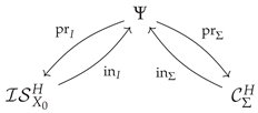
The projected canonical and variation morphisms are

$${\mathrm{can}}_I=\mathrm{can}\circ {\mathrm{in}}_I,{\mathrm{var}}_I={\mathrm{pr}}_I(-1)\circ \mathrm{var}.$$

Their shifted cone triangles are

$$Q_I^H⟶{\mathcal{IS}}_{X_0}^H\stackrel{{\mathrm{can}}_I}{\to }\Phi \stackrel{+1}{\to }$$

and

$$P_I^H⟶\Phi \stackrel{{\mathrm{var}}_I}{\to }{\mathcal{IS}}_{X_0}^H(-1)\stackrel{+1}{\to }.$$

The octahedral comparison of [8] gives

$$P_{\mathrm{var}}^H⟶P_I^H⟶{\mathcal{C}}_{\Sigma }^H(-1)\stackrel{+1}{\to }.$$

In the ordinary-double-point regime of the present paper, ${\mathcal{C}}_{\Sigma }^H=0$, so $P_I^H\simeq P_{\mathrm{var}}^H$ and $Q_I^H\simeq P_{\mathrm{can}}^H$. The projected carriers are retained here because they become genuinely distinct for singularities with nontrivial local monodromy contribution and hence a nonzero Banagl–Budur–Maxim complement.

If the chosen splitting is compatible with Verdier duality, the projected pair satisfies

$$\mathbb{D}{Q}_I^H\simeq P_I^H\left(4\right)\left[1\right],\mathbb{D}{P}_I^H\simeq Q_I^H\left(4\right)\left[1\right].$$

These identities are conditional on the specified duality-compatible splitting and are not used in the ordinary-double-point arguments of the main text.

Finally, the Grothendieck-group comparison between $I{C}_{X_0}^H$ and ${\mathcal{IS}}_{X_0}^H$ does not require an object-level morphism between them. If a mixed-Hodge-module morphism ${\theta }_I:I{C}_{X_0}^H\to {\mathcal{IS}}_{X_0}^H$ is independently supplied, one may form the triangle

$$I{C}_{X_0}^H\stackrel{{\theta }_I}{\to }{\mathcal{IS}}_{X_0}^H⟶C_{I/IC}^H\stackrel{+1}{\to }.$$

The identity ${\Delta }_{I/IC}\left(X_0\right)=[\Phi ]+\left[K\right]$ of Theorem 6 neither requires nor canonically determines such a morphism.

References

- Saito, M. Modules de Hodge polarisables. Publ. Res. Inst. Math. Sci. 1988, 24, 849–995. [Google Scholar] [CrossRef]
- Saito, M. Duality for Vanishing Cycle Functors. Publ. Res. Inst. Math. Sci. 1989, 25, 889–921. [Google Scholar] [CrossRef]
- Saito, M. Mixed Hodge Modules. Publ. Res. Inst. Math. Sci. 1990, 26, 221–333. [Google Scholar] [CrossRef]
- Milnor, J. Singular Points of Complex Hypersurfaces; Vol. 61, Annals of Mathematics Studies; Princeton University Press: Princeton, NJ, 1968. [Google Scholar]
- Dimca, A. Sheaves in Topology; Universitext, Springer-Verlag: Berlin, 2004. [Google Scholar] [CrossRef]
- Banagl, M.; Budur, N.; Maxim, L. Intersection Spaces, Perverse Sheaves and Type IIB String Theory. Adv. Theor. Math. Phys. 2014, arXiv:math18, 363–399. [Google Scholar] [CrossRef]
- Rahman, A. Hodge Atoms at Conifold Degenerations: F-Bundles, Limiting Mixed Hodge Modules, and the Rigid-Flexible Decomposition. arXiv 2026, arXiv:math. [Google Scholar] [CrossRef]
- Rahman, A. Defect Triangles and Intersection-Space Hodge Atom Shadows for Calabi–Yau Conifolds. arXiv 2026, arXiv:math. [Google Scholar] [CrossRef]
- Kerr, M.; Laza, R. Hodge Theory of Degenerations, (II): Vanishing Cohomology and Geometric Applications. In Current Developments in Hodge Theory; Simons Symposia; Springer: Cham, 2025; pp. 299–348. [Google Scholar]
- Schoen, C. Algebraic Cycles on Certain Desingularized Nodal Hypersurfaces. Math. Ann. 1985, 270, 17–27. [Google Scholar] [CrossRef]
- Clemens, H. Homological Equivalence, Modulo Algebraic Equivalence, Is Not Finitely Generated. Publ. Mathématiques De l’IHÉS 1983, 58, 19–38. [Google Scholar] [CrossRef]
- Rossi, M. Geometric Transitions. J. Geom. Phys. 2006, 56, 1940–1983. [Google Scholar] [CrossRef]
- Jung, S.J.; Saito, M. Factoriality of Normal Projective Varieties. arXiv 2026, arXiv:math. [Google Scholar]
- Friedman, G. Generalizations of Intersection Homology and Perverse Sheaves with Duality over the Integers. Mich. Math. J. 2019, 68, 675–726. [Google Scholar] [CrossRef]
- Iritani, H. An Integral Structure in Quantum Cohomology and Mirror Symmetry for Toric Orbifolds. Adv. Math. 2009, arXiv:math222, 1016–1079. [Google Scholar] [CrossRef]
Disclaimer/Publisher’s Note: The statements, opinions and data contained in all publications are solely those of the individual author(s) and contributor(s) and not of MDPI and/or the editor(s). MDPI and/or the editor(s) disclaim responsibility for any injury to people or property resulting from any ideas, methods, instructions or products referred to in the content. |
© 2026 by the author. Licensee MDPI, Basel, Switzerland. This article is an open access article distributed under the terms and conditions of the Creative Commons Attribution (CC BY) license.
Copyright: This open access article is published under a Creative Commons CC BY 4.0 license, which permit the free download, distribution, and reuse, provided that the author and preprint are cited in any reuse.