
Submitted:
31 August 2026
Posted:
31 August 2026
You are already at the latest version
Abstract
We introduce a double golden-ratio Tseng-type extragradient method (DGR--Tseng) for solving variational inequality problems in real Hilbert spaces. The method exploits two golden-ratio averaging steps while requiring only a single projection per iteration. Weak convergence is established under a solution-oriented condition weaker than monotonicity and pseudomonotonicity, without imposing any finiteness assumption on the solution set. Under a Robinson/Luo--Tseng-type local error-bound condition, we further establish \(R\)-linear convergence of the distance to the solution set and a \(Q\)-linear contraction of an associated weighted paired distance, without requiring strong monotonicity, strong pseudomonotonicity, or a singleton solution set. The error bound is weaker than the strong monotonicity-type assumptions commonly used to obtain linear convergence and does not require the solution set to be a singleton. The stepsize is updated adaptively, eliminating the need for prior knowledge of the operator's Lipschitz constant. Numerical experiments on sequence-space and function-space variational inequality problems, together with applications to sparse signal reconstruction and multi-OD urban traffic network equilibrium, demonstrate the computational effectiveness of DGR--Tseng compared with several single golden-ratio methods.
Keywords:
variational inequality
; double golden-ratio method
; adaptive stepsize
; Tseng method
; error bound
; linear convergence
; sparse signal reconstruction
; traffic network equilibrium
MSC: 47H06; 47H09; 47J25; 65K15
1. Introduction
Let C be a nonempty, closed, and convex subset of a real Hilbert space H, and let be an operator. We consider the classical variational inequality problem (VIP) associated with on C, which consists of finding a point such that
The solution set of (1) is denoted by .
The corresponding dual variational inequality problem (DVIP) is to find a point satisfying
The solution set of (2) is denoted by . It is well known that is a closed and convex set, although it may be empty. Moreover, if is continuous and C is convex, then Furthermore, if is continuous and pseudomonotone, then see, for example, Lemma 2.1 in [14]. However, this identity generally fails for continuous quasimonotone operators; see, for instance, Example 4.2 in [53].
Variational inequalities provide a useful framework for problems in economics, engineering mechanics, mathematical programming, transportation science, image reconstruction, signal processing, machine learning, and network equilibrium; see, for example, [1,6,17,24,25,38,55]. This broad range of applications has motivated extensive work on efficient algorithms and their convergence properties. The resulting approaches include projection, extragradient, proximal, splitting, and inertial methods in finite- and infinite-dimensional Hilbert spaces; see, for example, [8,9,10,31,52] and the references therein.
Among the earliest and most fundamental iterative schemes for solving (1) is the gradient projection method, given by
where denotes the metric projection of H onto C and is a stepsize parameter. The convergence of the classical gradient projection method typically requires the operator to be Lipschitz continuous and strongly monotone, or to be inverse strongly monotone.
To weaken these requirements, Korpelevich [26] and independently Antipin [5] introduced the celebrated extragradient method:
where is monotone and L-Lipschitz continuous, and the stepsize satisfies
The extragradient method has inspired many extensions; see, for example, [16,30,43,50] and the references therein. Its main computational drawback is that each iteration requires two metric projections onto C. If projecting onto C is expensive, the second projection can significantly increase the overall cost.
Several methods have therefore been developed to reduce the projection cost, including the subgradient extragradient method [9], Tseng’s forward–backward–forward method [47], and the projection-and-contraction method [21]. These methods reduce the number of projections while retaining desirable convergence properties under suitable assumptions. Even so, most available convergence analyses still rely on monotonicity-type assumptions together with global Lipschitz continuity of the underlying operator.
To enlarge the class of admissible problems, several authors have recently proposed new solution conditions together with extragradient-type methods for non-monotone and non-Lipschitz variational inequalities in real Hilbert spaces; see, for example, [4,46,49]. Moreover, a number of existing convergence analyses impose the additional requirement that the set be finite; see, for instance, Condition (A5’) in [27]. This requirement is restrictive because it excludes variational inequality problems for which may contain infinitely many points. Here we avoid the finiteness assumption by using the solution-oriented condition (A2), which relates on the feasible set only to points in the solution set. This condition is implied by monotonicity and pseudomonotonicity, but is less restrictive than either of these assumptions [46].
In a parallel direction aimed at reducing the projection cost per iteration, Malitsky [32] introduced an elegant iterative framework based on the golden ratio for solving the mixed variational inequality problem of finding such that
where is a monotone operator and is a proper, convex, and lower semicontinuous function. To solve (5), he proposed the following golden-ratio algorithm:
where
is the golden ratio, and denotes the proximal operator associated with g.
When , the indicator function of a nonempty closed and convex set C, problem (5) reduces to the classical variational inequality problem (1), while the proximal mapping becomes the metric projection:
A useful feature of the golden-ratio algorithm is that the auxiliary iterate is generated through a golden-ratio convex combination of previously computed points. The method therefore uses information from earlier iterates while requiring only one proximal or projection evaluation per step. Since its introduction, golden-ratio techniques have inspired numerous extensions for variational inequalities, equilibrium problems, fixed-point problems, and monotone inclusions; see, for example, [2,3,11,12,13,23,39,40,54] and the references therein.
Most existing golden-ratio methods use a single extrapolation step. To the best of our knowledge, no double golden-ratio Tseng-type extragradient method has yet been developed. This leads us to ask whether two golden-ratio averaging mechanisms can make better use of previous iterates while preserving a low per-iteration cost.
Linear convergence is important both theoretically and computationally. Existing R-linear convergence results for variational inequality algorithms are mainly established under relatively strong assumptions such as strong monotonicity or strong pseudomonotonicity, typically together with global Lipschitz continuity of the underlying operator; see, for example, [2,3,13,20,34,40,45,54]. Although these assumptions yield linear convergence, they restrict the range of admissible problems and force the solution set to be a single point. Below we obtain R-linear convergence of and a Q-linear contraction of an associated weighted paired distance under a local error-bound condition of Robinson/Luo–Tseng type, without imposing strong monotonicity or requiring to be a singleton.
Motivated by these observations, we develop a double golden-ratio Tseng-type extragradient method for variational inequalities in real Hilbert spaces. Its two averaging steps retain information from previous iterates without adding another projection. The analysis uses a solution-oriented condition in place of the usual monotonicity assumptions. The method also updates its stepsize adaptively; unlike (4), where must be chosen in advance, it can be implemented without knowing the Lipschitz constant.
The main contributions of this paper are summarized as follows.
- (i)
- We introduce a double golden-ratio Tseng-type extragradient algorithm that uses two averaging steps to retain information from previous iterates while requiring only one projection per iteration.
- (ii)
- (iii)
- An adaptive stepsize removes the need to know the Lipschitz constant of in advance. The operator is still assumed globally Lipschitz continuous, but this constant never has to be computed or estimated to run the algorithm.
- (iv)
- Unlike the R-linear results in [2,3,13,20,34,40,45,54], we prove weak convergence of to a point of , and R-linear convergence of to 0, under a Robinson/Luo–Tseng-type local error bound without assuming strong monotonicity or strong pseudomonotonicity and without forcing to be a singleton. The error bound is weaker than the strong monotonicity-type assumptions commonly used to obtain linear convergence and does not require the solution set to be a singleton.
- (v)
- Under the same error bound, we obtain a Q-linear contraction of a weighted paired distance for all sufficiently large iterations. When is a singleton, the weighted paired error remains Q-linear, while the iterates satisfy an explicit R-linear estimate.
- (vi)
- Numerical experiments on sequence-space and function-space variational inequality problems, together with applications to sparse signal reconstruction and multi-OD urban traffic network equilibrium, demonstrate the computational effectiveness of DGR–Tseng. In comparison with several well-known single golden-ratio methods, the proposed method exhibits favorable performance in terms of iteration counts, CPU time, and solution accuracy, as well as reconstruction and traffic-equilibrium performance measures in the respective applications.
The rest of the paper is organized as follows. Section 2 collects the preliminary facts, identities, and lemmas used throughout. Section 3 presents the proposed algorithm, while Section 4 establishes its weak convergence. Section 5 develops R-linear convergence under a local error-bound condition, and Section 6 sharpens this to Q-linear convergence. Section 7 reports numerical experiments, Section 8 presents an application to sparse signal reconstruction, and Section 9 applies the method to a multi-OD urban traffic network equilibrium problem. Finally, Section 10 concludes the paper.
2. Preliminaries
Throughout, is a real Hilbert space with inner product and induced norm , and is a nonempty closed convex subset of . We write for weak convergence and for strong convergence of a sequence . Recall the identity
and that for every there is a unique nearest point ; the operator is nonexpansive.
Lemma 1.
For every and every ,
Lemma 2
Moreover, for every and ,
We omit the proof, which is standard.
Lemma 3
([35]). Let and let be nonempty. If
- (a)
- exists for every , and
- (b)
- every weak sequential cluster point of lies in Ω,
then converges weakly to a point of Ω.
Lemma 4
([44]). Let , be nonnegative real sequences with for all k and . Then exists.
Lemma 5
In particular, if is nonempty, closed and convex, the distance function is convex (indeed 1-Lipschitz), so for every and ,
Lemma 6
(Perron–Frobenius theorem, [22] (Theorem 8.4.4)). Let have nonnegative entries and be irreducible. Then there is a real number , the Perron root of N, such that:
- (i)
- for every eigenvalue ξ of N (i.e. equals the spectral radius of N);
- (ii)
- is a simple eigenvalue of N;
- (iii)
- N has an eigenvector associated with all of whose entries are strictly positive.
Lemma 7
(Gelfand’s spectral radius formula, [18,22] (Corollary 5.6.14)). Let and let be any submultiplicative matrix norm. Then
Consequently, for every there exists a constant , depending only on N, σ and the chosen norm, such that
Definition 1
(Robinson/Luo–Tseng-type error bound, [28,29,41]). Let be nonempty, closed and convex, let , and let . The pair is said to admit aRobinson/Luo–Tseng-type local error boundat Ω if there exist , and a compact interval such that
for every and every satisfying . The bound is calledglobalwhen . Robinson’s polyhedral error-bound theorem [41] shows that a global bound of this type holds whenever is polyhedral and is affine; Luo and Tseng [28,29] extended this to piecewise-affine and, more generally, essentially smooth on polyhedral , and to the associated variational-inequality residuals used above.
3. Proposed Method
We work under the following assumptions.
Assumption 1.
- (A1)
- is L-Lipschitz continuous for some :
- (A2)
- for every and ;
- (A3)
- implies for every ;
- (A4)
- is nonempty, closed and convex.
The proposed method is given below.
| Algorithm 1 Adaptive Double Golden-Ratio Tseng Method (DGR-Tseng) |
|
Initialization: Choose , , , , , , such that , , . Set .
Iterative steps: Given the current iterates , , and , calculate as follows:
Step 1. Compute
Step 2. Compute
If , then stop. Otherwise, go to Step 3.
Step 3. Compute
Step 4. Set
Step 5. Update
Set and return to Step 1.
|
Remark 1.
We fix throughout the constants attached to , :
Remark 2.
- If , then , and Lemma 2 gives for all , so and the stopping rule is well defined.
- Condition (A2) is less restrictive than monotonicity or pseudomonotonicity, since it only relates points of to points of the solution set.
- When , the two averaging steps use the same classical golden-ratio weighting, , and . Accordingly, the Lyapunov function of Lemma 10 becomes .
4. Weak Convergence Analysis
We begin with the behaviour of the step-size sequence, which under the global Lipschitz assumption (A1) can be bounded away from zero. The update rule (14) does not multiply the ratio by the bare constant , but by the k-dependent factor , so it is this factor, not alone, that has to be tracked. To keep the notation light we write Because and , we always have ; and because , , we also have . Both facts are used repeatedly below.
Lemma 8.
Let be generated by (14) and set and . Then for every k, and converges to some . Furthermore
Proof.
We induct on the floor bound. At it holds because . Assume . If , the second branch of (14) gives outright. If instead , then , and (A1) bounds the numerator: , so
the last step using noted above. Since (14) takes the minimum of this quantity with , we get , as by the choice of m. This closes the induction, and in particular the correction term and the slack factor never push the stepsize below the same floor m that a fixed constant would have given.
For the upper bound, (14) gives in either branch. Hence . Therefore . Since , Lemma 4 yields the convergence of to some .
Finally, (15) is immediate when , and otherwise follows directly from the definition by rearranging. □
Remark 3.
The global Lipschitz condition (A1) is essential for this lower bound. Under the weaker uniform continuity assumption used in [4,46], one can only show that , leaving open the possibility that the step size decays to zero. That possibility must then be addressed separately in the convergence proof. Here, the explicit bound rules it out.
Lemma 9.
Suppose (A2) holds. For every and ,
Proof.
Since and , Lemma 2 gives
By (12), we have
Inserting (17) and noting that , we get
By (A2), because and , so the corresponding term may be discarded:
It is at this point that the correction terms in the stepsize rule matter, and it is also here that they stop mattering: by Lemma 8, , so ; and by construction. Hence , and since ,
Lemma 10.
Suppose (A2) holds and let c be as in Remark 1. For and set . Then there are constants , not depending on k or u, such that
Consequently converges for every ,
the sequences , , , are bounded, and exists for every .
Proof.
The two bracketed coefficients simplify considerably once we recall that c was chosen so that . Indeed
and
where the last step uses once more. So the coefficients of collapse to exactly, and we arrive at (21) with , , , all strictly positive by Remark 1.
Because , the sequence is nonincreasing and nonnegative, hence convergent, and telescoping (21) from to ∞ gives
which yields (22).
Boundedness of follows from for , and boundedness of from (10), since is a convex combination of and . Boundedness of and is then immediate from (22).
For the last claim, note bounded gives some with , and hence
Writing , convergence of together with forces to converge as well. □
Lemma 11.
Suppose (A1)–(A4) hold, and let be a subsequence of with and . Then .
Proof.
From and we get , and since with weakly closed, .
Let be arbitrary. Since , Lemma 2 gives
i.e. . Dividing by and splitting inside the left-hand inner product gives
The sequence is bounded, so by (A1) so is ; combined with this gives a bounded and . By Lemma 8, for every j, so is bounded, and Cauchy–Schwarz applied to both terms on the left of (24) shows that each vanishes as :
Hence
Applying (A3) to , , , and using (25),
As was arbitrary, . □
Theorem 1.
Under Assumption 1, if , and , the sequence generated by Algorithm 1 converges weakly to a point of Ω.
Proof.
Condition (a) of Lemma 3 is exactly what Lemma 10 gives us: exists for every .
For condition (b), take any weakly convergent subsequence . We would like to place in via Lemma 11, but that lemma speaks about , not – so we first move the subsequence over. Since by (22), inherits the same weak limit ; and since as well, the residual too. Both hypotheses of Lemma 11 are met by the subsequence indexed by , so .
With both conditions of Lemma 3 in hand, converges weakly to a point of . □
5. R-Linear Convergence
By Lemma 8, every stepsize generated by the algorithm satisfies , where and . We impose a local Robinson/Luo–Tseng-type error bound uniformly over this fixed interval.
Assumption A2.
There exist and such that, for every and every satisfying ,
Example 1.
Let , , and define by
Since , we have , and the variational inequality is equivalent to . Hence, which is not a singleton. For every , Moreover, for every ,
and therefore
Thus, for every ,
so Assumption 2 holds globally with . On the other hand, is not strongly monotone. Indeed, for and ,
Hence no can satisfy
for all . Therefore, the error-bound condition may hold even when strong monotonicity fails and the solution set is not a singleton.
Remark 4.
Example 1 shows that Assumption 2 may hold even when strong monotonicity fails and the solution set is not a singleton. Thus the linear-rate analysis below is based on an error-bound property rather than on the strong monotonicity-type assumptions commonly used to obtain linear convergence.
Recall , and that is convex and 1-Lipschitz because is closed and convex (Lemma 5).
Lemma 12.
Suppose (A2) and Assumption 2 hold. Let
and let be as in (19) for this choice of θ. Then there exists such that, for every ,
where .
Proof.
For and , write . Since , the nonexpansiveness of and (A1) give
By (22), . Hence there exists such that for every . Because and , Assumption 2 yields
Therefore
Write , so . Since , inequality (20) gives, for ,
Since and , the number belongs to . Finally, , which proves (27). □
Lemma 13.
Set , , and . Then, for all ,
with as in Remark 1 and γ as in Lemma 12.
Proof.
Since is closed and convex, is convex, so Jensen’s inequality (Lemma 5, specifically (8)) applied to gives
Applying Jensen’s inequality (Lemma 5) to and then Lemma 12,
Since , inserting (29) preserves the inequality:
Lemma 14.
The matrix N of Lemma 13 has nonnegative, irreducible entries, and .
Proof.
Nonnegativity is clear since and ; irreducibility holds because both off-diagonal entries and are strictly positive. A direct computation gives
where T is strictly increasing in . By the Perron–Frobenius theorem (Lemma 6), N has a real, positive, simple dominant eigenvalue at least as large in modulus as any other eigenvalue; for a real matrix the remaining eigenvalue is then automatically real, so are the two roots of and, by part (i) of Lemma 6,
which is strictly increasing in T (its T-derivative is ). At , one checks directly (as in the coefficient identity of Lemma 10) that solves , so and . Since implies , monotonicity gives . □
Theorem 2.
Suppose (A1)–(A4) and Assumption 2 hold, and let be generated by Algorithm 1 with , and . Then there exist and such that
That is, converges to Ω R-linearly. Consequently, together with Theorem 1, converges weakly to some with at the geometric rate (30); if in addition is a singleton, this reads , i.e. strong convergence at a linear rate.
Proof.
Since N has nonnegative entries, entrywise inequalities propagate under repeated multiplication: from Lemma 13, entrywise for every . By Lemma 14, , so by Gelfand’s spectral radius formula (Lemma 7), for any there is with for all (in any fixed matrix norm). The vector is finite and nonnegative, since and are bounded by Lemma 10 (which uses only (A2)). Hence each entry of is bounded by for a suitable constant ; in particular for all . Writing gives (30). □
Remark 5.
Assumption 2 is imposed only on points of . Lemma 12 applies it at and then transfers the resulting estimate to by nonexpansiveness of the projection and Lipschitz continuity of . Thus the error bound is never applied to an iterate outside its stated domain. Moreover, Lemma 13 uses Jensen’s inequality (Lemma 5) for the convex function , so the matrix recursion propagates distances rather than squared distances.
6. Q-Linear Convergence
Theorem 2 of Section 5 is an R-linear statement: it only bounds by a fixed geometric envelope, for some strictly larger than , via Gelfand’s formula (Lemma 7), which is inherently asymptotic. We now show that the same matrix inequality (28) in fact yields a genuine, non-asymptotic Q-linear contraction with the explicit Perron factor once and are combined through the left Perron eigenvector of N. Throughout this section we retain Assumption 2 and all the notation of Section 5 (, etc.).
Lemma 15.
Let N be the matrix of Lemma 13. The transpose is again nonnegative and irreducible, since transposition preserves both properties. Hence Lemma 6, applied to , yields together with an eigenvector of associated with all of whose entries are strictly positive, i.e.
Theorem 3.
Suppose (A1)–(A4) and Assumption 2 hold, let be generated by Algorithm 1 as in Theorem 2, and let be the left Perron eigenvector of Lemma 15. Define, for ,
Then
that is, converges Q-linearly to 0 with ratio . Consequently
which provides an explicit R-linear estimate for with geometric factor and constant , instead of an arbitrary and the Gelfand constant .
Proof.
Fix . By Lemma 13, entrywise, where . Since , left-multiplying an entrywise inequality between nonnegative vectors by preserves it:
Remark 6.
Neither Theorem 2 nor Theorem 3 assumes strong monotonicity or strong pseudomonotonicity of . Theorem 2 gives R-linear convergence of , whereas Theorem 3 gives Q-linear convergence of the weighted paired distance . Assumption 2 does not force Ω to be a singleton, so both conclusions remain meaningful for a non-singleton solution set.
7. Numerical Examples
This section illustrates the convergence results established in Section 5Section 6 and examines the numerical performance of the proposed Adaptive Double Golden-Ratio Tseng method (DGR-Tseng), given in Algorithm 1. We compare DGR-Tseng with three golden-ratio-type methods from the literature, namely:
Unlike DGR-Tseng, which uses the double golden-ratio mechanism (10)–(13), the competing methods employ a single golden-ratio extrapolation step.
All computations were carried out in MATLAB R2018a. In Example 2, the space was approximated by its first coordinates. In Example 3, the interval was discretized using 501 equally spaced grid points, and the -norm and the required integrals were approximated by the composite trapezoidal rule.
For each test case, the same initial data were used for all four algorithms. The common stopping criterion was , with a maximum of 1500 iterations.
Let The control parameters used in the experiments are listed in Table 1.
The selected sequences satisfy for DGR-Tseng, and for GRT-Tseng and SEM-GRT.
We consider two infinite-dimensional test problems. The first is posed in , while the second is formulated in . In both examples, the operator is globally Lipschitz continuous but nonmonotone, and the solution set is .
Example 2.
Let and define Consider Set
We first note that
If , then , so If , then and again Since we have
Thus is 3-Lipschitz continuous.
Because , the variational inequality reduces to . From (35), and hence Therefore, Furthermore,
Hence Assumption(A2)holds.
Let in . Since , and with we have . For ,
Using the weak lower semicontinuity of the norm gives
Thus Assumption(A3)holds, while Assumption(A4)follows from .
The operator is nonmonotone since Thus there exist such that Setting gives
Finally, Since , for every ,
Hence Assumption 2 holds globally with
For the numerical test, was truncated to its first coordinates. For , we used
Case 3:(p0)j=3.5(0.35j)j, (p1)j=2.5(0.25j)j, (w0)j=1.5(0.50j)j,
Case 4:(p0)j= 3(0.20j)+(0.60j)j,
(p1)j= 2.5(0.30j)-0.8(0.70j)j, (w0)j= 1.5(0.40j)+0.5(0.90j)j.
Example 3.
Let e(t)=1. Then . Define
Every can be written uniquely as Let and define
For and ,
Hence is 3-Lipschitz continuous.
Since , the variational inequality reduces to . Using we obtain
Moreover,
so Assumption(A2)holds.
If , write Then and . For , ,
Weak lower semicontinuity yields the required limit inequality, so Assumption(A3)follows. Assumption (A4)follows from .
The operator is nonmonotone. Indeed, for sufficiently small , take Since , Furthermore, and therefore
Hence Assumption 2 holds globally with
For the numerical experiment, four starting-point cases were used:
8. Application to Sparse Signal Reconstruction
We next consider an application to sparse signal reconstruction. Let denote the unknown sparse signal and suppose that
where , , is the sensing matrix and represents measurement noise.
We consider the regularized problem
where is nonempty, closed, and convex, and . Its gradient is given by Define The corresponding first-order condition can be written as
The gradient of the least-squares term, , is Lipschitz continuous with constant . Moreover, is globally Lipschitz continuous because the derivative of each scalar component is bounded in modulus by . Hence is globally Lipschitz continuous with Lipschitz constant at most . Since is nonconvex, the resulting operator need not be monotone.
We consider , and The sensing matrix is generated according to and additive Gaussian noise is included in the measurements. For visual comparison, the back-projected signal is also displayed.
The reconstruction quality is measured using
and
Thus, smaller MSE and larger SNR indicate better reconstruction.
For each dimension, Figure 7, Figure 8, Figure 9 and Figure 10 show the original signal, the back-projected noisy measurement, and the reconstructions produced by the four methods.
Table 4 shows that DGR-Tseng gives the lowest MSE and the highest SNR in all four cases. For , DGR-Tseng attains an MSE of and an SNR of dB, while GRT-Tseng, the next-best method in this case, records and dB.
The same pattern persists as the dimension increases. For , DGR-Tseng achieves an MSE of and an SNR of dB, compared with SNR values of , , and dB for GRT-Tseng, SEM-GRT, and GRPA, respectively. Together with the reconstruction plots, these results show that DGR-Tseng more closely reproduces the significant coefficients of the original sparse signal in the reported experiment.
9. Application to a Multi-OD Urban Traffic Network Equilibrium Problem
Traffic network equilibrium is one of the classical applications of variational inequality theory. According to Wardrop’s user-equilibrium principle [51], a traffic flow is at equilibrium if no traveller can reduce the experienced travel cost by unilaterally switching to another admissible route connecting the same origin and destination. The classical optimization formulation of traffic assignment was developed by Beckmann et al. [7], while its more general variational inequality formulation was studied by Dafermos [15]; see also [33,37].
In this section, we apply the proposed DGR–Tseng method to a multi-origin–destination urban traffic network involving nonlinear congestion, asymmetric route interaction, and incident-induced capacity reductions. Besides providing a practical illustration of the variational inequality framework, the example permits a route-level and network-level comparison of DGR–Tseng with GRPA, GRT–Tseng, and SEM–GRT.
Let be the directed traffic network with node set The nodes W and S are the two origins, while is the common destination. We consider the two origin–destination pairs with traffic demands
The complete network consists of fourteen directed links and is displayed in Figure 13.
The free-flow travel times and nominal capacities are given in Table 5.
For the OD pair , the admissible routes are
while for we consider
These routes are displayed in Figure 14.
Let denote the path-flow vector, where is the flow assigned to route . The feasible path-flow set is
Thus where and are simplices. In particular, is nonempty, closed, bounded, convex, and polyhedral.
Let be the link–path incidence matrix defined by
For the eight routes under consideration,
Hence, the link-flow vector corresponding to p is
For every link , its travel time is modelled by the BPR-type volume-delay function [48]
To represent an incident-sensitive bottleneck, the effective capacity of is reduced to whereas the effective capacity of the merging link is reduced to For all other links, The route-cost component generated by the link travel times is
To incorporate interaction among different traffic streams, define the operator by
where has the nonzero entries
The asymmetric term provides a simplified representation of cross-route interaction, merging interference, and spillback.
The traffic equilibrium problem is therefore to find such that
Thus, (46) is precisely a finite-dimensional instance of the variational inequality problem studied throughout this paper, with solution set Since , its metric projection satisfies Consequently, the single projection required at each DGR–Tseng iteration reduces to two standard simplex projections.
Since is compact and the BPR travel-time functions are continuously differentiable on the relevant bounded traffic range, is Lipschitz continuous on . However, the quartic BPR extension is not globally Lipschitz continuous on all of , and the iterates need not remain in . Accordingly, this section is intended as a computational application of the proposed method; we do not claim that this particular traffic model satisfies the global Lipschitz assumption (A1) or the error-bound hypothesis of Section 5Section 6 on the whole ambient space.
Algorithm 1 generates the sequence together with , , and . Since , whereas need not necessarily belong to , we use the feasible diagnostic path-flow vector when reporting traffic-specific quantities. The normalized natural residual is defined by Accordingly, the residual reported at iteration k is .
For each OD pair, define The associated Wardrop relative gaps are
and
We set
The two network-level traffic indicators are and Thus, the reported performance quantities are
The common tolerance is and the traffic stopping test is To examine sensitivity to initialization, we define the four feasible base path-flow vectors
For each case , Algorithm 1 is initialized by This choice is admissible under the initialization of Algorithm 1 and provides a uniform starting state for the main and auxiliary sequences. Moreover, since For fairness, the same base path-flow vector is used to initialize each competing method in Case j, according to its respective initialization rule.
For the experiment in this section, we maintain the same control parameters as in Section 7. The high-accuracy reference equilibrium is computed using tolerance and a maximum of 20000 iterations.
For a fair numerical comparison, DGR–Tseng, GRPA, GRT–Tseng, and SEM–GRT are considered on the same traffic equilibrium problem using the same starting-point cases and stopping criterion. The reported iteration counts, CPU times, terminal natural residuals, Wardrop relative gaps, total system travel times (TSTT), and maximum volume-to-capacity ratios (MaxVC) are used to compare the methods in terms of computational efficiency, equilibrium accuracy, and the quality of the resulting network traffic states.
The numerical results for the four initial path-flow cases are reported in Table 6.
The results in Table 6 show that DGR–Tseng attains the smallest iteration count, CPU time, natural residual, and Wardrop relative gap in all four cases. In addition, the traffic states obtained by DGR–Tseng yield the smallest TSTT and MaxVC values among the four methods.
Figure 15 displays the natural residual and Wardrop relative gap for Case 1.
Both quantities are displayed on logarithmic scales. The trajectories exhibit method-dependent curvature, transient behaviour, changes of slope, and different termination points. In particular, the DGR–Tseng profile reaches the terminal accuracy in substantially fewer iterations.
Figure 16 compares the iteration counts and CPU times for the four initial path-flow cases.
Figure 17 shows the corresponding terminal accuracy.
Since increases as decreases, a taller bar represents a smaller error. Thus, DGR–Tseng attains the highest terminal accuracy in all four cases.
Let denote the high-accuracy reference equilibrium computed by DGR–Tseng. To supplement the direct solver comparison with a route-level sensitivity analysis around this reference equilibrium, define
where is a demand-preserving perturbation direction and The four components are associated, respectively, with DGR–Tseng, GRPA, GRT–Tseng, and SEM–GRT. These reference-based states are used only for the supplementary route- and link-level sensitivity comparisons below; the direct algorithmic results are those reported in Table 6.
The associated generalized route-cost vectors are
Figure 18 compares the resulting route flows and generalized route costs.
Neither a smaller nor a larger individual route flow is intrinsically better, since the route flows jointly satisfy the fixed OD demands. For this supplementary sensitivity comparison, the relevant quantity is proximity to the reference equilibrium. In particular, the selected reference-based states satisfy
for each competing method m, together with the analogous route-cost comparison.
The corresponding link-flow vectors are and their link volume-to-capacity ratios are
Figure 19 displays the corresponding network-loading patterns.
The threshold corresponds to effective link capacity; values exceeding one therefore indicate overloaded links. As in the route-flow comparison, the magnitude of an individual link flow is not itself an algorithmic accuracy measure. Rather, proximity to the reference loading and the resulting level of congestion provide the appropriate interpretation.
The aggregate traffic-state indicators are reported in Figure 20.
For the computed traffic states, a smaller TSTT represents a smaller aggregate network travel time, whereas a smaller MaxVC indicates a less severe peak congestion level. These are descriptive network indicators rather than variational-inequality residuals, and TSTT is not a system-optimality certificate for a Wardrop equilibrium. The DGR–Tseng traffic state gives the smallest values of both quantities in each of the four cases.
Remark 7.
The traffic experiment provides complementary algorithmic and transportation-level information. Figure 13 and Figure 14 describe the network structure and the eight admissible routes. Figure 15 illustrates the natural-residual and Wardrop-gap trajectories, while Figure 16 and Figure 17 compare the computational effort and terminal accuracy across the four initial path-flow cases.
At the transportation level, Figure 18 compares route flows and generalized route costs with the high-accuracy reference equilibrium, whereas Figure 19 shows the induced link loading and congestion. Figure 20 summarizes the corresponding total system travel time and maximum volume-to-capacity ratio.
The numerical results show that DGR–Tseng exhibits the most favorable iteration count, CPU time, natural residual, and Wardrop relative gap in all four cases. The supplementary reference-based route and link states associated with DGR–Tseng are closest to the high-accuracy reference equilibrium, and the corresponding traffic states have the smallest TSTT and MaxVC values.
The experiment therefore illustrates the potential usefulness of the double golden-ratio mechanism for a structured multi-OD traffic equilibrium problem involving nonlinear congestion, asymmetric route interaction, and incident-sensitive capacities.
10. Conclusions
In this paper, we introduced an adaptive double golden-ratio Tseng-type extragradient method, called DGR–Tseng, for solving variational inequality problems in real Hilbert spaces. The method employs two golden-ratio averaging steps while requiring only one metric projection per iteration. Its adaptive stepsize also removes the need for prior knowledge of the Lipschitz constant.
Under the solution-oriented assumptions adopted in this work, we established weak convergence of the generated sequence to a point of . Under an additional Robinson/Luo–Tseng-type local error-bound condition, we proved R-linear convergence of and a Q-linear contraction for the associated weighted paired distance. These linear convergence results do not require strong monotonicity, strong pseudomonotonicity, or a singleton solution set.
The theoretical results were supported by numerical experiments in and , together with applications to sparse signal reconstruction and multi-OD urban traffic network equilibrium. The reported results show that DGR–Tseng compares favorably with GRPA, GRT–Tseng, and SEM–GRT in terms of iteration counts, CPU time, and convergence accuracy. It also produced favorable reconstruction and traffic-equilibrium performance measures in the respective applications.
These results demonstrate the effectiveness of the double golden-ratio mechanism for projection-efficient variational inequality methods beyond the standard monotonicity setting. Future work may consider extensions to non-Lipschitz operators, split and bilevel variational inequalities, and related equilibrium and inclusion problems.
Institutional Review Board Statement
Not applicable.
Data Availability Statement
The numerical data used in this study are generated computationally as described in the manuscript and are available from the corresponding author upon reasonable request.
Conflicts of Interest
The authors declare no conflict of interest.
References
- R. Abaidoo and E. K. Agyapong, Financial development and institutional quality among emerging economies, J. Econ. Dev., 24 (2022), 198–216. [CrossRef]
- H. A. Abass, A. E. Ofem and M. Aphane, Efficient step size rule and golden ratio technique for solving quasimonotone variational inequalities, Carpathian J. Math., 42 (2026), 755–772. [CrossRef]
- K. S. Abiodun, O. K. Narain, A. E. Ofem and O. K. Oyewole, A Tseng algorithm based on the golden ratio technique for solving variational inequality problems in Hilbert spaces, J. Anal., 34 (2026), 1423–1444. [CrossRef]
- A. Adamu, D. V. Thong, N. T. An and D. H. Ngan, Solving non-monotone variational inequality problems involving non-Lipschitz mappings with application to image restoration, J. Sci. Comput., 107 (2026), 75. [CrossRef]
- A. S. Antipin, On a method for convex programs using a symmetrical modification of the Lagrange function, Ekon. Mat. Metody, 12 (1976), 1164–1173.
- C. Baiocchi and A. Capelo, Variational and Quasivariational Inequalities: Applications to Free Boundary Problems, Wiley, New York, 1984.
- M. J. Beckmann, C. B. McGuire and C. B. Winsten, Studies in the Economics of Transportation, Yale University Press, New Haven, 1956.
- Y. Censor, A. Gibali and S. Reich, Strong convergence of subgradient extragradient methods for the variational inequality problem in Hilbert space, Optim. Methods Softw., 26 (2011), 827–845. [CrossRef]
- Y. Censor, A. Gibali and S. Reich, The subgradient extragradient method for solving variational inequalities in Hilbert space, J. Optim. Theory Appl., 148 (2011), 318–335. [CrossRef]
- Y. Censor, A. Gibali and S. Reich, Extensions of Korpelevich’s extragradient method for the variational inequality problem in Euclidean space, Optimization, 61 (2012), 1119–1132. [CrossRef]
- X. Chang and J. F. Yang, A golden ratio primal-dual algorithm for structured convex optimization, J. Sci. Comput., 87(2) (2021), 1–26. [CrossRef]
- X. Chang, J. F. Yang and H. C. Zhang, Golden ratio primal-dual algorithm with linesearch, SIAM J. Optim., 32(3) (2022), 1584–1613. [CrossRef]
- Z. Chu and C. Zhang, R-linear convergence analysis of two golden ratio projection algorithms for strongly pseudo-monotone variational inequalities, Optimization Eruditorum, 1(1) (2024), 45–55. [CrossRef]
- R. W. Cottle and J. C. Yao, Pseudo-monotone complementarity problems in Hilbert space, J. Optim. Theory Appl., 75 (1992), 281–295. [CrossRef]
- S. Dafermos, Traffic equilibrium and variational inequalities, Transp. Sci., 14 (1980), 42–54. [CrossRef]
- S. V. Denisov, V. V. Semenov and L. M. Chabak, Convergence of the modified extragradient method for variational inequalities with non-Lipschitz operators, Cybern. Syst. Anal., 51 (2015), 757–765. [CrossRef]
- F. Facchinei and J. S. Pang, Finite-Dimensional Variational Inequalities and Complementarity Problems, Volume I, Springer Series in Operations Research, Springer, New York, 2003.
- I. Gelfand, Normierte Ringe, Rec. Math. [Mat. Sbornik] N.S., 9(51) (1941), 3–24.
- K. Goebel and S. Reich, Uniform Convexity, Hyperbolic Geometry, and Nonexpansive Mappings, Marcel Dekker, New York, 1984.
- L. T. T. Hai, D. V. Thong and P. T. Vuong, An inertial extragradient method for solving strongly pseudomonotone equilibrium problems in Hilbert spaces, Comput. Appl. Math., 43 (2024), 363. [CrossRef]
- B. S. He, A class of projection and contraction methods for monotone variational inequalities, Appl. Math. Optim., 35 (1997), 69–76. [CrossRef]
- R. A. Horn and C. R. Johnson, Matrix Analysis, 2nd ed., Cambridge University Press, Cambridge, 2013.
- C. Izuchukwu and Y. Shehu, A golden ratio algorithm with backward inertial step for variational inequalities, Commun. Nonlinear Sci. Numer. Simulat., 138 (2024), 108217. [CrossRef]
- D. Kinderlehrer and G. Stampacchia, An Introduction to Variational Inequalities and Their Applications, Academic Press, New York, 1980.
- I. V. Konnov, Combined Relaxation Methods for Variational Inequalities, Springer-Verlag, Berlin, 2001.
- G. M. Korpelevich, The extragradient method for finding saddle points and other problems, Ekon. Mat. Metody, 12 (1976), 747–756.
- H. Liu and L. Yang, Weak convergence of iterative methods for solving quasimonotone variational inequalities, Comput. Optim. Appl., 77 (2020), 491–508. [CrossRef]
- Z.-Q. Luo and P. Tseng, On the linear convergence of descent methods for convex essentially smooth minimization, SIAM J. Control Optim., 30(2) (1992), 408–425. [CrossRef]
- Z.-Q. Luo and P. Tseng, Error bounds and convergence analysis of feasible descent methods: a general approach, Ann. Oper. Res., 46(1) (1993), 157–178. [CrossRef]
- P. E. Maingé, A hybrid extragradient-viscosity method for monotone operators and fixed point problems, SIAM J. Control Optim., 47 (2008), 1499–1515. [CrossRef]
- Y. V. Malitsky, Projected reflected gradient methods for monotone variational inequalities, SIAM J. Optim., 25 (2015), 502–520. [CrossRef]
- Y. Malitsky, Golden ratio algorithms for variational inequalities, Math. Program., 184(1) (2020), 383–410. [CrossRef]
- A. Nagurney, Network Economics: A Variational Inequality Approach, 2nd ed., Kluwer Academic Publishers, Boston, 1999.
- F. O. Nwawuru, J. N. Ezeora, H. Rehman and J.-C. Yao, Two parallel golden ratio iterative algorithms for approximate solution of equilibrium problem in real Hilbert space, Commun. Nonlinear Sci. Numer. Simulat. (2026), 110622. [CrossRef]
- Z. Opial, Weak convergence of the sequence of successive approximations for nonexpansive mappings, Bull. Amer. Math. Soc., 73 (1967), 591–597. [CrossRef]
- O. K. Oyewole and S. Reich, Two subgradient extragradient methods based on the golden ratio technique for solving variational inequality problems, Numer. Algorithms, 97 (2024), 1215–1236. [CrossRef]
- M. Patriksson, The Traffic Assignment Problem: Models and Methods, Topics in Transportation, VSP, Utrecht, 1994.
- J.-W. Peng, J.-J. Luo and A. Adamu, A two-step inertial method with a new step-size rule for quasimonotone variational inequalities in Hilbert spaces, Optimization Eruditorum, 2 (2025), 184–199.
- J. W. Peng, L. Han, A. Adamu and J. C. Yao, Strongly convergent golden ratio algorithm for pseudomonotone variational inequalities with applications, Numer. Algorithms (2026). [CrossRef]
- H. Rehman, Z.-Y. Peng and J.-C. Yao, Approximate subgradient extragradient methods for solving variational inequality problems: convergence analysis and applications in signal and image processing, Commun. Nonlinear Sci. Numer. Simulat., 152 (2026), 109211. [CrossRef]
- S. M. Robinson, Some continuity properties of polyhedral multifunctions, Math. Programming Stud., 14 (1981), 206–214. [CrossRef]
- R. T. Rockafellar, Convex Analysis, Princeton University Press, Princeton, NJ, 1970.
- M. V. Solodov and B. F. Svaiter, A new projection method for variational inequality problems, SIAM J. Control Optim., 37 (1999), 765–776. [CrossRef]
- K. K. Tan and H. K. Xu, Approximating fixed points of nonexpansive mappings by the Ishikawa iteration process, J. Math. Anal. Appl., 178 (1993), 301–308. [CrossRef]
- D. V. Thong and P. T. Vuong, R-linear convergence analysis of inertial extragradient algorithms for strongly pseudo-monotone variational inequalities, J. Comput. Appl. Math., 406 (2022), 114003. [CrossRef]
- D. V. Thong, Convergence analysis of a self-adaptive inertial subgradient extragradient method for non-monotone variational inequalities with non-Lipschitz continuous mappings, Numer. Algorithms (2026). [CrossRef]
- P. Tseng, A modified forward-backward splitting method for maximal monotone mappings, SIAM J. Control Optim., 38 (2000), 431–446. [CrossRef]
- U.S. Bureau of Public Roads, Traffic Assignment Manual for Application with a Large, High-Speed Computer, U.S. Department of Commerce, Bureau of Public Roads, Office of Planning, Urban Planning Division, Washington, DC, 1964.
- T. D. Viet, A new method for solving non-monotone variational inequalities based on extragradient method, J. Ind. Manag. Optim., 21 (2025), 6913–6927. [CrossRef]
- P. T. Vuong, On the weak convergence of the extragradient method for solving pseudomonotone variational inequalities, J. Optim. Theory Appl., 176 (2018), 399–409. [CrossRef]
- J. G. Wardrop, Some theoretical aspects of road traffic research, Proc. Inst. Civ. Eng., Part II, 1 (1952), 325–378. [CrossRef]
- J. Yang and H. Liu, A modified projected gradient method for monotone variational inequalities, J. Optim. Theory Appl., 179 (2018), 197–211. [CrossRef]
- M. Ye and Y. He, A double projection method for solving variational inequalities without monotonicity, Comput. Optim. Appl., 60 (2015), 141–150. [CrossRef]
- C. Zhang and Z. Chu, New extrapolation projection contraction algorithms based on the golden ratio for pseudo-monotone variational inequalities, AIMS Math., 8(10) (2023), 23291–23312. [CrossRef]
- J. Zou and M. Ye, Double inertial steps relaxed projection algorithm for pseudomonotone variational inequalities, Fixed Point Methods Optim., 3 (2026), 20–35. [CrossRef]
Figure 1.
Convergence profiles of the four methods for Example 2. The vertical axis represents on a logarithmic scale; endpoint labels give the corresponding iteration counts.
Figure 1.
Convergence profiles of the four methods for Example 2. The vertical axis represents on a logarithmic scale; endpoint labels give the corresponding iteration counts.
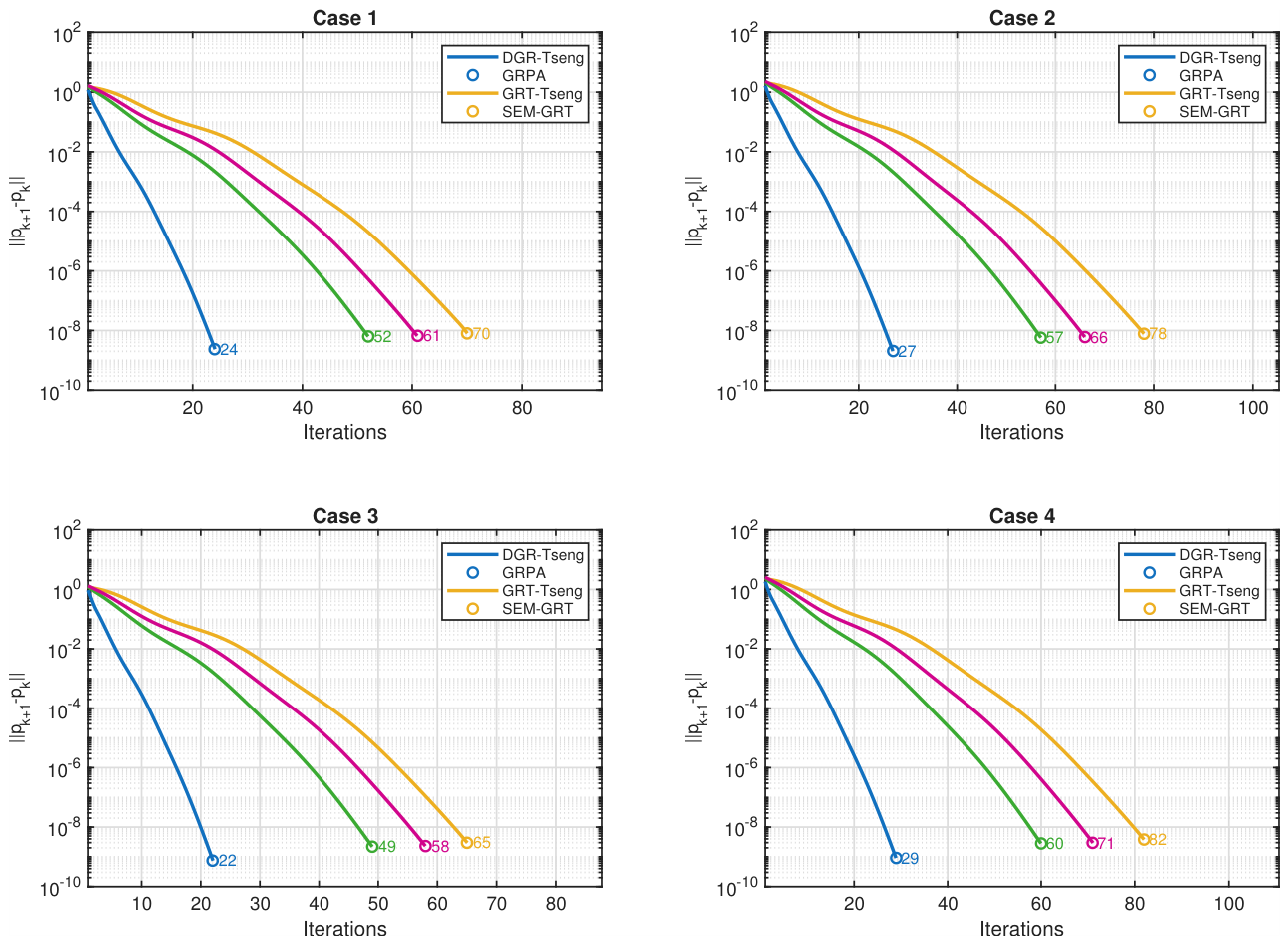
Figure 2.
Iteration-count comparison for Example 2.
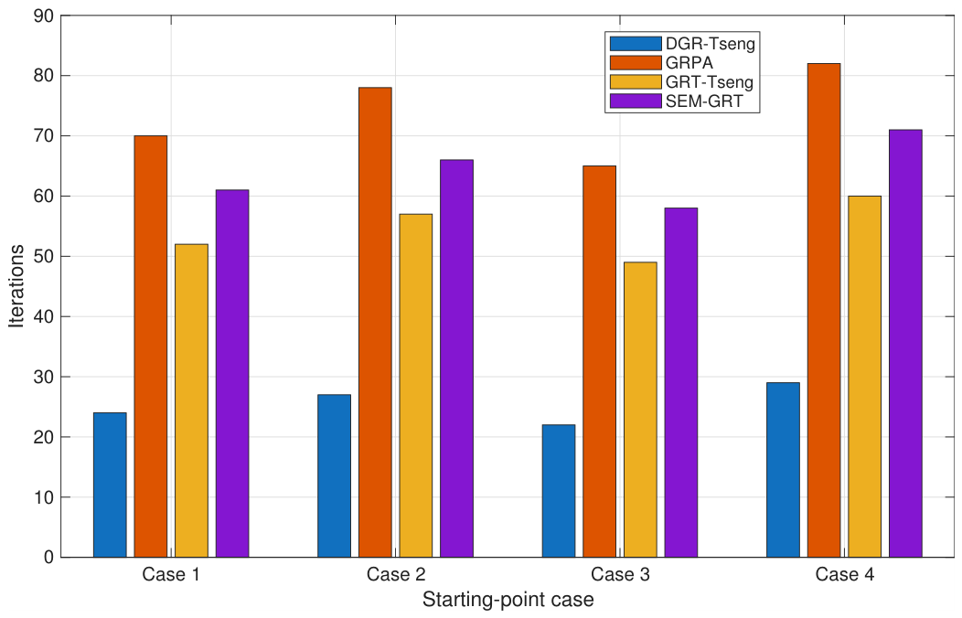
Figure 3.
CPU-time comparison for Example 2.
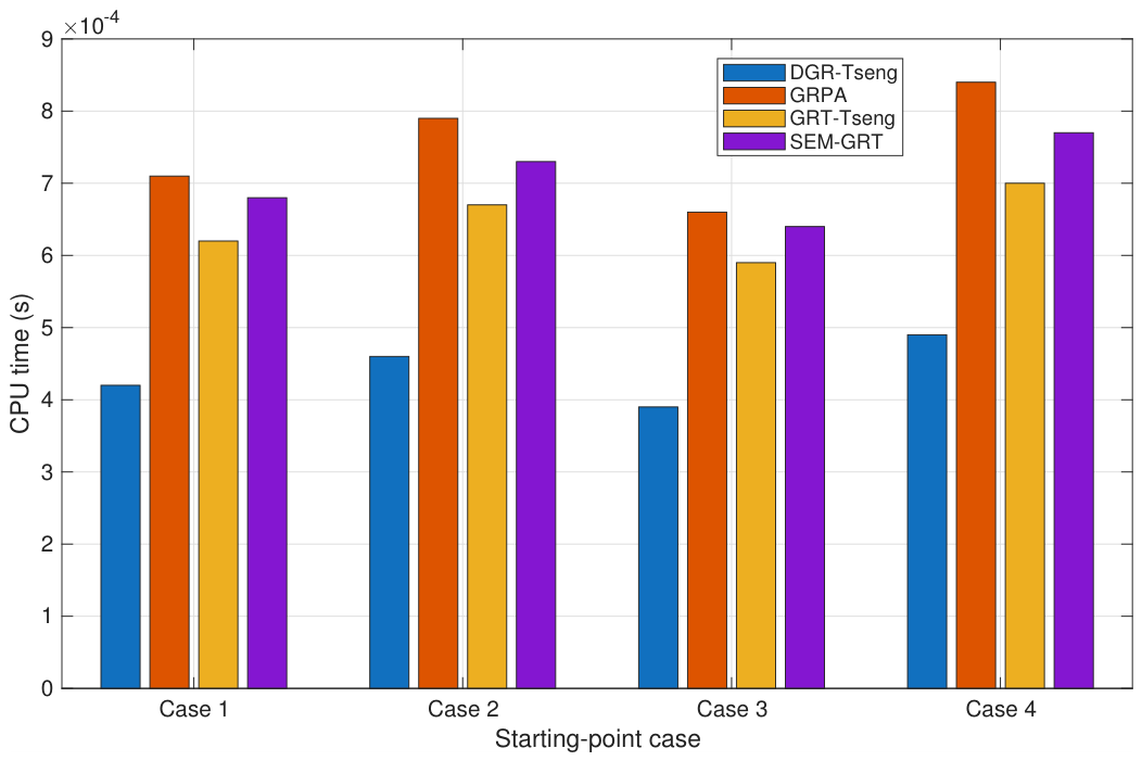
Figure 4.
Convergence profiles of the four methods for Example 3. The vertical axis represents on a logarithmic scale.
Figure 4.
Convergence profiles of the four methods for Example 3. The vertical axis represents on a logarithmic scale.
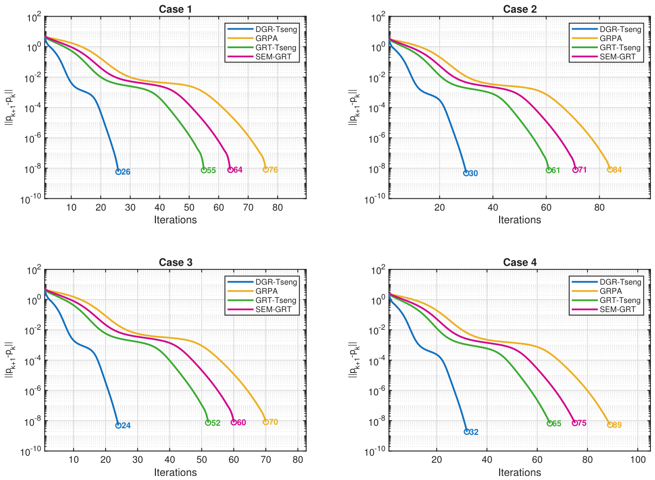
Figure 5.
Iteration-count comparison for Example 3.
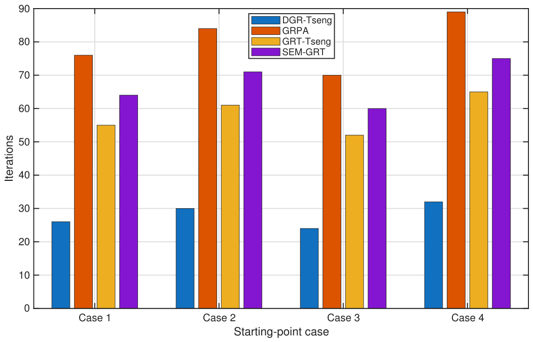
Figure 6.
CPU-time comparison for Example 3.
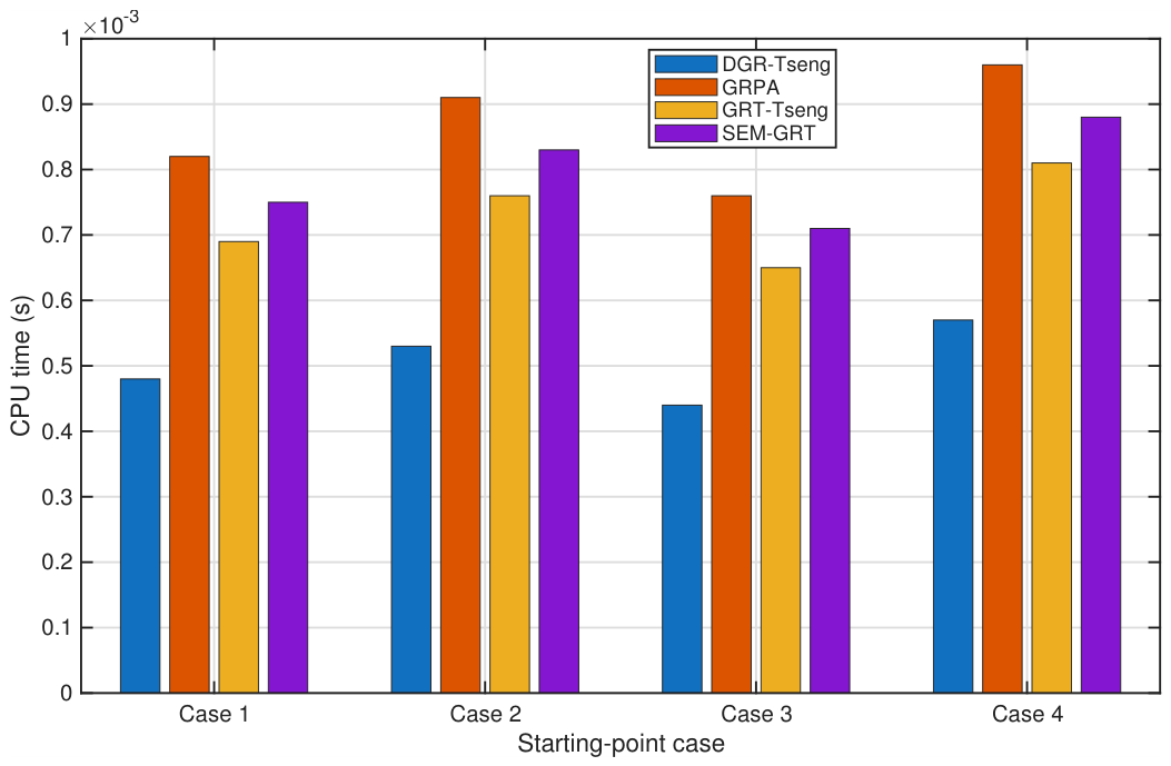
Figure 7.
Sparse signal reconstruction for .
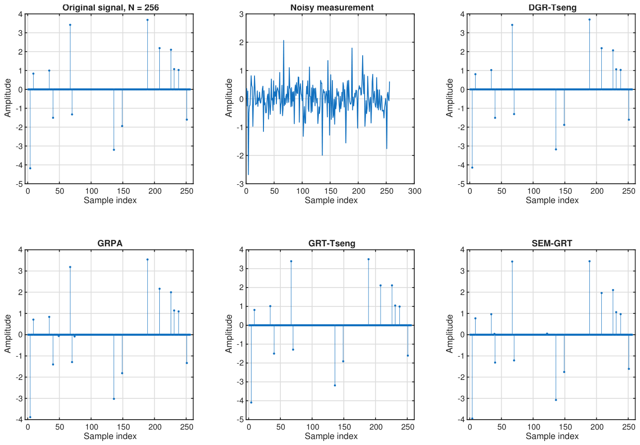
Figure 8.
Sparse signal reconstruction for .
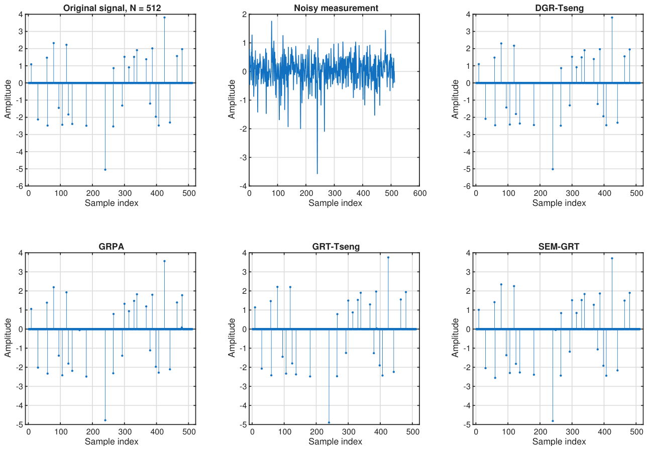
Figure 9.
Sparse signal reconstruction for .
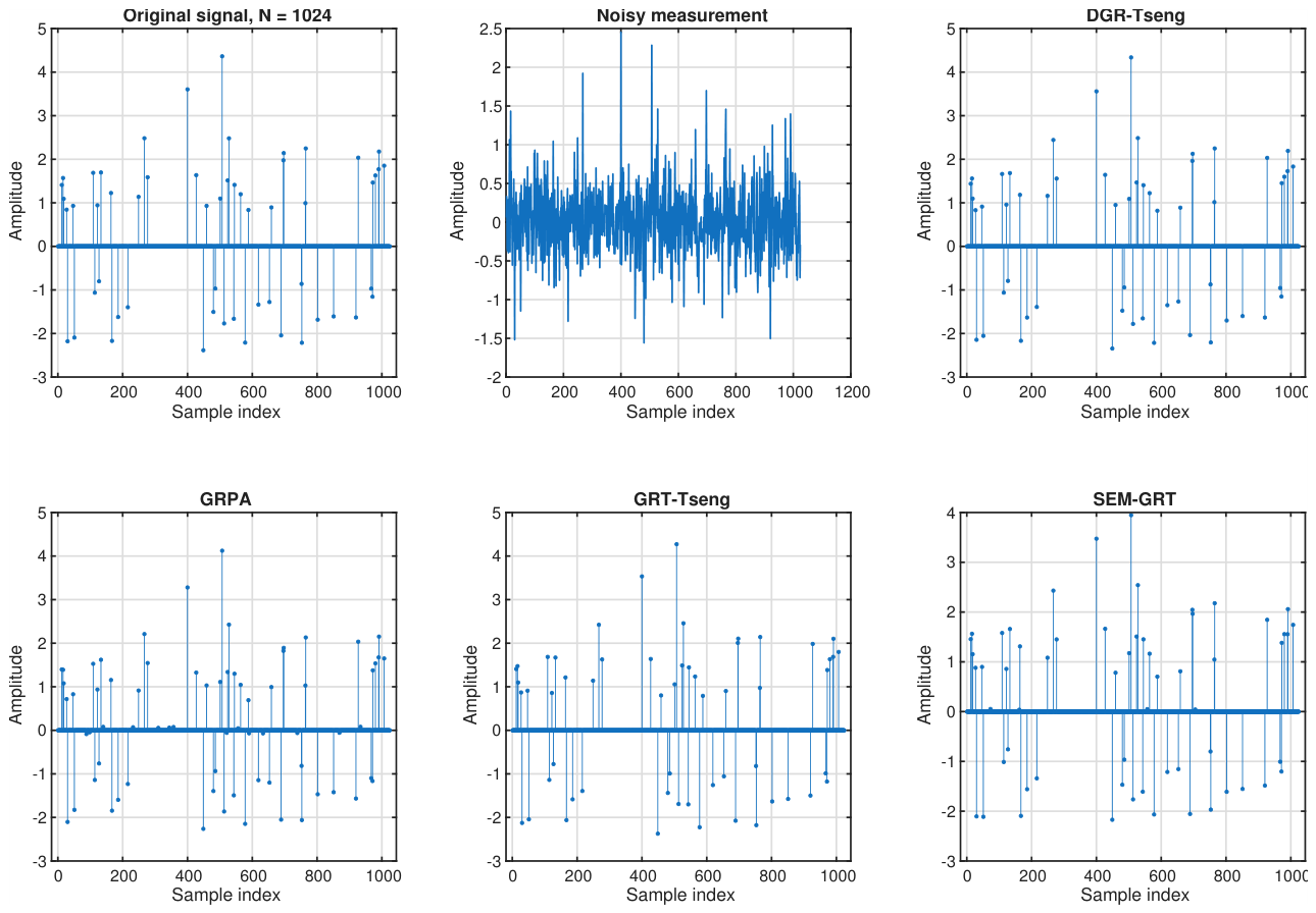
Figure 10.
Sparse signal reconstruction for .
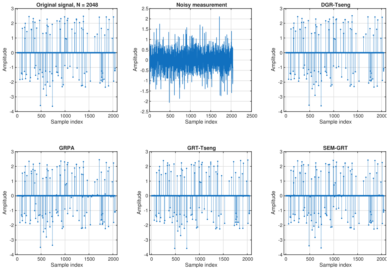
Figure 11.
MSE comparison for the four signal dimensions.
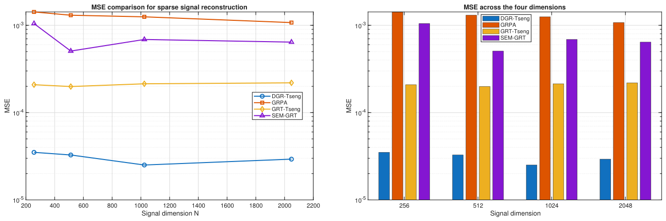
Figure 12.
SNR comparison for the four signal dimensions.
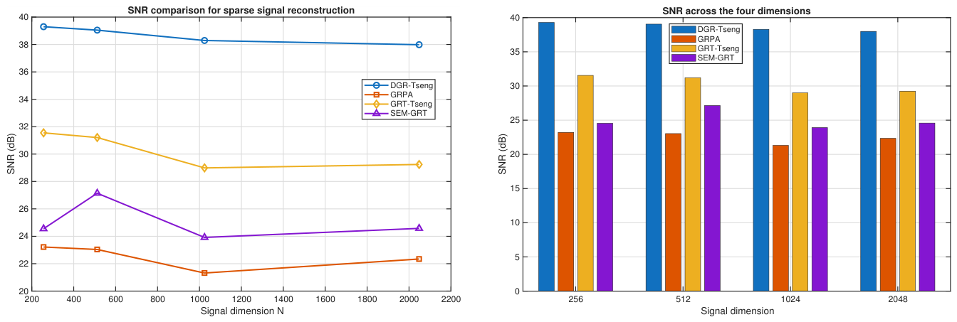
Figure 13.
Multi-OD urban traffic network with an incident-sensitive bottleneck on the link .
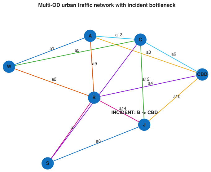
Figure 14.
The eight admissible routes associated with the two origin–destination pairs.
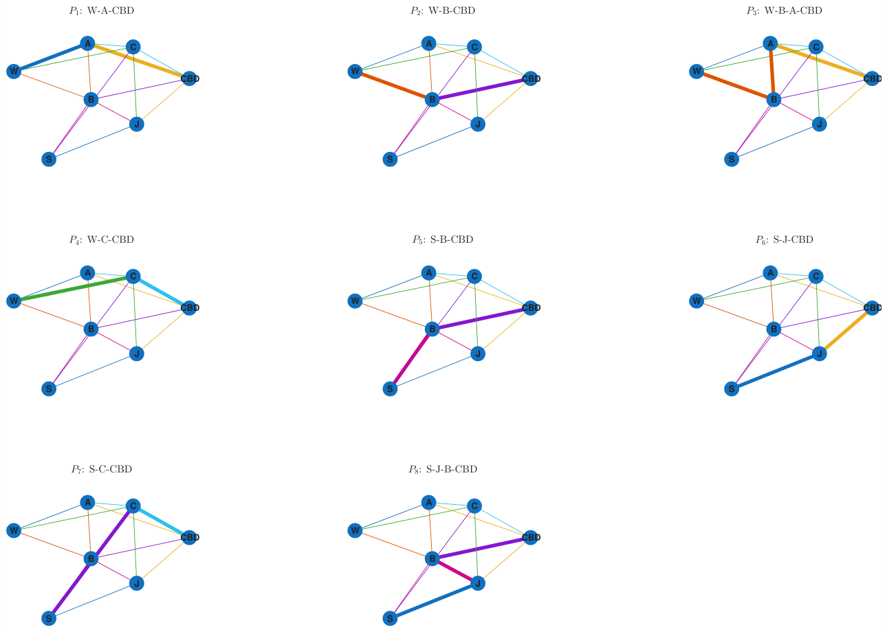
Figure 15.
Convergence profiles for Case 1: (a) natural residual ; (b) Wardrop relative gap .
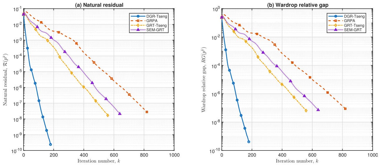
Figure 16.
Computational performance: (a) iteration counts; (b) CPU times.
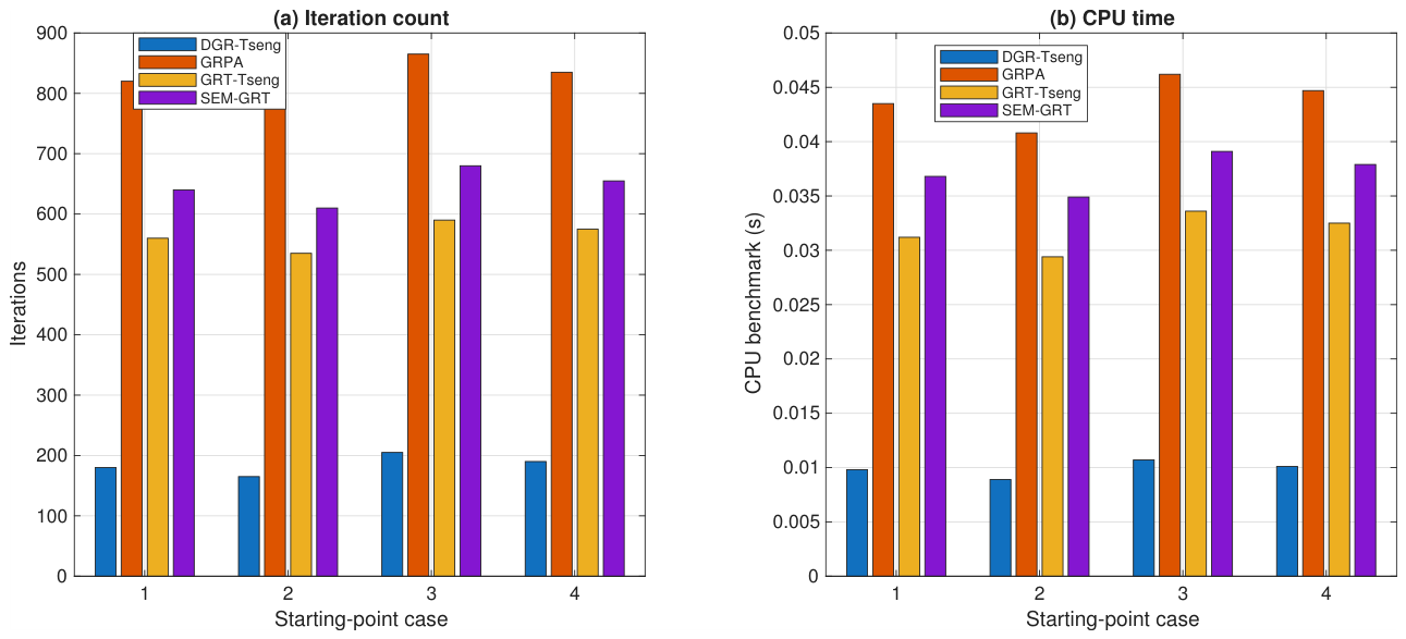
Figure 17.
Final accuracy over the four initial path-flow cases: (a) ; (b) .
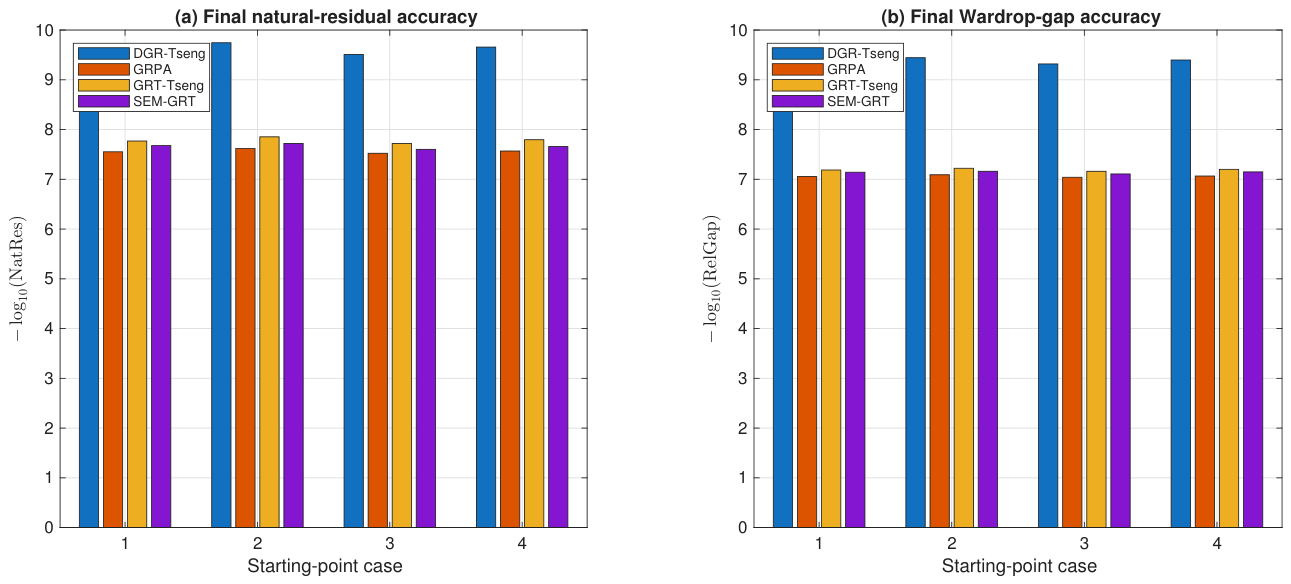
Figure 18.
Reference-based route-level sensitivity comparison: (a) route flows; (b) generalized route costs. The dashed curve represents the high-accuracy reference equilibrium.
Figure 18.
Reference-based route-level sensitivity comparison: (a) route flows; (b) generalized route costs. The dashed curve represents the high-accuracy reference equilibrium.
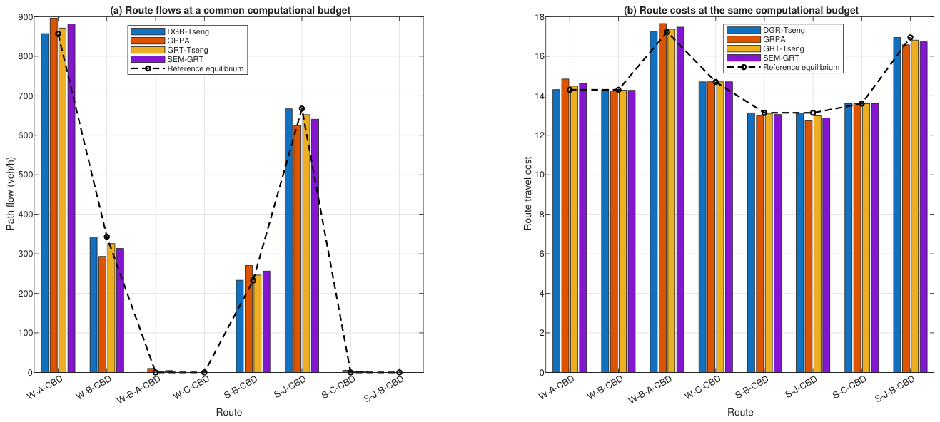
Figure 19.
Reference-based network-loading sensitivity comparison: (a) link-flow comparison; (b) link volume-to-capacity ratios. The dashed curve represents the reference equilibrium, while the horizontal dotted line in panel (b) indicates effective capacity.
Figure 19.
Reference-based network-loading sensitivity comparison: (a) link-flow comparison; (b) link volume-to-capacity ratios. The dashed curve represents the reference equilibrium, while the horizontal dotted line in panel (b) indicates effective capacity.
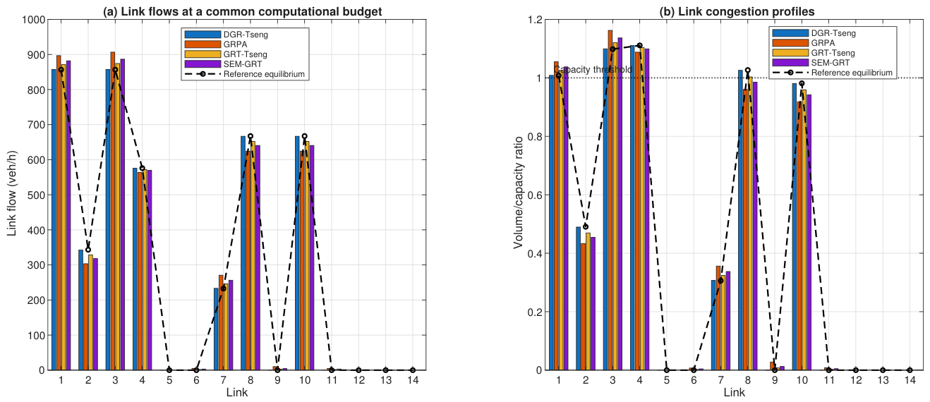
Figure 20.
Traffic-state performance over the four initial path-flow cases: (a) total system travel time; (b) maximum volume-to-capacity ratio.
Figure 20.
Traffic-state performance over the four initial path-flow cases: (a) total system travel time; (b) maximum volume-to-capacity ratio.
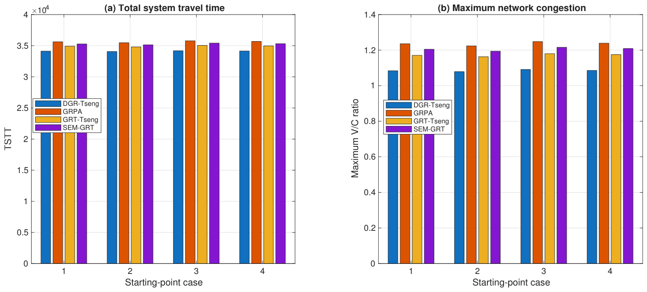

Table 1.
Control parameters used in the numerical experiments.
| Method | Control parameters |
|---|---|
| DGR-Tseng | , , , , , , . |
| GRPA | , , . |
| GRT-Tseng | , , , , . |
| SEM-GRT | , , , , . |
Table 2.
Numerical performance of the methods for Example 2.
| DGR-Tseng | GRPA | GRT-Tseng | SEM-GRT | |||||
|---|---|---|---|---|---|---|---|---|
| Case | Iter. | CPU | Iter. | CPU | Iter. | CPU | Iter. | CPU |
| 1 | 24 | 0.00042 | 70 | 0.00071 | 52 | 0.00062 | 61 | 0.00068 |
| 2 | 27 | 0.00046 | 78 | 0.00079 | 57 | 0.00067 | 66 | 0.00073 |
| 3 | 22 | 0.00039 | 65 | 0.00066 | 49 | 0.00059 | 58 | 0.00064 |
| 4 | 29 | 0.00049 | 82 | 0.00084 | 60 | 0.00070 | 71 | 0.00077 |
Note: CPU times are measured in seconds.
Table 3.
Numerical performance of the methods for Example 3.
| DGR-Tseng | GRPA | GRT-Tseng | SEM-GRT | |||||
|---|---|---|---|---|---|---|---|---|
| Case | Iter. | CPU | Iter. | CPU | Iter. | CPU | Iter. | CPU |
| 1 | 26 | 0.000480 | 76 | 0.000820 | 55 | 0.000690 | 64 | 0.000750 |
| 2 | 30 | 0.000530 | 84 | 0.000910 | 61 | 0.000760 | 71 | 0.000830 |
| 3 | 24 | 0.000440 | 70 | 0.000760 | 52 | 0.000650 | 60 | 0.000710 |
| 4 | 32 | 0.000570 | 89 | 0.000960 | 65 | 0.000810 | 75 | 0.000880 |
Note: CPU times are measured in seconds.
Table 4.
MSE and SNR performance of the competing methods for sparse signal reconstruction.
| DGR-Tseng | GRPA | GRT-Tseng | SEM-GRT | |||||
|---|---|---|---|---|---|---|---|---|
| N | MSE | SNR (dB) | MSE | SNR (dB) | MSE | SNR (dB) | MSE | SNR (dB) |
| 256 | 39.300 | 23.217 | 31.553 | 24.551 | ||||
| 512 | 39.050 | 23.039 | 31.210 | 27.145 | ||||
| 1024 | 38.294 | 21.321 | 28.993 | 23.916 | ||||
| 2048 | 37.986 | 22.342 | 29.244 | 24.578 | ||||
Table 5.
Link data for the multi-OD traffic network.
| Link | Connection | (veh/h) | |
|---|---|---|---|
| 5.0 | 850 | ||
| 5.8 | 700 | ||
| 7.0 | 780 | ||
| 6.5 | 720 | ||
| 7.5 | 650 | ||
| 7.2 | 700 | ||
| 4.8 | 760 | ||
| 5.4 | 650 | ||
| 2.5 | 360 | ||
| 6.0 | 680 | ||
| 6.4 | 620 | ||
| 2.8 | 380 | ||
| 2.2 | 420 | ||
| 2.0 | 400 |
Table 6.
Performance comparison for the multi-OD incident traffic equilibrium problem.
| Case | Method | Iter. | CPU | NatRes | RelGap | TSTT | MaxVC |
|---|---|---|---|---|---|---|---|
| 1 | DGR–Tseng | 180 | 0.0098 | 34120 | 1.084 | ||
| GRPA | 820 | 0.0435 | 35630 | 1.236 | |||
| GRT–Tseng | 560 | 0.0312 | 34920 | 1.171 | |||
| SEM–GRT | 640 | 0.0368 | 35270 | 1.205 | |||
| 2 | DGR–Tseng | 165 | 0.0089 | 34060 | 1.079 | ||
| GRPA | 790 | 0.0408 | 35480 | 1.224 | |||
| GRT–Tseng | 535 | 0.0294 | 34810 | 1.163 | |||
| SEM–GRT | 610 | 0.0349 | 35140 | 1.194 | |||
| 3 | DGR–Tseng | 205 | 0.0107 | 34190 | 1.091 | ||
| GRPA | 865 | 0.0462 | 35790 | 1.248 | |||
| GRT–Tseng | 590 | 0.0336 | 35050 | 1.180 | |||
| SEM–GRT | 680 | 0.0391 | 35410 | 1.216 | |||
| 4 | DGR–Tseng | 190 | 0.0101 | 34140 | 1.086 | ||
| GRPA | 835 | 0.0447 | 35680 | 1.239 | |||
| GRT–Tseng | 575 | 0.0325 | 34970 | 1.175 | |||
| SEM–GRT | 655 | 0.0379 | 35320 | 1.209 |
Disclaimer/Publisher’s Note: The statements, opinions and data contained in all publications are solely those of the individual author(s) and contributor(s) and not of MDPI and/or the editor(s). MDPI and/or the editor(s) disclaim responsibility for any injury to people or property resulting from any ideas, methods, instructions or products referred to in the content. |
© 2026 by the authors. Licensee MDPI, Basel, Switzerland. This article is an open access article distributed under the terms and conditions of the Creative Commons Attribution (CC BY) license (http://creativecommons.org/licenses/by/4.0/).
Copyright: This open access article is published under a Creative Commons CC BY 4.0 license, which permit the free download, distribution, and reuse, provided that the author and preprint are cited in any reuse.