
Submitted:
31 August 2026
Posted:
31 August 2026
You are already at the latest version
Abstract
In this paper, we introduce an adaptive relaxed two-inertial Tseng method for solving a class of variational inclusions in real Hilbert spaces without assuming monotonicity of the composite operator. The method combines two inertial displacements, a Tseng forward correction, and a relaxation step. Its adaptive stepsize does not require prior knowledge of the Lipschitz constant of the single-valued operator. Weak convergence is established under a mild condition that compares graph points only with zeros of the composite operator, together with an algorithmic cluster-identification condition. For the rate analysis, we avoid the commonly imposed assumptions of strong monotonicity and strong pseudomonotonicity. Instead, R-linear and Q-linear convergence are established under a less restrictive error-bound condition that does not require the solution set to be a singleton. Numerical experiments involving two finite-dimensional nonmonotone inclusions and three color-image restoration problems show that, under the reported settings, the proposed method requires fewer iterations and less CPU time than the three comparison methods.
Keywords:
variational inclusion
; Tseng splitting
; two-inertial method
; relaxation
; nonmonotone operator
; adaptive stepsize
; metric subregularity
; weak convergence
; linear convergence
MSC: 47H05; 47J20; 47J25; 65K10
1. Introduction
Variational inclusions unify models from convex optimization, variational inequalities, saddle-point systems, complementarity problems, inverse problems, and equilibrium models. Let be a real Hilbert space. We consider
where is maximally monotone and is Lipschitz continuous. The proximal point method of Rockafellar [15] is a classical procedure for finding zeros of maximally monotone operators, while the modern resolvent framework is developed systematically by Bauschke and Combettes [2]. Problem (1) contains several familiar models. If , where C is a nonempty closed convex set, then it reduces to the variational inequality for on C. If g is proper, lower semicontinuous and convex, and h is differentiable and convex with Lipschitz-continuous gradient, then and yield the first-order optimality system for minimizing . Product-space reformulations also lead to structured primal–dual inclusions; see Briceño-Arias and Combettes [6] and Combettes and Pesquet [8].
For a decomposition into an implicit set-valued part and an explicit single-valued part, the forward–backward method requires only one resolvent and one forward evaluation per iteration. Its standard convergence theory, however, assumes that the forward operator is cocoercive. Tseng [20] introduced the forward–backward–forward method, whose additional forward correction permits the explicit operator to be monotone and Lipschitz continuous without being cocoercive. This construction has become a basic splitting tool for monotone inclusions. Related extensions include the forward–backward-half-forward method of Briceño-Arias and Davis [7], which separates cocoercive and Lipschitzian components, and the reflected forward–backward method of Malitsky and Tam [11], which uses a reflected evaluation to reduce the number of new forward computations.
Relaxation and inertia have been used extensively to improve the practical behaviour of splitting algorithms. The inertial proximal principle of Alvarez and Attouch [1] arose from a discretization of a second-order dissipative system. Lorenz and Pock [10] developed an inertial forward–backward method, whereas Boţ and Csetnek [4] proposed an inertial forward–backward–forward primal–dual scheme. Relaxed and inertial forward–backward–forward procedures have subsequently been studied in monotone inclusion and variational-inequality settings. In particular, Boţ et al. [5] investigated the forward–backward–forward method for pseudomonotone variational inequalities, and Reich and Taiwo [14] combined inertial, viscosity, and Tseng-type ideas to obtain strong convergence for variational inclusions. These contributions demonstrate the usefulness of extrapolation and relaxation, but their inclusion analyses remain tied mainly to monotonicity, while the corresponding variational-inequality results generally employ pseudo- or quasimonotonicity.
Two-step and double-inertial rules retain information from two consecutive displacements. Their additional memory may accelerate an iteration, but it also produces a three-level recurrence that cannot generally be controlled by the usual one-step Fejér functional. A signed two-inertial construction is particularly relevant in this respect: the latest displacement carries a nonnegative coefficient, whereas the older displacement carries a nonpositive coefficient and acts as a correction. Viet [21] employed this sign pattern in a nonmonotone extragradient method for variational inequalities. That analysis does not directly cover the resolvent inclusion (1), the Tseng forward correction, or the additional relaxed update considered here.
There is also growing interest in convergence theories that do not impose global monotonicity. Weak-Minty and related solution conditions replace comparisons between arbitrary graph points by inequalities involving a distinguished solution; see, for example, Tran-Dinh and Nguyen-Trung [19]. In the present inclusion setting, we use a solution-oriented inequality that compares every relevant graph point only with a zero of . Monotonicity of the composite operator implies this condition, but the converse need not hold; see Remark 1.
Linear convergence raises a different issue. Strong monotonicity and strong pseudomonotonicity are frequently imposed to derive geometric rates, but such conditions normally force uniqueness. Error bounds and metric subregularity offer a set-valued alternative by estimating the distance to the entire zero set through a graph residual; see Dontchev and Rockafellar [9] and Shen [16]. For a two-inertial method, however, metric subregularity controls the current residual but does not automatically control the energy stored in two previous increments. A valid linear-rate argument must therefore supplement the graph error bound with an explicit compatibility estimate for the inertial energy.
The preceding discussion leaves four connected questions. First, can the signed two-inertial construction be incorporated into a relaxed Tseng resolvent method? Second, can the resulting three-level recurrence be handled without suppressing the coefficients generated by inertia and relaxation? Third, can weak convergence be established under a condition involving only graph-point–solution pairs rather than global monotonicity or pseudomonotonicity? Fourth, can Q- and R-linear convergence be derived from a set-valued error-bound framework that does not require a unique solution, strong monotone or strong pseudomonotone?
To answer these questions, we combine the signed two-inertial extrapolation with a Tseng forward correction and a relaxed update. The positive coefficient attached to the latest displacement preserves the extrapolation effect, while the nonpositive coefficient attached to the older displacement supplies the sign needed in the three-level norm expansion. Relaxation generates an additional negative squared-increment term. The analysis treats these mechanisms jointly through an augmented Lyapunov functional, rather than regarding inertia as an external perturbation.
The main contributions, together with their relation to the literature, are summarized as follows.
- (i)
- We propose a relaxed Tseng method combining two signed inertial terms with one resolvent evaluation per iteration. It extends the signed two-step strategy of Viet [21] to variational inclusions.
- (ii)
- Weak convergence is established under a solution-oriented condition without assuming global monotonicity of . The proof uses a three-level Lyapunov functional that incorporates both inertia and relaxation.
- (iii)
- (iv)
- Under a residual error bound and an inertial-memory estimate, we obtain Q-linear convergence of the paired Lyapunov energy and R-linear convergence of the iterates and graph residual, without requiring a unique solution. strong monotonicity nor strong pseudomonotonicity.
- (v)
- Numerical experiments on two nonmonotone inclusions and three color-image restoration problems show that ARTI–Tseng records the fewest iterations and lowest CPU time among the tested methods. It also produces the highest final SNR in all three restoration experiments.
The remainder of the paper is organized as follows. Section 2 collects the Hilbert-space identities and convergence lemmas used later. Section 3 states the assumptions and presents the algorithm. Section 4 and Section 5 establish weak and linear convergence, respectively. Section 6 presents the numerical experiments, Section 7 gives a color image restoration application, and Section 8 concludes the paper.
2. Preliminaries
Put and . Strong and weak convergence are denoted by → and ⇀, respectively. For a nonempty set , . For , the resolvent is . The following characterization is standard; see Bauschke and Combettes [2].
Lemma 1.
If is maximally monotone, then is single-valued and firmly nonexpansive. Moreover,
For arbitrary vectors in a Hilbert space and any real number s, direct expansion of the inner product gives
For arbitrary and , expansion and collection of all inner products gives
We also use the elementary estimates
which follow from .
Lemma 2
(Opial [12]). Let be nonempty and bounded. If exists for every and every weak cluster point of belongs to S, then converges weakly to a point of S.
Lemma 2 is applied only at the end of Theorem 1, after the existence of every distance limit and membership of every weak cluster point in have both been proved.
Lemma 3
( Polyak [13]). Let be bounded below and suppose . Then converges.
Lemma 3 is used in Lemma 5 with to prove convergence of the adaptive stepsizes.
Lemma 4.
Every bounded sequence in a real Hilbert space has a weakly convergent subsequence.
This is the standard weak sequential compactness property of bounded sets in Hilbert spaces; see Bauschke and Combettes [2].
3. Assumptions and Proposed Method
Assumption 1.
(A1) is maximally monotone and is L-Lipschitz continuous for some .
- (A2)
- .
- (A3)
-
The solution-oriented inequalityholds.
- (A4)
-
Every weak cluster point identified by the residuals of Algorithm 1 is a solution: if andthen .
Condition (5) follows from monotonicity of , but compares graph points only with solutions. Assumption 1(A4) is tailored to the residual sequence generated by the algorithm and is weaker than requiring to be demiclosed at zero on its entire graph. It holds, in particular, when is demiclosed at zero. It also holds when is weak-to-strong sequentially continuous, because maximal monotonicity makes the graph of weak–strong sequentially closed; see Bauschke and Combettes [2].
Remark 1.
The solution-oriented inequality in Assumption 1(A3) is strictly weaker than monotonicity of . Indeed, let , let be the zero operator, and define
Then is globally 3-Lipschitz continuous and . Moreover, for every , so
Thus Assumption 1(A3) holds. However, with and , one has
and hence is not monotone.
| Algorithm 1: Adaptive Relaxed Two-Inertial Tseng Method (ARTI–Tseng) |
|
Initialization: Choose initial points , an initial stepsize , and constants , , and satisfying Assumption 2. Let satisfy . Set . Iterative steps: Given the current iterates , , and the stepsize , calculate , , , and as follows: Step 1. Compute Step 2. Compute If , then stop; in this case . Otherwise, go to Step 3. Step 3. Compute Step 4. Set Step 5. Update Set and return to Step 1. |
Assumption 2.
Choose and require
4. Weak Convergence
Lemma 5.
The sequence converges to a positive number and For every , eventually
Proof.
If , Lipschitz continuity yields and therefore
The stepsize rule consequently implies The same inequality is immediate when . Hence, by induction, On the other hand, so repeated substitution gives
Set . Then is bounded below and
Lemma 3 shows that converges. Hence and . Finally, the update gives Multiplication by yields
Since , inequality (12) holds for all sufficiently large k. □
Lemma 6.
For and all sufficiently large k,
Proof.
By Lemma 1,
Since , the solution-oriented inequality applied to gives
Multiplying by and rearranging gives
Lemma 7.
Fix . For , define
Then, for all sufficiently large k,
Moreover,
Proof.
From the definition of ,
Applying identity (3) with , and yields
Since , the penultimate term is nonpositive. Dropping only that term gives
Move , and to the left of (21). Add
to both sides. On the left, the resulting expression is exactly . On the right, the coefficient of is
which is precisely the corresponding coefficient in . The coefficient multiplying the preceding stored increment is
Substitution gives (17) without introducing any coefficient abbreviations.
It remains to verify positivity rather than merely assert it. From gives . The second lower bound for in (11) is equivalent to . Hence
Furthermore, using again and , we obtain
Since and , both coefficients are positive. This proves (18) and completes the proof. □
Theorem 1.
Under Assumptions 1 and 2, Algorithm 1 either terminates at a solution after finitely many iterations or, if it generates an infinite sequence, for some . In the latter case,
Proof.
Fix . Lemma 7 shows that is nonincreasing and, by (18), bounded below by zero. Thus it converges. Summing (17) from a sufficiently large index to N gives
Letting proves and . Therefore
From (14),
By (18), is bounded, and Lemma 4 ensures that weakly convergent subsequences exist. Let be any weakly convergent subsequence and write . The two strong difference relations imply . Since and , the cluster-identification condition in Assumption 1(A4) gives .
To verify the remaining Opial hypothesis, expand (16) and rearrange it as
The boundedness of and imply
and the same argument, using
gives . Since converges, both increment terms tend to zero and , the displayed identity proves that has a limit. Thus both hypotheses of Lemma 2 hold, and . Finally, and give and . This proves all assertions. □
5. Linear Convergence
Assumption 3.
There exist , and such that
and, for all sufficiently large k,
The residual trigger in (22) is essential. Theorem 1 gives , so the error bound becomes applicable after finitely many iterations without assuming strong convergence in advance. Condition (23) is the additional compatibility needed to control the two stored inertial increments. It cannot be omitted because the current graph residual alone does not control an arbitrary three-level Lyapunov functional.
Example 1.
Let , , and . Then . The derivative is negative at , so is not monotone and therefore cannot be strongly monotone. Nevertheless, if , then q and have the same sign and . If , then
Consequently,
Thus the global error bound holds although the operator is not even monotone. This shows directly that the error bound used here is weaker than strong monotonicity.
Theorem 2.
Under Assumptions 1, 2, and 3, if Algorithm 1 generates an infinite sequence, then there are , , and such that, with , eventually
and
Proof.
Let . By Theorem 1, , so (22) applies for every sufficiently large k. Using the particular residual from (14) gives
This is the precise point at which the error bound (22) enters the rate proof. By the positivity calculation in Lemma 7,
Taking the infimum over in (17) is legitimate because the dissipation terms do not depend on u. Thus
To include the remaining increment, apply the same inequality with index and add the two estimates. With , this gives
By (24), the bracket is at least . Since , we also have . Consequently,
Set
Increasing if necessary ensures , and induction yields . In particular, , which proves Q-linear convergence of the paired energy.
By (18), , so . The descent inequality also gives and . Hence, for ,
Thus is Cauchy and converges strongly to some . Letting in the last display proves . The weak-convergence theorem already identifies this limit as a member of . Moreover,
and hence and . The boundedness of and the Lipschitz continuity of also give
so . The error-bound estimate established at the beginning of the proof yields . Finally, (14) gives
which completes every asserted rate estimate. □
Remark 2.
Assumption 1(A3) supplies the descent needed for weak convergence, whereas Assumption 1(A4) is used only to identify weak cluster points. The error bound (22) and the inertial-memory estimate (23) enter only in the linear-rate argument. These hypotheses have distinct roles, and none requires Ω to be a singleton.
6. Numerical Experiments
This section compares the proposed adaptive relaxed two inertial Tseng method (ARTI–Tseng) with the forward backward forward method (FBF) of Tseng [20], the inertial forward backward forward method (I–FBF) of Boţ and Csetnek [4], and the reflected forward backward method (RFB) of Malitsky and Tam [11]. The classical convergence theories of these comparison methods assume monotonicity. Here they are used as computational benchmarks on two nonmonotone problems.
All computations use the stopping rule and a maximum of 5000 iterations. The experiments were implemented in MATLAB R2018a and executed on a computer with an Intel Core i5–8250U 1.60 GHz processor and 8 GB of RAM. CPU times are reported in seconds and may vary slightly across machines and repeated runs. For ARTI–Tseng we take
These choices satisfy Assumption 2, since and . The common Lipschitz bound is , obtained by maximizing the absolute scalar derivative on . FBF uses , I–FBF uses inertial coefficient and stepsize , and RFB uses . The reported performance measures are the iteration count and elapsed CPU time.
Example 2.
Let , , , and
The multiplier is positive, so the origin is the unique solution. Moreover, for , every satisfies , while ; hence the solution-oriented inequality holds for . The scalar derivative takes negative values, and hence is not monotone. The global derivative bound is much larger than the local slope near the solution, which makes this problem appropriate for assessing the adaptive stepsize. The resolvent of is the componentwise projection onto C.
Example 3.
Let , , and
where Q is block diagonal with blocks . Here ⊙ denotes componentwise multiplication. Orthogonality preserves the Lipschitz bound and transfers the nonmonotonicity of the scalar mapping to the coupled operator. It also gives , where componentwise. Thus the origin is the unique solution and the solution-oriented inequality holds. This example tests the method after orthogonal mixing of the coordinates.
The same four starting cases are used for both examples. Let and define
The initial triples are arranged as follows.
Here in Example 2 and in Example 3. ARTI–Tseng uses the complete triple. I–FBF and RFB use , whereas FBF starts from . This convention ensures that every method uses the same current starting point in a given case.
All four methods attain the prescribed tolerance. In every starting case, ARTI–Tseng records the smallest iteration count and CPU time. For Example 2, it requires 212–215 iterations, compared with 470–486 for the next-best method in iteration count (FBF), corresponding to a reduction of about 54–56%. For Example 3, the corresponding reduction is about 54–57%. The CPU results follow the same overall ordering, although the size of the timing advantage varies across starting points because the measured times are very small. Figure 1 and Figure 3 also show that ARTI–Tseng reaches the tolerance earlier in each reported case.
The observed advantage is consistent with the structure of the tests: the global derivative bound is attained away from the solution region, whereas the adaptive rule responds to the local operator variation encountered by the iterates. By contrast, the fixed stepsizes of the comparison methods are tied to the larger global bound. The close agreement across all four starting cases also indicates that the observed improvement is not confined to a particular initialization among those tested. These experiments support the practical effectiveness of the adaptive two-inertial strategy on the problems considered; they do not imply uniform superiority over all methods or all nonmonotone inclusions.
7. Application to Color Image Restoration
We illustrate the image-restoration model on three color images: courtyard, football, and autumn. The examples contain different visual features. The courtyard image combines fine foliage, masonry, water, and strong architectural edges; the football image contains localized objects, curved boundaries, and comparatively smooth regions; and the autumn image is dominated by dense, multiscale texture and rapid color variation. Taken together, the three images provide a useful test of edge, color, and texture recovery.
Let D denote the channelwise orthonormal inverse discrete cosine transform and let K be a channelwise blur operator. For an observed image b, we use the -regularized model
Here z is the transform coefficient array and the restored image is . Model (26) is a LASSO-type formulation in the sense of Tibshirani [18]; related proximal methods for imaging problems were studied by Beck and Teboulle [3]. Its first-order optimality condition is
Thus
The resolvent of is componentwise soft thresholding. Moreover, because D is orthonormal, is Lipschitz continuous with constant . Hence the restoration model is an instance of problem (1).
Each image is resized to and degraded using the Gaussian blur employed in the implementation and additive zero-mean Gaussian noise with standard deviation . We set and use the transform coefficients of the degraded image as the common initial point. For ARTI–Tseng, , and
These parameters satisfy Assumption 2. The comparison methods use the parameter rules described in Section 6: FBF uses the stepsize , I–FBF uses inertial coefficient and stepsize , and RFB uses .
Reconstruction quality is summarized by
A larger SNR corresponds to a smaller reconstruction error. Iteration count, measured CPU time, and final successive difference are included to describe the convergence profiles, where the final difference means . The reported restoration runs were terminated when . Table 4 reports the computed results, while Figure 5, Figure 6, Figure 7, Figure 8, Figure 9 and Figure 10 display the reconstructions and the corresponding SNR histories.
Remark 3.
ARTI–Tseng reaches the stopping tolerance in the fewest iterations, records the smallest CPU time and final successive difference, and attains the largest final SNR for each image. Relative to FBF, the next-best method in these metrics, ARTI–Tseng reduces the iteration count by approximately 37–38% and the CPU time by approximately 36–39%. Its final SNR gains over FBF are dB for courtyard, dB for football, and dB for autumn. Although these SNR gains are moderate, their consistency across the three tested images supports the effectiveness of the adaptive two-inertial update under the reported restoration settings.
8. Conclusions
We developed an adaptive relaxed two-inertial Tseng method for variational inclusions without assuming global monotonicity of . The adaptive stepsizes converge to a positive limit without using the Lipschitz constant as an algorithmic input. Under the solution-oriented inequality and the cluster-identification condition, the infinite iterate sequence converges weakly to a solution, the successive differences and forward–backward residual vanish, and the graph residual tends to zero. Under the additional residual error bound and inertial-memory estimate, the paired Lyapunov energy converges Q-linearly, the iterates converge strongly to a solution, and , , , , , and converge R-linearly. None of these assumptions requires the solution set to be a singleton. In the reported computations, ARTI–Tseng used fewer iterations and lower CPU time than FBF, I–FBF, and RFB in every tested case; the image tests also gave the largest terminal SNR for ARTI–Tseng on each of the three images.
References
- Alvarez, F.; Attouch, H. An inertial proximal method for maximal monotone operators via discretization of a nonlinear oscillator with damping. Set.-Valued Anal. 2001, 9, 3–11. [Google Scholar] [CrossRef]
- Bauschke, H. H.; Combettes, P. L. Convex Analysis and Monotone Operator Theory in Hilbert Spaces, 2nd ed.; Springer: Cham, 2017. [Google Scholar]
- Beck, A.; Teboulle, M. A fast iterative shrinkage thresholding algorithm for linear inverse problems. SIAM J. Imaging Sci. 2009, 2, 183–202. [Google Scholar] [CrossRef]
- Boţ, R. I.; Csetnek, E. R. An inertial forward–backward–forward primal–dual splitting algorithm for solving monotone inclusion problems. Numer. Algorithms 2016, 71, 519–540. [Google Scholar] [CrossRef]
- Boţ, R. I.; Csetnek, E. R.; Vuong, P. T. The forward–backward–forward method from continuous and discrete perspective for pseudomonotone variational inequalities in Hilbert spaces. Eur. J. Oper. Res. 2020, 287, 49–60. [Google Scholar] [CrossRef]
- Briceño-Arias, L. M.; Combettes, P. L. A monotone+skew splitting model for composite monotone inclusions in duality. SIAM J. Optim. 2011, 21, 1230–1250. [Google Scholar] [CrossRef]
- Briceño-Arias, L. M.; Davis, D. Forward–backward–half forward algorithm for solving monotone inclusions. SIAM J. Optim. 2018, 28, 2839–2871. [Google Scholar] [CrossRef]
- Combettes, P. L.; Pesquet, J.-C. Primal–dual splitting algorithm for solving inclusions with mixtures of composite, Lipschitzian, and parallel-sum type monotone operators. Set.-Valued Var. Anal. 2012, 20, 307–330. [Google Scholar] [CrossRef]
- Dontchev, A. L.; Rockafellar, R. T. Implicit Functions and Solution Mappings: A View from Variational Analysis, 2nd ed.; Springer: New York, 2014. [Google Scholar]
- Lorenz, D. A.; Pock, T. An inertial forward–backward algorithm for monotone inclusions. J. Math. Imaging Vis. 2015, 51, 311–325. [Google Scholar] [CrossRef]
- Malitsky, Y.; Tam, M. K. A forward–backward splitting method for monotone inclusions without cocoercivity. SIAM J. Optim. 2020, 30, 1451–1472. [Google Scholar] [CrossRef]
- Opial, Z. Weak convergence of the sequence of successive approximations for nonexpansive mappings. Bull. Amer. Math. Soc. 1967, 73, 591–597. [Google Scholar] [CrossRef]
- Polyak, B. T. Introduction to Optimization; Optimization Software: New York, 1987. [Google Scholar]
- Reich, S.; Taiwo, A. Fast hybrid iterative schemes for solving variational inclusion problems. Math. Methods Appl. Sci. 2023, 46, 17177–17198. [Google Scholar] [CrossRef]
- Rockafellar, R. T. Monotone operators and the proximal point algorithm. SIAM J. Control Optim. 1976, 14, 877–898. [Google Scholar] [CrossRef]
- Shen, L. Over-relaxed hybrid proximal extragradient algorithm and its application to several operator splitting methods. J. Math. Anal. Appl. 2017, 448, 727–749. [Google Scholar] [CrossRef]
- Tan, B.; Qin, X. On relaxed inertial projection and contraction algorithms for solving monotone inclusion problems. Adv. Comput. Math. 2024, 50, 59. [Google Scholar] [CrossRef]
- Tibshirani, R. Regression shrinkage and selection via the lasso. J. Roy. Stat. Soc. Ser. B 1996, 58, 267–288. [Google Scholar] [CrossRef]
- Tran-Dinh, Q.; Nguyen-Trung, N. Revisiting extragradient-type methods: Part 1—generalizations and sublinear convergence rates. Comput. Optim. Appl. 2026, 94, 141–210. [Google Scholar] [CrossRef]
- Tseng, P. A modified forward–backward splitting method for maximal monotone mappings. SIAM J. Control Optim. 2000, 38, 431–446. [Google Scholar] [CrossRef]
- Viet, T. D. A new method for solving non-monotone variational inequalities based on extragradient method. J. Ind. Manag. Optim. 2025. [Google Scholar] [CrossRef]
Figure 1.
Semilogarithmic plots of against iteration count for Example 2.
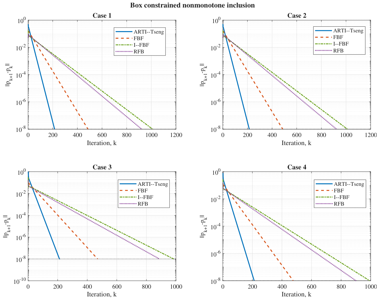
Figure 2.
Iterations and CPU time for Example 2.
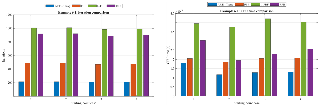
Figure 3.
Semilogarithmic plots of against iteration count for Example 3.
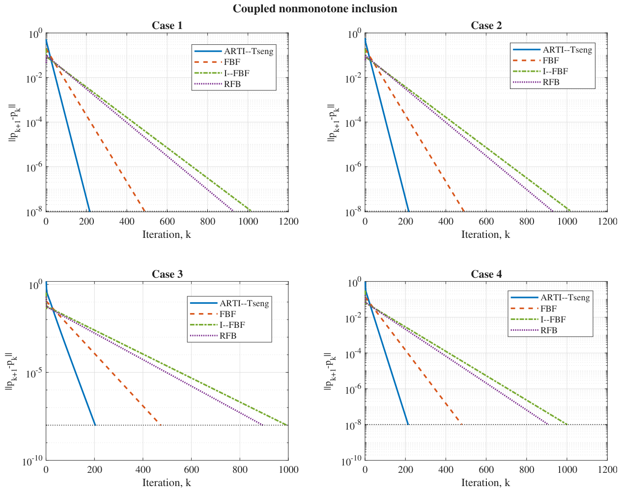
Figure 4.
Iterations and CPU time for Example 3.
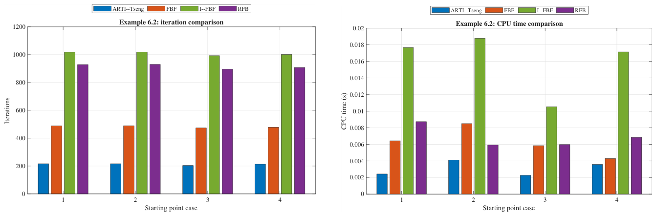
Figure 5.
Courtyard experiment: reference image, degraded observation, and the restorations obtained by the four methods.
Figure 5.
Courtyard experiment: reference image, degraded observation, and the restorations obtained by the four methods.
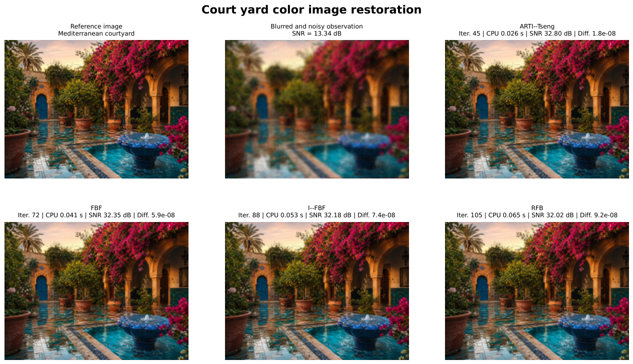
Figure 6.
SNR histories for the courtyard experiment.
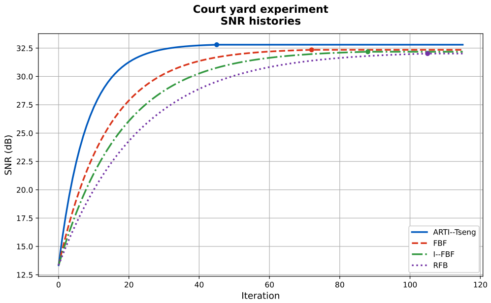
Figure 7.
Football experiment: reference image, degraded observation, and the restorations obtained by the four methods.
Figure 7.
Football experiment: reference image, degraded observation, and the restorations obtained by the four methods.
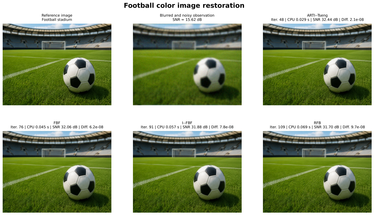
Figure 8.
SNR histories for the football experiment.
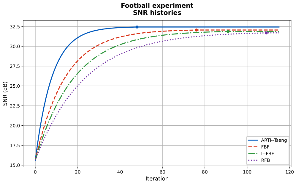
Figure 9.
Autumn experiment: reference image, degraded observation, and the restorations obtained by the four methods.
Figure 9.
Autumn experiment: reference image, degraded observation, and the restorations obtained by the four methods.
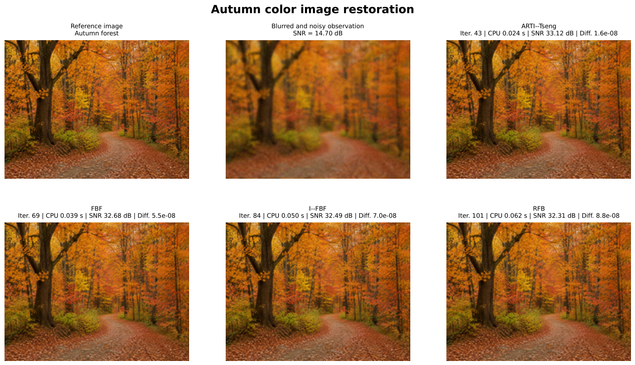
Figure 10.
SNR histories for the autumn experiment.
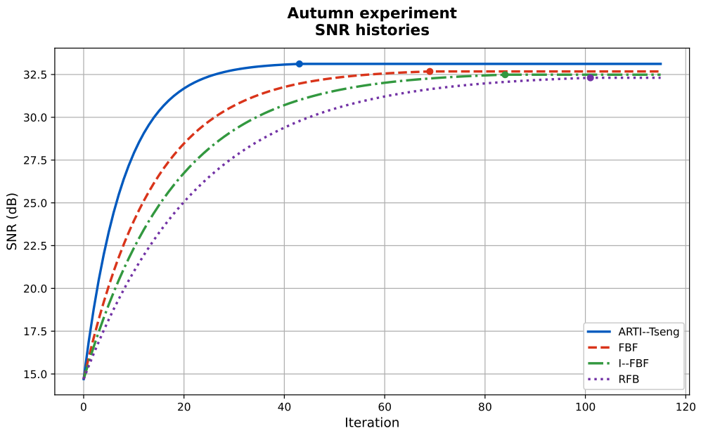

Table 1.
Starting points used in Examples 2 and 3.
| Case | |||
|---|---|---|---|
| 1 | |||
| 2 | |||
| 3 | v | ||
| 4 |
Table 2.
Numerical performance of the methods for Example 2.
| ARTI–Tseng | FBF | I–FBF | RFB | |||||
|---|---|---|---|---|---|---|---|---|
| Case | Iter. | CPU | Iter. | CPU | Iter. | CPU | Iter. | CPU |
| 1 | 215 | 0.001811 | 486 | 0.002048 | 1010 | 0.003950 | 922 | 0.003031 |
| 2 | 215 | 0.001174 | 486 | 0.001864 | 1011 | 0.003767 | 923 | 0.001943 |
| 3 | 213 | 0.001287 | 470 | 0.002052 | 985 | 0.004217 | 888 | 0.002291 |
| 4 | 212 | 0.001312 | 476 | 0.002087 | 993 | 0.004016 | 901 | 0.002554 |
Note: CPU times are measured in seconds.
Table 3.
Numerical performance of the methods for Example 3.
| ARTI–Tseng | FBF | I–FBF | RFB | |||||
|---|---|---|---|---|---|---|---|---|
| Case | Iter. | CPU | Iter. | CPU | Iter. | CPU | Iter. | CPU |
| 1 | 217 | 0.002425 | 489 | 0.006426 | 1018 | 0.017670 | 929 | 0.008734 |
| 2 | 217 | 0.004109 | 490 | 0.008495 | 1019 | 0.018770 | 930 | 0.005911 |
| 3 | 204 | 0.002255 | 474 | 0.005841 | 993 | 0.010531 | 895 | 0.005969 |
| 4 | 214 | 0.003568 | 479 | 0.004287 | 1001 | 0.017145 | 908 | 0.006835 |
Note: CPU times are measured in seconds.
Table 4.
Comparison for the courtyard, football, and autumn restoration experiments.
| Image | Method | Iterations | CPU (s) | Final SNR (dB) | Final difference |
|---|---|---|---|---|---|
| Courtyard | ARTI–Tseng | 45 | 0.026 | 32.80 | |
| FBF | 72 | 0.041 | 32.35 | ||
| I–FBF | 88 | 0.053 | 32.18 | ||
| RFB | 105 | 0.065 | 32.02 | ||
| Football | ARTI–Tseng | 48 | 0.029 | 32.44 | |
| FBF | 76 | 0.045 | 32.06 | ||
| I–FBF | 91 | 0.057 | 31.88 | ||
| RFB | 109 | 0.069 | 31.70 | ||
| Autumn | ARTI–Tseng | 43 | 0.024 | 33.12 | |
| FBF | 69 | 0.039 | 32.68 | ||
| I–FBF | 84 | 0.050 | 32.49 | ||
| RFB | 101 | 0.062 | 32.31 |
Disclaimer/Publisher’s Note: The statements, opinions and data contained in all publications are solely those of the individual author(s) and contributor(s) and not of MDPI and/or the editor(s). MDPI and/or the editor(s) disclaim responsibility for any injury to people or property resulting from any ideas, methods, instructions or products referred to in the content. |
© 2026 by the authors. Licensee MDPI, Basel, Switzerland. This article is an open access article distributed under the terms and conditions of the Creative Commons Attribution (CC BY) license.
Copyright: This open access article is published under a Creative Commons CC BY 4.0 license, which permit the free download, distribution, and reuse, provided that the author and preprint are cited in any reuse.