

Submitted:
27 August 2026
Posted:
31 August 2026
You are already at the latest version
Abstract
A single-valued neutrosophic extension of adaptive-agent-based network models for the study of host–guest interactions in migration contexts is proposed. Unlike the classical formulation developed by Chuang, Chou, and D’Orsogna, each agent is described by a single-valued neutrosophic attitude ⟨T, I, F⟩ ∈ [0, 1]3, quantifying, respectively, the propensity toward integration-oriented acceptance (T), indeterminacy (I), and segregation-oriented rejection (F). Compared with a purely scalar attitude model, this framework separates acceptance, refusal, and undecidedness, which is crucial in migration contexts where an observed moderate position may correspond either to a genuine compromise or to unresolved ambiguity. Moreover, it captures key characteristics of social interactions more effectively. The proposed model contributes in three main directions. First, the network structure is extended from the Erdős-Rényi random baseline to Watts-Strogatz small-world and Barabási–Albert-type scale-free topologies. Second, the utility function is made capacity-dependent: agents with higher socioeconomic reward and higher neutrosophic scores can maintain more social connections without a proportional loss of effectiveness. Third, the rewiring process is refined by combining multi-agent Q-learning with a Dezert-Smarandache-inspired trust aggregation mechanism. This allows agents to learn whether keeping, adding, or deleting social ties is advantageous over the long term, while candidate selection combines pairwise similarity with trust, prestige, and degree-based visibility. Numerical simulations compare random, small-world, and scale-free networks, examine the evolution of an integration index, and illustrate how the model can be used to scan migrant-fraction sensitivity and possible neighbourhood-tipping thresholds.
Keywords:
neutrosophic agent-based model
; immigration
; coexistence
; adaptive networks
; scale-free networks
; small-world networks
; Q-learning
; DSmT
; neighbourhood tipping
MSC: Primary 91D30, 05C82; Secondary 05C80, 68T05, 91A80
1. Introduction
Mathematical modelling of migration and social integration phenomena has received considerable attention over the past decades, as a valuable tool for understanding the emergence of collective behaviors in heterogeneous societies. Among the pioneering contributions are the classical studies of Schelling [27,28], which demonstrated that simple local interaction rules can generate segregated global patterns. More recently, agent-based models on adaptive/dynamic networks have enriched this field by allowing both individual attitudes and social relationships to evolve over time [1,6,15,17,19,20]. In particular, the immigration model proposed by Chuang, Chou, and D’Orsogna [10,11] showed that the long-term outcome of host-guest interaction, namely integration or enclave formation, is strongly affected by the balance between cultural adaptation and evolution of social links.
A limitation of scalar attitude models is that each individual attitude is represented by a single numerical value. Real social processes, however, are inherently multidimensional: the same agent may simultaneously exhibit openness toward certain cultural traits, resistance toward others, and undecidedness regarding future interactions. A one-dimensional variable cannot adequately capture these coexisting and potential conflicting attitudes. To overcome this limitation, in the present work we replace the one-dimensional representation of individual attitude with a three-component representation by adopting a single-valued neutrosophic representation of individual attitudes. Specifically, each agent is described by the neutrosophic state , where T denotes integration-oriented acceptance, F measures segregation-oriented rejection, and I measures indeterminacy or ambivalence. This new attitude formulation provides a more expressive and realistic framework for describing social behavior under uncertainty while preserving computational simplicity.
The Erdos-Rényi graph is useful as a statistical baseline, but by itself it is not a fully realistic model of human societies, because it does not accurately reproduce the structural properties commonly observed in social networks. In fact, empirical social networks typically exhibit high clustering, short average path lengths, and sometimes hub-like individuals who concentrate social influence [2,3,24,38]. We therefore compare the random Erdos-Rényi initialization with a Watts-Strogatz small-world topology, which better reproduces the clustering and short communication patterns observed in real social networks. Then, we compare three initial topologies: Erdos-Rényi, Watts-Strogatz small-world, and Barabási-Albert-type scale-free networks.
Finally, the combination of a neutrosophic representation of attitudes with a more realistic network topology yields a richer framework for investigating migration dynamics. It also enables the analysis of how uncertainty, network organization, and social influence interact in shaping collective interaction processes.
2. Single-Valued Neutrosophic Preliminaries
In this section, we briefly recall the main concepts of single-valued neutrosophic theory that are used throughout the paper. Introduced by Smarandache in [29] as a general framework for modeling uncertainty, indeterminacy, and inconsistency, neutrosophic sets extend both fuzzy sets and intuitionistic fuzzy sets by representing each element through three independent membership degrees: truth, indeterminacy, and falsity. Among the various formulations, single-valued neutrosophic sets (SVNSs), proposed by Wang et al. [35], are particularly suitable for computational applications, since all three components take values in the interval . Due to their ability to simultaneously represent uncertainty, indeterminacy, and inconsistency, SVNSs have been successfully applied in decision-making [33,41] and, together with the corresponding single-valued neutrosophic graph models, in social network analysis [23,25], as well as in many other fields.
For completeness, we recall definitions and operators that will be employed in the proposed model.
Definition 1
(Single-valued neutrosophic attitude). A single-valued neutrosophic attitude is a triple
where T is the degree of integration-oriented acceptance, I is the degree of indeterminacy, and F is the degree of segregation-oriented rejection. Unlike intuitionistic fuzzy sets, the three components are independent, and no normalization constraint such as is required. The only admissibility condition is
Definition 2
(Parametric score). For , the score of is defined by
The parameter λ determines how the negative contribution (relative penalty) is distributed between opposition F and indeterminacy I while keeping the total penalty equal to one. Specifically, λ represents the relative weight assigned to opposition F, whereas is the weight assigned to indeterminacy I.
The extreme values of correspond to two limiting decision criteria. For , the score reduces to
so that only the balance between truth and opposition is taken into account, while indeterminacy is completely neglected. Conversely, for ,
and the evaluation depends exclusively on the balance between truth and indeterminacy, with opposition playing no role. Intermediate values provide a continuous interpolation between these two criteria, allowing the decision maker to calibrate the relative importance of opposition and indeterminacy according to the application.
Mathematically, the definition introduces a one-parameter family of linear functionals on the neutrosophic state space . For each fixed , the mapping
assigns a real value to every neutrosophic state. This value is not a distance but a scoring function, namely, a scalar evaluation index that induces an ordering of neutrosophic states according to the chosen value of . Score, accuracy, and certainty functions are standard scalarization tools in neutrosophic decision contexts [32,36].
Definition 3
(Projection and componentwise operators). For , define the projection as
For , write:
A genuine metric on neutrosophic states can be defined by means of a Hausdorff-type neutrosophic distance, consistently with previous work on Hausdorff-based neutrosophic graph similarity measures [5]. However, as will be shown in Section 8, the numerical simulations are performed using the score distance for computational simplicity.
Recall that, if and are two neutrosophic states, then
defines the metric on .
Definition 4
(A Hausdorff-consistent neutrosophic distance). If finite populations of attitudes are represented by compact subsets
the induced
Hausdorff distance is defined by
where denotes a metric on individual neutrosophic states (for example, the Euclidean distance). In this work we consider , and we get
For singleton sets and , where and are two neutrosophic states, one has that the two distances, Hausdorff and , coincide,i.e.,.
The Hausdorff distance measures the greatest discrepancy between the two sets. Specifically, for each point in A, one considers its distance to the nearest point in B, and then takes the largest of these minimum distances. The same procedure is repeated with the roles of A and B exchanged, and the Hausdorff distance is the maximum of the two resulting quantities. Equivalently, it is the smallest radius r such that every point of A lies within distance r of some point of B, and every point of B lies within distance r of some point of A.
In the present framework, the Hausdorff distance provides a genuine metric between populations of neutrosophic attitudes, as it compares the entire geometric configuration of the states rather than only their scalar score values. Nevertheless, as shown in the numerical experiments in Section 8, the simulations are performed using the score distance because of its significantly lower computational cost.
Proposition 1.
The function defined in (2) is a metric on the family of non-empty compact subsets of . In particular, is a metric on the SVNS attitude space.
Proof.
The function is the standard maximum norm metric on , restricted to . The Hausdorff construction over the family of non-empty compact subsets of a metric space defines again a metric. Indeed, non-negativity, symmetry, and separation follow directly from the corresponding properties of , while compactness guarantees that the relevant infima and suprema are attained. The triangle inequality follows from the triangle inequality for : for each , one selects a point of B that is arbitrarily close to minimizing the distance from a, and then a point of C that is arbitrarily close to minimizing the distance from that point of B. Taking the appropriate suprema and infima yields the desired inequality. Finally, when and are singletons, the definition immediately reduces to
□
For decision and rewiring, we use the scalar score distance defined by
with similarity
where represents the attitudinal sensitivity parameter. Small values of make similarity decrease sharply when agents have different scores; hence they increase the risk of social polarization by reducing the perceived compatibility between agents with distinct neutrosophic evaluations. Larger values of produce more tolerant similarity profiles.
3. Network Topology
At each discrete time t, let
be a dynamic social graph whose vertices are endowed with single-valued neutrosophic states, following the general framework of single-valued neutrosophic graphs introduced in [4,7,21].
The vertex set is assumed to be constant over time and is partitioned as
where H is the set of host individuals and, for , is the set of guest or migrant individuals belonging to the r-th group. The symbol emphasizes that these subsets are pairwise disjoint. We denote by
the number of host agents and the number of agents in the r-th migrant group, respectively. Moreover, we put
where is the set of all guest or migrant agents and is the total number of guest agents. Hence,
denotes the total number of agents.
The time-dependent edge set represents the social connections that are active at time t. In the undirected case,
and means that individuals i and j interact or maintain an active social relationship at time t. Thus, although the population V remains fixed, the network topology may evolve because social ties can be created or removed over time.
For each individual , let
denote the group-membership function, where
The state of individual i at time t is represented by the single-valued neutrosophic attitude
where , , and denote, respectively, the degrees of positive attitude, indeterminacy, and negative attitude expressed by individual i at time t. These three components are evaluated independently and are not required to sum to one, as explained in Section 2.
The social neighbourhood of the i-th individual at time t is denoted by and is defined as the set of all nodes directly connected to node i:
Its degree, denoted by , is defined as the cardinality of the set , i.e.,
The degree of the neighborhood plays a fundamental role, as it represents the number of connections that the i-th individual (i.e.,, the i-th node of the graph ) has with the other individuals at time t. This number of connections may change over time as the individual’s attitude evolves. For instance, an individual may become more willing to establish new social ties with immigrants due to external circumstances that modify their attitude toward immigration or because of the social or economic benefits they perceive from these new relationships. Conversely, unfavorable experiences or changes in the surrounding environment may reduce their willingness to maintain or create such connections.
We model society as a dynamic graph, i.e.,, a dynamic network, in which each node i represents an individual (or a group of individuals) and is classified as either an immigrant (guest) or a native (host) agent, while the edges represent the social relationships between them. Each agent is characterized by both an attitude variable and a utility function (as detailed in Section 4), whose values depend on its social connections, quantified by its degree . Together, these quantities determine the agent’s socioeconomic status. As the system evolves over time, agents adapt both their interpersonal ties and their attitudes in an effort to maximize their utility. These interactions drive the evolution of the social network, which may ultimately converge toward integration, segregation, or intermediate states characterized by persistent uncertainty between the immigrant and native groups.
3.1. Erd O s-R ényi Baseline
As a reference case, the initial social network is generated according to the classical Erdos-Rényi random graph model. More precisely, the network at time denoted by , is sampled from the pair
where is the total constant number of individuals, and is the initial probability that any unordered pair of distinct vertices is connected. Thus, for every pair with , the edge is included in independently of all other possible edges, with probability
Equivalently,
The graph is assumed to be simple and undirected: self-loops are excluded, and at most one edge can connect a given pair of vertices.
Since there are possible unordered pairs of distinct vertices, the expected number of edges in the initial network is
while the expected degree of each vertex is
Consequently, the parameter directly controls the initial density of the social network: small values of generate sparse networks, whereas larger values produce increasingly dense patterns of social interaction.
The Erdos-Rényi model provides a useful baseline, or null model, because it introduces no preference for particular individuals, groups, or local configurations. Every potential social relation is formed with the same probability, independently of group membership, current degree, or common neighbours. This makes it possible to assess whether the collective patterns produced by the model arise from the subsequent attitude dynamics rather than from a highly structured initial topology.
However, the model generally provides only a limited representation of real social networks. In particular, it does not explicitly favour triadic closure: two individuals who share a common neighbour are not more likely to be connected than any other pair. As a result, sparse Erdos–Rényi graphs usually exhibit relatively low clustering and do not reproduce the dense, triangle-rich local communities that often characterize families, friendship circles, workplaces, schools, or cultural groups. For this reason, it is necessary to introduce initial graphs that explicitly account for these structural features.
3.2. Watts-Strogatz Small-World Topology
As an alternative initial topology, the social network is generated according to the Watts-Strogatz small-world model [38]. More precisely, the graph at time is defined as
where is the total constant number of individuals, is the initial number of neighbours of each vertex, usually assumed to be even, and is the rewiring probability.
The construction begins with a regular ring lattice. The N vertices are arranged on a circle, and each vertex is connected to its nearest neighbours in the clockwise direction and to its nearest neighbours in the counterclockwise direction. Hence, before rewiring, every vertex has degree k, the graph contains edges, and most connections join individuals located within the same local neighbourhood.
Each edge of the ring lattice is then considered for rewiring. With probability , one endpoint of the edge is kept fixed, whereas the other endpoint is replaced by a vertex selected from the network, subject to the exclusion of self-loops and multiple edges. With probability , the original edge is retained. The rewiring procedure preserves the total number of edges, although the final degrees of the individual vertices need not all remain equal to k.
The parameter controls the transition from a regular local structure to an increasingly randomized network. In particular:
- if , the graph remains a regular ring lattice, characterized by strong local connectivity and relatively long paths between distant vertices;
- if , a small number of long-range links is introduced while most local connections are preserved;
- if is close to 1, the network becomes highly randomized, although the total number of edges remains fixed.
For small positive values of , the resulting network typically combines two characteristic properties: a high clustering coefficient, inherited from the original ring lattice, and a short average path length, produced by the rewired long-range edges. This is the characteristic small-world regime.
In the present social setting, the local edges represent frequent interactions within families, neighbourhoods, workplaces, schools, or cultural communities. These connections facilitate the diffusion and reinforcement of attitudes inside relatively cohesive social circles. The rewired long-range edges act instead as bridging ties between otherwise distant groups. Even when such ties are relatively rare, they can substantially reduce the number of intermediate contacts required for information or attitudes to propagate throughout the population.
Consequently, the parameter regulates the balance between local cohesion and intergroup connectivity. Small values favour the persistence of local clusters, while moderate values allow attitudes to spread rapidly across different communities without destroying the clustered structure of the underlying social network.
3.3. Scale-Free Topology
As a third possible initial topology, the social network is generated through a Barabási–Albert-type preferential-attachment mechanism [2]. The construction starts from a small connected seed graph
with vertices. New vertices are then added sequentially until the prescribed population size is reached.
Each newly introduced vertex establishes connections with distinct vertices already present in the network, where
The notation is used here to avoid confusion with the number m of migrant groups introduced earlier.
Let denote the set of vertices already present at growth step s, and let be the degree of an existing vertex immediately before the new vertex is added. For the q-th attachment draw, , let be the set of vertices selected in the preceding draws, with . For each , define
with . Thus, vertices with larger degree are more likely to receive additional connections. This mechanism is commonly described as the "rich-get-richer” effect: vertices that are already well connected tend to become even more central as the network grows.
The parameter represents an initial attractiveness, or baseline visibility, assigned equally to all existing vertices. When , the attachment probability is determined exclusively by the current degree, as in the classical Barabási-Albert mechanism. When , vertices with small degree retain a positive baseline contribution to their attachment weight. Increasing therefore weakens the dominance of preferential attachment and makes the selection process more homogeneous.
For each newly added vertex, the target vertices are therefore selected sequentially without replacement according to Equation (3). The denominator is updated after each draw by removing the vertices already selected, while the degrees are those measured immediately before the new vertex is added. This procedure excludes multiple edges; self-loops cannot occur because the newly added vertex does not belong to .
Once the construction reaches N vertices, the resulting graph is taken as the initial social network
The resulting topology is heterogeneous. Most vertices have relatively few connections, whereas a small number of vertices acquire a very large degree and act as hubs. In contrast with the Erdos-Rényi and Watts-Strogatz models, the degree distribution is therefore highly uneven and may exhibit a heavy-tailed behaviour.
Among the network structures considered, we are particularly interested in social systems characterized by a highly heterogeneous distribution of social connections, in which a relatively small number of actors maintain substantially more contacts than the rest of the population. In such settings, these highly connected nodes, or hubs, may represent individuals or institutions such as employers, public institutions, community leaders, religious or cultural mediators, schools, associations, etc. Because of their central position, these actors can strongly affect the propagation of attitudes throughout the population. Their effect may be either integrative or segregative. A hub that maintains connections with members of several groups can act as a bridge between otherwise weakly connected communities and accelerate the diffusion of attitudes across group boundaries. Conversely, a hub whose connections are concentrated mainly within a single group can reinforce internal cohesion while reducing exposure to alternative attitudes, thereby facilitating the formation or persistence of social enclaves.
Consequently, the scale-free topology is particularly useful for studying how the concentration of social influence in a limited number of highly connected actors affects integration, polarization, and segregation dynamics.
4. Utility, Capacity, and Heterogeneous Rewards
The dynamics of the network are governed by the utility function assigned to each node. At every time step, agents attempt to increase their utility by modifying both their attitude and their social links, creating or removing connections whenever this leads to a higher payoff.
The utility of node i at time t is modeled as the combination of two terms: a reward function, , which quantifies the benefit obtained through interactions with node j, and a cost function, , which accounts for the effort required to maintain social connections.
The scalar host-guest model of Chuang, Chou, and D’Orsogna [10] uses the same degree-dependent maintenance-cost function for all agents, without allowing for agent-specific relational capacities. This assumption is restrictive when agents differ substantially in the number of social ties they can effectively sustain. In real social systems, individuals with greater socioeconomic resources, more important social roles, or higher prestige can usually maintain more social ties without reducing the effectiveness of their interactions.
The model assigns a socioeconomic reward to each active social interaction. This reward measures the current value of a social tie by combining four components: the groups of the two individuals, their attitudinal compatibility, the subjective strength of the relation, and the social centrality of the individual receiving the attention.
Let
be a non-negative reward matrix. Its entry represents the baseline socioeconomic benefit perceived by an individual belonging to group a when interacting with an individual belonging to group b. Recall that group 0 represents the host population, whereas groups represent the different guest or migrant communities. Accordingly, the matrix A distinguishes among:
- host-host interactions, represented by ;
- interactions within the same migrant group, represented by for ;
- interactions between different migrant groups, represented by for with ;
- host-to-migrant and migrant-to-host interactions, represented, respectively, by and .
The matrix A is not required to be symmetric. In general,
because the benefit perceived by a member of group a from an interaction with a member of group b may differ from the benefit perceived in the opposite direction. For example, access to information, employment opportunities, language support, or institutional resources may make a host-migrant relation more valuable to one of the two participants than to the other.
Although the social graph is structurally undirected, the perceived strength of a relationship may be asymmetric. This is naturally compatible with the language of single-valued neutrosophic relations [39]. Thus, an active contact
indicates that individuals i and j are socially connected at time t, but it does not imply that they evaluate the relationship in the same way.
For each active edge , we therefore introduce two directed appreciation coefficients,
The coefficient measures the strength or importance that individual i assigns to the relationship with individual j at time t. Similarly, represents the value assigned by j to the same relationship. The interaction is perceived symmetrically when , whereas different values describe an asymmetric relationship.
For every active edge , the reward perceived by individual i from the interaction with individual j is defined as
where, according to the group-dependent reward matrix introduced above, is the baseline socioeconomic reward perceived by an agent belonging to group when interacting with an agent belonging to group ; is the attitudinal compatibility between individuals i and j at time t; is the directed appreciation strength assigned by i to the relation with j; and
is the normalized degree centrality of individual j. The parameter is the prestige coefficient: when , the centrality of the target node has no effect on the perceived reward, while for links toward more central agents receive a larger value.
Notice that the directed rewards need not coincide:
indeed, asymmetry may arise from the reward matrix, from the appreciation coefficients, or from the different centralities of the two individuals.
When a single symmetric value is required for the undirected edge , we define its aggregate reward as the arithmetic mean of the two directed rewards:
This aggregate reward is symmetric by construction, namely
The quantity represents the overall value of maintaining the social relation between i and j, while the quantities and retain the individual and possibly asymmetric evaluations of that relation.
The reward is used as an edge-level evaluation score in the evolution of the social network. In particular, it provides the model with a criterion for comparing existing or potential social relations. Higher-reward interactions represent relations that are more compatible, socially valuable, or prestigious, whereas low-reward interactions represent weakly valued or poorly compatible ties.
Consequently, in the network-update mechanism, may be used to determine whether an existing edge is retained or removed and, where rewiring is allowed, whether a new edge is created. Thus, the reward function links the individuals’ neutrosophic attitudes and group memberships to the temporal evolution of the edge set .
4.1. Cost Function: Capacity-Dependent Utility
We define the effective relational capacity of agent i at time t as
where is the scalar attitude score of agent i at time t, and the function is a bounded positive-utility activation function defined as
It extracts only the positive part of the previous utility and rescales it into the interval . Thus, agents whose previous social interactions produced positive socioeconomic utility increase their effective relational capacity, while agents with non-positive previous utility do not receive any capacity bonus from this term. The denominator prevents unbounded growth of the capacity contribution when the previous utility becomes large.
Here, is the baseline relational capacity, while control, respectively, the contributions of the current neutrosophic attitude, the structural centrality of the agent, and the positive utility obtained during the preceding time step.
Since
the relational capacity is positive and satisfies
The quantity need not be an integer and it represents a capacity threshold against which the integer degree is compared. A positive attitude score, a central position in the network, and a positive utility at the preceding time step increase the number of social relationships that the agent can effectively maintain.
The dependence on introduces a one-step delayed feedback and therefore does not create an implicit circular definition of . At the initial time, one may set
unless a different initial utility is prescribed.
The maintenance cost of agent i is defined by
where denotes the positive part of z and the coefficient determines the intensity of the overload penalty. Thus,
whereas the cost increases quadratically when the number of active relationships exceeds the effective relational capacity.
The socioeconomic scalar utility of agent i is then defined as the total directed reward obtained from its active social relationships, minus the capacity-dependent maintenance cost:
Using the definition of and , the utility can be written as
The Gaussian reward term is analogous to the one introduced by Chuang, Chou, and D’Orsogna [10], whose utility function can be written as
Here denotes the link-maintenance cost scale of the scalar model. Their parameter is variance-like, whereas in the present model denotes the corresponding attitudinal scale. The two parameterizations are related by
Our formulation extends that model by incorporating multiple social groups, single-valued neutrosophic attitudes, asymmetric relational strengths, degree-based prestige, and an agent-specific relational capacity. Accordingly, maintaining social ties is not intrinsically penalized as long as the degree of the agent remains within its effective relational capacity. A quadratic maintenance penalty arises only when , thereby discouraging agents from retaining more active relationships than they can effectively sustain.
5. Integration and Structural Indicators
The preceding sections specify the neutrosophic state space, the network structure, and the utility and reward mechanisms. Before defining the evolutionary dynamics, we introduce the observables used to characterize integration at both the macroscopic and node levels. This separation is useful because the indicators describe a network configuration independently of the particular update rule, while some of them will subsequently enter the learning signal and the numerical diagnostics.
5.1. Macroscopic Integration Indicators
We use the notation introduced in Section 3: H is the set of host agents, is the set of all guest or migrant agents, and
For every guest node , let
be the number of host neighbours of i at time t. The normalized integration index is defined by
The factor normalizes the index with respect to the host population fraction. If guest agents interact only with other guests, then for every , and therefore . Under random mixing without self-loops, the exact expected fraction of host neighbours of a guest is ; hence the present normalization gives , which is close to one for the population sizes considered here. Conversely, under random mixing, the expected fraction of host neighbours is approximately , and hence . Values larger than one indicate that guest agents establish host connections more frequently than expected under random mixing.
Structural integration does not necessarily imply that social or economic benefits are also distributed across groups. For this reason, we also define the normalized cross-group reward index
The first factor measures the proportion of total reward generated by host-guest edges. The second factor normalizes this quantity by the expected fraction of host-guest edges in a perfectly mixed complete network. Thus, measures structural integration, whereas measures functional or reward-based integration.
The two preceding quantities describe integration at the macroscopic level. We now introduce complementary node-level indicators whose purpose is to identify agents that play a strategic role in the diffusion of attitudes and in the formation or disruption of cross-group ties.
Classical centrality measures identify structurally important vertices [14]. In the present context, however, a central agent is not necessarily an integrator: an agent may have many links but still be embedded in a homogeneous enclave. For this reason, centrality must be combined with attitudinal compatibility, relational strength, and cross-group exposure. This is consistent with recent work on directed neutrosophic social networks and neutrosophic connectivity indices [18,22].
5.2. Neutrosophic Centrality Measures
To complement the macroscopic indicators introduced above, we now consider node-level measures aimed at characterizing the structural and attitudinal role of individual agents within the network. In particular, we adapt classical centrality concepts by incorporating attitudinal similarity and relational strength, thereby obtaining centrality measures that reflect not only network position but also the effective quality of social interactions.
Definition 5
(Neutrosophic degree centrality). Theneutrosophic degree centralityof agent i at time t is defined by
The quantity measures the effective popularity of agent i. Unlike ordinary degree centrality, which depends only on the number of connections of a node, the neutrosophic degree centrality also takes into account the characteristics of these connections. Each connection is weighted by the attitudinal compatibility and by the average perceived strength of the relationship. Therefore, a node with many weak or conflicting connections may have a lower neutrosophic degree centrality than a node with fewer but stronger and more compatible relationships.
Definition 6
(Neutrosophic closeness centrality). Let be the set of vertices reachable from i in the graph , and let be the shortest-path distance between agents i and . Let denote the average attitudinal similarity along one shortest path from i to j. If several shortest paths exist, the implementation uses the path returned by its deterministic shortest-path routine for the fixed node ordering. If , theneutrosophic closeness centralityof i is defined by
where avoids division by zero. If , we set .
This definition modifies classical closeness centrality by penalizing paths that are short in graph-theoretic terms but attitudinally weak. Hence, an agent is neutrosophically close to the rest of the population only if it can reach many others through paths that are both structurally short and socially compatible. For a disconnected graph, the quantity is evaluated on the reachable set and should therefore be interpreted as a within-component closeness measure; no additional disconnectedness correction factor is applied in the companion implementation.
Definition 7
(Cross-group neighbourhood share). Thecross-group neighbourhood shareof agent i at time t is
The value measures the fraction of neighbours of i belonging to groups different from its own. It is close to zero for agents embedded in homogeneous neighbourhoods and increases when the agent maintains many cross-group ties.
5.3. Integrator Index and Cultural Brokers
Definition 8
(Integrator index). Let denote the normalized classical betweenness centrality of agent i in , so that . For non-negative coefficients satisfying theintegrator indexof agent i at time t is defined as
The last term rescales the neutrosophic score from to . Hence, is high when agent i combines five properties: effective neutrosophic popularity, short attitudinally viable paths to the rest of the network, brokerage position, cross-group exposure, and a non-hostile integration-oriented attitude.
High values of identify candidate cultural brokers. Such agents may represent teachers, employers, interpreters, association leaders, religious mediators, second-generation migrants, or online opinion leaders. At this stage, is a node-level descriptor rather than a guarantee of integrative behaviour. Whether a candidate broker actually promotes integration depends on the reward, trust, and rewiring mechanisms introduced in Section 6, together with the composition of its neighbourhood.
6. Attitude Coevolution and Adaptive Network Structure
In this Section, the evolutionary mechanism governing the temporal evolution of the model is explained, in particular we specify how individual attitudes and the social graph co-evolve over time.
At each time step, two processes take place. First, agents update their single-valued neutrosophic attitudes by taking into account the attitudes of their current neighbours. Second, the edge set is then updated through a learning-based rewiring mechanism, so that agents may keep, create, or delete social ties according to their expected long-term reward. The macroscopic integration indicators and node-level structural quantities used below have already been defined in Section 5.
We remember that in the present framework, the attitude of agent i at time t is not a scalar quantity, but a single-valued neutrosophic vector , consequently, the scalar update rule used in the original host-guest model is replaced by a vector-valued update rule on the neutrosophic state space.
6.1. Reward-Weighted Attitude Update
At each time step, attitudes are updated according to the reward-weighted averaging rule
where is the componentwise projection onto introduced in Definition 3. The difference is understood componentwise, namely
The coefficient measures the normalized influence exerted by neighbour j on agent i and is defined by
where avoids division by zero when is empty or when all directed rewards vanish. Thus, neighbours from which agent i obtains a larger directed reward have a stronger influence on the attitude update.
The local adaptation rate is
where is the baseline adaptation rate and measures the effect of local social density. A sufficient condition for the unprojected update to remain an averaging step is , which is satisfied by the numerical parameters used in Section 8. Hence, agents embedded in denser neighbourhoods receive more frequent social feedback and may adapt more rapidly.
The update rule (A3) allows a direct interpretation. If the influential neighbors of i show higher levels of integration-oriented acceptance, then the component tends to increase. Conversely, if they show stronger rejection, it is the component that could increase. Instead, the indeterminacy component increases only when reward-weighted neighboring states show, on average, a higher degree of indeterminacy than the current state of agent i; neighborhood heterogeneity alone does not automatically generate indeterminacy. The projection ensures that the updated attitude remains a feasible SVNS attitude.
6.2. Learning-Based Network Adaptation
After the attitude update, the topology of the network is allowed to evolve. In the classical version of the model, agents follow a greedy decision rule: an agent adds or removes a link only when the corresponding action produces an immediate increase in its utility. In the present learning-based version, inspired by standard reinforcement-learning, Q-learning, multi-agent learning, and self-organization ideas [8,34,37,40], the agent not only evaluates the immediate benefit, but progressively learns that a certain action, in a certain local situation, can be cost-effective because it produces benefits in the future. In particular each agent learns a policy for choosing among three possible rewiring actions:
The learning process concerns the expected long-term effect of these actions on the agent’s utility and on the global integration level. Therefore, the network evolves because agents repeatedly update their beliefs about which rewiring actions are convenient in their current local social condition.
Each agent i is equipped with a Q-table
where denotes an action and z is a coarse-grained representation of the agent’s local state.
In simulations, one may use
where is the scalar neutrosophic score of agent i, measures the load of the agent relative to its relational capacity, and is the cross-group neighbourhood share defined in Definition 7. The operator denotes a fixed discretization of a continuous variable into finitely many classes. Hence, summarizes whether agent i is in a favourable or unfavourable attitudinal state, whether it is below or above its relational capacity, and whether its neighbourhood is socially homogeneous or cross-group.
After choosing an action , the Q-table is updated by
The Q-learning update in (A7) can be interpreted as a weighted combination of the agent’s previous estimate and newly acquired information. The term represents the current estimate of the long-term value of taking action when the agent is in local state . The learning rate determines how strongly the new information affects the existing estimate. A small value of makes the learning process more gradual and preserves more of the previous estimate, whereas replaces the previous estimate entirely with the current target value.
The quantity
is the temporal-difference target. It combines the reward obtained immediately after taking action with the maximum estimated future value available in the subsequent state . The discount factor determines the relative importance assigned to future rewards. Thus, when , the agent learns exclusively from immediate rewards, whereas values of close to one place greater emphasis on the long-term consequences of the selected action.
The maximization
therefore represents the best continuation value currently estimated by the agent after the transition to the new local state. Consequently, the update rule allows the agent to learn not only whether an action was immediately beneficial, but also whether it tends to lead to favourable future states and rewards. Through repeated application of (A7), the Q-table progressively incorporates the agent’s experience and provides an estimate of the long-term value of the available rewiring actions under different local social conditions.
The reward signal is defined by
where weights the social integration bonus, weights a conservative rewiring penalty for actions involving highly dissimilar pairs, is a prescribed attitudinal-distance threshold, and is the node involved in the selected add/delete action. For , the rewiring-penalty term is zero.
The reward function in (A8) combines three distinct contributions. The first term, , measures the change in the private utility of agent i. It is positive when the selected rewiring action improves the agent’s utility, negative when it reduces it, and zero when the agent’s utility remains unchanged. This term therefore captures the individual incentive underlying the learning process. The second term, , introduces a collective incentive based on the change in the global integration level. The parameter controls the weight assigned to this social component. When , the learning process is driven exclusively by changes in private utility and the rewiring penalty. As increases, actions that contribute to an improvement in global integration receive a larger reward, even when their direct effect on the agent’s private utility is limited. The last term, , represents a rewiring-friction cost. This penalty is activated only when the selected action involves a modification of the network, namely an add or delete action, and when the attitudinal distance between the two agents exceeds the prescribed threshold . The parameter controls the strength of this conservative effect. In particular, the penalty is not associated with maintaining a socially distant relationship; rather, it represents a cost of modifying a relationship involving highly dissimilar agents.
The two indicator functions make these conditions explicit. The first indicator ensures that no rewiring penalty is incurred when the agent chooses the keep action.
The second indicator activates the penalty only when , in fact is expressed as
Consequently, the reward function balances private utility improvement, contribution to structural integration, and a regularization cost associated with rewiring socially distant relationships. The latter is applied symmetrically to add and delete actions, consistently with the companion implementation, and should therefore be interpreted as a rewiring-friction term rather than as a penalty for maintaining a distant relation.
The overall learning-based rewiring mechanism can be summarized by the following sequence:
In other words, the agent’s current attitude determines its local state representation , which is used to select a rewiring action . This action modifies the network topology and produces a new network configuration . The resulting change in the agent’s private utility, the global integration level, and the rewiring-friction term determines the reward , which is then used to update the corresponding Q-value. Through repeated interactions, the Q-table progressively incorporates the agent’s past experience, allowing it to learn which rewiring actions have the highest expected long-term value under different local social conditions.
6.3. DSmT-Inspired Trust Aggregation
Pairwise similarity is not sufficient for rewiring. The trust aggregation rule below follows the logic of Dezert-Smarandache theory for fusing imprecise and possibly conflicting evidence [12,13]. In real communities, an agent often uses the opinions of its neighbours to judge the reliability of a potential contact. Let j be a candidate target for agent i. Each common neighbour
provides a basic belief assignment on the frame
We denote this mass by
where A belongs either to or to the admissible composite propositions in the DSm hyper-power set .
To close the trust model and make the construction computationally reproducible, we specify the basic belief assignment supplied by a common neighbour k about the target j in terms of the attitudinal compatibility and the directed relational strength :
All remaining focal elements receive zero mass. The three displayed masses are non-negative and sum to one. Thus, a strong and compatible relation produces reliable evidence, a strong but incompatible relation produces unreliable evidence, whereas weak relational evidence is represented by the composite proposition .
Let
If , no neighbour-based evidence is available. In that case we set
where is a neutral prior trust level, usually chosen as . If , a simplified conjunctive DSm rule combines the opinions of the common neighbours by
where . The resulting trust score used in the rewiring decision is
The term
represents partial evidence: the target is not fully certified as reliable, but the available information contains a reliable component mixed with indeterminacy. This is consistent with the Dezert-Smarandache theory, in which intersections of hypotheses are not necessarily empty and can encode imprecise, partial, or conflicting evidence. Hence, indeterminate evidence is not discarded; it contributes positively but with a smaller weight than full reliability.
For probabilistic rewiring, we use the clipped trust value
Thus even if the raw DSmT-based score is negative or exceeds one.
6.4. Rewiring Probabilities
The probability that agent i creates a new link with a non-neighbour j is defined by
where controls preferential attachment, is the same baseline visibility parameter used in the initial preferential-attachment construction, and is the normalization factor over all admissible non-neighbours of i. More explicitly,
If , no admissible link is added by agent i at time t. Whenever a new edge is created, the two directed appreciation coefficients and are initialized independently using the same rule adopted at ; in the numerical experiments of Section 8, this is the uniform distribution on . The term favours already well-connected agents, while the trust and similarity terms prevent purely degree-driven attachment.
In the deletion rule we use the normalized reward
An existing edge may be deleted with probability
where
is the logistic function. Thus, deletion is more likely when the aggregate reward is low, trust is low, and the current degree of the agent exceeds or approaches its effective relational capacity. By construction, the right-hand side of (A13) belongs to the interval .
Equations (A12) and (A13) couple attitudinal similarity, trust, prestige, capacity, preferential attachment, and learned long-term reward. In particular, Q-learning governs the choice among the actions keep, add, and delete, whereas Equation (A12) distributes the probability of an add action among the admissible candidate targets. The resulting network evolution is not purely myopic: agents gradually learn whether it is better to keep their current neighbourhood, seek new contacts, or delete poorly performing relations.
6.5. Algorithmic Summary
The whole coevolutionary dynamics can be summarized as follows.
Algorithm 1 Advanced SVNS immigration model with topology, trust, and learning |
|
7. Stability and Relation with the Classical Model
With the observables and the complete coevolutionary mechanism now specified, we can examine qualitative consequences of the model, including the role of network heterogeneity, the structural influence of scale-free hubs, and the emergence of finite-horizon tipping behaviour.
7.1. Structural Effects and Qualitative Stability
The integration indicators and centrality measures introduced in Section 5, together with the coevolutionary mechanisms of Section 6, allow us to formulate qualitative stability criteria for the dynamics. The key point is that integration and segregation are not determined only by the number of cross-group edges, but also by where those edges are located, which agents mediate them, and how reward, trust, and rewiring interact over time.
Remark 1
(Qualitative scale-free effect). Assume that at least one high-degree hub has a positive cross-group reward advantage and non-negligible trust from both host and migrant neighbourhoods. Then a scale-free topology can facilitate a faster propagation of a local increase in the integration-oriented component T than a more homogeneous network with a comparable average degree. If, however, the principal hubs are intra-group and low-trust across groups, the same structural concentration can instead facilitate enclave stabilization.
In a scale-free network, many short paths pass through hubs. If a hub has positive cross-group reward and trust, then its incident edges contribute simultaneously to the reward-weighted attitude update and to the preferential-attachment component of rewiring, so that a change in the hub’s attitude can affect many neighbours and be relayed outward. Conversely, if the main hubs are embedded in homogeneous neighbourhoods and have low cross-group trust, preferential attachment reinforces intra-group closure. This is a qualitative mechanism-level observation rather than a finite-time theorem.
The structural mechanism described above suggests that network topology can affect not only the speed of integration but also the conditions under which the system moves towards segregation. To quantify this effect, we introduce an empirical finite-horizon tipping criterion based on the migrant fraction.
Definition 9
(Neighbourhood tipping threshold). For a topology class , define the empirical finite-horizon neighbourhood tipping threshold by
where ϕ is the migrant fraction,
is the host-migrant score gap, and are prescribed warning levels.
This finite-horizon threshold formalizes a Schelling-type tipping warning mechanism in the present neutrosophic network setting, in line with dynamical-systems analyses of unorganized segregation [16]. Collapse toward segregation is not caused by population share alone. It occurs when demographic composition, attitudinal distance, low trust, and rewiring reinforce one another. In numerical simulations, is estimated by scanning the migrant fraction over a grid and recording the final values of and .
The usefulness of this subsection is methodological: it explains why the migrant-fraction sensitivity scan in the numerical section is not merely a plot, but a way to estimate a context-dependent critical threshold for the stability of coexistence.
7.2. Reduction to the Classical Scalar Model
The scalar attitude representation used in the classical host-guest model is embedded in the present SVNS framework when indeterminacy is suppressed. More precisely, assume that
and let
where is the scalar attitude of agent i in the classical host-guest model. If , then
Therefore, the scalar attitude used in the model of Chuang, Chou, and D’Orsogna [11] is recovered as the special case of the neutrosophic score in which indeterminacy is absent and the score gives full weight to the opposition component. In this sense, the present formulation is not a competing model, but a multidimensional extension of the classical scalar framework.
At the level of the reward term, if there is only one host group and one guest group, if the reward matrix reduces to the two constants used in the scalar model, if the appreciation coefficients satisfy , and if the prestige term is suppressed by setting , then
Thus, the neutrosophic reward collapses to the Gaussian scalar reward of the classical model, up to the chosen parametrization of the sensitivity parameter. This establishes an embedding of the classical scalar attitude and reward components. It does not assert an exact reduction of the complete dynamics, because the present model retains a different capacity-dependent cost and the learning- and trust-based rewiring mechanisms. The additional terms-multiple groups, indeterminacy, asymmetric appreciation, trust, prestige, and capacity are therefore genuine extensions of the classical scalar setting.
8. Numerical Results
This section presents illustrative simulations of the proposed SVNS model. The purpose is not to calibrate the model to any specific country, but rather to provide a methodological comparison of different network topologies and evolutionary mechanisms. Unless otherwise stated, all simulations consider a population of agents, divided into two migrant groups, with an initial migrant fraction of . The target initial average degree is set to , and the simulation horizon is . The remaining baseline parameters are , , , for the prestige coefficient, and for the preferential attachment exponent.
For full reproducibility, the remaining numerical parameters are specified as follows. For the Erdos-Rényi topology, the probability is set to . The Watts–Strogatz network uses and rewiring probability . The scale-free scenario, labelled BA, follows the Barabási-Albert-type construction described in Section 3.3, with , a complete four-node seed graph, and baseline attractiveness . The capacity parameters are set to , , , and . The Q-learning parameters are , , an exploration probability of , an integration bonus , a distance penalty , and a distance threshold . We set and initialize each directed relational strength independently from the uniform distribution on . The coefficients of the integrator index are
The local-state discretization uses cut points for the score, for the relative load , and for the cross-group share. For the two migrant groups, the default reward matrix is
All topology comparisons use the common random seed 42. The implementation uses an -greedy action rule with conservative tie-breaking in favour of keep, avoiding an artificial burst of additions when all Q-values are initially zero. The master seed determines separate reproducible random streams for network generation, agent attributes, edge strengths, and subsequent dynamics.
The reported figures and tables correspond to representative single-seed realizations and are intended to provide reproducible methodological illustrations rather than ensemble-level statistical inference. A robustness analysis based on multiple independent seeds is therefore left as a natural extension.
8.1. Python Implementation
The companion Python implementation is organized as a small package named nsimmigration. It implements the SVNS primitives, the dynamic network model, the Q-learning rewiring mechanism, DSmT-inspired trust aggregation, and the plotting scripts used to produce the numerical figures. The implementation is available in the public GitHub repository cited in [26].
Listing shows the core scalarization and compatibility functions from the companion implementation [26]. They correspond to the mathematical definitions of , , and used in the model.
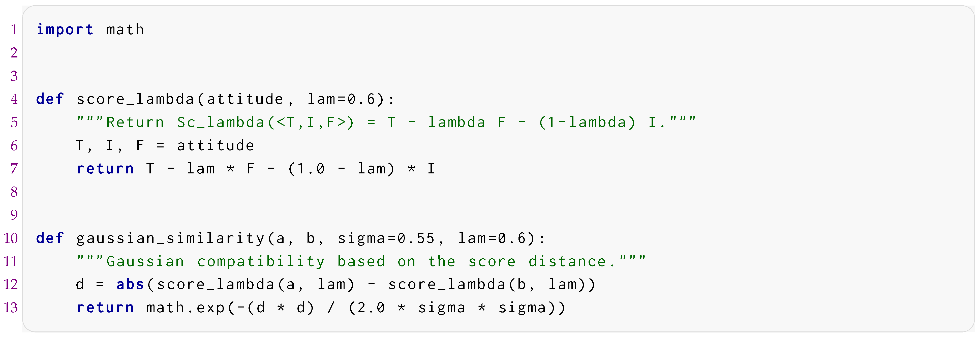
Listing 1: SVNS score and Gaussian similarity used by the Python implementation.
Listing shows the implementation of the candidate-selection distribution in Equation (A12). The Q-table does not appear in these candidate weights because Q-learning governs the preceding choice among keep, add, and delete; any factor depending only on would be common to all candidate targets and would cancel during normalization.
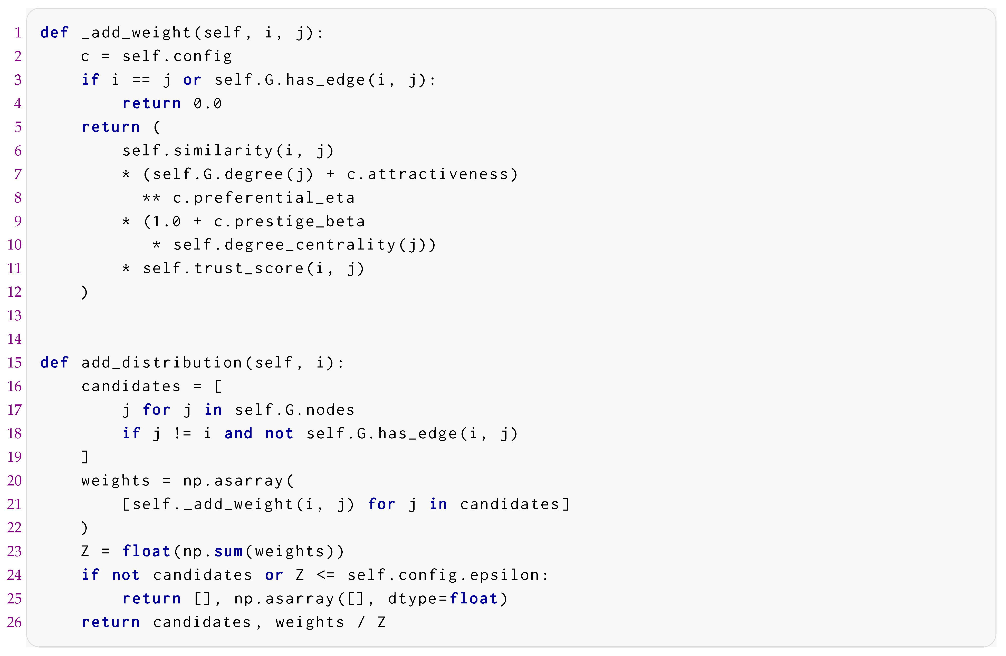
Listing 2: Candidate weights and normalized target selection for the add action in Equation (A12).
Listing illustrates the reproducible workflow used to compare the three topologies. Each run records the integration index, normalized cross-group reward index, score gap, clustering, path length, and integrator index.
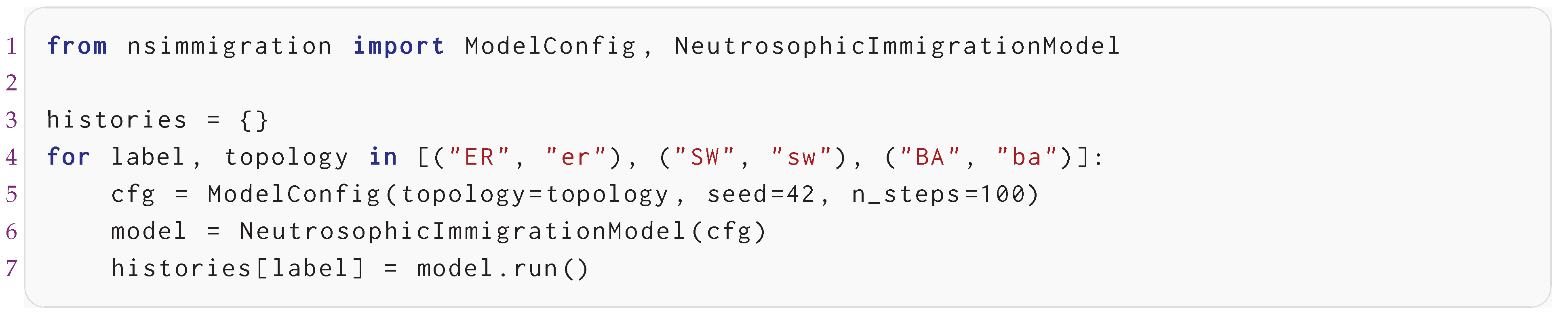
Listing 3: Minimal reproducible topology comparison.
8.2. Erd O s-R ényi Vs. Small-World Vs. Scale-Free
Figure 1 shows final network snapshots produced by the implementation of the three topologies [26]. Node colour represents the neutrosophic score and node size is proportional to degree, making hubs and potential cultural brokers visually apparent.
Figure 2 compares the integration index and the cross-group reward index under the three network families. The scale-free case is especially relevant because the presence of hubs can either accelerate integration or consolidate enclaves depending on the sign of cross-group reward and trust.
As summarized in Table 1, in this representative run, the small-world topology has the strongest local clustering, whereas the scale-free topology has the shortest effective paths. The scale-free case also attains the largest final values of both and , while the small-world case retains the strongest local closure. Thus, the three initial topologies remain distinguishable after adaptive rewiring: small-world integration depends more strongly on bridges between clustered neighbourhoods, whereas scale-free integration is more strongly mediated by hub-like brokers.
8.3. Simulation Results and Structural Analysis
Figure 3 tracks the mean value of the ten largest integrator indices. This quantity combines betweenness, cross-group exposure, and neutrosophic compatibility. It is more informative than degree alone because a high-degree agent inside a homogeneous enclave is not an integrator.
Figure 4 reports the final clustering coefficient and average path length. These structural indicators explain why topologies with similar may exhibit different levels of resilience. A clustered network can preserve local stability after a perturbation, but it may also preserve local segregation. A scale-free network, by contrast, may transmit perturbations more rapidly through hubs; this can be beneficial when hubs act as integrators and detrimental when they reinforce enclave structures.
More generally, the comparison suggests that network topology may affect not only the speed of convergence, but also the potential response of the system to external shocks. In an Erdos–Rényi network, shocks are expected to be dispersed across a relatively homogeneous random structure. In a small-world network, local clusters may absorb perturbations without immediately affecting the whole network, although the same clustering may also preserve segregated attitudes. In a scale-free network, the presence of hubs makes the system particularly sensitive to targeted interventions: supporting integrator hubs may accelerate convergence, whereas the loss or radicalization of a hub may rapidly reduce cross-group cohesion.
Table 2 reports the agents with the highest integrator index in the final scale-free network. The most relevant agents are not simply those with the highest score: they combine degree, cross-group exposure, betweenness, and closeness.
The table illustrates the analytical value of neutrosophic centrality. Agents with high cross-share and high closeness may be effective integrators even when their degree is moderate. Conversely, high-degree nodes must be evaluated through their cross-group reward and trust profile before they are interpreted as positive opinion leaders.
Figure 5 shows a migrant-fraction sensitivity scan in which the migrant fraction is varied over the grid while the small-world topology and all remaining parameters are held fixed. The same seed, 100, is used at every grid point so that changes are attributable as directly as possible to the migrant fraction rather than to a different random realization. The final integration index is compared with the host–migrant score gap. For illustration we set and ; a tipping warning requires simultaneously and .
For the illustrative thresholds used here, no grid point satisfies both warning conditions simultaneously, so this particular run does not identify a finite empirical on the scanned grid. This is preferable to forcing a threshold where the simulated evidence does not support one. The experiment instead demonstrates how a context-dependent threshold can be searched for once rewards, trust, initial attitudes, and policy parameters are calibrated. Collapse toward segregation is therefore not attributed to population share alone, but to the joint feedback among composition, attitudinal distance, trust, and adaptive link deletion.
9. Conclusions and Future Perspectives
This work strengthens the mathematical and methodological basis of a neutrosophic agent-based model for immigration and coexistence while preserving the SVNS framework . The model compares Erdos-Rényi, small-world, and scale-free topologies; introduces capacity-dependent utility; replaces myopic rewiring by Q-learning and DSmT-inspired trust aggregation; allows multiple migrant groups and asymmetric relational strength; and defines centrality-based integrator indices. Numerical simulations show how topology changes the interpretation of integration: small-world networks emphasize weak bridges between cohesive clusters, whereas scale-free networks emphasize the role of hubs. The neutrosophic representation also provides an additional interpretative advantage over scalar attitude models. A scalar model may register only a shift in mean attitude, whereas the triple distinguishes integration-oriented acceptance T, persistent rejection F, and indeterminacy I. In policy terms, this distinction is relevant because an intervention may not immediately convert rejection into acceptance; it may first increase indeterminacy, hesitation, or openness. The model can therefore represent an intermediate pre-integration phase that scalar models tend to hide. Finally, the migrant-fraction sensitivity scan provides a way to investigate when a demographic and attitudinal configuration becomes unstable and shifts toward enclave segregation. A further direction is the extension from SVNS attitudes to a refined four-component neutrosophic representation , in which indeterminacy I and neutrality N are represented as distinct components. This perspective is consistent with n-valued refined neutrosophic logic [30], quadripartitioned single-valued neutrosophic sets [9], and the explicit neutrosophic formulation [31]. In the present social setting, I could describe uncertainty, hesitation, or unresolved ambivalence, whereas N could represent a genuinely neutral or non-aligned attitude, distinct from both integration-oriented acceptance and segregation-oriented rejection.
Code availability
The Python implementation accompanying this article is provided as a reproducibility package [26] at
It contains the package nsimmigration, scripts for reproducing all figures, and a README with installation and execution instructions.
Acknowledgments
The research of G.N. has been carried out under the auspices of Gruppo Nazionale per le Strutture Algebriche, Geometriche e le loro Applicazioni (G.N.S.A.G.A.) of Istituto Nazionale di Alta Matematica (INdAM) “F. Severi”, Italy. C.F.M. thanks the Universities of Messina and Salerno and the Italian National Group for the Mathematical Physics (GNFM) of National Institute for Advanced Mathematics (INAM) “F. Severi”.
References
- Alam S.J., Geller A., Tsvetovat M. Networks in Agent-Based Social Simulation. In: Heppenstall A.J., Crooks A.T., See L.M., Batty M. (eds.), Agent-Based Models of Geographical Systems. Springer, 2012. doi: 10.1007/978-90-481-8927-4_11.
- Barabási A.-L., Albert R. Emergence of scaling in random networks. Science, vol. 286, no. 5439, pp. 509–512, 1999. doi: 10.1126/science.286.5439.509.
- Barrat A., Barthélemy M., Vespignani A. Dynamical Processes on Complex Networks. Cambridge University Press, 2008. doi: 10.1017/CBO9780511791383.
- Akram M. Single-Valued Neutrosophic Graphs. Singapore: Springer, 2018. doi: 10.1007/978-981-13-3522-8.
- Fathi S., ElGhawalby H., Salama A.A. On neutrosophic graph. Neutrosophic Knowledge, vol. 1, pp. 7–13, 2020.
- Benczik I.J., Benczik S.Z., Schmittmann B., Zia R.K.P. Opinion dynamics on an adaptive random network. Physical Review E, vol. 79, 046104, 2009. doi: 10.1103/PhysRevE.79.046104.
- Broumi S., Talea M., Bakali A., Smarandache F. Single valued neutrosophic graphs. Journal of New Theory, vol. 10, pp. 86–101, 2016.
- Chen Y., Hu Y., Huang S., et al. Social structure emergence: A multi-agent reinforcement learning framework. Proceedings of AAMAS, pp. 1807–1809, 2020.
- Chatterjee R., Majumdar P., Samanta S.K. On some similarity measures and entropy on quadripartitioned single valued neutrosophic sets. Journal of Intelligent & Fuzzy Systems, vol. 30, pp. 2475–2485, 2016. doi: 10.3233/IFS-152017.
- Chuang Y.-L., Chou T., D’Orsogna M.R. A network model of immigration: Enclave formation vs. cultural integration. Networks and Heterogeneous Media, vol. 14, no. 1, pp. 53–77, 2019. doi: 10.3934/nhm.2019004.
- Chuang Y.-L., Chou T., D’Orsogna M.R. A network model of immigration and coexistence. SIAM News, vol. 53, no. 3, 2020.
- Dezert J., Smarandache F. Fusion of imprecise, uncertain, and conflicting beliefs with DSm rules of combination. arXiv:math/0404305, 2004. https://arxiv.org/abs/math/0404305.
- Dezert J., Smarandache F. DSmT: A new paradigm shift for information fusion. arXiv:cs/0610175, 2006. https://arxiv.org/abs/cs/0610175.
- Freeman L.C. A set of measures of centrality based on betweenness. Sociometry, vol. 40, no. 1, pp. 35–41, 1977. doi: 10.2307/3033543.
- Gross T., Blasius B. Adaptive coevolutionary networks: a review. Journal of the Royal Society Interface, vol. 5, no. 20, pp. 259–271, 2008. doi: 10.1098/rsif.2007.1229.
- Haw D.J., Hogan S.J. A dynamical systems model of unorganized segregation. Journal of Mathematical Sociology, vol. 42, no. 3, pp. 113–127, 2018. doi: 10.1080/0022250X.2018.1427091.
- Holme P., Newman M.E.J. Nonequilibrium phase transition in the coevolution of networks and opinions. Physical Review E, vol. 74, 056108, 2006. doi: 10.1103/PhysRevE.74.056108.
- Hui Y., Dey A. A Study on Directed Neutrosophic Social Networks. IAENG International Journal of Applied Mathematics, vol. 50, no. 2, pp. 1–8, 2020.
- Kan U., Feng M., Porter M.A. An adaptive bounded-confidence model of opinion dynamics on networks. Journal of Complex Networks, vol. 11, no. 1, cnac055, 2023. doi: 10.1093/comnet/cnac055.
- Kozma B., Barrat A. Consensus formation on adaptive networks. Physical Review E, vol. 77, 016102, 2008. doi: 10.1103/PhysRevE.77.016102.
- Kandasamy W.B.V., Ilanthenral K., Smarandache F. Neutrosophic Graphs: A New Dimension to Graph Theory. EuropaNova ASBL, 2015.
- Kaviyarasu M., Aslam M., Afzal F., Saeed M.M., Mehmood A., Gul S. The connectivity indices concept of neutrosophic graph and their application of computer network, highway system and transport network flow. Scientific Reports, vol. 14, 4891, 2024. doi: 10.1038/s41598-024-54104-x.
- Mahapatra R., Samanta S., Pal M., Xin Q. Link prediction in social networks by neutrosophic graph. International Journal of Computational Intelligence Systems, vol. 13, no. 1, pp. 1699–1713, 2020. doi: 10.2991/ijcis.d.201015.002.
- Newman M.E.J. Networks: An Introduction. Oxford University Press, 2010. doi: 10.1093/acprof:oso/9780199206650.001.0001.
- Peng J., Tian C. A large-scale group decision-making method based on single-valued neutrosophic information under the social network environment. Journal of Systems Science and Mathematical Sciences, vol. 42, no. 4, pp. 935–954, 2022. doi: 10.12341/jssms21314.
- Nordo G., Munafò C.F., Martin N. neutrosophic-immigration-model: Python implementation of a neutrosophic agent-based network model for immigration and coexistence. GitHub repository, 2026. https://github.com/giorgionordo/neutrosophic-immigration-model. Accessed 16 August 2026.
- Schelling T.C. Models of segregation. American Economic Review, vol. 59, no. 2, pp. 488–493, 1969.
- Schelling T.C. Dynamic models of segregation. Journal of Mathematical Sociology, vol. 1, no. 2, pp. 143–186, 1971. doi: 10.1080/0022250X.1971.9989794.
- Smarandache F. A Unifying Field in Logics. Neutrosophy: Neutrosophic Probability, Set and Logic. Rehoboth: American Research Press, 1999.
- Smarandache F. n-valued refined neutrosophic logic and its applications to physics. Progress in Physics, vol. 4, pp. 143–146, 2013. Repository DOI: 10.6084/m9.figshare.1502593. Full text: https://fs.unm.edu/n-ValuedNeutrosophicLogic-PiP.pdf.
- Smarandache F. (T,I,N,F) neutrosophic set and logic (Truth, Indeterminacy, Neutrality, Falsehood). Critical Review, vol. XIV, pp. 20–28, 2017. https://fs.unm.edu/CR/TINF-NeutrosophicSetLogic.pdf.
- Smarandache F. The Score, Accuracy, and Certainty Functions determine a Total Order on the Set of Neutrosophic Triplets (T,I,F). Neutrosophic Sets and Systems, vol. 38, pp. 1–14, 2020. doi: 10.5281/zenodo.4300354.
- Sodenkamp M.A., Tavana M., Di Caprio D. An aggregation method for solving group multi-criteria decision-making problems with single-valued neutrosophic sets. Applied Soft Computing, vol. 71, pp. 715–727, 2018. doi: 10.1016/j.asoc.2018.07.020.
- Sutton R.S., Barto A.G. Reinforcement Learning: An Introduction. 2nd ed., MIT Press, 2018.
- Wang H., Smarandache F., Zhang Y.Q., Sunderraman R. Single Valued Neutrosophic Sets. Technical Sciences and Applied Mathematics, pp. 10–14, 2010.
- Wang F. Novel score function and standard coefficient-based single-valued neutrosophic MCDM for live streaming sales. Information Sciences, vol. 654, article 119836, 2024. doi: 10.1016/j.ins.2023.119836.
- Watkins C.J.C.H., Dayan P. Q-learning. Machine Learning, vol. 8, pp. 279–292, 1992. doi: 10.1007/BF00992698.
- Watts D.J., Strogatz S.H. Collective dynamics of small-world networks. Nature, vol. 393, pp. 440–442, 1998. doi: 10.1038/30918.
- Yang H.-L., Guo Z.-L., She Y., Liao X. On single valued neutrosophic relations. Journal of Intelligent & Fuzzy Systems, vol. 30, no. 2, pp. 1045–1056, 2016. doi: 10.3233/IFS-151827.
- Ye D., Zhang M., Sutanto D. Self-organization in an agent network: A mechanism and a potential application. Decision Support Systems, vol. 53, no. 3, pp. 406–417, 2012. doi: 10.1016/j.dss.2012.02.009.
- Ye J. Single-valued neutrosophic cross-entropy for multicriteria decision-making problems. Applied Mathematical Modelling, vol. 38, no. 3, pp. 1170–1175, 2014. doi: 10.1016/j.apm.2013.07.020.
Figure 1.
Final network snapshots generated by the companion implementation for ER, SW, and BA topologies. Node colour encodes and node size encodes degree.
Figure 1.
Final network snapshots generated by the companion implementation for ER, SW, and BA topologies. Node colour encodes and node size encodes degree.
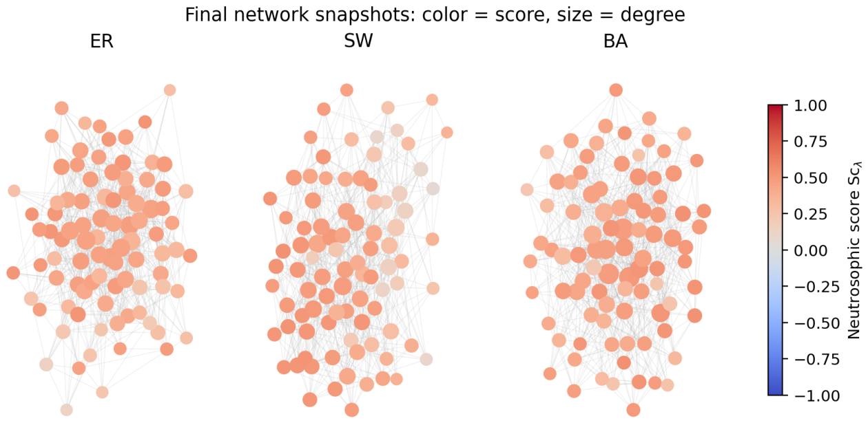
Figure 2.
Integration metrics for Erdos–Rényi (ER), small-world (SW), and Barabási–Albert-type scale-free (BA) topologies. Solid curves show ; dashed curves show .
Figure 2.
Integration metrics for Erdos–Rényi (ER), small-world (SW), and Barabási–Albert-type scale-free (BA) topologies. Solid curves show ; dashed curves show .
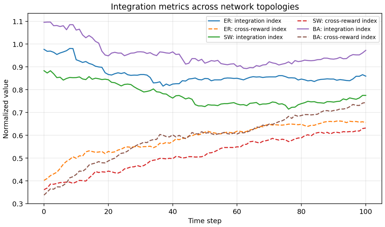
Figure 3.
Evolution of cultural-broker potential. The plotted quantity is the mean of the ten largest values of the integrator index .
Figure 3.
Evolution of cultural-broker potential. The plotted quantity is the mean of the ten largest values of the integrator index .
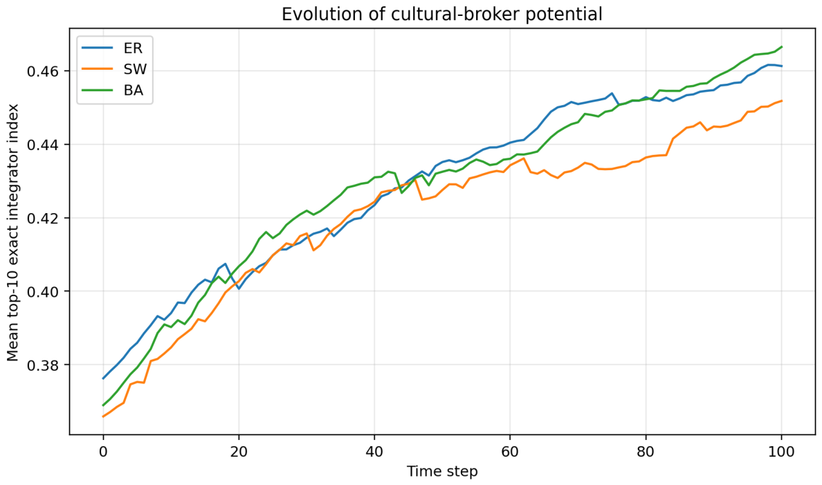
Figure 4.
Structural signatures of the final networks. Clustering measures local closure; average path length measures global reachability.
Figure 4.
Structural signatures of the final networks. Clustering measures local closure; average path length measures global reachability.
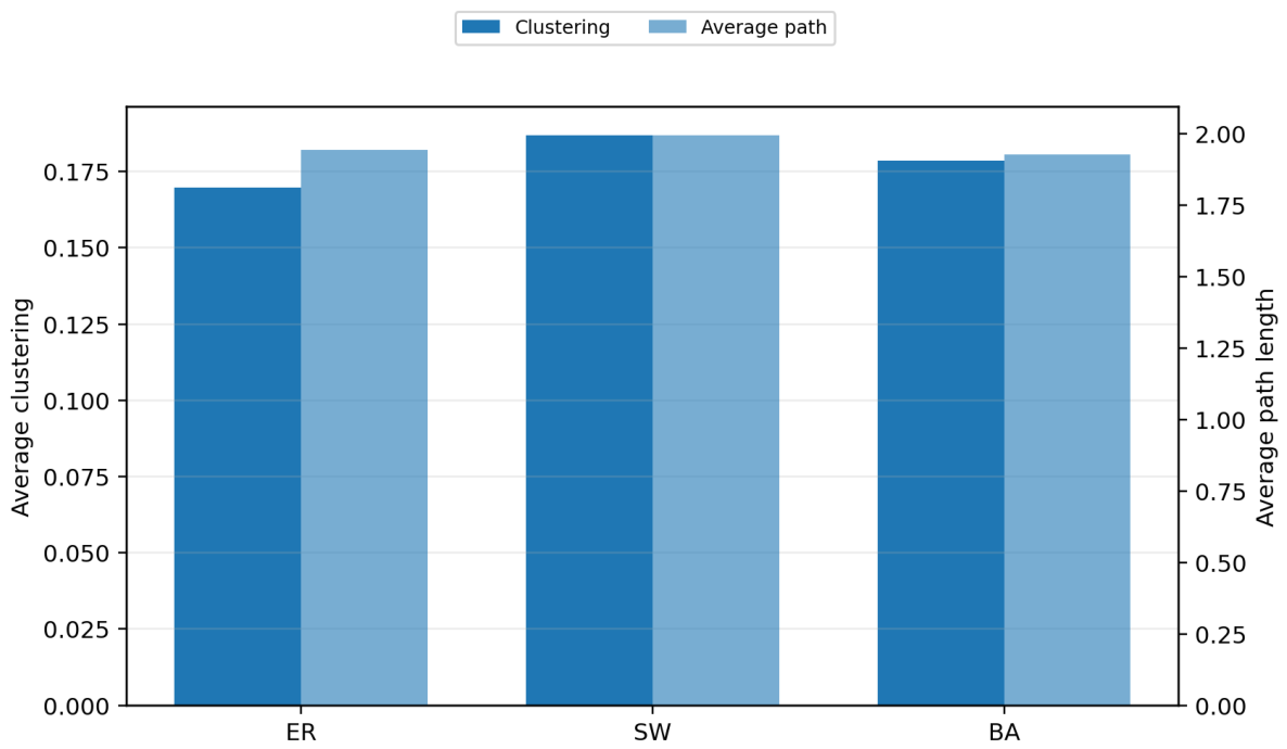
Figure 5.
Migrant-fraction sensitivity scan under small-world topology. The model records final integration and the final host–migrant score gap; horizontal lines show the illustrative warning levels and .
Figure 5.
Migrant-fraction sensitivity scan under small-world topology. The model records final integration and the final host–migrant score gap; horizontal lines show the illustrative warning levels and .
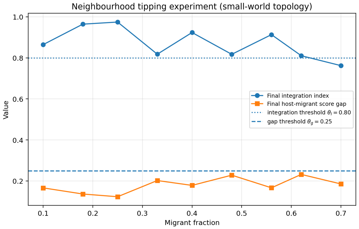

Table 1.
Final aggregate indicators in the three simulated scenarios. Average path length is computed on the largest connected component when the final graph is not connected.
Table 1.
Final aggregate indicators in the three simulated scenarios. Average path length is computed on the largest connected component when the final graph is not connected.
| Scenario | Integrator | Clustering | Avg. path | Score gap | ||
|---|---|---|---|---|---|---|
| ER | 0.859 | 0.656 | 0.461 | 0.170 | 1.944 | 0.176 |
| SW | 0.775 | 0.632 | 0.452 | 0.187 | 1.995 | 0.233 |
| BA | 0.973 | 0.744 | 0.466 | 0.178 | 1.929 | 0.149 |
Table 2.
Top cultural brokers in the final scale-free network.
| Node | Group | Degree | Score | NDC | NCC | Betweenness | Cross-share | |
|---|---|---|---|---|---|---|---|---|
| 53 | guest-2 | 21 | 0.389 | 0.179 | 0.556 | 0.025 | 0.952 | 0.499 |
| 32 | guest-1 | 11 | 0.358 | 0.096 | 0.503 | 0.007 | 1.000 | 0.481 |
| 23 | guest-2 | 10 | 0.402 | 0.084 | 0.491 | 0.004 | 1.000 | 0.480 |
| 60 | guest-2 | 13 | 0.371 | 0.113 | 0.511 | 0.008 | 0.923 | 0.466 |
| 47 | guest-2 | 22 | 0.371 | 0.195 | 0.558 | 0.026 | 0.818 | 0.465 |
| 49 | guest-2 | 18 | 0.399 | 0.157 | 0.546 | 0.014 | 0.833 | 0.460 |
| 46 | guest-1 | 11 | 0.407 | 0.091 | 0.484 | 0.004 | 0.909 | 0.455 |
| 62 | guest-1 | 10 | 0.408 | 0.091 | 0.487 | 0.005 | 0.900 | 0.454 |
Disclaimer/Publisher’s Note: The statements, opinions and data contained in all publications are solely those of the individual author(s) and contributor(s) and not of MDPI and/or the editor(s). MDPI and/or the editor(s) disclaim responsibility for any injury to people or property resulting from any ideas, methods, instructions or products referred to in the content. |
© 2026 by the authors. Licensee MDPI, Basel, Switzerland. This article is an open access article distributed under the terms and conditions of the Creative Commons Attribution (CC BY) license (http://creativecommons.org/licenses/by/4.0/).
Copyright: This open access article is published under a Creative Commons CC BY 4.0 license, which permit the free download, distribution, and reuse, provided that the author and preprint are cited in any reuse.