

Submitted:
26 August 2026
Posted:
27 August 2026
You are already at the latest version
Abstract
Continuous monitoring of permafrost dynamics remains challenging in remote high-mountain environments due to logistical constraints, harsh climatic conditions, and the limited availability of spatially distributed observations. In addition to direct temperature observations in boreholes, Autonomous Electrical Resistivity Tomography (A-ERT) offers significant potential for long-term monitoring by providing high temporal resolution observations of subsurface electrical properties, which is highly sensitive to freeze/thaw processes. This study presents the field validation of a low-power A-ERT system designed for long-term autonomous operation in extreme environments. The system was deployed at a high-altitude permafrost site near the Kumtor gold mine in the Central Tien Shan, Kyrgyzstan, representing the first application of continuous A-ERT monitoring in the Central Asian mountain ranges. The system operated continuously under harsh environmental conditions with air temperatures as low as −30 °C. Data quality remained consistently high throughout the monitoring period, with less than 1% of measurements removed during filtering, and inversion results with root-mean-square errors generally ranging between 3% and 4%. Time-lapse resistivity observations revealed strong seasonal freeze–thaw dynamics within the active layer and continued seasonal resistivity variations within the underlying permafrost despite permanently frozen conditions. Analysis of depth-dependent resistivity–temperature relationships revealed increasingly pronounced hysteresis behavior below the active layer, indicating that subsurface electrical properties were not controlled solely by temperature. This behavior likely reflects variations in unfrozen water content and pore connectivity within the fine-grained permafrost, where liquid water can persist at sub-zero temperatures. The results demonstrate the capability of the A-ERT system for reliable long-term autonomous monitoring in remote permafrost environments and investigation of coupled thermal and hydrological processes in permafrost systems.
Keywords:
autonomous electrical resistivity tomography (A‐ERT)
; permafrost monitoring
; freeze–thaw dynamics
; long‐term environmental monitoring
; temperature–resistivity hysteresis
; Central Tien Shan
Introduction
Permafrost in high-mountain environments plays a key role in regulating hydrological processes, controlling slope stability, and affecting infrastructure safety, particularly under ongoing climate change. In regions such as the Tien Shan Mountains, which are known as the “water tower of Central Asia”, these processes are of increasing concern due to warming trends (Chen et al., 2016, Marchenko et al., 2007) and the presence of critical infrastructure such as hydropower plants (De Keyser et al., 2026). However, despite increasing concern regarding permafrost degradation and its implications for hydrology, geomorphological hazards, and infrastructure stability, observational data in this region remain limited, especially when it comes to capturing both the spatial variability and temporal dynamics of the active layer and underlying permafrost (Mathys et al., 2025, 2026). Most existing monitoring efforts rely on borehole measurements (Marchenko, 2003; Marchenko et al., 2007; Zhao et al., 2010), which provide accurate but highly localized information and are often insufficient to resolve short-term variability or lateral heterogeneity.
Geophysical methods offer a valuable complement to these traditional approaches by providing spatially distributed information on subsurface conditions. Among these, Electrical Resistivity Tomography (ERT) has been widely used to investigate permafrost, as electrical resistivity is strongly influenced by the presence of ice and liquid water (Fortier et al., 1994; Herring et al., 2023; Kneisel et al., 2008). Numerous studies have demonstrated the applicability of ERT for mapping permafrost extent, estimating active layer thickness, and monitoring seasonal freeze–thaw processes (e.g., Hauck, 2002; Doetsch et al., 2015; Dafflon et al., 2016; Scandroglio et al., 2021). In particular, time-lapse ERT has proven effective for tracking temporal changes in subsurface conditions and identifying seasonal and interannual variability (e.g., Kneisel et al., 2014; Mollaret et al., 2019, Etzelmüller et al., 2020) and assessing unfrozen water content dynamics (Oldenborger and LeBlanc, 2018).
Recent developments in instrumentation have enabled automated and quasi-continuous ERT measurements, commonly referred to as Autonomous Electrical Resistivity Tomography (A-ERT). These systems significantly improve temporal resolution and allow the observation of rapid subsurface changes that are often not captured by conventional survey-based approaches (Hilbich et al., 2011; Keuschnig et al., 2017). A-ERT systems have been successfully applied in alpine (e.g., Hilbich et al., 2011), Arctic (e.g., Uhlemann et al., 2021; Cimpoiasu et al., 2025), and Antarctic environments (e.g., Farzamian et al., 2020, 2024a), demonstrating their capability for long-term monitoring of freeze–thaw dynamics under extreme environmental conditions. Nevertheless, autonomous long-term deployments remain relatively limited, and many studies still depend on manually repeated surveys, restricting temporal resolution and increasing logistical demands in remote environments (e.g., Buckel et al. 2023).
Despite recent advances, several methodological and technical challenges remain in the application of ERT and A-ERT to continuous permafrost monitoring. High contact resistance under frozen or dry conditions, together with reduced current penetration in highly resistive materials, can significantly affect data quality and system performance (Herring et al., 2023, Mollaret et al., 2019, Morard et al., 2024). In permafrost environments, subsurface resistivity commonly exceeds 10 kΩm and may even reach MΩm levels during winter when pore water freezes and conductive pathways become strongly reduced (e.g., Farzamian et al., 2024a) or when massive ice is encountered (Falatkova et al., 2019, Vonder Mühll et al., 2001, Wood et al., 2026). Under such conditions, resistivity systems must be capable of operating with very small injected currents while simultaneously maintaining sufficiently large voltage input ranges to remain within instrumental limits (e.g., Supper et al., 2014). In addition, systems intended for long-term deployment in remote mountain or polar environments must be robust, weather-resistant, low-power, and capable of autonomous operation with minimal field intervention.
Farzamian et al. (2024b) recently demonstrated the feasibility of long-term A-ERT monitoring in extreme environments using a low-cost, low-power, and robust monitoring solution. However, that study also identified several areas requiring further development, including improving system stability under high contact resistance conditions, enhancing data reliability and remote data transfer capabilities, and enabling adaptive acquisition strategies through remote system control. These challenges highlight the need for continued development of A-ERT systems specifically designed for harsh permafrost environments.
This study presents a year-round A-ERT dataset acquired from a high-altitude site near the Kumtor gold mine in the Central Tien Shan, Kyrgyzstan, located at approximately 3550m a.s.l. Although interest in permafrost monitoring in Central Asia has increased in recent years, the Tien Shan remains one of the least instrumented permafrost regions globally, with existing observations often limited to point measurements or short-term campaigns (Mathys et al., 2025). Introducing continuous and spatially distributed observations improves the understanding of permafrost dynamics and facilitates the validation of numerical models in the region. Building on previous system developments, this work evaluates the performance of an improved A-ERT system under harsh high-mountain conditions, with particular focus on system robustness, data quality, remote operation, and long-term autonomous monitoring. In addition, the study investigates the temporal evolution of subsurface resistivity and its relationship with temperature variations. By combining technological development with field-scale monitoring, this work provides both a technical assessment of A-ERT capabilities and new insights into subsurface freeze–thaw processes in a region where continuous geophysical observations remain scarce.
Study Area
The study site (Figure 1) is located on the Arabel plateau near the Kumtor gold mine in the Central Tien Shan, Kyrgyzstan, at an elevation of 3550 m a.s.l. The study site is characterized by a cold, semi-arid high-mountain climate and widespread mountain permafrost (Mathys et al., 2025). Mean annual air temperature is approximately −6.8 °C, while annual precipitation ranges between approximately 290 and 350 mm, with a substantial proportion falling as snow. The combination of high elevation, continental climatic conditions, and relatively low precipitation promotes the persistence of permafrost across large parts of the plateau environment. The A-ERT monitoring site is situated on a gentle slope composed predominantly of fine-grained sediments with sparse vegetation cover. In contrast to coarse blocky or rockwall mountain permafrost environments frequently investigated using geophysical methods (e.g., Hilbich et al., 2011; Abdulsamad et al., 2026), the Arabel plateau is characterized by silty to fine-grained materials with relatively high moisture retention capacity.
3. Material and Method
3.1. a-Ert System
The A-ERT system, referred to here as TRACE (Time-lapse Resistivity Assessment for Critical Environments), consists of a lightweight 4-point Light 10 W resistivity meter (Lippmann and Schwab Research Technology) and switch boxes enabling multi-electrode measurements, a solar-powered battery system, a two-way remote communication datalink (Schwab Research Technology), military-grade connectors, UAV- and temperature-rated cables, and a customized weather-resistant enclosure (IP67 and MIL-STD-810F rated) housing the main electronic components (Figure 2). The system was developed as a permanent monitoring installation for long-term autonomous operation under harsh high-mountain permafrost conditions.
TRACE is designed as a low-power monitoring system with an output current range between 1 μA and 100 mA. The minimum transmitter current of 1 μA is approximately one order of magnitude lower than the current resolution typically available in conventional commercial resistivity systems, making the system particularly suitable for monitoring the extremely high resistivities commonly encountered in frozen ground without overloading the receiver circuitry (Supper et al., 2014). The number of switch boxes is flexible and can be adapted according to the number of electrodes required for a specific monitoring configuration.
TRACE builds upon earlier A-ERT prototype systems described in detail in Farzamian et al. (2024b), while incorporating several hardware and operational improvements developed to address limitations identified during previous deployments in Antarctica and other extreme environments (Farzamian et al., 2024b). Earlier field experiments demonstrated the feasibility of low-cost and low-power A-ERT monitoring, but also highlighted challenges associated with high contact resistance, signal saturation, limited remote accessibility, and reduced measurement stability under highly resistive frozen conditions (Farzamian et al., 2024b). These limitations became particularly critical during winter periods when ground resistivity increased substantially as conductive pathways were reduced due to pore-water freezing.
To improve system performance under such conditions, several modifications were implemented in the current TRACE configuration. To mitigate errors associated with inadequate reference electrode contact, which become pronounced during periods of high contact resistance, the acquisition electronics were redesigned. In particular, 100 MΩ input resistors were introduced into the switch boxes to reduce dependence on grounding electrodes and improve measurement stability during potential measurements. In addition, the voltage input range was expanded to ±1 V to enable stable acquisition under the elevated voltage conditions expected in highly resistive environments. These modifications were specifically aimed at reducing signal saturation and improving data quality during winter monitoring periods. Additional protective electronic components were also incorporated to improve system resilience against lightning-related electrical disturbances, which are expected in exposed high-mountain environments.
The latest TRACE configuration also incorporates an upgraded remote communication architecture enabling real-time data transfer, remote monitoring of system status, and dynamic modification of acquisition parameters without requiring field access. This includes the ability to remotely adjust acquisition settings such as electrode configuration (e.g., Wenner, Dipole-Dipole or Schlumberger arrays), measurement frequency, current injection limits, stacking parameters, and survey timing in response to environmental conditions or power availability. These capabilities substantially improve operational flexibility and reduce the logistical constraints typically associated with long-term monitoring in remote permafrost regions. One important application of this functionality is the ability to increase acquisition frequency during freeze–thaw transition periods when subsurface conditions evolve rapidly.
3.2. Data Acquisition
The monitoring profile at the Kumtor site consists of 48 permanently installed stainless steel electrodes distributed along a 94 m profile, with 2m spacing, across fine-grained sediments, using the Wenner configuration. The permanent installation enabled repeated measurements using identical electrode geometry throughout the monitoring period, thereby minimizing geometric uncertainties between successive datasets and improving the consistency of time-lapse analysis. The system was configured for fully autonomous operation, allowing continuous acquisition of resistivity measurements throughout the seasonal freeze–thaw cycle.
The system was installed in October 2023 without the remote communication module, and data from the first monitoring campaign were downloaded manually during a subsequent site visit in late August 2024. In the present study, only data acquired during the first monitoring campaign (October 2023 to August 2024) are presented, providing an almost complete annual record for investigating seasonal active-layer and permafrost dynamics.
Ground temperature and meteorological data were obtained from the existing permafrost monitoring infrastructure installed at the site prior to the installation of the A-ERT system. Air temperature was measured at an automatic weather station, while ground temperatures were recorded in a borehole instrumented with temperature sensors at multiple depths down to 30 m (Hoelzle et al., 2025; Mathys et al., 2026). Both installations were located in the vicinity of the A-ERT profile, approximately 3–5 m from its midpoint. For the analyses presented in this study, temperatures at 0.5, 1, 2, 3, 5, and 10 m depth were used to investigate the relationship between subsurface thermal conditions and resistivity variations derived from the A-ERT monitoring system. All temperature and meteorological datasets were quality-controlled prior to analysis.
3.3. a-Ert Data Processing and Inversion
Due to the high temporal resolution of the autonomous monitoring setup and the large number of datasets generated during continuous operation, a semi-automated processing workflow was implemented following the general methodology proposed by Herring et al. (2023) and further developed for A-ERT applications by Farzamian et al. (2024a). The workflow was designed to efficiently process large time-series resistivity datasets while ensuring consistent quality control and minimizing subjective manual intervention. Such automated procedures are particularly important for long-term A-ERT deployments, where the number of repeated measurements can reach several hundreds or thousands of datasets per year, making manual inspection impractical.
The automated filtering workflow consisted of several sequential quality-control steps adapted from the workflow presented by Farzamian et al. (2024a). Measurements with negative apparent resistivities, stacking errors exceeding 10%, or extreme apparent resistivity values (>9 standard deviations from the dataset distribution) were removed. A moving-median filter was then applied in log-resistivity space, rejecting measurements deviating by more than 7% from the local median response. Electrodes associated with more than 30% rejected measurements were classified as faulty, and all measurements involving those electrodes were excluded. Compared to filtering approaches based solely on stacking error, the moving median filter is an effective additional step for identifying anomalous measurements (Rosset et al., 2013). This is because unrealistic spatial behavior can be still associated with stable stacking statistics (Tso et al., 2017). Finally, datasets with an excessive proportion of removed measurements (> 30%) were excluded entirely from inversion, as highly incomplete datasets may introduce instability and artifacts in time-lapse inversion results. Similar approaches have been shown to substantially improve inversion stability and consistency for automated permafrost monitoring datasets (e.g., Farzamian et al. 2024a).
3.4. a-Ert Data Inversion
Following filtering, all datasets were inverted using the open-source pyGIMLi framework (Rücker et al., 2017), incorporating the topography data (Günther et al., 2006). Similar to Farzamian et al. (2024a), an L1-norm (“blocky”) regularization scheme (Loke et al., 2003) was selected in order to better preserve sharp resistivity contrasts associated with the transition between thawed active-layer material and underlying frozen ground. Compared to smoothness-constrained inversion approaches, blocky regularization is generally more suitable for permafrost applications where abrupt boundaries with high resistivity contrast, i.e., between frozen and unfrozen zones, may exist (Farzamian et al., 2024a).
The inversion procedure employed a cascaded time-lapse approach, whereby each inverted model served as the starting model for the subsequent time step. This strategy improves temporal consistency between consecutive inversions and reduces inversion instability for large time-series datasets (Loke, 1999; Oldenborger et al., 2007). The initial model for the first dataset was defined as a homogeneous half-space using the average apparent resistivity of the corresponding survey. Data errors were estimated using a linear noise model consisting of a 4% relative error component and a small absolute error term (0.001 Ωm), values that are commonly adopted in ERT studies where detailed reciprocal-error analyses are unavailable (e.g., Herring et al., 2023). The inversion process was iterated until convergence criteria were satisfied, including acceptable data misfit levels or minimal changes in the objective function between iterations.
In addition to the analysis of apparent and inverted resistivity distributions, several complementary analyses were performed to investigate the relationship between electrical resistivity and subsurface thermal conditions. Resistivity evolution was examined both spatially and temporally through virtual borehole extraction, depth-dependent time-series analysis, and averaging within selected zones of interest. Virtual borehole analysis enabled direct comparison between inverted resistivity evolution and measured ground temperatures, facilitating assessment of freeze–thaw propagation with depth (e.g., Farzamian et al., 2024a).
Results and Discussion
4.1. System Performance and Data Quality Assessment
Figure 3 summarizes the operational performance of the TRACE system and the quality of the datasets acquired between October 2023 and August 2024, including the internal temperature of the resistivity meter, battery voltage, the number of filtered data points removed during processing, and the root-mean-square (RMS) error of the inverted models.
The internal temperature recorded within the system enclosure (Figure 3a) demonstrates that the monitoring system operated continuously under extreme seasonal conditions characteristic of the high-altitude permafrost environment. External air temperatures dropped below −30 °C during winter (cf. Figure 4a), while internal enclosure temperatures remained above -20 °C. The observed temperature offset likely reflects a combination of factors, including the insulating properties of the weather-resistant enclosure, heat dissipation from the electronic components, seasonal snow insulation during winter, and solar heating of the dark-colored housing during periods of high incoming radiation. Although internal temperatures remained below freezing for extended periods during winter, the system continued autonomous acquisition without operational interruption, indicating robust performance of both the electronic components and power-management system under prolonged sub-zero conditions.
Battery voltage evolution (Figure 3b) indicates stable long-term power supply throughout the monitoring period. Despite harsh winter conditions and reduced solar radiation during winter months, the solar-powered battery system was fully charged to support continuous autonomous operation. Battery voltage showed no large fluctuation thanks to the solar panel regulator and no evidence of power failure or critical discharge events were recorded. These results demonstrate the suitability of the low-power TRACE architecture for long-term deployment in remote environments with limited site accessibility.
The applied processing workflow resulted in only a small proportion of measurements being excluded from the final datasets (Figure 3c). Out of 360 measurements acquired per dataset, typically only 1–4 measurements were removed during filtering, corresponding to approximately 1% or less of the total acquired data. The low percentage of filtered measurements indicates a high overall data quality and generally low contact resistances throughout the year despite the challenging environmental conditions in frozen ground environments.
The RMS error of the inverted datasets remained relatively stable throughout the monitoring period, generally ranging between 3% and 4% (Figure 3d). These values indicate very good agreement between observed and modeled apparent resistivity data and confirm a good overall data quality. Slight seasonal variations in RMS error are likely associated with the higher resistivities and reduced signal-to-noise ratios characteristic of frozen conditions, as well as enhanced temporal variability during freeze–thaw transitions. Jumps in RMS error are likely a result of slight variations in the inversion process, where some datasets may reach convergence one iteration later or earlier than the previous time step, causing differences in RMS error values.
4.2. Seasonal Evolution of Apparent Resistivity and Temperature
Figure 4 presents the temporal evolution of air temperature (daily minimum, mean, and maximum), near-surface ground temperature at 0.5 m depth, and average apparent resistivity (ρa) for selected quadrupoles between October 2023 and August 2024. The figure also highlights periods with negative maximum daily air temperatures and illustrates the seasonal evolution of near-surface thermal and electrical conditions at the site.
Air temperature exhibited large variability during the monitoring period, ranging from −33.9 to 18.9 °C. Near-surface ground temperature showed damped variations compared to atmospheric conditions, ranging from −8.5 to 6.3 °C, with negligible daily fluctuations.
Average ρa displayed a pronounced seasonal cycle across all investigated electrode spacings (Figure 4c). In general, resistivity increased progressively during autumn and winter as ground temperatures decreased and conductive pore-water pathways became increasingly restricted by freezing. Maximum resistivity values were observed during late winter and early spring, followed by a rapid decrease during thawing conditions in spring and early summer. This overall pattern demonstrates the strong sensitivity of electrical resistivity to seasonal freeze–thaw dynamics.
The magnitude and variability of resistivity differed substantially with electrode spacing. The shallowest measurements, corresponding to the 2 m electrode spacing (~ 1m depth of investigation), exhibited the largest temporal variability, with apparent resistivity values ranging from 86 to 785 Ωm. In contrast, larger electrode spacings, which sample deeper subsurface regions, showed progressively higher mean resistivity values with reduced seasonal variability, demonstrating that shallow subsurface layers are more strongly influenced by seasonal freeze–thaw processes, whereas deeper permafrost layers remain thermally buffered and comparatively stable throughout the year. Shallow apparent resistivity values reached maximum levels during mid- to late March, whereas deeper spacings continued increasing until April, reflecting the expected delayed propagation of freezing conditions with depth.
During the sustained freezing period in late October 2023, near-surface ground temperatures remained close to the thawing point for an extended period while shallow resistivity constantly increased, indicating the presence of zero-curtain conditions associated with progressive freezing of pore ice.
Several short-term resistivity fluctuations were observed during transitional periods, particularly in spring. Temporary decreases in shallow apparent resistivity coincided with short-lived warming events with maximum daily air temperatures near or > 0 °C, despite near-surface ground temperatures remaining predominantly below 0 °C (e.g., during late March 2024). These observations suggest that electrical resistivity is highly sensitive to transient changes in unfrozen water content and moisture connectivity within the active layer. These findings are also in agreement with other studies in different environments of Antarctica (e.g., Farzamian et al., 2024a; 2024b), demonstrating the potential of A-ERT in studying the impact of short-lived meteorological events on active layer and permafrost dynamics.
4.3. Seasonal Evolution of 2d Inverted Resistivity Models
Selected inverted 2D resistivity models illustrating the seasonal evolution of subsurface electrical resistivity between October 2023 and August 2024 are presented in Figure 5. The selected models represent key stages of the annual freeze–thaw cycle and provide a spatial overview of temporal resistivity variations within the active layer and underlying permafrost.
Figure 5a shows the first A-ERT survey acquired in late October 2023 and serves as the reference model at the beginning of the monitoring period. At this stage, near-surface freezing had already started, although shallow resistivity values remained comparatively low. Figure 5b shows the model from mid-January 2024, representing winter conditions when ground temperatures within the active layer had decreased substantially below 0 °C and apparent resistivity values began increasing in the shallow subsurface. The third model (Figure 5c), corresponding to mid-April 2024, represents the late winter to early spring transition period during which the highest resistivity values were observed, particularly within deeper portions of the profile. This timing corresponds well with the maximum apparent resistivity values observed in the temporal analysis (Figure 4c). In contrast, the fourth and fifth examples (Figure 5d and Figure 5e), representing early May 2024 and mid-August 2024, illustrate the onset of thawing conditions and late summer conditions, respectively. The early May model coincides with the zero-curtain period and resistivity decrease within the active layer, while the August model reflects maximum seasonal thaw depth and minimum shallow resistivity values.
The inverted models reveal a relatively conductive near-surface zone within approximately the upper 2 m of the subsurface, consistent with the maximum active-layer thickness of 1.8 m reported for the site (Mathys et al., 2025). This shallow zone exhibits large temporal variability throughout the monitoring period, indicating strong sensitivity to seasonal freeze–thaw dynamics and associated changes in liquid water content, as also observed in shallow ρa data (cf. Figure 4c). Below the active layer, corresponding to the underlying permafrost, resistivity variations become progressively smaller with depth, reflecting the attenuation of seasonal thermal fluctuations. Nevertheless, clear seasonal evolution remains visible within the upper permafrost zone, particularly between approximately 2 and 10 m depth. Resistivity increases during winter and early spring indicate continued cooling and gradual reduction of unfrozen water content even under permanently frozen conditions. At greater depths below approximately 10 m, resistivity variability becomes comparatively limited, suggesting thermally stable permafrost conditions with minimal seasonal influence.
One notable feature of the models is the conductive behavior of the shallow subsurface during winter conditions. Compared with the coarse-grained permafrost environments, where freezing often produces very sharp resistivity increases of the active layer (e.g., Farzamian et al., 2024 a, b), the active layer at the Kumtor site remains comparatively conductive throughout much of the winter period. This behavior likely reflects both the fine-grained nature of the sediments and the occurrence of short-lived warming events during winter and spring, as seen in Figure 4. Fine-grained soils are capable of retaining substantial amounts of unfrozen water below 0 °C due to capillary and adsorptive effects, thereby maintaining electrically conductive pathways even under frozen conditions (Williams, 1964). As a result, resistivity evolution appears more gradual and less abrupt than typically observed in e.g., the more coarse-grained substrates in the European Alps (cf. Hilbich et al. 2011, Morard et al. 2024).
In addition, the minimum electrode spacing of 2 m limits the sensitivity of the system to very shallow near-surface processes, and shallow freezing within the uppermost decimeters may therefore be only partially resolved in the inverted models. The models also reveal lateral variability along the profile, with stronger temporal dynamics observed particularly in the left portion of the section. This spatial heterogeneity likely reflects local variations in soil properties, or moisture distribution, and variations in ground ice content, which was also indicated by refraction seismic data and ice content modelling in Mathys et al. (2025).
4.4. Depth-Dependent Temperature–Resistivity Relationships and Hysteresis
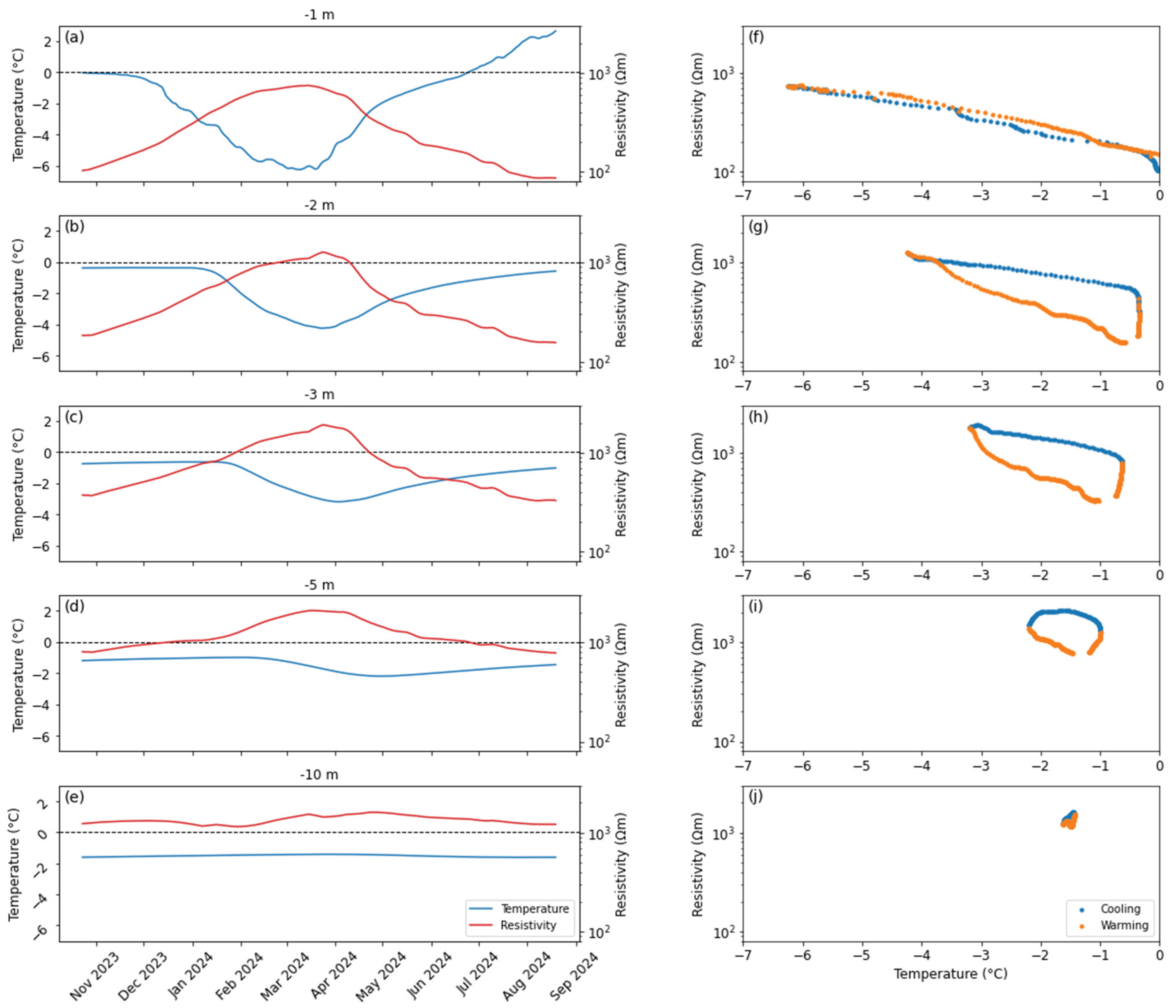
Figure 6 presents the temporal evolution of ground temperature and extracted resistivity values at the virtual borehole (located at the midpoint of the A-ERT profile, close to the borehole) together with the corresponding temperature–resistivity relationships during cooling and warming periods. The combined analysis reveals clear depth-dependent differences in the thermal–electrical response of the subsurface and demonstrates the progressive development of hysteresis below the active layer.
At 1 m depth (Figure 6 a, f), corresponding to the active layer, temperature exhibited the largest seasonal variability, ranging from −6.3 to 2.7 °C with a standard deviation of 2.6 °C. Resistivity varied between approximately 86 and 744 Ωm (standard deviation 221 Ωm) and reached its maximum values (>700 Ωm) during mid-March, coinciding with the minimum ground temperatures (<−6 °C). The resistivity evolution closely followed the seasonal thermal cycle, increasing during autumn and winter as temperatures decreased and declining rapidly during spring thawing. The relatively synchronous behavior of temperature and resistivity, together with the limited separation between the cooling and warming trajectories, indicates that electrical properties at this depth are primarily controlled by seasonal freezing and thawing processes affecting liquid water content and pore connectivity within the active layer.
One notable feature is the apparent autumn zero-curtain period observed between late October and mid-November 2023, during which ground temperature remained close to the freezing point while resistivity continued to increase gradually, suggesting that phase-change processes were still ongoing despite limited temperature variations. However, the onset of freezing was not fully captured because monitoring began in late October 2023, after part of the autumn freeze-up period had already occurred. In contrast, only a weak zero-curtain signature was observed during spring thawing, when both temperature and resistivity transitioned relatively rapidly from winter to summer conditions. This behavior differs from observations at Antarctic monitoring sites reported by Farzamian et al. (2024a, b), where the thawing-season zero-curtain was more prolonged than the freezing-season zero-curtain. Although snow-cover observations are not available for the Kumtor site, differences in snow accumulation and its insulating effect may partly explain these contrasting seasonal responses.
At 2 and 3 m depth (Figure 6b, c, g, h), temperatures remained entirely below 0 °C throughout the monitoring period, ranging from approximately −4.2 to −0.3 °C at 2 m and from −3.2 to −0.6 °C at 3 m. Despite these comparatively small thermal variations, resistivity exhibited pronounced seasonal changes, reaching maximum values of approximately 1280 Ωm and 1910 Ωm, respectively, with standard deviations exceeding 340 Ωm and 460 Ωm. Although the timing of maximum resistivity generally coincided with the lowest ground temperatures, the seasonal response became progressively delayed relative to the active layer. The corresponding temperature–resistivity plots reveal a clear separation between cooling and warming trajectories, demonstrating that, for the same temperature, resistivity depends on the thermal history of the ground. This behavior suggests that below the active layer, electrical properties are no longer controlled solely by temperature, but are also influenced by gradual changes in unfrozen water content, pore-scale connectivity, and ice distribution within the fine-grained permafrost.
At 5 m depth (Figure 6 d, i), temperature variability was strongly attenuated, remaining between approximately −2.2 and −1.0 °C (standard deviation 0.42 °C), whereas resistivity continued to vary substantially between approximately 780 and 2100 Ωm (standard deviation >400 Ωm). Furthermore, the resistivity maximum occurred earlier than the temperature minimum, indicating an increasing decoupling between thermal and electrical responses. The hysteresis loop also became more pronounced despite the relatively narrow temperature range, suggesting that seasonal changes in unfrozen water distribution and pore connectivity continue to influence the electrical properties of the permafrost. However, reduced inversion sensitivity at depth associated with the strong resistivity contrast between the active layer and the underlying permafrost may also contribute to the observed behavior and should therefore be considered when interpreting these results.
At 10 m depth (Figure 6 e, j), temperature remained nearly constant throughout the monitoring period, varying only between −1.62 and −1.43 °C with a standard deviation of 0.07 °C. Resistivity variability was also substantially reduced compared with shallower layers, and only minor hysteresis was observed. These results indicate a thermally stable permafrost zone with limited seasonal influence, although the reduced sensitivity of the inverted models at this depth may further suppress the apparent electrical variability.
Overall, the results demonstrate a progressive transition from direct thermal control of resistivity within the active layer to increasingly complex thermo-hydrological controls within the underlying permafrost. The observed hysteresis is consistent with previous studies of fine-grained permafrost. For example, Tomaškovičová and Ingeman-Nielsen (2023) reported that, for the same sub-zero temperature, resistivity during freezing is generally higher than during thawing because ice formation progressively disconnects conductive pore-water pathways, whereas thawing reconnects these pathways before complete melting occurs. Consequently, the relationship between resistivity and temperature is not unique but depends on the thermal history of the ground. Similar processes may explain the hysteresis observed at the Kumtor site, although its magnitude appears less pronounced than that reported for Greenland permafrost. These findings further suggest that the use of a single petrophysical relationship to estimate unfrozen water content from resistivity measurements may introduce systematic errors and that separate calibrations for freezing and thawing conditions may be required (Tomaškovičová, 2018). Nevertheless, additional laboratory measurements and site-specific petrophysical investigations are needed to distinguish the relative contributions of unfrozen water dynamics and inversion uncertainty to the observed hysteresis.
Conclusions
This study presented the development and field validation of the TRACE A-ERT system for continuous subsurface monitoring under harsh high-mountain permafrost conditions in the Central Tien Shan, Kyrgyzstan. Throughout the monitoring period, the system maintained stable autonomous operation with no interruptions or operational failures. The results demonstrate that the system is capable of reliable long-term autonomous operation in remote environments characterized by extreme temperatures, limited accessibility, and strong seasonal freeze–thaw variability.
The acquired datasets revealed clear seasonal evolution of subsurface resistivity associated with freeze–thaw dynamics within the active layer and upper permafrost. Shallow subsurface resistivity exhibited strong seasonal variability and responded rapidly to atmospheric forcing, whereas deeper layers showed delayed and smoother responses reflecting attenuation of thermal signals with depth.
An important outcome of this study is the observation that resistivity evolution within the permafrost layer was not controlled solely by temperature. Despite permanently frozen conditions below the active layer, significant seasonal resistivity variations and pronounced temperature–resistivity hysteresis behavior were observed. These findings suggest that unfrozen water dynamics, pore-scale connectivity, and freeze–thaw history exert a strong influence on subsurface electrical properties within the fine-grained sediments of the Kumtor site.
Beyond the specific permafrost application presented here, the TRACE system demonstrates broader potential for long-term autonomous geophysical monitoring in remote and environmentally challenging settings. The combination of low-power operation, remote communication capabilities, adaptive acquisition control, and robust field performance makes the system suitable for a wide range of environmental, hydrological, cryospheric, and infrastructure monitoring applications where continuous subsurface observations are required. In parallel, the future development of a web-based platform for processing and inversion of A-ERT data may enable near real-time subsurface imaging and interpretation. Such an integrated monitoring framework opens possibilities for autonomous early-warning systems, continuous assessment of subsurface dynamics, and scalable deployment of geophysical observatories in remote environments.
Author Contributions
Conceptualization, M.F., C.Ha., and C.Hi.; methodology, M.F., T.H., M.E., E.L., and A.S.; software, M.F., T.H., and A.S.; validation, M.F., M.E., and T.H.; formal analysis, M.F., and T.M.; investigation, M.F., A.Z., C.Hi., T.M., and M.H.; resources, M.F., C.Ha., C.Hi., M.H, and T.M.; writing—original draft preparation, M.F; writing—review and editing, all authors; visualization, M.F., and T.M.; supervision, M.F., C.Ha., and M.H; project administration, C.Hi., C.Ha., and M.H.; funding acquisition, C.Ha. All authors have read and agreed to the published version of the manuscript.
Funding
This research received support from a technology grant received from the Swiss Polar Institute (SPI Technogrant TEG-2021-003: ERT-PERM) and the project Cryospheric Observation and Modelling for Improved Adaptation in Central Asia (CROMO-ADAPT) (contract no. 81072443), funded by the Swiss Agency for Development and Cooperation.
Acknowledgments
The authors gratefully acknowledge the University of Fribourg for its financial and logistical support of this research. We sincerely thank all colleagues and field assistants whose dedication and hard work made the successful installation and maintenance of the monitoring system possible under challenging high-mountain conditions. We also express our sincere appreciation to our local partners, particularly the Central Asian Institute for Applied Geosciences (CAIAG), Kyrgyzstan, for their collaboration, technical support, and assistance throughout the field campaigns.
Conflicts of Interest
The authors declare that they have no known competing financial interests or personal relationships that could have appeared to influence the work reported in this paper.
References
- Buckel, J.; Mudler, J.; Gardeweg, R.; Hauck, C.; Hilbich, C.; Frauenfelder, R.; Kneisel, C.; Buchelt, S.; Blöthe, J. H.; Hördt, A.; Bücker, M. Identifying mountain permafrost degradation by repeating historical electrical resistivity tomography (ERT) measurements. The Cryosphere 2023, 17, 2919–2940. [Google Scholar] [CrossRef]
- Chen, Y.; Li, W.; Deng, H.; Fang, G.; Li, Z. Changes in Central Asia’s Water Tower: Past, Present and Future. Scientific Reports 2016, 6, 35458. [Google Scholar] [CrossRef] [PubMed]
- Cimpoiasu, M. O.; Kuras, O.; Harrison, H.; Wilkinson, P. B.; Meldrum, P.; Chambers, J. E.; Liljestrand, D.; Oroza, C.; Schmidt, S. K.; Sommers, P.; Vimercati, L.; Irons, T. P.; Lyu, Z.; Solon, A.; Bradley, J. A. High-resolution 4D electrical resistivity tomography and below-ground point sensor monitoring of High Arctic deglaciated sediments capture zero-curtain effects, freeze–thaw transitions, and mid-winter thawing. The Cryosphere 2025, 19, 401–421. [Google Scholar] [CrossRef]
- De Keyser, J.; Osuna, P.; Hayes, D. S.; Habersack, H. A review of hydropower in Central Asia: Past, present, and future. Renewable and Sustainable Energy Reviews 2026, 226. [Google Scholar] [CrossRef]
- Doetsch, J.; Ingeman-Nielsen, T.; Christiansen, A. V.; Fiandaca, G.; Auken, E.; Elberling, B. Direct current (DC) resistivity and induced polarization (IP) monitoring of active layer dynamics at high temporal resolution. Cold Regions Science and Technology 2015, 119, 16–28. [Google Scholar] [CrossRef]
- Etzelmüller, B.; Guglielmin, M.; Hauck, C.; Hilbich, C.; Hoelzle, M.; Isaksen, K.; Noetzli, J.; Oliva, M.; Ramos, M. Twenty years of European mountain permafrost dynamics – the PACE legacy. Environmental Research Letters 2020, 15(10), 104070. [Google Scholar] [CrossRef]
- Falatkova, K.; Šobr, M.; Neureiter, A.; Schöner, W.; Janský, B.; Häusler, H.; Engel, Z.; Bene, V. Development of proglacial lakes and evaluation of related outburst susceptibility at the Adygine ice-debris complex, northern Tien Shan. Earth Surface Dynamics 2019, 7(1), 301–320. [Google Scholar] [CrossRef]
- Farzamian, M.; Vieira, G.; Monteiro Santos, F. A.; Yaghoobi Tabar, B.; Hauck, C.; Paz, M. C.; Bernardo, I.; Ramos, M.; de Pablo, M. A. Detailed detection of active layer freeze–thaw dynamics using quasi-continuous electrical resistivity tomography (Deception Island, Antarctica). The Cryosphere 2020, 14, 1105–1120. [Google Scholar] [CrossRef]
- Farzamian, M.; Herring, T.; Vieira, G.; de Pablo, M. A.; Yaghoobi Tabar, B.; Hauck, C. Employing automated electrical resistivity tomography for detecting short- and long-term changes in permafrost and active layer dynamics in the Maritime Antarctic. The Cryosphere 2024a, 18, 4197–4213. [Google Scholar] [CrossRef]
- Farzamian, M.; Blanchy, G.; McLachlan, P.; Vieira, G.; Esteves, M.; de Pablo, M. A.; Triantafilis, J.; Lippmann, E.; Hauck, C. Advancing permafrost monitoring with Autonomous Electrical Resistivity Tomography (A-ERT): Low-cost instrumentation and open-source data processing tool. Geophysical Research Letters 2024b, 51, e2023GL105770. [Google Scholar] [CrossRef]
- Fortier, R.; Allard, M.; Seguin, M. K. Effect of physical properties of frozen ground on electrical resistivity logging. Cold Regions Science and Technology 1994, 22(4), 361–384. [Google Scholar] [CrossRef]
- Günther, T.; Rücker, C.; Spitzer, K. Three-dimensional modelling and inversion of DC resistivity data incorporating topography – II. Inversion. Geophysical Journal International 2006, 166(2), 506–517. [Google Scholar] [CrossRef]
- Hauck, C. Frozen ground monitoring using DC resistivity tomography. Geophysical Research Letters 2002, 29(21). [Google Scholar] [CrossRef]
- Hauck, C.; Vonder Mühll, D.; Maurer, H. Using DC resistivity tomography to detect and characterize mountain permafrost. Geophysical Prospecting 2003, 51(4), 273–284. [Google Scholar] [CrossRef]
- Herring, T.; Lewkowicz, A. G.; Hauck, C.; Hilbich, C.; Mollaret, C.; Oldenborger, G. A.; Uhlemann, S.; Calmels, F.; Farzamian, M.; Scandroglio, R. Best practices for using electrical resistivity tomography to investigate permafrost. Permafrost and Periglacial Processes 2023, 34(4), 494–512. [Google Scholar] [CrossRef]
- Hilbich, C.; Fuss, C.; Hauck, C. Automated time-lapse ERT for improved process analysis and monitoring of frozen ground. Permafrost and Periglacial Processes 2011, 22(4), 306–319. [Google Scholar] [CrossRef]
- Hilbich, C.; Hauck, C.; Hoelzle, M.; Scherler, M.; Schudel, L.; Völksch, I.; Mäusbacher, R.; Mäusbacher, R. Monitoring mountain permafrost evolution using electrical resistivity tomography: A 7-year study of seasonal, annual, and long-term variations at Schilthorn, Swiss Alps. Journal of Geophysical Research: Earth Surface 2008, 113, F01S90. [Google Scholar] [CrossRef]
- Hoelzle, M. and the CROMO-Adapt Project Permafrost boreholes and geophysical observations in Central Asia; EGU General Assembly 2025, 2025; p. EGU25-7199. [Google Scholar] [CrossRef]
- Keuschnig, M.; Krautblatter, M.; Hartmeyer, I.; Fuss, C.; Schrott, L. Automated electrical resistivity tomography testing for early warning in unstable permafrost rock walls around Alpine infrastructure. Permafrost and Periglacial Processes 2017, 28(1), 158–171. [Google Scholar] [CrossRef]
- Kneisel, C.; Hauck, C.; Fortier, R.; Moorman, B. Advances in geophysical methods for permafrost investigations. Permafrost and Periglacial Processes 2008, 19, 157–178. [Google Scholar] [CrossRef]
- Kneisel, C.; Rödder, T.; Schwindt, D. Frozen ground dynamics resolved by multi-year and year-round electrical resistivity monitoring at three alpine sites in the Swiss Alps. Near Surface Geophysics 2014, 12, 117–132. [Google Scholar] [CrossRef]
- Loke, M. H. Time-Lapse Resistivity Imaging Inversion. In Proceedings of the 5th EEGS-ES Meeting; 1999. [Google Scholar] [CrossRef]
- Loke, M. H.; Acworth, I.; Dahlin, T. A comparison of smooth and blocky inversion methods in 2D electrical imaging surveys. Exploration Geophysics 2003, 34(3), 182–187. [Google Scholar] [CrossRef]
- Mathys, T.; Azimshoev, M.; Bektursunov, Z.; Hauck, C.; Hilbich, C.; Duishonakunov, M.; Kayumov, A.; Kassatkin, N.; Kapitsa, V.; Martin, L. C. P.; Mollaret, C.; Navruzshoev, H.; Pohl, E.; Saks, T.; Silmonov, I.; Musaev, T.; Usubaliev, R.; Hoelzle, M. Quantifying permafrost ground ice contents in the Tien Shan and Pamir (Central Asia): a petrophysical joint inversion approach using a geometric mean model. The Cryosphere 2025, 19, 6591–6628. [Google Scholar] [CrossRef]
- Mathys, T.; Marchenko, S. S.; Westermann, S.; Gregor, L.; Martin, L. C. P.; Duishonakunov, M.; Hauck, C.; Farzamian, M.; Herring, T.; Hilbich, C.; Kenzhebaev, R.; Esenaman uulu, M.; Musaev, T.; Bektursunov, Z.; Usubaliev, R.; Brining, I.; Saks, T.; Hoelzle, M. Mapping permafrost distribution and thaw depths in the Inner Tien Shan: A CryoGrid-based modeling approach integrating geophysical data; EGUsphere, 2026. [Google Scholar] [CrossRef]
- Marchenko, S. S. Borehole and active-layer monitoring in the northen Tien Shan (Kazakhstan). In Proceedings of the 8th International Conference on Permafrost; 2003. [Google Scholar]
- Marchenko, S. S.; Gorbunov, A. P.; Romanovsky, V. E. Permafrost warming in the Tien Shan Mountains, Central Asia. Global and Planetary Change 2007, 56, 311–327. [Google Scholar] [CrossRef]
- Mollaret, C.; Hilbich, C.; Pellet, C.; Flores-Orozco, A.; Delaloye, R.; Hauck, C. Mountain permafrost degradation documented through a network of permanent electrical resistivity tomography sites. The Cryosphere 2019, 13, 2557–2578. [Google Scholar] [CrossRef]
- Morard, S.; Hilbich, C.; Mollaret, C.; Pellet, C.; Hauck, C. 20-year permafrost evolution documented through petrophysical joint inversion, thermal and soil moisture data. Environmental Research Letters 2024, 19, 074074. [Google Scholar] [CrossRef]
- Oldenborger, G. A.; Knoll, M. D.; Routh, P. S.; LaBrecque, D. J. Time-lapse ERT monitoring of an injection/withdrawal experiment in a shallow unconfined aquifer. Geophysics 2007, 72(4). [Google Scholar] [CrossRef]
- Oldenborger, G. A.; LeBlanc, A. M. Monitoring changes in unfrozen water content with electrical resistivity surveys in cold continuous permafrost. Geophysical Journal International 2018, 215(2), 965–977. [Google Scholar] [CrossRef]
- Rosset, E.; Hilbich, C.; Schneider, S.; Hauck, C. Automatic filtering of ERT monitoring data in mountain permafrost. Near Surface Geophysics 2013, 11(4), 423–433. [Google Scholar] [CrossRef]
- Rücker, C.; Günther, T.; Wagner, F. M. pyGIMLi: An open-source library for modelling and inversion in geophysics. Computers & Geosciences 2017, 109, 106–123. [Google Scholar] [CrossRef]
- Scandroglio, R.; Draebing, D.; Offer, M.; Krautblatter, M. 4D quantification of alpine permafrost degradation in steep rock walls using a laboratory-calibrated electrical resistivity tomography approach. Near Surface Geophysics 2021, 19(2), 241–260. [Google Scholar] [CrossRef]
- Supper, R.; Ottowitz, D.; Jochum, B.; Römer, A.; Pfeiler, S.; Kauer, S.; Keuschnig, M.; Ita, A. Geoelectrical monitoring of frozen ground and permafrost in alpine areas: Field studies and considerations towards an improved measuring technology. Near Surface Geophysics 2014, 12(1), 93–115. [Google Scholar] [CrossRef]
- Tso, C. H. M.; Kuras, O.; Wilkinson, P. B.; Uhlemann, S.; Chambers, J. E.; Meldrum, P. I.; Binley, A.; Graham, J. Improved characterisation and modelling of measurement errors in electrical resistivity tomography (ERT) surveys. Journal of Applied Geophysics 2017, 146, 103–119. [Google Scholar] [CrossRef]
- Tomaškovičová, S. Coupled thermo-geophysical inversion for permafrost monitoring. PhD thesis, Department of Civil Engineering, Technical University of Denmark, 2018. Available online: https://backend.orbit.dtu.dk/ws/files/145164684.
- Tomaškovičová, S.; Ingeman-Nielsen, T. Quantification of freeze–thaw hysteresis of unfrozen water content and electrical resistivity from time lapse measurements in the active layer and permafrost. Permafrost and Periglacial Processes 2023, 35(2), 79–97. [Google Scholar] [CrossRef]
- Uhlemann, S.; Dafflon, B.; Peterson, J.; Ulrich, C.; Shirley, I.; Michail, S.; Hubbard, S. S. Geophysical monitoring shows that spatial heterogeneity in thermohydrological dynamics reshapes a transitional permafrost system. Geophysical Research Letters 2021, 48(6), e2020GL091149. [Google Scholar] [CrossRef]
- Vonder Mühll, D.; Hauck, C.; Gubler, H.; McDonald, R.; Russill, N. New geophysical methods of investigating the nature and distribution of mountain permafrost with special reference to radiometry techniques. Permafrost and Periglacial Processes 2001, 12, 107-27–38. [Google Scholar] [CrossRef]
- Williams, P. J. Unfrozen water content of frozen soils and soil moisture suction. Geotechnique 1964, 14(3), 231–246. [Google Scholar] [CrossRef]
- Wood, E.; Bolch, T.; Kapitsa, V.; Baldacchino, F.; Blagoveshchensky, V.; Rahimov, F.; Taskynbayev, A.; Schrott, L. Deciphering transitions within ice – debris complexes in the Northern Tien Shan through surface characteristics and internal structure. Earth Surface Processes and Landforms 2026, 51, e70309. [Google Scholar] [CrossRef]
- Zhao, L.; Wu, Q.; Marchenko, S. S.; Sharkhuu, N. Thermal State of Permafrost and Active Layer in Central Asia during the International Polar Year. Permafrost and Periglacial Processes 2010, 207, 198–207. [Google Scholar] [CrossRef]
Figure 1.
Study site and measurement setup in the Central Tien Shan, Kyrgyzstan. (a) Regional overview showing the location of the A-ERT monitoring site relative to the Kumtor Gold Mine. (b) Location of the study area within Kyrgyzstan. (c) Photograph of the A-ERT monitoring site, including the meteorological station. (d) Detailed view of the study site showing the A-ERT profile (blue dots representing electrode locations) and borehole BH AK50/1 (red circle).
Figure 1.
Study site and measurement setup in the Central Tien Shan, Kyrgyzstan. (a) Regional overview showing the location of the A-ERT monitoring site relative to the Kumtor Gold Mine. (b) Location of the study area within Kyrgyzstan. (c) Photograph of the A-ERT monitoring site, including the meteorological station. (d) Detailed view of the study site showing the A-ERT profile (blue dots representing electrode locations) and borehole BH AK50/1 (red circle).
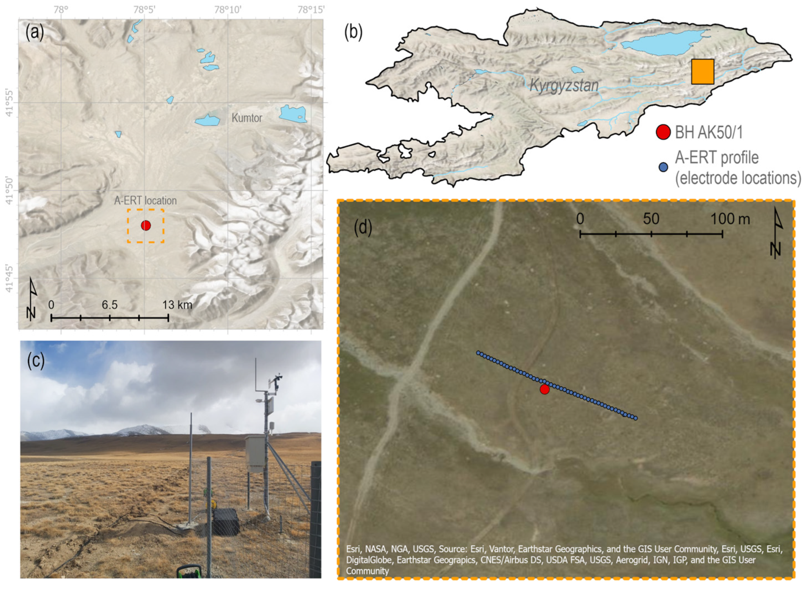
Figure 2.
The latest version of the TRACE (Time-lapse Resistivity Assessment for Critical Environments) autonomous Electrical Resistivity Tomography (A-ERT) monitoring system. The system comprises a lightweight 4-point Light 10 W resistivity meter integrated with the remote communication module (upper-right blue unit), a solar-powered battery system with charge controller (central blue unit), switch boxes for multi-electrode measurements (beneath the blue units), and military-grade connectors housed within a customized IP67 and MIL-STD-810F weather-resistant enclosure designed for long-term autonomous operation in harsh permafrost environments.
Figure 2.
The latest version of the TRACE (Time-lapse Resistivity Assessment for Critical Environments) autonomous Electrical Resistivity Tomography (A-ERT) monitoring system. The system comprises a lightweight 4-point Light 10 W resistivity meter integrated with the remote communication module (upper-right blue unit), a solar-powered battery system with charge controller (central blue unit), switch boxes for multi-electrode measurements (beneath the blue units), and military-grade connectors housed within a customized IP67 and MIL-STD-810F weather-resistant enclosure designed for long-term autonomous operation in harsh permafrost environments.
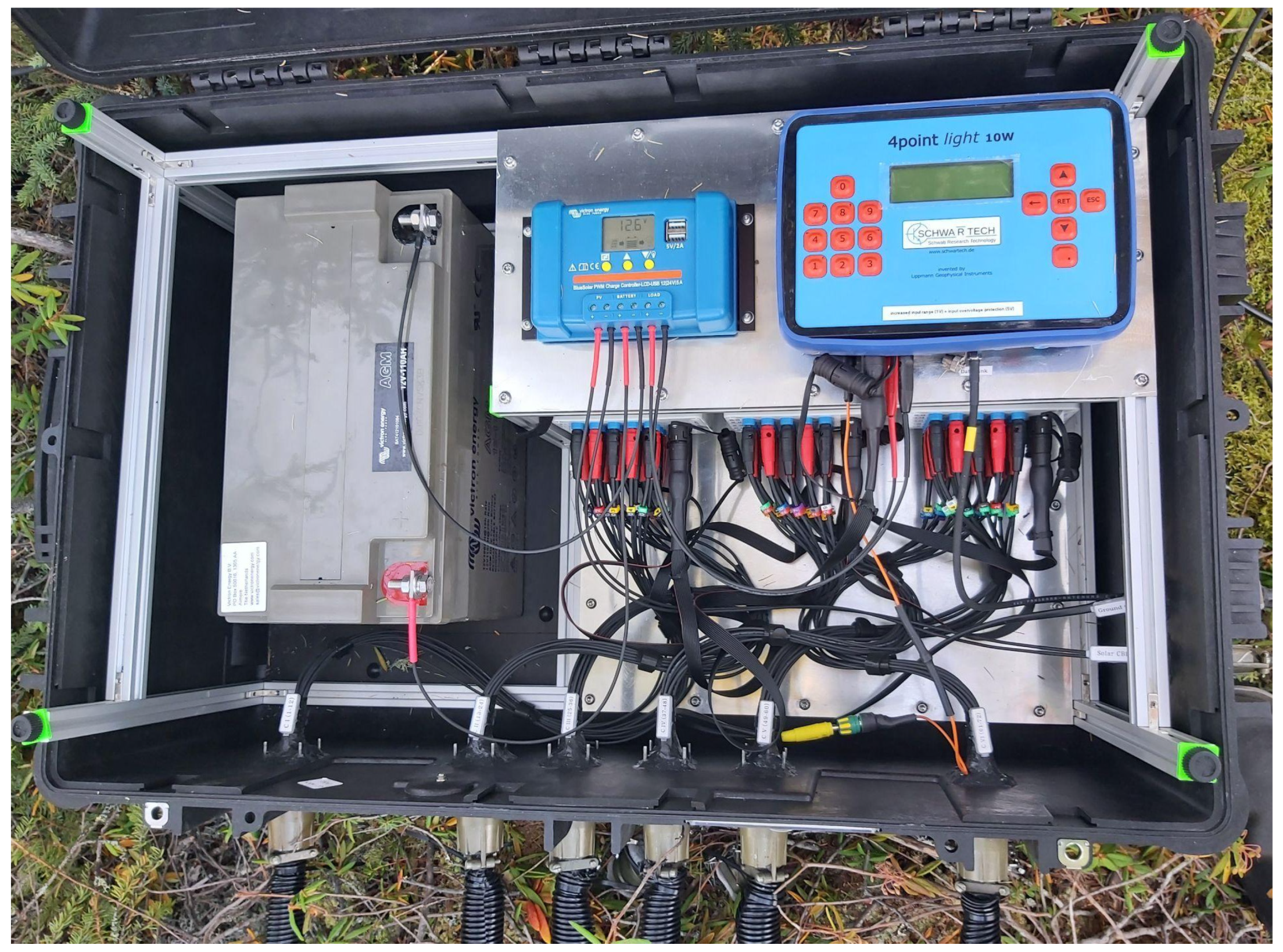
Figure 3.
Time series from October 2023 to August 2024 showing: (a) internal temperature recorded by the 4-point light 10 W resistivity meter within the TRACE setup; (b) battery voltage evolution during autonomous operation; and data-quality indicators including (c) the number of filtered data points removed from each dataset and (d) the RMS error of the inverted A-ERT models.
Figure 3.
Time series from October 2023 to August 2024 showing: (a) internal temperature recorded by the 4-point light 10 W resistivity meter within the TRACE setup; (b) battery voltage evolution during autonomous operation; and data-quality indicators including (c) the number of filtered data points removed from each dataset and (d) the RMS error of the inverted A-ERT models.
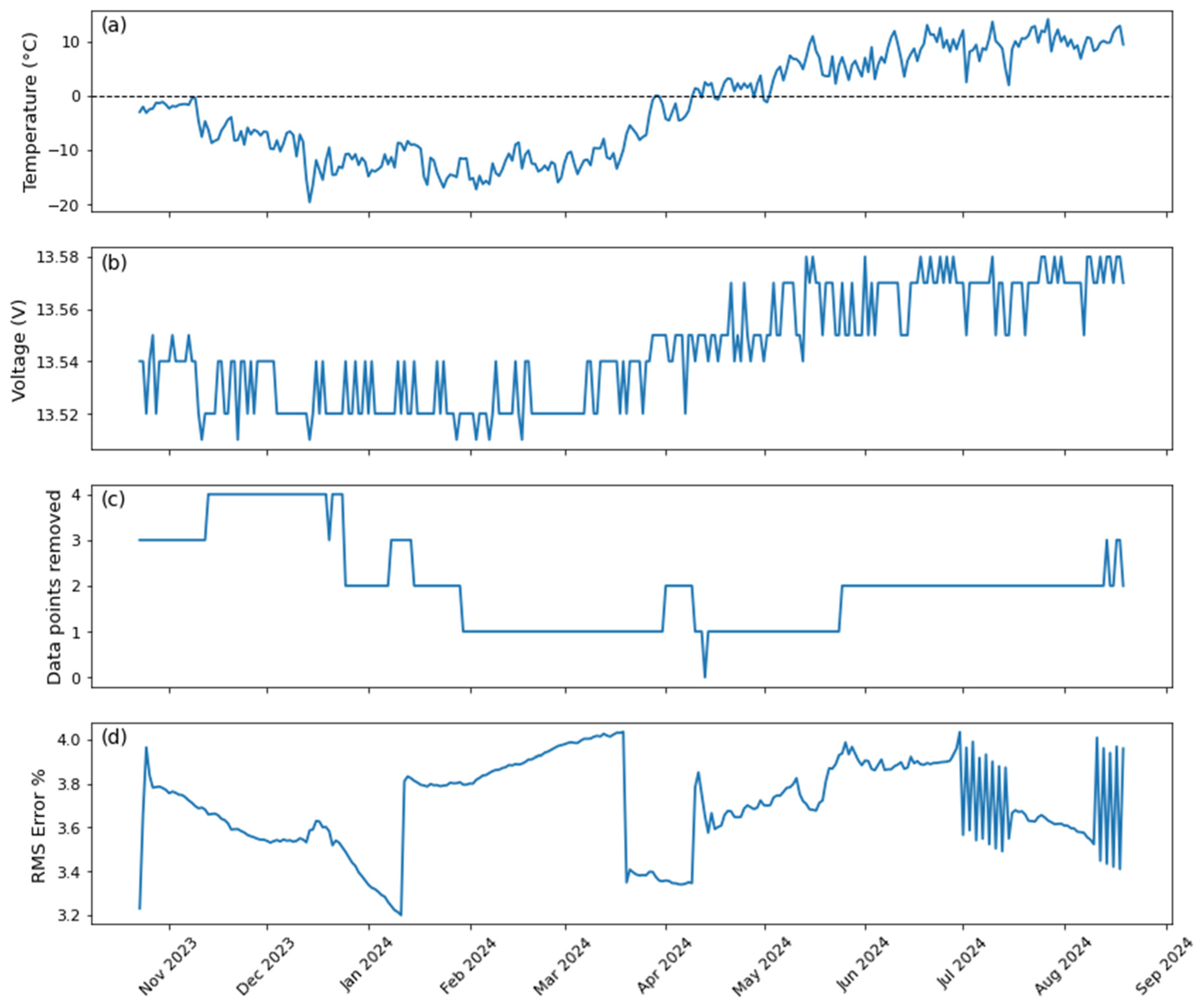
Figure 4.
Time series from October 2023 to August 2024 showing: (a) air temperature; (b) near-surface ground temperature at 0.5 m depth; and (c) Average apparent resistivity (ρa) at multiple electrode spacings. Blue shading indicates periods with daily maximum air temperature below 0 °C.
Figure 4.
Time series from October 2023 to August 2024 showing: (a) air temperature; (b) near-surface ground temperature at 0.5 m depth; and (c) Average apparent resistivity (ρa) at multiple electrode spacings. Blue shading indicates periods with daily maximum air temperature below 0 °C.
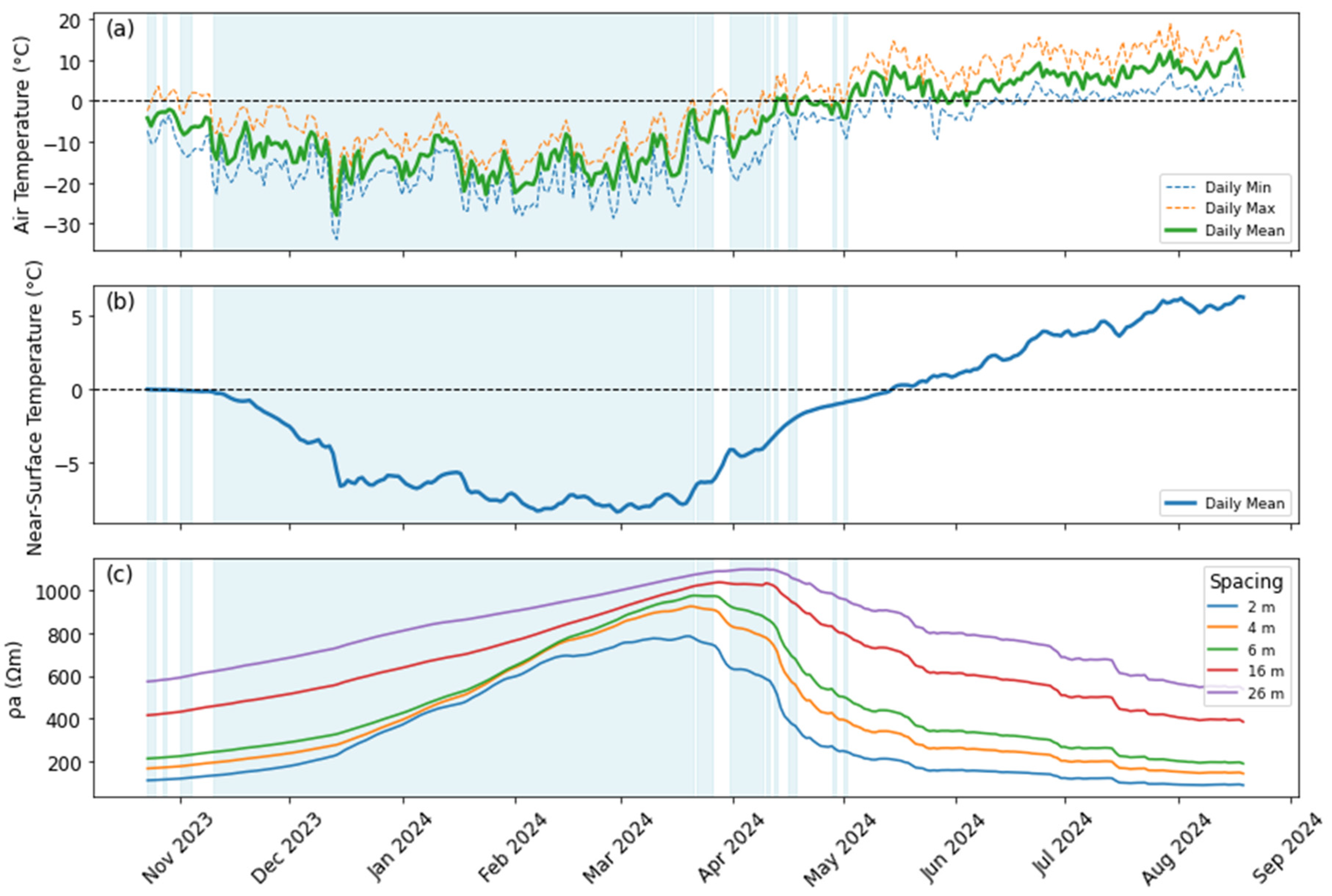
Figure 5.
Selected inverted 2D resistivity models illustrating the seasonal evolution of subsurface electrical resistivity between October 2023 and August 2024: (a) late October 2023, representing early freezing conditions; (b) mid-January 2024, corresponding to winter conditions; (c) mid-April 2024, during late winter to early spring transition; (d) early May 2024, representing the onset of thawing conditions; and (e) mid-August 2024, corresponding to late summer and maximum thaw conditions.
Figure 5.
Selected inverted 2D resistivity models illustrating the seasonal evolution of subsurface electrical resistivity between October 2023 and August 2024: (a) late October 2023, representing early freezing conditions; (b) mid-January 2024, corresponding to winter conditions; (c) mid-April 2024, during late winter to early spring transition; (d) early May 2024, representing the onset of thawing conditions; and (e) mid-August 2024, corresponding to late summer and maximum thaw conditions.
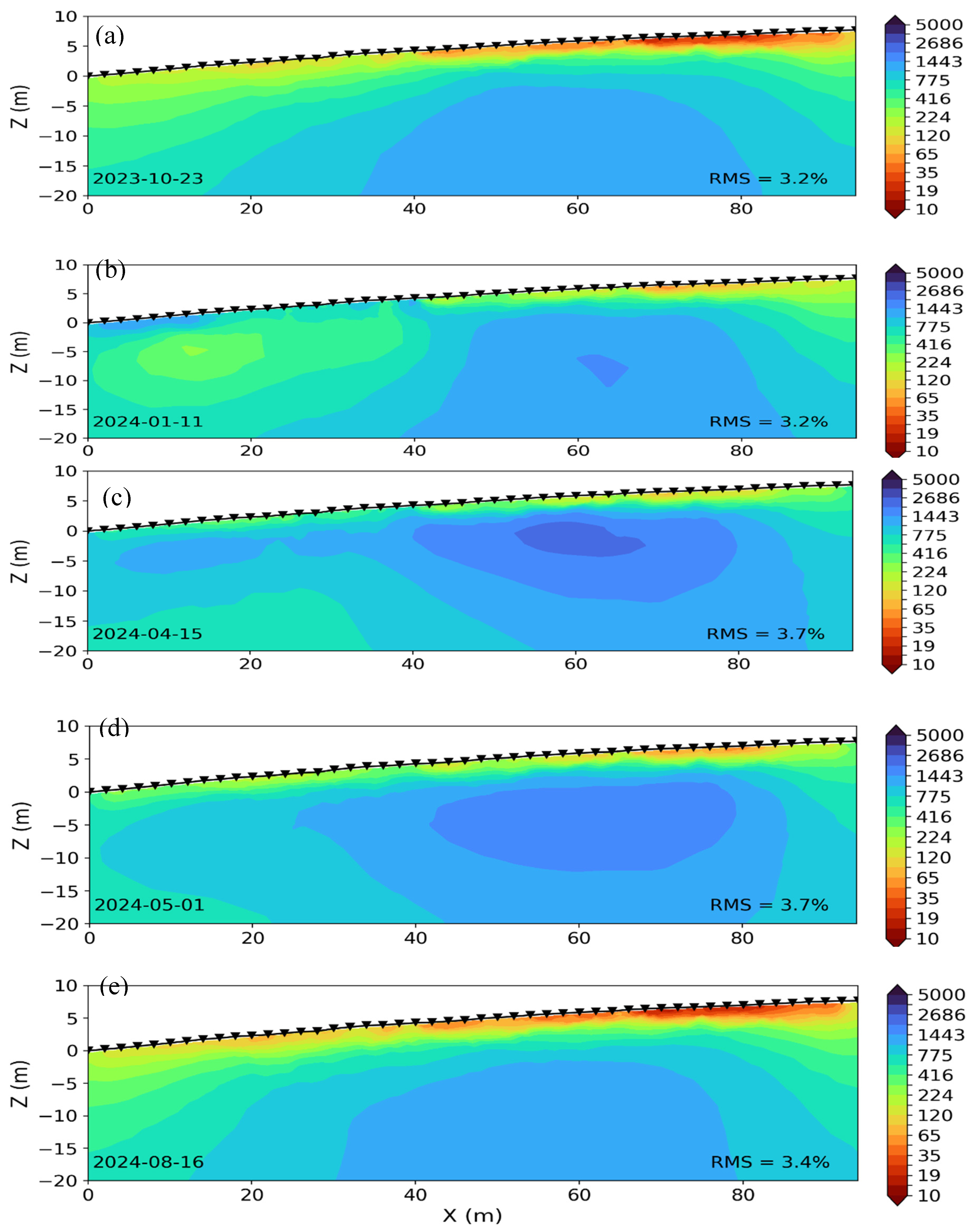
Figure 6.
Temporal evolution of ground temperature (blue) and extracted resistivity values (red) (left column) together with the corresponding temperature–resistivity relationships during cooling and warming periods (right column) at selected depths between October 2023 and August 2024. Panels (a–e) show the time series at depths of 1, 2, 3, 5, and 10 m, respectively, while panels (f–j) present the corresponding temperature–resistivity relationships. Dashed horizontal lines in panels (a–e) indicate the 0 °C isotherm. Only sub-zero temperature data are shown in the temperature–resistivity relationships (f) for the 1 m depth.
Figure 6.
Temporal evolution of ground temperature (blue) and extracted resistivity values (red) (left column) together with the corresponding temperature–resistivity relationships during cooling and warming periods (right column) at selected depths between October 2023 and August 2024. Panels (a–e) show the time series at depths of 1, 2, 3, 5, and 10 m, respectively, while panels (f–j) present the corresponding temperature–resistivity relationships. Dashed horizontal lines in panels (a–e) indicate the 0 °C isotherm. Only sub-zero temperature data are shown in the temperature–resistivity relationships (f) for the 1 m depth.
Disclaimer/Publisher’s Note: The statements, opinions and data contained in all publications are solely those of the individual author(s) and contributor(s) and not of MDPI and/or the editor(s). MDPI and/or the editor(s) disclaim responsibility for any injury to people or property resulting from any ideas, methods, instructions or products referred to in the content. |
© 2026 by the authors. Licensee MDPI, Basel, Switzerland. This article is an open access article distributed under the terms and conditions of the Creative Commons Attribution (CC BY) license (http://creativecommons.org/licenses/by/4.0/).
Copyright: This open access article is published under a Creative Commons CC BY 4.0 license, which permit the free download, distribution, and reuse, provided that the author and preprint are cited in any reuse.