

Submitted:
20 August 2026
Posted:
21 August 2026
You are already at the latest version
Abstract
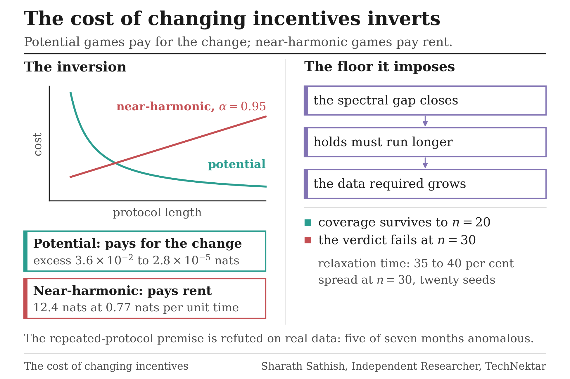
Logit revision dynamics on a finite game form a Markov jump process on the joint actionprofile, and moving the precision parameter λ drives that process out of its stationary state.This paper measures what the move costs. On the Hatano–Sasa split of entropy productioninto a housekeeping part and an excess part, instantiated exactly on the joint-profile Glaubergenerator, the cost structure inverts along the potential-to-harmonic axis of the Hodgedecomposition. Potential games have identically zero housekeeping, pay only for the change,and obey a discrete quasi-static law ⟨Y⟩∝1/K in the number of protocol steps, withmeasured exponents−1.02 and−0.94: they can be driven arbitrarily cheaply. Near-harmonicgames pay a rent per unit time whether or not they are driven, accumulating 12.4 nats ofhousekeeping at a burn rate of 0.77 nats per unit time at harmonic fraction α= 0.95, whiletheir excess collapses three decades across the same family, from 3.6 ×10⁻² to 2.8 ×10⁻⁵nats. The mechanism behind the collapse was identified by an information-gain-driven probecampaign as a path-length floor over the sequence of steady states, at posterior 0.996 onprobes lying in the well-relaxed regime, where the winning hypothesis is exactly true byconstruction, so that the posterior identifies a regime and is not an empirical discriminationbetween four live possibilities; the floor carries a held-out median residual of 0.002 dexon nineteen unconsumed probes, and a per-step path-aware recursion predicts the excessto a held-out median of 0.076 dex and a worst case of 0.44 dex. The second result is acost of measurement: because the relaxation time sets the hold length a data-side readingrequires, and the spectral gap closes as precision concentrates, the data a real system mustsupply grows precisely in the regime of interest. That floor is quantified with a physicalgate at four relaxation times per hold, a twenty-seed unbiasedness and coverage study, anda decomposition showing that interval coverage survives to n = 20 trajectories while theinstrument’s own verdict does not, failing at n= 30 for every candidate error bar becausethe relaxation-time estimate carries a 35 to 40 per cent across-seed standard deviation atthat same n= 30, over twenty seeds. The empirical position is a refutation reported as such:applied to a real power market, the repeated-protocol premise the whole construction restson fails month by month, with five of seven months anomalous under seasonal drift, and theclosed daily-loop affinity of about 7.0 nats per day [6.22,8.50] stands as descriptive only, onout-of-scope states and with the fluctuation theorem uninformative on cycles. Every othervalue quoted above is a point recorded without an interval, against a project rule requiringone on each quantitative statement: the two intervals given attach to a fluctuation-theoremcheck that is a regression test and to a number reported as descriptive only.
Keywords:
quantal response equilibrium
; logit dynamics
; stochastic thermodynamics
; Hatano–Sasa relation
; potential and harmonic games
; entropy production estimation
1. Introduction
Strategic environments are not held fixed. Stakes rise and fall, information arrives, penalties are re-set, and the sharpness with which agents respond to payoff differences moves with all of it. In the quantal-response family that sharpness is a single parameter: the logit precision , which interpolates between uniform randomisation and best response [15,30]. A large empirical literature treats as a quantity to be estimated from choice data [4,16], and a theoretical one derives it from an information cost the agent pays for attention [14,29]. Both treat it as a number. The question this paper asks is what happens when that number is a schedule: what does it cost, in the thermodynamic sense, to change the incentives a strategic system runs under.
The question has a well-posed answer because logit revision dynamics on a finite game are a continuous-time Markov jump process on the joint action profile [5,35], and a Markov jump process driven by a time-dependent parameter is the canonical object of stochastic thermodynamics [42]. Its entropy production splits into a housekeeping part, which maintains a non-equilibrium steady state, and an excess part, which is the price of moving between steady states [13,19]. Applied to a ramp, the split answers the question directly: the excess is what the change costs, and the housekeeping is what the system was going to spend anyway.
Why the answer is not uniform across games.
The split is not uniform across games because the underlying process is qualitatively different at the two ends of the Hodge decomposition of the game [8]. When the game admits an exact potential [31,34], the Glauber chain satisfies detailed balance with a Gibbs stationary law, the housekeeping term is identically zero, and the only cost of a protocol is the excess, which vanishes in the quasi-static limit. When the game is near-harmonic, the same dynamics settle into a circulating non-equilibrium steady state whose maintenance costs something per unit time, and that cost is paid whether or not anything is being changed. The harmonic fraction of the normalised game is therefore the coordinate along which the cost structure of driving inverts. The stochastic-thermodynamics literature has no such coordinate, because it has no games; the game-theoretic literature that does have the coordinate uses it to study convergence and recurrence of learning dynamics [2,26], not the cost of moving the parameters.
The two contributions, and where the evidence is thin.
The first contribution is the inversion itself, measured on a pre-registered scan across an -indexed family. The second is a cost of measurement, and a referee from stochastic thermodynamics will find it the more useful of the two. A data-side reading of the excess needs each hold in the protocol to be long enough that the occupation it supplies is the steady state of that hold, and the length required is set by the relaxation time, which is the inverse of the generator’s spectral gap. That gap closes as concentrates the stationary law. So the amount of data a real system must supply before its excess dissipation can be read at all grows precisely in the regime where the excess is interesting. That statement is instrumented: a physical gate at four relaxation times per hold, a seed study that separates estimator bias from interval coverage, and a small-n extension that was attempted, refused by its own pre-registered guard, and partly retracted.
The empirical position is a refutation and this paper reports it as the headline, not as a limitation. The construction assumes a repeated protocol: many realisations of the same schedule, so that occupations can be pooled. Pointed at a real power market, that premise fails month by month, with five of seven months anomalous under seasonal drift. What survives is a descriptive number on a closed daily loop, on states that are outside the certified scope, with the fluctuation theorem uninformative on cyclic paths.
Relation to the companion papers.
The stationary reading of these same chains, in which response asymmetry and dissipation are shown to be two independent coordinates of a non-equilibrium steady state, together with the phase map of criticality in and the stationary detailed-balance reading of the day-ahead power market, is the subject of a companion paper [38] and is not restated here. The library that computes every meter used below, its calibration against systems whose correct reading is fixed in advance, and the trajectory estimators of stationary entropy production, are the subject of a second companion paper [37] and of the package itself [36]. This paper is entirely about driving, which neither companion has vocabulary for.
Contributions.
Concretely, this paper reports the following.
- C1.
-
The driving-cost inversion.On a pre-registered ramp across an -indexed family, the excess obeys a quasi-static law and collapses three decades in , while accumulated housekeeping is identically zero on potential games and grows with elapsed time at the near-harmonic end (Section 5).
- C2.
-
A mechanism with a held-out model and a named failure mode.The collapse is a path-length floor over the sequence of steady states the protocol visits, bracketed against the frozen divergence and modelled by a per-step path-aware recursion that repairs the loop-path failure of the single-gap crossover (Section 6).
- C3.
-
A measurement-cost floor.
- C4.
-
A refutation on real data, reported as the empirical headline.The repeated-protocol premise fails month by month on real market data and what survives is descriptive only (Section 10), read against the null construction of Section 9.
What this paper does not claim.
That entropy production splits into housekeeping and excess is standard, and is not claimed here; the derivation in Appendix A is an instantiation, not a theorem. That a local response coefficient and a global dissipation functional can be inequivalent for Markov jump processes is likewise established [1], and is the companion paper’s territory and not this one’s. What is new here is that the cost of driving has a structure along a game-theoretic coordinate, that the structure inverts across that coordinate, and that the same spectral quantity governing the inversion also sets a measured floor on observability. Every quench number below is synthetic unless it is explicitly attached to market data, everything in the mechanism campaign is two-player, and the record’s action-count coverage, where it is recorded at all, is .
1.1. Structure of the Paper
Section 2 states what is standard in the stochastic thermodynamics of driven jump processes, separates the Langevin results from their jump-process generalisations, and marks the boundary between what is inherited and what is added. Section 3 instantiates the split on the joint-profile Glauber generator and defines the quench protocol as a staircase in with holds. Section 4 validates the instrument before it is used, including a disclosure that one of the two fluctuation-theorem checks is algebraically forced and therefore cannot catch a bug. Section 5 reports the pre-registered scan and states the inversion. Section 6 reports the mechanism campaign, the three successive excess models and their held-out errors, and two process failures. Section 7 derives and instruments the measurement-cost floor. Section 8 decomposes the small-n failure into two modes that a single statistic had conflated, and records a partial retraction. Section 9 states the null construction needed for observed series. Section 10 reports the real-market application and its refutation. Section 11 states threats to validity and limitations, and Section 12 states what a successor programme would have to run. Appendix A derives the split, Appendix B the two fluctuation theorems and the telescoping identity, Appendix C the protocol and the relaxation gate as reproducible procedure, Appendix D the three excess models side by side, and Appendix E the provenance of every figure, table and headline number, including the rows for which no artifact exists.
2. Background: Driven Markov Jump Processes
This section states the parts of the construction that are inherited. It is written so that a reader who knows stochastic thermodynamics can skip to Section 3 and a reader who knows game theory can find out exactly which results are being borrowed and from whom. The boundary between inherited and new is stated at the end of the section instead of being left implicit.
The process.
Let x range over a finite state space and let be transition rates depending on a control parameter . The distribution obeys the master equation
The split, and which paper it comes from.
The decomposition of Equation (2) into a housekeeping part that maintains the current steady state and an excess part that accounts for motion between steady states,
is due in its original form to Hatano and Sasa [19], and that paper is a Langevin result: it is stated for overdamped Langevin dynamics with a time-dependent control, and its proof uses the Fokker–Planck current. The generalisation to Markov jump processes, which is the form used throughout this paper because the object here is a jump process on a finite profile space, is due to Esposito and Van den Broeck [12] and is developed at length in the master equation formulation of Esposito and Van den Broeck [13]. The distinction matters beyond bookkeeping. Results in the Langevin class do not automatically transfer to the jump class, and there is a standing example: the Harada–Sasa equality relating dissipation to the integrated violation of the fluctuation-response relation [17] holds in the Langevin class and fails in the jump class, where response carries a frenetic contribution that is not a functional of entropy production [1]. This paper therefore cites Hatano and Sasa [19] for the relation and Esposito and Van den Broeck [12] and Esposito and Van den Broeck [13] for the jump-process statement it actually uses, and states which is which at every point of use.
The integral fluctuation theorems.
Two exact relations are used below. The first is the Hatano–Sasa integral fluctuation theorem. For a trajectory generated under a protocol , define the excess functional
accumulated at the switching times along the realised path . Then , where the average is over realisations of the protocol started from the stationary law of . The relation holds for every game in the family, including those far off detailed balance, and does not require the stationary law to be Gibbs. The second is the Jarzynski equality [24], which applies only where the stationary law is Gibbs, that is only on potential games, and whose detailed counterpart is the Crooks fluctuation theorem [9]. Both belong to the family whose jump-process members are catalogued by Esposito and Van den Broeck [12], and the general framing is that of Seifert [42]. The instantiation on the Glauber chain, with the exact form of the two relations checked here, is stated in Appendix B.
Reading dissipation from trajectories.
Where the generator is known, Equation (2) and Equation (3) can be evaluated exactly. Where only observed paths are available, the excess must be estimated, and the estimation of time-dependent entropy production from non-stationary trajectories is an active subject with known bias structure [32], as is the more general question of what can be bounded from coarse-grained observation [43]. A second inherited family bounds dissipation by the statistics of a current: the thermodynamic uncertainty relation of Barato and Seifert [3], proved for finite-time currents of steady-state Markov jump processes by Horowitz and Gingrich [21], states that the relative variance of any time-integrated current bounds the entropy production from below, so a current measured to a stated precision certifies a minimum dissipation and, read backwards, a target precision implies a minimum amount of observation. That family is standard, it is what a reader from stochastic thermodynamics will reach for when Section 7 costs a measurement, and Section 7 states there how the bound derived in this paper differs from it. The estimator used in Section 7 is the simplest member of the plug-in family, on pooled hold occupations, and its defects are reported, not assumed away.
What is standard and what this paper adds.
Everything above is standard. Equations (1)–(4), the two fluctuation theorems, the uncertainty relation of Barato and Seifert [3] and Horowitz and Gingrich [21], the non-negativity of both parts of the split, and the vanishing of the housekeeping part under detailed balance are all inherited, and the derivation in Appendix A is written as an instantiation on a particular generator and not as a new theorem. What this paper adds is a coordinate. The stochastic-thermodynamics literature parameterises driven systems by physical controls: a trap position, a chemical potential, a temperature. Here the driven control is the precision of a strategic response, and the systems being driven are indexed by a second parameter, the harmonic fraction of the game, which has no analogue in that literature at all. The results below are statements about how the standard split behaves as a function of that second coordinate, and about what the same coordinate does to the cost of measuring the split from data. The novelty is in the coordinate and in the measurement.
3. Setup: Logit Revision Dynamics as a Driven Chain
The generator.
A finite game has players , action sets with , and payoff tensors . Under logit revision dynamics, revision opportunities arrive at unit rate per player, and a revising player redraws an action from the softmax of its own payoff against the current actions of the others [5,35]. The resulting object is a continuous-time Markov jump process on the joint profile space with rates
and zero rate for transitions that move more than one player’s action. All softmax evaluations are performed in log space through log_softmax and logsumexp, never by exponentiating raw payoffs, and the payoff tensors are normalised before is applied, so that is a normalised precision [36]. Table 1 lists the symbols used throughout.

Table 1.
Notation.
| Symbol | Meaning | First used |
|---|---|---|
| N, m | players; actions per player | Section 3 |
| logit precision, normalised | Equation (5) | |
| harmonic fraction of the normalised game | Section 3 | |
| exact potential, where one exists | Equation (6) | |
| , | stationary law at ; at the k-th hold | Equation (3) |
| p, | actual distribution; tracked distribution at step k | Equation (13) |
| , , | total, housekeeping, excess entropy production rate | Equation (3) |
| Y | accumulated excess along a protocol, in nats | Equation (4) |
| K | number of steps in the staircase | Section 3 |
| hold duration; its estimate from data | Section 3 | |
| g, | spectral gap of the generator; at step k | Equation (12) |
| path-length floor | Equation (10) | |
| frozen divergence | Equation (11) | |
| n | number of protocol realisations available to the estimator | Section 7 |
The two ends of the family.
If the game admits an exact potential [31,34], the chain of Equation (5) is reversible with the Gibbs stationary law
the stationary probability current vanishes edge by edge, and Equation (2) is exactly zero [5]. If the game carries harmonic content in the sense of the Hodge decomposition [8], the same dynamics settle into a stationary but circulating state that dissipates at a positive rate. Families with a prescribed harmonic fraction are generated by unit-normalising the potential component of one random game and the harmonic component of another and mixing them as ; is therefore a construction parameter, exact by definition, and not a measured quantity. The terminological collision with the geometric decomposition literature should be defused once: the incompressible component of Legacci et al. [26] is the zero-divergence part of a deterministic flow, whereas harmonic here indexes maximal stochastic circulation of the revision chain, and the two are not the same object.
The split on this chain.
Substituting Equation (5) into Equation (3) gives the instantiation used throughout. The housekeeping part is the Schnakenberg form of Equation (2) evaluated with p replaced by the ratio weighting of the stationary currents, and the excess part is exactly at fixed ; Appendix A carries the derivation and the two verifications that the library performs on every call. The consequence that organises the paper follows immediately from Equation (6): on a potential game the stationary currents vanish identically, so
and the entire dissipation of a protocol is excess. There is no approximation in Equation (7) and no numerical threshold, and the numerical check that accompanies it is a regression test on the implementation. The equivalence has two halves, which are not equally cheap. That the housekeeping term vanishes identically if and only if the chain satisfies detailed balance is algebra, and Appendix A gives it. That detailed balance of the rates of Equation (5) holds if and only if the game admits an exact potential is the substantive half: it is the statistical-mechanical characterisation of this rate family given by Blume [5], which is stated for a common precision across players. That is the case used throughout this paper, and a family with player-specific precisions falls outside the statement and is not run here.
The quench protocol.
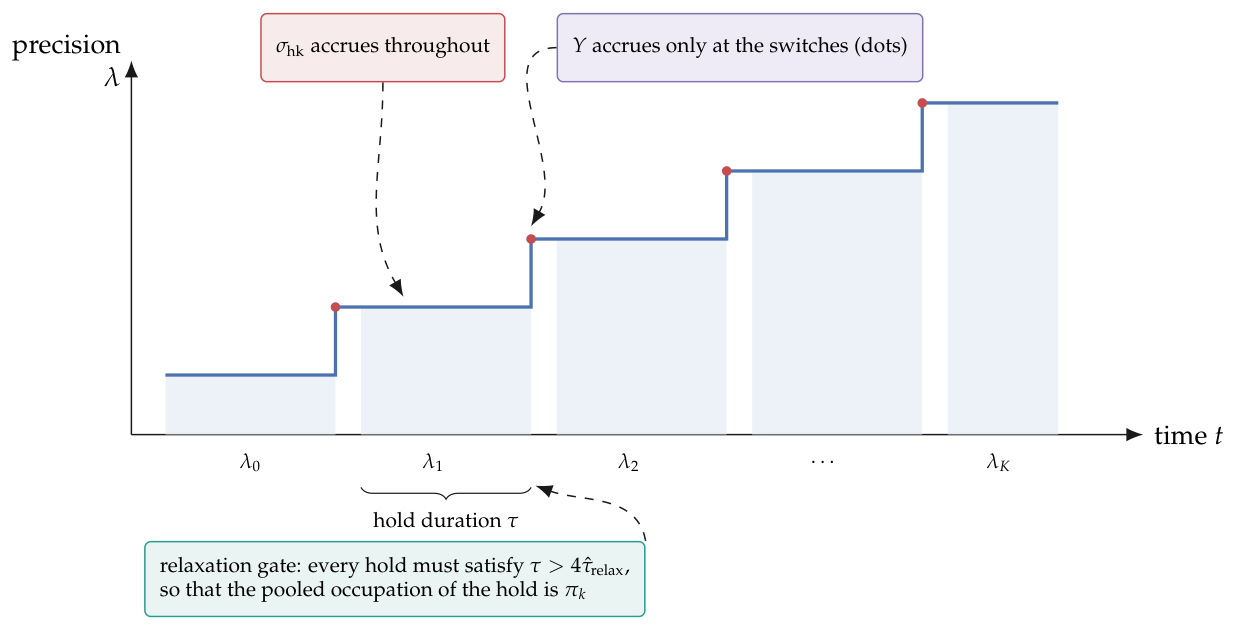
A quench protocol is a staircase in . The precision is held at until the chain has settled, stepped instantaneously to , held for a duration , stepped again, and so on through K steps to . The excess functional Y of Equation (4) accumulates only at the switches, because between switches the control is constant and the stationary law does not move; the housekeeping rate, by contrast, accumulates continuously throughout. By Equation (A3) that rate is evaluated on the actual distribution, which is still relaxing inside the hold, so it settles to a constant only once the hold is long compared with the relaxation time. That asymmetry is what makes the two parts respond differently to the same protocol, and it is the structural reason behind the result of Section 5. Figure 1 draws the staircase, the hold windows, and the relaxation requirement that Section 7 turns into a gate. Reading the protocol as a discrete traversal of the logit quantal-response correspondence in connects it to the homotopy interpretation of that correspondence [45]: the staircase is a coarse walk along a path the correspondence already defines, and K is how finely it is walked.
Figure 1.
The quench protocol as a staircase in the precision parameter, with hold windows shaded and the relaxation requirement annotated.
Figure 1.
The quench protocol as a staircase in the precision parameter, with hold windows shaded and the relaxation requirement annotated.
Scope of everything that follows.
The quench work is two-player. Where the record preserves an action count it is , and the one generalisation check that is recorded is the agreement of the family with the identified mechanism to per cent. The number of games per level in the quench scan, and the seed under which the scan was run, are not recorded anywhere in the repository; Appendix E says so per row instead of supplying a plausible value.
4. Validation of the Instrument Before It Is Used
Nothing in Section 5 is worth reading if the excess functional is computed wrongly, so the checks come first, and so does the disclosure that one of them is weaker than it looks.
The two identities that were checked.
Unit thermo.protocols evaluates both integral fluctuation theorems on the joint-profile chain. On potential games, where Equation (6) makes the stationary law Gibbs, the Jarzynski equality [24] takes the explicit form
and it holds at machine precision. On every game in the family, including those far off detailed balance where Equation (8) has no content because no potential exists, the Hatano–Sasa relation for the functional of Equation (4) holds at machine precision as well. Both results are recorded in the project’s claims ledger under row K3, tier exact. The universality of the second identity across the family is the reason the excess is a usable coordinate at all: it is the one quantity in this paper whose correctness does not depend on the game being close to equilibrium.
The check that cannot fail.
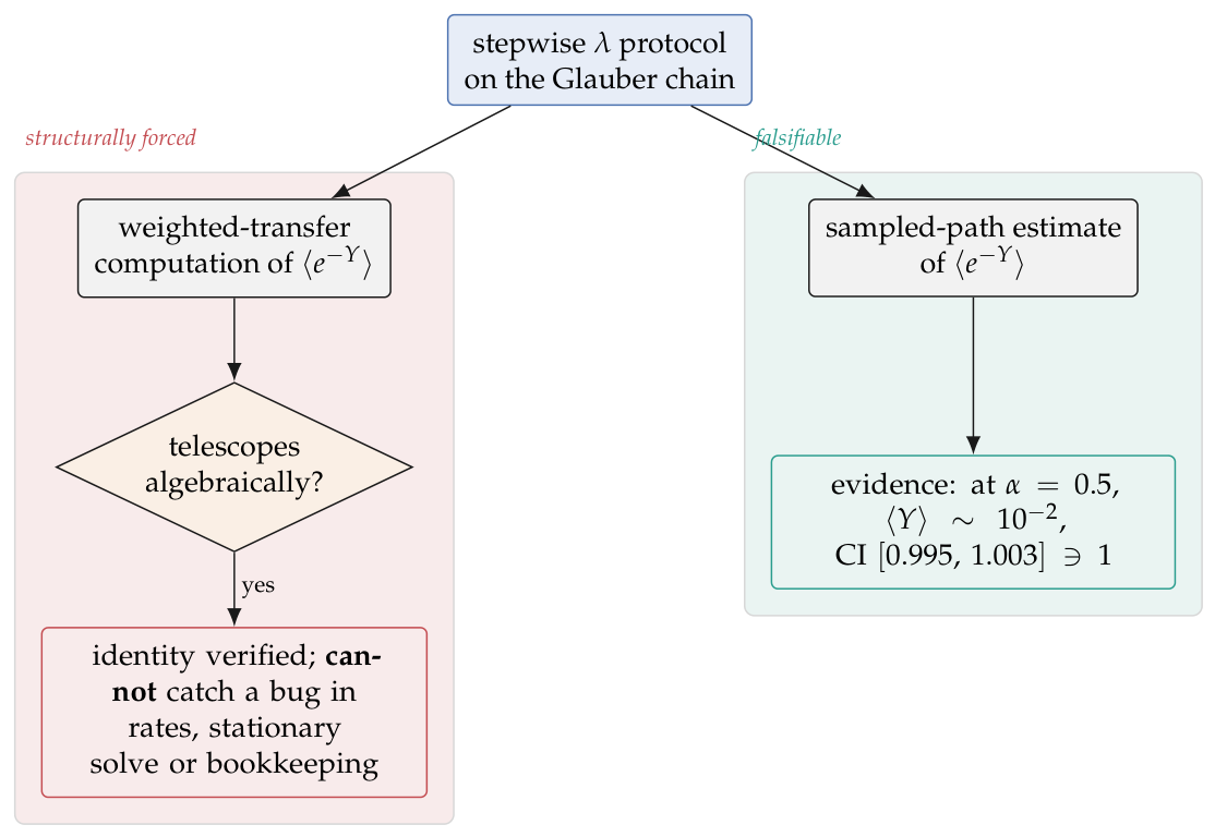
The two identities are not equally informative, and a reader who works this out independently will discount everything downstream of it, so it is stated here instead of in an appendix. For a stepwise protocol, the weighted-transfer computation of evaluates the average by propagating the reweighted distribution across each switch and each hold in turn. Written out, the stationary-law factors introduced at switch k cancel against those removed at switch , and the product telescopes to 1 identically, for any rates whatsoever. Appendix B gives the cancellation explicitly. The consequence is that this check verifies an algebraic identity about the implementation of a telescoping product and cannot detect an error in the rates, in the stationary solve, or in the protocol bookkeeping. It is a regression test, not evidence.
The check that can fail.
The correctness test is therefore the independent sampled-path evaluation: simulate realisations of the protocol, accumulate Y along each realised trajectory using only the states the trajectory visited, and average over realisations. This estimate has genuine sampling error and is sensitive to every part of the implementation. It was powered at , where so that the exponential average is not dominated by a single tail realisation, and it returned a confidence interval of , which contains 1. This is the only fluctuation-theorem number in the paper that constitutes evidence, and it is the only quench number in the repository with a named artifact, protocol_ift_checks.json.
Figure 2 shows the two checks and their standing side by side, with the telescoping branch drawn as the weak path.
Figure 2.
The two fluctuation-theorem checks and what each can detect.
What the fluctuation theorem is retained for.
Because the identity check is forced, the fluctuation theorem is not used anywhere below as a certification of correctness. It is retained as an anomaly detector on the data-side estimator of Section 7, where it does have power against one specific failure: input that is not truly stepwise, for which the telescoping premise is false and the identity therefore breaks. That use is tested. Its inadequacy for the different job of detecting estimator bias is the subject of Section 7, and the number that settles it is that a 45 per cent bias can sit behind a fluctuation-theorem value of .
5. The Driving-Cost Inversion
The scan and how it was committed.
The scan was pre-registered: its predictions were written into the run configuration before the run, so that a disagreement between prediction and outcome could not be resolved after the fact. The registration carries one defect. The commit intended to fix the predictions in the repository history before execution aborted on a pre-commit hook failure, so the registration and the results entered the history in the same commit, and the audit gap that creates is recorded as an audit gap. The predictions themselves are visible in the configuration and were not edited between the failed commit and the successful one, but a reader who requires the ordering to be provable from the history alone cannot have it here.
The protocol ramped from to 3 as a staircase of the form drawn in Figure 1, applied across the -indexed family of Section 3. Two families of measurement were taken: the excess as a function of the number of steps K at fixed endpoints, and the accumulated housekeeping as a function of protocol duration.
The quasi-static law.
Refining the staircase at fixed endpoints reduces the excess, and the reduction follows the discrete quasi-static law
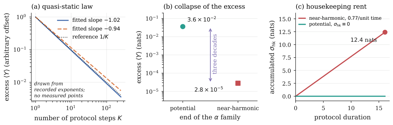
with measured exponents and on the two fits recorded. The exponents are not identical and the record does not attach either to a particular , so the statement supported is that the law is to within the spread of the two fitted values, not that a systematic dependence of the exponent on has been measured. Equation (9) is what makes the phrase driven arbitrarily cheaply precise: on a potential game the housekeeping term is identically zero by Equation (7), the excess is the whole cost, and the excess goes to zero as the staircase is refined. Total dissipation for the same change of incentives can be made as small as desired by making the change slowly enough, in as many steps as one is willing to pay for in time.
The collapse across the family.
At fixed K, the excess falls three decades as the game moves from the potential end of the family to the near-harmonic end, from to nats. Figure 3(b) plots the two recorded endpoints. This is the part of the result that is not obvious in advance, and it is the part Section 6 explains: as the stationary law becomes less sensitive to , the sequence of steady states the protocol must traverse becomes shorter in an information-geometric sense, and the excess is a functional of that path length.
Housekeeping, and why the total is the wrong number.
The accumulated housekeeping over the protocol reaches nats at and is linear in protocol duration in the well-relaxed limit, where every hold is long compared with the relaxation time of the generator at that hold’s precision. The qualification is load-bearing. By Equation (A3) the housekeeping rate is a functional of the actual distribution p through the actual current, and p is still relaxing towards for a time of order after each switch, so the rate is constant within a hold only once p has reached . Where the hold duration dominates that time, which is the regime the scan was run in, per-hold housekeeping is a constant rate multiplied by the hold length and the accumulation is linear; outside it the linearity is an approximation whose residual is not recorded. A total of nats therefore says as much about how long the protocol was run as about the game, and quoting it as a property of the game would be an error. The informative quantity is the rate, and the rate is nats per unit time at , in the same limit. Figure 3(c) plots the accumulation at that rate against the exactly zero line that Equation (7) guarantees at the potential end.
Figure 3.
Panel (a) draws the two recorded fitted exponents and panel (b) the two recorded endpoint values; panel (c) draws the housekeeping accumulation at the recorded rate, its marker placed at the quotient of the recorded total and that rate.
Figure 3.
Panel (a) draws the two recorded fitted exponents and panel (b) the two recorded endpoint values; panel (c) draws the housekeeping accumulation at the recorded rate, its marker placed at the quotient of the recorded total and that rate.
The inversion.
Putting the three measurements together gives the first result of the paper. At the potential end of the family, the cost of a protocol is entirely excess, and by Equation (9) the excess is proportional to the inverse of the number of steps: the system pays for the change, and by making the change finely enough the payment can be driven towards zero. At the near-harmonic end, the excess is three decades smaller still, so the change itself is almost free, but the housekeeping rate is positive and constant, so the system pays nats for every unit of time it exists, whether or not is moving at all. The cost structure has inverted: at one end of the Hodge axis the bill is proportional to how much the incentives change and can be made arbitrarily small by patience, and at the other end patience is precisely what is expensive, because the bill is proportional to elapsed time and is incurred by a system that is doing nothing.
Two consequences are worth stating at the point the result is claimed. The first is a design consequence: on a potential system, slow re-tuning of incentives is thermodynamically cheap, and the only reason not to re-tune slowly is the opportunity cost of the time. On a near-harmonic system the opposite holds, and any policy that lengthens the transition is paying rent for the privilege. The second is a caution about what has been measured. The inversion is a statement about two ends of one constructed family at two players, with the action count recorded as where it is recorded at all, and it inherits the scope fence of Section 3. It is also, in the project’s ledger, an extension of an existing row, not a claim carrying its own gate: no gate file, no adversarial review and no artifact exists for the unit that produced it, which Appendix E records row by row.
6. Mechanism: Why the Excess Collapses
The collapse in Figure 3(b) is the part of the inversion that needed explaining, and the explanation was produced by a probe campaign, not by inspection. This section reports the campaign, the model it produced, the model’s named failure mode, the repair, and two process failures that belong in the body because both changed what was believed.
The campaign.
Four quantitative hypotheses were written down, each required to predict the outcome of every candidate probe before any probe was run: a payoff-scale fold, in which the collapse is a coordinate artefact of how the family is normalised; a non-equilibrium-sensitivity floor, in which the excess is bounded below by the information-geometric length of the path of steady states the protocol traverses,
a spectral-gap lag model, in which the excess is set by how far the actual distribution falls behind the moving steady state; and a quadratic strawman included so that the selector had a hypothesis that ought to lose. Probe selection maximised the expected information gain about which hypothesis is true [27], in the mutual-information form used for Bayesian active learning [22], and beliefs were updated by Bayes’ rule after each probe. Unit estimate.bayes ran the loop.
The most discriminating probe available was at , carrying nats of expected information, and the campaign resolved in one round: the floor hypothesis at posterior . The verdict was then validated on all 19 probes the campaign had not consumed, at a median residual of dex.
Scope of what the campaign established.
In the well-relaxed regime, where every hold is long compared with the relaxation time, is exact in the limit, so within that regime the campaign did not discover a law: it identified which regime the scan had been run in and generalised the identification, with the family agreeing to per cent. At fast quenches the picture is different, lag dominates, and the floor formula fails by design. Stating this is what makes the posterior of interpretable: it is a high posterior on a hypothesis that is exactly true in one regime and knowingly false in another, and the informative content is the regime boundary, which is the subject of the next paragraph.
Table 2.
Hypothesis scoreboard for the mechanism campaign.
| Hypothesis | Content | Outcome |
|---|---|---|
| Payoff-scale fold | the collapse is an artefact of the family’s normalisation | not supported |
| Path-length floor | bounded below by Equation (10) | selected, posterior ; exact in the well-relaxed limit |
| Spectral-gap lag | excess set by how far p trails the moving | not selected as the leading term; recovered as the correction in Equation (12) |
| Quadratic strawman | excess quadratic in the step size | not supported |
The bracket.
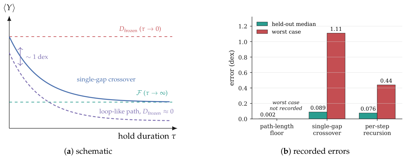
A second campaign closed the fast-quench remainder at first order. The validated picture is a bracket. As the hold duration grows without bound the excess falls to the path-length floor of Equation (10); as goes to zero the system cannot move at all during the protocol and the excess is the frozen divergence between the initial and final steady states,
where the upper end is exact at but is approached non-uniformly, so it is a bracket and not a first-order expansion. A single spectral-gap crossover interpolates between the two ends,
with g the spectral gap of the generator. On monotone paths of steady states this holds to about dex, with a held-out median error of dex.
Its failure mode, named.
Equation (12) compares only endpoints, so it fails when the endpoints are not representative of the path. That happens whenever the path of steady states is loop-like, with and substantial excursions in between, which is exactly the configuration at under a long ramp. There while the traversed path is long, and the formula underestimates by about one dex. That such paths exist under logit dynamics is not surprising: cyclic behaviour of logit dynamics in games is documented [20]. The failure is reported, not averaged into a summary error.
The repair.
A third campaign, unit science.quench_multimode, replaced the global endpoint comparison by a per-step, path-aware recursion. The tracked distribution relaxes towards the current steady state at the current gap,
with the gap at , and Y is accumulated along the tracked distribution instead of between endpoints. Because the recursion follows the path, the loop-like configuration stops being pathological: the excursions are traversed and counted. The recursion dominates the crossover on both summaries, at a median of dex against with games included, and a worst case of dex against . Table 3 and Figure 4 put the three models side by side; Appendix D states each one’s domain of validity in full.
Table 3.
The three excess models on their recorded errors.
| Model | Form | Median | Worst | Named failure mode |
|---|---|---|---|---|
| Path-length floor | Equation (10) | – | not a model outside the well-relaxed regime | |
| Single-gap crossover | Equation (12) | loop-like paths, about one dex | ||
| Per-step recursion | Equation (13) | none recorded |
Errors in dex. The floor’s median is the held-out residual over the 19 unconsumed probes of the first campaign, so it is not measured on the same held-out set as the other two rows and the three medians are not strictly comparable; a worst case for the floor is not recorded. The crossover and recursion medians are and on the comparison that includes games.
Figure 4.
Left: schematic of the bracket, the crossover and the loop-path failure; no measured curve is recorded, so no data are plotted. Right: the recorded held-out errors.
Figure 4.
Left: schematic of the bracket, the crossover and the loop-path failure; no measured curve is recorded, so no data are plotted. Right: the recorded held-out errors.
Two process failures.
Both are reported here instead of in a limitations paragraph, because both changed a conclusion. The first is a selector failure. In the second campaign the probe selector stopped after a single probe, confident in a winner, and the pre-registered held-out guard refused the verdict and returned winner_failed_validation. The guard was written before the campaign, precisely so that a confident selector could not close a question by itself, and it fired. The lesson is now a min_probes stopping gate in the loop, so that no verdict can be issued from a single probe regardless of posterior. The second is a retraction. The third campaign’s first result was a two-mode model, reported internally as an improvement, and it was withdrawn on adversarial review as an implementation artefact. The corrected two-mode model was then rebuilt and it still loses to the single-mode recursion of Equation (13): truncating the fast remainder at each switch turns out to err more than damping the whole deviation at the gap rate. The two-mode result does not appear in Table 3 because it is retracted.
7. Reading the Excess from Data, and What It Costs
Everything so far uses the generator. A real system supplies states, not rates, so the excess must be estimated from observed occupation. This section states the estimator, the certification arc that made it trustworthy and the self-check that did not, and then the second result of the paper: the data a system must supply before its excess can be read grows in exactly the regime where the excess is interesting.
The estimator.
Unit thermo.hs_estimator implements the plug-in form of Equation (4). Each hold’s observed occupation is pooled into an empirical stationary law , and accumulates at the switch states, over n realisations of the same protocol. The estimator has one structural requirement, which is what the rest of this section is about: the pooled occupation of hold k has to be the steady state of hold k, and it is not unless the hold is long compared with the relaxation time of the generator at .
The certification arc, and the self-check that failed to be one.
The first adversarial review of the estimator was withheld rather than granted, on the ground that the natural self-check was structurally insufficient. That self-check was the fluctuation theorem: if then the estimator must be right. It is not sufficient, and the number that settles the question is this: a 45 per cent bias can hide behind a fluctuation-theorem value of . The reason is that the exponential average is dominated by the small-Y realisations, and a bias that shifts the bulk of the distribution can leave that average close to 1. A reviewer who accepts a fluctuation-theorem value as certification of an estimator will accept a wrong estimator.
What followed is the part of the arc worth recording. Two statistical suspects were pursued and refuted, and the defect that was eventually found was not statistical at all: a missing pre-quench window, which silently dropped one jump term from the accumulation. With that corrected, a 20-seed study showed the estimator unbiased with calibrated intervals, covering the truth in 20 of 20 seeds at nominal 95 per cent. A count of 20 out of 20 at nominal 95 per cent is consistent with correct coverage but does not by itself distinguish 95 per cent from higher; the Wilson interval for that count [47] runs from about to , so the study demonstrates that coverage is not badly below nominal, and not that it is exactly nominal. The review was then granted and the unit is recorded as certified in the project ledger. Certified carries exactly that meaning wherever it appears in this paper: recorded as certified in row K3 of the project’s claims ledger. It does not mean a gate file exists. No unit behind this paper carries one, as Section 11.3 and Appendix E record unit by unit.
The gate is physical, not statistical.
The working gate that followed is not a p-value and not a sample-size rule. Every hold must exceed four times its own autocorrelation-estimated relaxation time,
and a protocol containing any hold that fails Equation (14) is refused and not reported with a caveat. Appendix C states the gate as procedure. The fluctuation theorem is retained alongside it as an anomaly detector, in the one role where it does have power: it fires on input that is not truly stepwise, which is a real failure mode for observed series that have been segmented into holds by a rule instead of by a controlled experiment.
The measurement-cost result.
Equation (14) is where the two halves of this paper meet. The relaxation time of a finite Markov chain scales as the inverse spectral gap of its generator, for some constant c that this record does not fix, so the total observation time a single realisation of a K-step protocol needs is
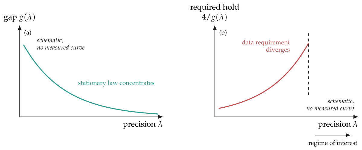
The first inequality is the gate rule of Equation (14) applied hold by hold, with the factor of four the gate’s working constant. The second step is the scaling identification, and c is unrecorded, so Equation (15) is a scaling statement in g and not a bound with a calibrated constant. The gap is not constant along the ramp. As grows the logit response sharpens, the stationary law concentrates on a shrinking set of profiles, and escape from that set becomes exponentially unlikely, so falls and grows. That concentration is the same mechanism the stationary companion paper reports as equilibrium concentration in the response operator [38]. Equation (15) therefore says that the required hold lengths, and with them the observation time, grow along the ramp, and grow fastest at its sharp end.
High precision is the interesting regime: it is where the quantal response approaches best response, where equilibrium selection bites, and where a change in incentives has the largest behavioural consequence. It is also the regime in which Equation (15) makes the data requirement diverge. Quench dissipation is hardest to measure exactly where a strategic system is most worth measuring. Figure 5 draws the two curves whose product is the difficulty.
Figure 5.
Schematic: the spectral gap closes as precision concentrates the stationary law, and the hold length demanded by Equation (14) grows as its reciprocal. No measured gap-against- curve is recorded.
Figure 5.
Schematic: the spectral gap closes as precision concentrates the stationary law, and the hold length demanded by Equation (14) grows as its reciprocal. No measured gap-against- curve is recorded.
Relation to the thermodynamic uncertainty relation.
A family of inherited results already says that reading a dissipation costs data, and the difference has to be stated so that Equation (15) is not read as a gate-specific restatement of it. The uncertainty relation of Barato and Seifert [3], in the finite-time form of Horowitz and Gingrich [21], bounds the relative variance of a time-integrated current of a steady-state process from below by a functional of the entropy production. It converts a required precision on a current into a required amount of observation through that current’s own fluctuations, and it is a variance statement about a stationary current. Equation (15) is a different quantity. It bounds no variance and says nothing about the fluctuations of : it is a hold-length requirement, because the plug-in form of Equation (4) needs each hold’s pooled occupation to be that hold’s stationary law, and the time that takes is set by the spectral gap. The failure it guards against is bias from an unsettled hold, and the failure an uncertainty relation guards against is an under-resolved current. The two are complements: an uncertainty relation would bound how many realisations a target precision needs once every hold is settled, and Equation (15) bounds how long a hold must be before the estimate it feeds is unbiased at all.
What Equation (15) is and is not.
It is an inequality assembled from the gate rule of Equation (14) and the standard scaling of the relaxation time with the inverse spectral gap, with the constant of that scaling unrecorded. It is not a measurement: no curve of g against for this family is recorded in the repository, which is why Figure 5 is a schematic and is captioned as one. What is measured is the consequence at the small-n end, where the data supply is fixed by the world and cannot be increased: a month of market data supplies about 30 realisations against a certified floor of , and what happens at that sample size is the subject of Section 8.
8. Two Failure Modes That Looked Like One
The extension, and its refusal.
The certified floor of realisations is not reachable on a month of market data, which supplies about 30 trajectories, so an extension of the estimator to small n was attempted. It failed: the extension was not granted, and the extrapolation to quotable monthly windows drawn from the first pass at it is partly retracted in Section 10 and in Appendix E. What makes the episode worth a section is that the failure turned out to be two failures which a single summary statistic had conflated, and separating them changed what the remaining lever is.
Coverage survives; the verdict does not.
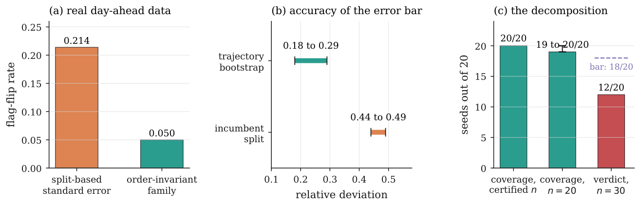
Interval coverage is intact well below the certified floor. At the intervals covered in 19 to 20 of 20 seeds, at a width of about times the bootstrap standard error. The estimate a month of data yields is therefore sound as a number with an interval around it. What fails at that sample size is the instrument’s own verdict: the Boolean the gate emits about whether the holds were long enough for the reading to be admitted. Agreement between that verdict and the exact settling status at fails for every candidate error bar tested, the best reaching 12 of 20 against a bar of 18 set before the comparison. Figure 6(c) plots the decomposition. A reading of the number and a reading of the admit-or-refuse decision are therefore two different reliability questions, and only the first survives at .
Figure 6.
Recorded values from the small-n and gate-standard-error studies: flag-flip rate under null day-order shuffles in (a), relative deviation from an oracle standard error in (b). The dashed threshold in (c) applies to the verdict bar only.
Figure 6.
Recorded values from the small-n and gate-standard-error studies: flag-flip rate under null day-order shuffles in (a), relative deviation from an oracle standard error in (b). The dashed threshold in (c) applies to the verdict bar only.
The permutation argument.
The decomposition came from a physical invariance. The order in which independent trajectories are listed is not a property of the system, so permuting that order must leave every verdict unchanged. It did not. Restricting the permutation so that it preserved the composition of the i::4 interleaved split, which the incumbent implementation used to estimate the standard error of the relaxation time, made the instability largely vanish. That is a localisation, not a repair: it identifies the split as the carrier of the order dependence, and thereby separates an implementation choice from anything about the physics of the chain.
The order-invariant family.
Replacing the split with estimators that cannot depend on trajectory order confirmed the diagnosis. Three were built: a leave-one-out jackknife computable in from the autocorrelation’s sufficient statistics, an analytic delta-method propagation, and a trajectory bootstrap [11]. Under null permutations the flag flips fall to zero at every n. On real day-ahead price data the flip rate under physically-null day-order shuffles falls from to , and the worst single month collapses from 17 of 20 to 0 of 20. The magnitude of what a standard-error choice controls is worth stating precisely: on one real month the choice of standard error moves an admit-or-refuse decision while leaving the point estimate identical to six decimal places. Nothing about the data changed; the instrument’s verdict about the data did.
Why the remaining failure is structural.
Fixing the flags did not fix the verdicts. Measured against an oracle standard error computed from independent replicates, the trajectory bootstrap is the most accurate of the four candidates, at to relative deviation against to for the incumbent, and it is still the case that agreement with exact settling status at fails for every candidate. The reason is that the quantity whose error is being estimated is itself unstable: the relaxation-time estimate carries an across-seed standard deviation of 35 to 40 per cent of its own value at . An accurate error bar must report that variance, and a gate that reports it must refuse holds that are in fact settled. Better error bars therefore make the verdict more conservative, not more accurate, which is the correct behaviour and is also why the lever is elsewhere: the remaining lever is a lower-variance estimator of the relaxation time, not a better standard error for the one in place.
The second, independent order dependence.
The same permutation argument then exposed a second order dependence, in the interval bootstrap itself, and there the obstruction is structural and not implementation-bound. The gate emits a hard Boolean by thresholding a Monte-Carlo interval; when the interval’s bound sits at the threshold, the Boolean inherits the Monte-Carlo noise, and no choice of seed removes it. Only two things do: reporting the margin instead of the Boolean, or driving the Monte-Carlo noise well below the distance to the threshold, which costs simulation. This is the same class of defect as the first, and it is not the same defect.
What was retracted.
The first pass at the small-n extension drew the conclusion that monthly windows would become quotable once the standard error was fixed. The standard error was fixed and the floor did not move. That extrapolation is partly retracted: what survives is the coverage statement, that the number and its interval are sound down to , and what does not survive is the inference that a fixed standard error makes a monthly verdict admissible. Table 4 lists the two remaining open modes as open.
Table 4.
Failure modes of the data-side reading.
| Mode | Mechanism | Diagnostic | Mitigation or status |
|---|---|---|---|
| Unsettled hold | pooled occupation is not because the hold is shorter than the relaxation time | autocorrelation-estimated per hold | the physical gate Equation (14); protocol refused, not caveated |
| Non-stepwise input | segmentation of an observed series into holds is not a controlled protocol | the Hatano–Sasa identity, which fires on such input | retained as anomaly detector; tested |
| Dropped jump term | a missing pre-quench window silently omitted one term from | 20-seed bias study against the exact value | fixed; estimator unbiased, coverage at nominal 95 per cent |
| Order-dependent standard error | the i::4 interleaved split makes depend on trajectory order | null permutation of trajectory order must not move a verdict | order-invariant family (jackknife, delta, bootstrap); flips → zero |
| Verdict inaccuracy at small n | carries 35–40 per cent across-seed SD at | agreement with exact settling status, bar | open: best candidate ; lever is a lower-variance |
| Boolean on a Monte-Carlo bound | a hard threshold applied to an interval whose bound sits at the threshold | the same permutation argument, applied to the interval bootstrap | open, structural: report the margin, or drive the noise below it |
The last two rows are open. The first four are closed, with the caveat that the first is a refusal rule and not a repair.
9. Null Construction for Observed Series
A reading taken from an observed price series is meaningless without a null that shares everything about the series except the property being tested. Three constructions failed before one worked, and each failure is now a permanent guard in the pipeline (unit domains.electricity). This section states them, because the refutation of Section 10 depends on the same machinery, and because the sequence is reusable by anyone reading irreversibility off a scalar time series.
Value-space discretisation is blind to loop irreversibility.
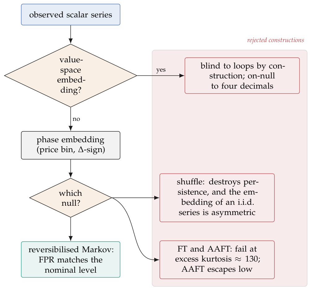
The obvious embedding of a price series discretises the price into bins and reads transitions between bins. That embedding cannot see a loop. A periodic drive retraces the same one-dimensional path, so the time-reversed series visits exactly the same set of value transitions as the forward series, with the same counts; the pair statistic is therefore identically at its null whatever the loop is doing. This is a proof, not an empirical finding, and it was unit-tested on a noisy sine and then confirmed on the real data, where the value-space reading sits on its null to four decimal places. The remedy is to embed in a space where direction is visible: the pair (price bin, sign of the increment), which distinguishes rising from falling passages through the same price.
Two ways a null can fail.
With the embedding fixed, the null must still be constructed. A plain shuffle of the series fails twice over. It destroys persistence, so the null series is not comparable to the data on the property that dominates the pair statistic; and the phase embedding of an independent series is itself structurally asymmetric, so the null is not even centred on reversibility. A Fourier-transform surrogate [44], which preserves the linear autocorrelation, fails on a different axis: locational marginal prices carry excess kurtosis of about 130, and Gaussianisation distorts the sign-flip rate that the phase embedding reads. The amplitude-adjusted repair [41] restores the marginal distribution, but it still cannot bracket the data’s direction-persistence, and the observed reading escapes the null band on the low side, which is neither a detection nor a certified null. Table 5 records the taxonomy.
Table 5.
Null classes, what each controls, and how each fails.
| Null class | Preserves | Failure | Verdict |
|---|---|---|---|
| Value-space embedding (any null) | the marginal price distribution | provably blind to loop irreversibility; reads on-null to four decimals | unusable |
| Plain shuffle | the marginal only | destroys persistence; the phase embedding of an i.i.d. series is itself asymmetric | fails twice |
| Fourier-transform surrogate | the linear autocorrelation | Gaussianisation distorts the sign-flip rate at excess kurtosis | fails on tails |
| Amplitude-adjusted surrogate | autocorrelation and marginal | cannot bracket direction-persistence; reading escapes low | partial repair |
| Reversibilised Markov | embedded pair counts and persistence, with the flux symmetrised | none identified; false-positive rate matches the nominal level | the deciding null |
The null that decides.
The construction that works is a reversibilised Markov surrogate on the phase embedding. Fit the pair counts of the embedded series, symmetrise the flux so that the fitted chain satisfies detailed balance exactly, and simulate from that chain. The result matches the data’s persistence by construction, because the persistence lives in the diagonal and near-diagonal counts, which symmetrisation does not touch, and it satisfies detailed balance exactly, so it is a null for the property being tested and for nothing else. Its false-positive rate on data that is truly reversible matches the nominal level, which is the calibration that licenses its use. Figure 7 draws the sequence as a decision path, with the two failed branches drawn to the side.
Figure 7.
The null construction as a decision path, with the rejected branches grouped.
What this machinery is used for here.
The stationary application of this null hierarchy, in which the day-ahead hourly series is tested for pair-level detailed balance, is reported in the companion paper [38] and is not a result of this one. What Section 10 uses it for is different: to establish whether the premise of a quench reading, that the observed series is a repetition of one protocol, holds at all.
10. Real-Market Application, and Its Refutation
What the application requires.
The estimator of Section 7 reads the excess of a repeated protocol. It pools the occupation of hold k across realisations to form , which is only meaningful if the realisations are repetitions of the same schedule. On a market series, the candidate realisations are days and the candidate holds are intervals within the day, so the premise is that successive days are repetitions of one daily protocol. Unit domains.electricity.quench tested that premise before reading anything off it, on locational marginal prices from the CAISO SP15 hub.
The premise fails.
Tested month by month, the repeated-protocol premise is refuted: five of seven months are anomalous, and the pattern is seasonal drift, not noise. Days within a month are not repetitions of one schedule, and months are not repetitions of each other. This is a refutation of the applicability of the whole construction to this series, and it is reported as the empirical headline of the paper, not as a limitation attached to a detection. The finding was rewritten after adversarial review; the version of record is the refutation.
What survives, and what it is worth.
One number survives, and it is descriptive. Treating the diurnal cycle as a closed loop, the loop affinity is about nats per day, with a block-bootstrap interval of ; block resampling is the appropriate resampling scheme here because the series is serially dependent within the day [25,33]. Three qualifications travel with that number and none of them is optional. First, the states on which it is computed are outside the certified scope of the estimator, so the certification of Section 7 does not extend to it. Second, the sample size is the one Section 8 analyses: about 30 trajectories against a certified floor of , which is a regime in which the interval is sound but the instrument’s admit-or-refuse verdict is not. Third, and most limiting, the fluctuation theorem is uninformative on cycles. On a closed loop , the telescoping structure of Appendix B returns its identity regardless of what the loop did, so the one check that would ordinarily be run on a quench reading has no power on this one. The affinity is therefore a description of the observed loop and not a measured dissipation with a certified error bar.
Why the refutation is the useful result.
Two readings of the same evidence were available. One is to report the nats per day as a detection with caveats, which is what the pre-registration would have counted as a success. The other is to report that the instrument’s own precondition failed on the first real system it was pointed at, and to state exactly how that is known. The second is what Table 6 does. It is also the more useful of the two for anyone intending to apply this construction to observational data, because the premise that failed here, that an observed series is a repetition of one controlled protocol, is not special to electricity prices: it is the premise every quench reading of an uncontrolled system needs, and it is not usually tested. Related work in industrial-organisation econometrics faces the structurally identical problem of testing whether a candidate conduct model is consistent with observed data before estimating within it [10], and reaches the same methodological conclusion, that the premise test comes first.
Table 6.
The empirical position, claim by claim.
| Claim | Status | Basis |
|---|---|---|
| Days are repetitions of one daily protocol | refuted | five of seven months anomalous; seasonal drift |
| Closed daily-loop affinity nats per day | descriptive only | block bootstrap; out-of-scope states; |
| Fluctuation-theorem check on the loop reading | uninformative | telescopes on a closed loop, Appendix B |
| Monthly windows are quotable once the standard error is fixed | partly retracted | the standard error was fixed; the floor did not move (Section 8) |
| A quench dissipation has been measured on a real market | not claimed | no row above supports it |
Priors from the literature that the refutation is consistent with.
Daily price paths in wholesale electricity are not repetitions of a fixed schedule, and there is an economic reason to expect that: cyclical price paths in oligopoly are generated by strategies whose phase is not pinned to the calendar [28], and algorithmic pricing systems change the schedule they implement as they learn [7]. The nearest empirical precedent for reading an entropy production rate off observed interaction data is the analysis of an experimental social-interaction system by Xu and Wang [48], which is a controlled setting, and the contrast with an uncontrolled market series is the point. Entropy-based equilibrium statistics have been fitted to economic cross-sections [39], but a cross-sectional fit does not establish the temporal repetition a quench reading needs.
11. Discussion, Threats to Validity and Limitations
11.1. What the Two Results Mean Together
The inversion of Section 5 and the measurement floor of Section 7 are governed by the same quantity. The housekeeping rate that near-harmonic games pay is a property of the stationary currents of the generator, and the spectral gap that sets how long a hold must be is a property of the same generator’s relaxation. A system whose stationary state costs a lot to maintain is a system whose steady state is strongly circulating, and a system whose precision is high is a system whose steady state is concentrated and slow to re-equilibrate. The first makes driving expensive; the second makes reading the expense expensive. There is no configuration in which the cost is large and easy to see.
That has a consequence for how such measurements should be designed. The temptation on observational data is to buy more samples. Equation (15) says the binding constraint is not the number of realisations but the length of each hold within a realisation, and the two are not substitutes: n short holds do not make one settled hold, because the bias from an unsettled hold does not average away across realisations. This is the reason the gate in Appendix C is physical, and it is the reason the small-n extension of Section 8 could not succeed by improving the statistics.
11.2. Threats to Validity
No confidence intervals on the headline numbers.
The most serious methodological gap in this paper is that the quench scan records point values without intervals. The exponents and , the excess endpoints and nats, the accumulated housekeeping of nats, the burn rate of nats per unit time, the posterior of , and the dex errors , , , , and are all recorded as points. The two exceptions are the sampled-path fluctuation-theorem interval and the block-bootstrap interval on the market affinity. The project’s own documentation requires an interval on every quantitative statement, and the quench line does not meet that requirement. The consequence is that no claim in Section 5 should be read as distinguishing, for example, an exponent of from one of ; what the evidence supports is the law and the direction and order of magnitude of the collapse.
Two players, and one recorded action count.
Everything in Section 5 and Section 6 is two-player. The only recorded generalisation check is the family agreeing with the identified mechanism to per cent. Nothing establishes that the inversion survives at three or four players, and there is a specific reason for concern that it might not: the stationary companion paper reports that the corresponding stratified design loses its low- baseline at [38]. That is a different measurement, so it does not transfer as evidence against the inversion, but it is the direction in which the first size test should be run.
One family construction.
The -indexed family is generated by one recipe, mixing a unit-normalised potential component of one random game with a unit-normalised harmonic component of another. Nothing here tests whether the inversion is a property of or a property of that construction. Because is a construction parameter and not a measured attribute, a family built by a different recipe at the same nominal is not guaranteed to reproduce the numbers.
The regime identification is not a discovery.
In the well-relaxed regime, is exact in the limit. The mechanism campaign’s posterior of therefore reflects a hypothesis that was going to be true in the regime the probes lived in, and the campaign’s genuine content is the identification of that regime plus the generalisation across the family. Section 6 says this at the point of the claim. A reader who reads the posterior as an empirical discrimination between four live possibilities in all regimes has read it too strongly.
The excess models are compared on unequal footings.
Table 3 lists three medians, but only two of them, against or against in the comparison that includes games, are measured on the same held-out comparison. The floor’s dex is the residual on the first campaign’s unconsumed probes and is not a competitor on the same set. No worst case for the floor is recorded.
The relaxation gate is calibrated on synthetic protocols.
The factor of four in Equation (14) is a working constant, not a derived bound. It was set on controlled protocols where the exact settling status is known, and its transfer to observed series rests on the assumption that the autocorrelation-based measures the same thing there. Section 8 shows that this estimator carries 35 to 40 per cent across-seed variability at , so the gate on observational data is being applied with a noisy input.
One hub, one market, one instrument application.
The refutation of Section 10 is on CAISO SP15 across seven months. It is not established for other hubs, other markets, or other candidate protocols within the same series; a different segmentation of the day might satisfy the premise where the diurnal one does not, and that has not been tried.
11.3. Limitations of the Record Itself
Three gaps in the project’s own record bear on how much of this paper is independently checkable, and they are stated once, here, and again per row in Appendix E.
First, almost none of the quench line has a committed artifact. protocol_ift_checks.json is the only artifact filename attached to any quench number anywhere in the repository. The scan of Section 5, the three campaigns of Section 6, the certification arc and seed study of Section 7, the small-n and standard-error studies of Section 8, and the market work of Section 10 have no artifact filename recorded.
Second, none of the quench units carries a gate file or an adversarial review recorded in the paper set: thermo.protocols, estimate.bayes, science.quench_regimes, science.quench_multimode, thermo.hs_estimator, thermo.hs_estimator.smalln, thermo.hs_estimator.gate_se and domains.electricity.quench are all absent from the provenance apparatus of the earlier drafts. Adversarial review did occur within the quench line, and Section 4, Section 6 and Section 7 each report a review that changed a conclusion; what is missing is the standing gate record, not the review.
Third, the successor-programme decision record that the project’s own programme document requires does not exist, and one finding cited in that document as an endpoint of the quench range has no entry anywhere in the repository. Appendix E names both gaps explicitly.
11.4. The Position this Paper Is in
This paper has a synthetic result, a methodological result, and no admitted empirical result. The inversion is measured, mechanistically explained and modelled to a stated worst case. The measurement floor is derived from the gate rule and instrumented at the small-n end. The one application to a real system refuted its own precondition. A reader deciding whether to use this construction on observational data should read Section 10 first and Section 5 second.
12. Conclusions and the Successor Programme
On logit revision dynamics, the thermodynamic cost of changing incentive precision is not a single quantity with a single scaling. It separates into a part that is paid for the change and a part that is paid for elapsed time, and which part dominates inverts along the potential-to-harmonic axis of the game. On potential games the housekeeping part is identically zero and the excess obeys a quasi-static law, so the whole protocol can be made arbitrarily cheap by refining it. On near-harmonic games the excess is three decades smaller, so the change itself is almost free, but the housekeeping rate is positive and is incurred whether or not anything is being driven. Table 7 carries the measured values with their scope. The mechanism behind the collapse is a path-length floor over the sequence of steady states the protocol traverses, and the per-step path-aware recursion of Equation (13) is the model with the smallest recorded worst case (Table 3).
Table 7.
The pre-registered scan: every recorded quantity, with its scope.
| Quantity | Value | Scope and status |
|---|---|---|
| Ramp endpoints in | staircase, K steps, holds between steps | |
| Quasi-static exponent, fit 1 | level not recorded; no interval recorded | |
| Quasi-static exponent, fit 2 | level not recorded; no interval recorded | |
| Excess, potential end of family | nats | fixed K; K not recorded |
| Excess, near-harmonic end | nats | fixed K; three-decade span |
| Accumulated housekeeping | nats | ; linear in duration in the well-relaxed limit, so protocol-length dependent |
| Housekeeping burn rate | nats per unit time | , well-relaxed limit; the quotable form of the row above |
| Housekeeping, potential games | 0 exactly | algebraic, Equation (7); regression test |
| Hatano–Sasa IFT, sampled paths | CI | ; the one falsifiable check |
Two players throughout. No confidence interval is recorded for any row except the last; Section 11 states what that costs.
The second conclusion concerns observability. The hold length a data-side reading requires is set by the relaxation time, the relaxation time scales as the inverse spectral gap, and the gap closes as precision concentrates the stationary law. The data a real system must supply therefore grows in the regime where the excess matters most. That floor is instrumented rather than asserted: the physical gate of Equation (14), a seed study of the estimator’s bias and interval coverage, and the decomposition of Section 8, in which below the certified sample size the number remains sound while the verdict does not, for the reason that the relaxation-time estimate is itself unstable across seeds.
The empirical conclusion is a refutation. On the one real market the construction has been pointed at, the repeated-protocol premise fails month by month under seasonal drift, and the closed daily-loop affinity that survives is descriptive only (Table 6).
The successor programme.
Four items follow, in the order in which they would change what can be claimed.
- Intervals and artifacts on the existing numbers. Nothing new has to be discovered to close the largest gap in this paper. The scan of Section 5 and the campaigns of Section 6 must be re-executed under fixed seeds with per-level resampling, so that every point value in Table 3 and Table 7 acquires an interval and a committed artifact, and every quench unit acquires a gate file and an adversarial review. Until then the numbers in this paper are point estimates from runs whose outputs are not independently inspectable.
- A measured gap-against-precision curve. Equation (15) is assembled from a gate rule and a standard identification, and Figure 5 is a schematic because no measured curve exists. The single cheapest experiment that would upgrade the measurement-cost result from an argument to a measurement is a sweep of the generator’s spectral gap against across the same family, with the implied hold length plotted beside the gate’s demand.
- A lower-variance relaxation-time estimator. Section 8 localises the remaining verdict failure in , whose across-seed standard deviation is 35 to 40 per cent of its own value at . Reducing that variance is the only lever identified that would move the certified floor, and it is a well-posed estimation problem independent of everything else here.
- A controlled system in place of an observed one. The premise that failed in Section 10 is a premise about control, and it holds by construction in a laboratory experiment where the incentive schedule is imposed. An experimental design in which is manipulated by changing stakes across rounds, with the schedule repeated, would supply exactly the repeated protocol the estimator requires, and would test the inversion where its precondition is satisfied instead of where it is not.
Two smaller items complete the list. The size test at three and four players is the one pass over the existing machinery that would tell whether the inversion is a two-player phenomenon, and the alternative family construction of Section 11.2 would tell whether it is a property of or of one recipe. Neither has been run.
Data Availability Statement
The library that implements every meter, generator and estimator used here is released as strataq [36] and its source, configuration files and regeneration targets are public [37]. The synthetic families of Section 3 regenerate from the recorded construction recipe. The quench runs of Section 5, Section 6, Section 7 and Section 8 have no committed output artifacts other than protocol_ift_checks.json; Appendix E records that gap row by row instead of naming files that do not exist. The market data of Section 10 are public locational marginal prices published by the system operator and are not redistributed with the repository.
Acknowledgments
The adversarial reviews reported in Section 4, Section 6 and Section 7 were run as an internal red-team process with the reviewer given the artefact and the claim and not the implementation rationale. Three of the results in this paper exist in their current form because that process refused an earlier version. Those reviews are recorded in the project’s claims ledger and not in gate files: no unit behind this paper carries one, which is why Section 7 defines certified as a ledger record and Appendix E lists the missing gates by unit. All numerical work is float64 throughout, with double precision enabled explicitly in the array backend. The library is strataq version [36], built on JAX [6], NumPy [18] and SciPy [46]. Figures are produced by Matplotlib [23] from the script make_figures.py that accompanies this paper, which plots only values recorded in the project’s own audit and claims ledger and draws no curve through unmeasured points. Diagrams are drawn in TikZ within the manuscript source. No literal numerical constant appears in library code; every parameter enters through a typed configuration schema. Implementation, experiment execution and manuscript preparation were carried out with substantial assistance from large language model coding agents, operating under the project’s gate, review and reproducibility rules. All claims, scope statements, retractions and limitations in this paper are the author’s. Every number reported here traces to a run recorded in the project’s claims ledger or audit; where the trace is incomplete, Appendix E says so.
Conflicts of Interest
The author declares no competing financial or non-financial interests. No funding was received for this work.
Appendix A. The Entropy-Production Split on the Joint-Profile Glauber Chain
This appendix derives Equation (3) on the generator of Equation (5). The derivation is an instantiation of the jump-process form of the Hatano–Sasa decomposition [12,13]; it is written out because the paper’s numerical claims are about this generator and a reader checking them needs the exact objects.
Notation.
Write for the joint profile space, for the rates of Equation (5), for the unique stationary law of the generator at precision , and for the distribution at time t. The stationary current on the ordered pair is
and the actual current is .
The split.
The total entropy production rate of Equation (2) can be written by adding and subtracting the stationary log-ratio inside the logarithm:
Both are non-negative: Equation (A4) because the relative entropy to the stationary law is a Lyapunov function of the master equation at fixed control, and Equation (A3) by the log-sum inequality applied pairwise, which is the argument given for the jump class by Esposito and Van den Broeck [13]. The second equality in Equation (A4) is the identity the library verifies numerically on every protocol: the excess rate computed from the current form and the time derivative of the relative entropy computed by finite difference agree.
The potential case.
If the game admits an exact potential then, by Equation (6), and the rates of Equation (5) satisfy detailed balance with respect to it, so the stationary current of Equation (A1) vanishes edge by edge and the affinity in Equation (A3) vanishes for every ordered pair. Hence for every p, which is Equation (7), and Equation (3) reduces to : on a potential game all dissipation is relaxation towards the current Gibbs law. The converse also holds, since a vanishing stationary affinity on every pair is exactly detailed balance; the further step from detailed balance of these rates to the existence of an exact potential is the characterisation of this rate family in Blume [5], at a common precision across players, and is not re-derived here.
Accumulation along a protocol.
Under the staircase of Section 3, integrate Equation (3) over the protocol. Within a hold the control is fixed, but Equation (A3) evaluates the housekeeping rate on the actual current J, which is a function of the instantaneous p, and p is relaxing towards across the hold. The rate is therefore constant within a hold only once , and integrates to a constant rate times the hold duration in the well-relaxed limit , which is the limit in which Section 5 reports its linearity. Outside that limit the hold integral has to be taken, and its residual against the left-endpoint product is not recorded anywhere in this work. Meanwhile integrates to the relative entropy consumed as p relaxes towards . At a switch the control jumps, p does not, and changes discontinuously by exactly the term accumulated in Equation (4). The excess functional Y is therefore the sum over switches alone, and the housekeeping accumulates only within holds: the two parts of the split respond to different features of the same protocol, which is the asymmetry Section 5 measures.
Numerical practice.
All stationary laws are obtained on the tangent space of the simplex, all logarithms are evaluated through logsumexp and log_softmax, never by exponentiating payoffs, and the arithmetic is float64 throughout. Both identities recorded above, on potential games and the agreement of the two forms of , are permanent regression tests in the library, and neither is reported in this paper as evidence about games.
Appendix B. The Integral Fluctuation Theorems, and the Telescoping Identity
The Hatano–Sasa relation as instantiated.
Let the protocol be the staircase with switches at times , and let the initial distribution be . With Y as in Equation (4), the relation used throughout is
the average taken over realisations of the protocol. Equation (A5) holds for every game in the family, including those whose stationary law is a non-equilibrium steady state, and requires no potential and no detailed balance. Its Langevin ancestor is Hatano and Sasa [19]; the jump-process statement instantiated here is that of Esposito and Van den Broeck [12] and Esposito and Van den Broeck [13].
The Jarzynski relation as instantiated.
On a potential game, where with , substituting into Equation (4) gives with , so Equation (A5) becomes Equation (8), which is the Jarzynski equality [24] with in the role of the dimensionless energy and in the role of the free energy. Its detailed counterpart is the Crooks relation [9]. On a game with harmonic content, no exists, Equation (8) has no content, and Equation (A5) continues to hold: that asymmetry is why the excess functional and not the work is the coordinate used in this paper.
Why the weighted-transfer check is an identity.
The weighted transfer computation evaluates the left-hand side of Equation (A5) by propagating a reweighted measure instead of by sampling. Write for the transition kernel of the hold at over that hold’s duration, and let . The computation forms
where is the diagonal reweighting induced by the k-th term of Equation (4). Applying to gives exactly, and because is stationary for the hold at . By induction the measure entering switch k is and the measure leaving it is , so the product telescopes and the final sum is .
The cancellation holds for any rates whatsoever, provided only that the code uses, at each step, the same stationary law in the reweighting as it uses in the propagation. It therefore cannot detect an error in the rates, in the stationary solve, or in the protocol bookkeeping, because any such error enters both factors identically and cancels. This is why Section 4 treats the sampled-path evaluation, which reweights along realised trajectories and has genuine sampling error, as the only falsifiable check, and reports its interval at as the evidence.
Two consequences used in the body.
First, Equation (A6) is the reason the fluctuation theorem is retained only as an anomaly detector in Section 7: the premise of the telescoping is that the input is truly stepwise, with a settled hold between switches, and input that violates that premise breaks the identity, which is a detectable event. Second, Equation (A6) is the reason the check is uninformative on the closed loop of Section 10. When the weightings compose to the identity around the loop irrespective of the path taken, so the relation returns 1 whatever the loop dissipated, and no inference about the loop’s irreversibility can be drawn from it.
Appendix C. The Quench Protocol and the Relaxation Gate as Procedure
This appendix states the protocol and the gate in enough detail to reimplement. Algorithm A1 is the generator-side procedure that produced the numbers of Section 5; Algorithm A2 is the data-side procedure of Section 7 and Section 8.
| Algorithm A1 Generator-side quench protocol and exact split accumulation. |
|
Notes on Algorithm A1.
Three implementation points carry the numerical discipline. All softmax and logarithm evaluations use log_softmax and logsumexp; raw payoffs are never exponentiated. Stationary solves are performed on the tangent space of the simplex, not on the ambient coordinates, so that the singular direction of the generator is projected out instead of regularised. The arithmetic is float64 throughout. The two assertions on the last line of the loop are the regression tests of Appendix A; they exist so that a mis-assembled generator halts the run instead of producing a plausible number. Line 8 is written as an integral over the hold because the housekeeping rate of Equation (A3) is evaluated on the actual distribution, which is still relaxing inside the hold. It collapses to the product in the well-relaxed limit , which is the limit the linearity of Section 5 is reported under; the residual of a left-endpoint evaluation outside that limit is not reported in this work.
| Algorithm A2 Data-side excess estimation with the physical relaxation gate. |
|
Notes on Algorithm A2.
The pooling loop runs from , so that the pre-quench window supplies and the term of line 8 is defined. Omitting that window is exactly the defect reported in Section 7: it silently dropped one jump term from the accumulation, it survived the fluctuation-theorem self-check, and it was found only by the bias study against the exact value. In line 8, is the state the realisation occupies at switch k, and the sum is formed per realisation before averaging. The gate is applied per hold and any single failing hold refuses the whole reading, because an unsettled hold biases and the bias does not average away over realisations. The factor is a working constant calibrated on controlled protocols where the exact settling status is known; Section 11.2 records that it is not a derived bound and that carries 35 to 40 per cent across-seed variability at . The interval is computed by trajectory bootstrap instead of by the interleaved split the incumbent implementation used, because the split makes the standard error depend on the order in which trajectories are listed, which is not a physical property; that substitution is the fix reported in Section 8 and it reduces the flag-flip rate under day-order shuffles on real data from to . The certified sample-size floor for the verdict is ; below it the interval remains calibrated down to while the admit-or-refuse verdict does not, so a reading taken below the floor should be reported as a number with an interval and never as an admitted measurement.
Appendix D. The Three Excess Models Side by Side
Table 3 compares the three models on their recorded errors. Table A1 states what each one is, where it is valid, what it costs to evaluate, and what is not recorded about it. The comparison is between models of the same quantity, the accumulated excess of a staircase protocol, as a function of the hold duration and the sequence of steady states the protocol visits.
Table A1.
Domains of validity and evaluation cost of the three excess models.
| Model | Domain of validity | What it needs | Recorded error |
|---|---|---|---|
| Path-length floor, Equation (10) | well-relaxed regime only; exact in the limit | the steady states ; no dynamics | median residual dex on 19 held-out probes; worst case not recorded |
| Single-gap crossover, Equation (12) | monotone paths of steady states, any ; degrades on loop-like paths | , , one spectral gap g | held-out median dex; dex on the comparison including games; worst case dex |
| Per-step recursion, Equation (13) | monotone and loop-like paths; the path is followed, not compared end to end | all and all per-step gaps ; a K-step recursion | median dex; worst case dex |
The floor’s residual is measured on the first campaign’s unconsumed probes and the other two on the model comparison, so the three medians are not measured on one common held-out set. No interval is recorded for any cell.
Why the crossover fails on loop-like paths and the recursion does not.
Equation (12) is an interpolation between two endpoint quantities: the floor, which is a sum over the whole path, and the frozen divergence, which compares only the first and last steady states. On a loop-like path, where , the frozen divergence is near zero while the path itself is long, so the interpolation is anchored at an upper end that carries no information about the excursion. The formula then underestimates by about one dex, and it does so systematically and not noisily, which is why the worst case of dex is much larger than the median of . Equation (13) removes the endpoint comparison altogether: the tracked distribution is advanced through every step, relaxing towards each intermediate at that step’s own gap , and the excess is accumulated along the tracked path. The excursion is therefore counted step by step, and the worst case falls to dex.
The two-mode model, retracted.
A fourth model was built and withdrawn. Its first version reported an improvement over Equation (13) and was retracted on adversarial review as an implementation artefact. The corrected version, which truncates the fast remainder at each switch instead of damping the whole deviation at the gap rate, still loses to the single-mode recursion. It has no row in Table 3 or Table A1 because the improvement it claimed does not exist.
Selecting among them in practice.
Where every hold is long compared with the relaxation time, Equation (10) is exact in the limit and is the cheapest object to compute, requiring no dynamics at all. Where holds are comparable to the relaxation time and the path of steady states is monotone, Equation (12) needs one gap and two divergences and is adequate to about dex. Where the path may be loop-like, which includes every protocol run at high harmonic fraction with a long ramp, Equation (13) is the only one of the three with a recorded worst case below one dex, and its extra cost is one gap evaluation per step.
Appendix E. Provenance of Every Figure, Table and Headline Number
This appendix maps every exhibit and every headline number in the paper to the record it came from. Most of the quench line has no committed artifact, and the rows below say so individually. Three repository-level gaps are stated first, because they bound what any row can claim; Section 11.3 summarises the same three in the body.
Gap 1: artifacts.
protocol_ift_checks.json is the only artifact filename attached to any quench number anywhere in the repository. The scan, the three mechanism campaigns, the estimator certification and seed study, the small-n and standard-error studies, and the market work have no artifact filename recorded. Every row below marked source record not yet committed traces to a narrative entry in the project’s claims ledger or to the audit of the earlier draft, and not to an inspectable output file.
Gap 2: the successor-programme decision record.
The project’s programme document requires that the quench line be recorded as a successor programme in an architecture decision record. No such record exists. The project’s decision register runs to fifteen entries and contains no quench entry, so the successor programme is recorded as an intention in one document and nowhere else. This paper is written on evidence that has not passed that step.
Gap 3: a finding referenced as an endpoint that does not exist.
The same programme document names the quench work as a range of findings whose final entry, F-0021, has no entry in the claims ledger, the decision register, the open-questions list, or any draft. Its only occurrence in the repository is inside that range expression. Either the range is wrong or a finding was never written down; the record does not say which, and nothing in this paper depends on it.
Gate and review status.
None of the units behind this paper carries a gate file recorded in the paper set: thermo.protocols, estimate.bayes, science.quench_regimes, science.quench_multimode, thermo.hs_estimator, thermo.hs_estimator.smalln, thermo.hs_estimator.gate_se and domains.electricity.quench. Adversarial review did happen inside the line, and three of its interventions are reported in the body (Section 4, Section 6, Section 7); what is missing is the standing gate record, not the review. The single ledger row that covers the whole line, K3, is tiered exact as an extension of a known-result instantiation and not as an own claim, and the data-side estimator is recorded in that row as certified, in the sense Section 7 defines: a claims-ledger record, with no gate file for any unit in this paper.
Table A2.
Provenance of every exhibit and headline number.
| Exhibit or number | Value | Unit / finding | Artifact and status |
|---|---|---|---|
| Figure 1 (diagram) | – | – | original TikZ schematic; no data |
| Figure 2 (diagram) | – | thermo.protocols | original TikZ schematic; no data |
| Figure 3(a) | fitted exponents , | F-0012 | lines are the recorded fits; no measured points exist. Source record not yet committed |
| Figure 3(b) | , nats | F-0012 | the two recorded endpoint values, plotted as points with no connector. Source record not yet committed |
| Figure 3(c) | nats per unit time; nats | F-0012 | the two lines are drawn from the recorded rate and from Equation (7); the marker’s abscissa is the quotient of total and rate. Source record not yet committed |
| Figure 4(a) | – | F-0014 | original TikZ schematic; no measured curve is recorded |
| Figure 4(b) | , , , , dex | F-0013, F-0014, F-0015 | recorded values. Source record not yet committed |
| Figure 5 (diagram) | – | thermo.hs_estimator | original TikZ schematic; no measured gap-against- curve exists |
| Figure 6 | ; – vs –; , 19–, | F-0019, F-0020 | recorded values. Source record not yet committed |
| Figure 7 (diagram) | – | domains.electricity | original TikZ schematic; no data |
| Table 1 | – | – | this paper |
| Table 7 | all rows | F-0012 | source record not yet committed, except the last row |
| Table 2 | posterior ; nats | F-0013, estimate.bayes | source record not yet committed |
| Table 3, Table A1 | all rows | F-0013, F-0014, F-0015 | source record not yet committed |
| Table 4 | all rows | F-0016, F-0019, F-0020 | source record not yet committed |
| Table 5 | excess kurtosis ; FPR matches nominal | domains.electricity, F-0009 | source record not yet committed |
| Table 6 | 5 of 7 months; nats per day | F-0017, domains.electricity.quench | claims ledger row K3; source record not yet committed |
| Hatano–Sasa IFT, sampled paths | CI at | thermo.protocols | protocol_ift_checks.json. The only committed quench artifact |
| Hatano–Sasa IFT, weighted transfer | 1 | thermo.protocols | algebraic identity, Appendix B; not evidence |
| Jarzynski relation on potential games | at machine precision | K3 | source record not yet committed |
| on potential games | 0 exactly | K3 | algebraic, Equation (7); regression test |
| Ramp endpoints | F-0012 | source record not yet committed | |
| Games per level, quench scan | not recorded | F-0012 | absent from the repository; no value is supplied here |
| Seed of the quench scan | not recorded | F-0012 | absent from the repository |
| Pre-registration of the scan | predictions in config | F-0012 | audit gap: the intended prior commit aborted on a hook failure, so registration and results share a commit |
| Held-out probes | 19, median residual dex | F-0013 | source record not yet committed |
| family agreement | per cent | F-0013 | source record not yet committed |
| Selector stop failure | winner_failed_validation | F-0014 | source record not yet committed; now the min_probes gate |
| Two-mode model | retracted | F-0015 | retracted as an implementation artefact on adversarial review |
| IFT bias masking | 45 per cent bias behind IFT | F-0016 | source record not yet committed |
| Seed study | unbiased; at nominal 95 per cent | F-0016 | source record not yet committed |
| Relaxation gate factor | per hold | F-0016 | working constant, not a derived bound |
| Certified sample-size floor | F-0016 | source record not yet committed | |
| Coverage at small n | 19–20 of 20 seeds at ; width bootstrap SE | F-0019 | source record not yet committed |
| Monthly-window extrapolation | partly retracted | F-0019 | retraction recorded in claims ledger row K3 |
| Flag flips under permutation | zero at every n | F-0020 | source record not yet committed |
| Real-data flip rate | ; one month | F-0020 | source record not yet committed |
| Oracle-SE accuracy | – vs – | F-0020 | source record not yet committed |
| Verdict agreement at | best against a bar of 18 | F-0020 | source record not yet committed |
| variability | 35–40 per cent across-seed SD at | F-0020 | source record not yet committed |
| Market data | CAISO SP15, day-ahead hourly and real-time 5-minute LMPs | domains.electricity | public operator data; not redistributed |
| Repeated-protocol premise | refuted, 5 of 7 months anomalous | F-0017 | claims ledger row K3; rewritten after review. Source record not yet committed |
| Daily-loop affinity | nats per day | F-0017 | block bootstrap; descriptive only; out-of-scope states |
| >Stationary market detection | >not reported here | >– | >belongs to the companion paper [38] |
How to read the status column.
Source record not yet committed means the number exists in the project’s claims ledger or in the audit of the earlier draft as a narrative entry, and that no output file reproducing it is committed. It does not mean the run did not happen; it means a reader cannot check it without re-running the unit. Closing that gap requires no new science and is the first item of the successor programme in Section 12.
References
- Baiesi, M., Maes, C., Wynants, B.: Fluctuations and response of nonequilibrium states. Physical Review Letters 103(1), 010602 (2009). [CrossRef]
- Balduzzi, D., Racanière, S., Martens, J., Foerster, J., Tuyls, K., Graepel, T.: The mechanics of n-player differentiable games. In: Proceedings of the 35th International Conference on Machine Learning, PMLR 80, pp. 354–363. Stockholm, Sweden (2018). arXiv:1802.05642.
- Barato, A.C., Seifert, U.: Thermodynamic uncertainty relation for biomolecular processes. Physical Review Letters 114(15), 158101 (2015). [CrossRef]
- Bland, J.R., Turocy, T.L.: Quantal response equilibrium as a structural model for estimation: The missing manual. Games and Economic Behavior 157, 592–618 (2026). [CrossRef]
- Blume, L.E.: The statistical mechanics of strategic interaction. Games and Economic Behavior 5(3), 387–424 (1993). [CrossRef]
- Bradbury, J., Frostig, R., Hawkins, P., Johnson, M.J., Katariya, Y., Leary, C., Maclaurin, D., Necula, G., Paszke, A., VanderPlas, J., Wanderman-Milne, S., Zhang, Q.: JAX: Composable transformations of Python+NumPy programs (2018). https://github.com/jax-ml/jax (accessed 19 August 2026).
- Calvano, E., Calzolari, G., Denicolò, V., Pastorello, S.: Artificial intelligence, algorithmic pricing, and collusion. American Economic Review 110(10), 3267–3297 (2020). [CrossRef]
- Candogan, O., Menache, I., Ozdaglar, A., Parrilo, P.A.: Flows and decompositions of games: Harmonic and potential games. Mathematics of Operations Research 36(3), 474–503 (2011). [CrossRef]
- Crooks, G.E.: Entropy production fluctuation theorem and the nonequilibrium work relation for free energy differences. Physical Review E 60(3), 2721–2726 (1999). [CrossRef]
- Duarte, M., Magnolfi, L., Sølvsten, M., Sullivan, C.: Testing firm conduct. Quantitative Economics 15(3), 571–606 (2024). [CrossRef]
- Efron, B., Tibshirani, R.J.: An Introduction to the Bootstrap. Monographs on Statistics and Applied Probability 57. Chapman & Hall/CRC, New York (1993). [CrossRef]
- Esposito, M., Van den Broeck, C.: Three detailed fluctuation theorems. Physical Review Letters 104(9), 090601 (2010a). [CrossRef]
- Esposito, M., Van den Broeck, C.: Three faces of the second law. I. Master equation formulation. Physical Review E 82(1), 011143 (2010b). [CrossRef]
- Fudenberg, D., Iijima, R., Strzalecki, T.: Stochastic choice and revealed perturbed utility. Econometrica 83(6), 2371–2409 (2015). [CrossRef]
- Goeree, J.K., Holt, C.A., Palfrey, T.R.: Quantal Response Equilibrium: A Stochastic Theory of Games. Princeton University Press, Princeton, NJ (2016). ISBN 978-0-691-12423-0. [CrossRef]
- Haile, P.A., Hortaçsu, A., Kosenok, G.: On the empirical content of quantal response equilibrium. American Economic Review 98(1), 180–200 (2008). [CrossRef]
- Harada, T., Sasa, S.-i.: Equality connecting energy dissipation with a violation of the fluctuation-response relation. Physical Review Letters 95(13), 130602 (2005). [CrossRef]
- Harris, C.R., Millman, K.J., van der Walt, S.J., Gommers, R., Virtanen, P., Cournapeau, D., et al.: Array programming with NumPy. Nature 585(7825), 357–362 (2020). [CrossRef]
- Hatano, T., Sasa, S.-i.: Steady-state thermodynamics of Langevin systems. Physical Review Letters 86(16), 3463–3466 (2001). [CrossRef]
- Hommes, C.H., Ochea, M.I.: Multiple equilibria and limit cycles in evolutionary games with logit dynamics. Games and Economic Behavior 74(1), 434–441 (2012). [CrossRef]
- Horowitz, J.M., Gingrich, T.R.: Proof of the finite-time thermodynamic uncertainty relation for steady-state currents. Physical Review E 96(2), 020103(R) (2017). [CrossRef]
- Houlsby, N., Huszár, F., Ghahramani, Z., Lengyel, M.: Bayesian active learning for classification and preference learning. arXiv:1112.5745 (2011).
- Hunter, J.D.: Matplotlib: A 2D graphics environment. Computing in Science & Engineering 9(3), 90–95 (2007). [CrossRef]
- Jarzynski, C.: Nonequilibrium equality for free energy differences. Physical Review Letters 78(14), 2690–2693 (1997). [CrossRef]
- Künsch, H.R.: The jackknife and the bootstrap for general stationary observations. The Annals of Statistics 17(3), 1217–1241 (1989). [CrossRef]
- Legacci, D., Mertikopoulos, P., Pradelski, B.S.R.: A geometric decomposition of finite games: Convergence vs. recurrence under exponential weights. In: Proceedings of the 41st International Conference on Machine Learning, PMLR 235, pp. 27137–27173. Vienna, Austria (2024). arXiv:2405.07224.
- Lindley, D.V.: On a measure of the information provided by an experiment. The Annals of Mathematical Statistics 27(4), 986–1005 (1956). [CrossRef]
- Maskin, E., Tirole, J.: A theory of dynamic oligopoly, II: Price competition, kinked demand curves, and Edgeworth cycles. Econometrica 56(3), 571–599 (1988). [CrossRef]
- Matějka, F., McKay, A.: Rational inattention to discrete choices: A new foundation for the multinomial logit model. American Economic Review 105(1), 272–298 (2015). [CrossRef]
- McKelvey, R.D., Palfrey, T.R.: Quantal response equilibria for normal form games. Games and Economic Behavior 10(1), 6–38 (1995). [CrossRef]
- Monderer, D., Shapley, L.S.: Potential games. Games and Economic Behavior 14(1), 124–143 (1996). [CrossRef]
- Otsubo, S., Manikandan, S.K., Sagawa, T., Krishnamurthy, S.: Estimating time-dependent entropy production from non-equilibrium trajectories. Communications Physics 5(1), 11 (2022). [CrossRef]
- Politis, D.N., Romano, J.P.: The stationary bootstrap. Journal of the American Statistical Association 89(428), 1303–1313 (1994). [CrossRef]
- Rosenthal, R.W.: A class of games possessing pure-strategy Nash equilibria. International Journal of Game Theory 2(1), 65–67 (1973). [CrossRef]
- Sandholm, W.H.: Population Games and Evolutionary Dynamics. Economic Learning and Social Evolution. MIT Press, Cambridge, MA (2010). ISBN 978-0-262-19587-4.
- Sathish, S.: strataq: Computational framework for stochastic strategic interaction: QRE, potential and non-potential games, entropy-regularised response, non-equilibrium strategic dynamics, version 0.1.0 (2026a). https://pypi.org/project/strataq/ (accessed 19 August 2026).
- Sathish, S.: strataq: Quantal response equilibria, their derivatives, their geometry and their dissipation in one library. Preprint, 2026b. https://github.com/SharathSPhD/sage.
- Sathish, S.: The irreversibility plane: response asymmetry and dissipation are independent coordinates of strategic non-equilibrium. Preprint, 2026c. https://github.com/SharathSPhD/sage.
- Scharfenaker, E., Foley, D.K.: Quantal response statistical equilibrium in economic interactions: theory and estimation. Entropy 19(9), 444 (2017). [CrossRef]
- Schnakenberg, J.: Network theory of microscopic and macroscopic behavior of master equation systems. Reviews of Modern Physics 48(4), 571–585 (1976). [CrossRef]
- Schreiber, T., Schmitz, A.: Improved surrogate data for nonlinearity tests. Physical Review Letters 77(4), 635–638 (1996). [CrossRef]
- Seifert, U.: Stochastic thermodynamics, fluctuation theorems and molecular machines. Reports on Progress in Physics 75(12), 126001 (2012). [CrossRef]
- Seifert, U.: Universal bounds on entropy production from fluctuating coarse-grained trajectories. Nature Reviews Physics 8(8), 493–507 (2026). [CrossRef]
- Theiler, J., Eubank, S., Longtin, A., Galdrikian, B., Farmer, J.D.: Testing for nonlinearity in time series: The method of surrogate data. Physica D: Nonlinear Phenomena 58(1), 77–94 (1992). [CrossRef]
- Turocy, T.L.: A dynamic homotopy interpretation of the logistic quantal response equilibrium correspondence. Games and Economic Behavior 51(2), 243–263 (2005). [CrossRef]
- Virtanen, P., Gommers, R., Oliphant, T.E., Haberland, M., Reddy, T., Cournapeau, D., et al.: SciPy 1.0: Fundamental algorithms for scientific computing in Python. Nature Methods 17(3), 261–272 (2020). [CrossRef]
- Wilson, E.B.: Probable inference, the law of succession, and statistical inference. Journal of the American Statistical Association 22(158), 209–212 (1927). [CrossRef]
- Xu, B., Wang, Z.: Measurement and application of entropy production rate in human subject social interaction systems. arXiv:1107.6043 (2011).
Disclaimer/Publisher’s Note: The statements, opinions and data contained in all publications are solely those of the individual author(s) and contributor(s) and not of MDPI and/or the editor(s). MDPI and/or the editor(s) disclaim responsibility for any injury to people or property resulting from any ideas, methods, instructions or products referred to in the content. |
© 2026 by the authors. Licensee MDPI, Basel, Switzerland. This article is an open access article distributed under the terms and conditions of the Creative Commons Attribution (CC BY) license (http://creativecommons.org/licenses/by/4.0/).
Copyright: This open access article is published under a Creative Commons CC BY 4.0 license, which permit the free download, distribution, and reuse, provided that the author and preprint are cited in any reuse.