

Submitted:
20 August 2026
Posted:
21 August 2026
You are already at the latest version
Preprints on COVID-19 and SARS-CoV-2
Abstract
Korean listed companies report business promotion expense, the cost of entertaining customers and counterparties, as a separate account, and the COVID-19 pandemic interrupted the activity that account pays for. This study asks whether the stock market’s valuation of that spending changed around the interruption. Using 19,334 firm-years on 2,331 Korean listed firms over 2016 to 2025, Tobin’s Q is regressed on business promotion expenditure scaled by sales, interacted with indicators for the pandemic years 2020 to 2021 and the years that followed, with firm and year fixed effects and standard errors clustered by firm. Entertainment intensity was positively associated with firm value before the pandemic, and the association during the pandemic was statistically indistinguishable from that benchmark. After the pandemic the association was eliminated: the interaction is −29.655 and the post-pandemic slope is no longer distinguishable from zero. Year-by-year estimates place the change in 2022 rather than 2020. The share of firms reporting no entertainment expenditure was flat before 2020 and has risen by about one percentage point a year since, and the market prices the amount spent rather than the decision to spend at all. The pandemic did not change how this spending was valued; what followed it did.
Keywords:
business promotion expense
; entertainment expenditure
; value relevance
; Tobin’s Q
; COVID-19
; Korean stock market
; relational capital
; panel fixed effects
1. Introduction
Korean listed companies disclose what they spend entertaining customers, suppliers and officials as a separate line of the income statement and, for manufacturers, of the manufacturing cost statement. The account is called business promotion expense, and until recently it was an unremarkable part of doing business in Korea. Firms spent on it, auditors signed off on it, and the tax code capped how much of it could be deducted. Then for two years almost nobody could use it. Restaurants closed, meetings moved to video, and the activity the account pays for became physically impossible for long stretches of 2020 and 2021.
That interruption is the setting of this paper. The question is not whether firms spent less, which they plainly did, but whether the stock market changed its mind about what the spending is worth. Entertainment spending is one of the few outlays that is simultaneously an investment in relationships and a candidate for waste, and which of the two readings dominates is an empirical matter that could plausibly shift when the underlying activity is disrupted. The literature on managerial perquisites reads spending of this kind as consumption that shareholders would rather not fund (Rajan and Wulf, 2006; Yermack, 2006), while the literature on discretionary intangible outlays reads expensed spending as investment the market capitalises anyway (Erickson and Jacobson, 1992; Lev and Sougiannis, 1996). If relational capital is what the account buys, a crisis that threatens continuity should make it more valuable, not less. If the account is closer to perquisite consumption, a forced pause gives the market a natural experiment in doing without it.
Two features of the Korean setting make the question answerable here in a way it is not in most markets. The first is disclosure. In the United States entertainment costs are buried inside selling, general and administrative expense and cannot be separated; Korean firms report the item on its own, and report it twice, once in the income statement and once in the manufacturing cost statement, so a firm-year measure can be constructed from the financial statements themselves. The second is that the disruption was to the activity and not merely to its reporting. Accounts that change because a standard changed tell us about accounting, and much of what the value relevance literature has documented about weakening associations turns on changes of that kind (Collins, Maydew and Weiss, 1997; Francis and Schipper, 1999). This account changed because people stopped meeting.
The study covers 2016 through 2025 and splits the decade into the four years before the pandemic, the two years of it, and the four years after. That last window is what distinguishes this paper from work written while the pandemic was still running. Studies completed in 2021 or 2022 could observe the shock but not its aftermath, and the aftermath turns out to be where the interesting variation lies.
The results are not the ones the relational-capital view predicts. Through 2021 the market paid for entertainment spending: firms that spent more, relative to sales, carried higher valuations, and the association during the pandemic was statistically indistinguishable from what it had been before. It is after the pandemic that the relation breaks. From 2022 the year-by-year coefficients turn negative, and the pooled post-pandemic association can no longer be distinguished from zero. The change is large enough that the premium the market had been paying is gone rather than merely reduced.
Capital markets research has long asked what accounting amounts tell investors and under what conditions the answer changes (Kothari, 2001). Three contributions follow from the pattern found here. The paper documents that the pandemic itself did not change how entertainment spending was valued, a null that survives twelve alternative specifications and that contradicts the crisis-signalling intuition. It shows that the change came afterwards, which points to a durable adjustment in business practice rather than to a temporary shock, and it locates the change precisely enough in time to rule out the periodisation itself as the cause. And it separates the decision to spend from the amount spent, showing that the market reacts to the second and not the first, which narrows what any explanation has to account for.
The paper proceeds as follows. Section 2 describes the institutional setting and the literature the study draws on. Section 3 develops the hypotheses. Section 4 sets out the research design and the sample. Section 5 reports the main results, Section 6 the additional analyses, and Section 7 concludes.
2. Institutional Background and Related Literature
2.1. Business Promotion Expense in Korea
Korean corporate accounting practice reports business promotion expense as a distinct account rather than folding it into a general administrative category. Manufacturing firms report it in two places, because costs attaching to production flow through the manufacturing cost statement while costs of selling and administration appear in the income statement. A complete measure of what a firm spent therefore requires both figures, and a measure built from only one understates spending at exactly the firms where production is a large share of activity.
The tax treatment gives the account a further significance. Korean tax law caps the deductible amount by reference to firm size and revenue, and expenditure beyond the cap is not deductible. Spending in this account is thus visible, separately measured, and expensive at the margin, which is an unusual combination for a discretionary cost.
2.2. What the Account Might Represent
Two readings of entertainment spending compete in the literature, and they carry opposite predictions.
Under the first, the account buys relational capital. The relational view of competitive advantage holds that returns can accrue to relationships between firms rather than to assets held within them, and that investments in relationship-specific routines and trust are a source of rents that arm’s-length transacting cannot replicate (Dyer and Singh, 1998). Entertainment spending is a plausible instrument of such investment in economies where business is conducted through personal ties, and the East Asian literature on guanxi describes exactly that: personal connections substituting for weak formal institutions, cultivated deliberately and at cost (Xin and Pearce, 1996; Park and Luo, 2001). On this reading the account is an intangible investment, and the market should price it as one.
Under the second, the account is a channel for private benefit. Where managers control resources they do not own, spending that is difficult to monitor and pleasant to consume is a classic vehicle for the diversion of firm value (Jensen and Meckling, 1976). Entertainment has precisely those properties, and the evidence on perquisites bears the reading out: corporate jets and similar benefits are associated with lower shareholder returns (Yermack, 2006), although perquisites can also be efficient where they substitute for cash compensation or improve productivity (Rajan and Wulf, 2006). In China, where the institutional setting resembles Korea’s in the salience of relationships, executive perks have been linked both to firm performance and to less informative stock prices (Adithipyangkul, Alon and Zhang, 2011; Gul, Cheng and Leung, 2011). The evidence from China is instructive here: entertainment and travel costs are associated with the payment of bribes and with managerial excess as well as with the building of relationships, so the same account carries both meanings within a single economy (Cai, Fang and Xu, 2011). Relatedly, where relationships with government or lenders are valuable, firms that cultivate them obtain favourable treatment, which is a reason for the market to price connection-building positively even where the mechanism is unattractive (Khwaja and Mian, 2005). Political connections carry measurable value in a wide cross-section of countries (Faccio, 2006), and in China connected private firms obtain financing and perform better than unconnected ones (Li, Meng, Wang and Zhou, 2008).
The two readings are not mutually exclusive, and which dominates in a given firm-year is what the valuation evidence reveals.
2.3. Valuing Discretionary Intangible Spending
The value relevance literature asks whether accounting amounts are associated with market values in the way a valuation model implies, taking the residual income framework as the organising structure (Ohlson, 1995; Feltham and Ohlson, 1995). That literature has been criticised for what it can and cannot tell standard setters, and the criticism is worth keeping in view: an association between an accounting number and price is evidence about pricing, not about the usefulness of a standard (Barth, Beaver and Landsman, 2001; Kothari, 2001). The present paper makes the narrower claim. It also sidesteps the question of earnings quality, on which the choice of proxy matters a great deal (Dechow, Ge and Schrand, 2010), by taking a single disclosed expenditure rather than a constructed measure of reporting quality.
Work on discretionary intangible outlays has established that the market capitalises spending that accounting expenses. Research and development expenditure is priced as an asset rather than as a cost (Sougiannis, 1994; Lev and Sougiannis, 1996), and advertising and research spending both carry valuation consequences that survive controls for profitability and size (Erickson and Jacobson, 1992; Chauvin and Hirschey, 1993). The marketing literature reaches the same conclusion from the other direction, finding that advertising affects firm value through both direct and indirect channels (Srinivasan and Hanssens, 2009; Joshi and Hanssens, 2010). Non-financial measures of activity can be value relevant where recognised assets capture little of what a firm has built (Amir and Lev, 1996), and intangible intensity shapes how much information reaches the market in the first place (Barth, Kasznik and McNichols, 2001). The association is not stable over time. Earnings lost explanatory power relative to book values across four decades of US data (Collins, Maydew and Weiss, 1997), and whether that amounts to a loss of relevance depends on how the question is posed (Francis and Schipper, 1999). The relation between accounting numbers and market values weakened as intangible investment grew relative to recognised assets (Lev and Zarowin, 1999), and the apparent shifts in how the market valued particular items during the technology boom proved on examination to be less novel than they appeared (Core, Guay and Van Buskirk, 2003). That last finding is a caution this paper takes seriously: a coefficient that moves across periods needs to be shown to move at a particular time, not merely to differ between arbitrary windows.
2.4. The Pandemic as a Setting
Research on corporate outcomes during COVID-19 has concentrated on which firm characteristics conferred resilience. Financial and organisational strength, supply-chain position and ownership structure all shaped how firms’ equity fared through the shock (Ding, Levine, Lin and Xie, 2021), and financial flexibility mattered a great deal when revenue stopped (Fahlenbrach, Rageth and Stulz, 2021). Prices moved on exposure to the virus within weeks of the outbreak (Ramelli and Wagner, 2020), and stocks rated highly on environmental and social criteria proved more resilient through the crash (Albuquerque, Koskinen, Yang and Zhang, 2020), which suggests that investors did reprice non-financial firm attributes under stress. Much of this work necessarily ends in 2020 or 2021.
What the later window adds is the possibility of distinguishing a shock from a change. Evidence on remote work suggests that the pandemic shifted practice permanently rather than temporarily, with a large fraction of the shift to working from home expected to persist after the health emergency passed (Barrero, Bloom and Davis, 2021). That expectation rests on more than the pandemic episode. A randomised experiment before COVID-19 had already shown remote work to be productive rather than merely tolerable (Bloom, Liang, Roberts and Ying, 2015), and geographic flexibility raised output when a US agency adopted it (Choudhury, Foroughi and Larson, 2021). If face-to-face business entertainment underwent a similar adjustment, the observable consequence would appear after 2021 rather than during the pandemic, and would not reverse.
3. Hypotheses
H1.
Business promotion expenditure is positively associated with firm value over the sample period as a whole.
This is the baseline the rest of the design is measured against. The relational reading predicts a positive association, since spending that builds durable customer and supplier relationships should support future cash flows that the accounting system expenses immediately. Prior evidence that the market capitalises other expensed intangible outlays supports the prediction: research spending is priced as an asset (Sougiannis, 1994; Lev and Sougiannis, 1996), advertising and research both yield measurable valuation returns (Erickson and Jacobson, 1992; Chauvin and Hirschey, 1993), and non-financial indicators of activity are priced where recognised assets are silent (Amir and Lev, 1996). If entertainment spending accumulates relational capital in the sense of Dyer and Singh (1998), it belongs in that group.
The agency reading predicts the opposite. Perquisite consumption destroys value where it is not disciplined (Yermack, 2006), and entertainment is harder to monitor than most line items. The hypothesis is therefore posed with a directional prediction but a live alternative, and the sign is what discriminates between the two readings. A null would indicate that they roughly offset in the average firm-year, which is itself worth establishing before any period comparison is attempted.
H2.
The association between business promotion expenditure and firm value is stronger during the COVID-19 period than before it.
A crisis raises the value of evidence that a firm will still be there when it ends. Where financial disclosures deteriorate simultaneously for everyone, non-financial indications of commitment to counterparties carry more information than usual, and relational capital is most valuable precisely when contracts are hardest to enforce and continuity is least certain (Dyer and Singh, 1998). The guanxi literature makes the same point about institutional weakness: connections matter most where formal support is least reliable (Xin and Pearce, 1996), and connected firms obtained financing when unconnected ones could not (Li, Meng, Wang and Zhou, 2008). There is direct evidence that investors repriced non-financial attributes during this particular crisis, favouring firms with stronger environmental and social profiles (Albuquerque, Koskinen, Yang and Zhang, 2020) and reacting within weeks to differences in exposure (Ramelli and Wagner, 2020). Firms that sustained spending on relationships while their peers cut it were making a costly and observable choice. If the market reads the account as relational investment, that choice should have been rewarded.
Rejection would be informative in its own right. It would mean either that the market does not read the account as a commitment signal, or that whatever signalling value the spending carries is swamped during a crisis by concerns about cash preservation, which mattered more than most firm attributes in 2020 (Fahlenbrach, Rageth and Stulz, 2021).
H3.
The association between business promotion expenditure and firm value is weaker after the COVID-19 period than before it.
Two mechanisms point the same way, which matters for how a null should be read. The first is substitution: two years of conducting business remotely demonstrated that a substantial part of what entertainment spending accomplished could be accomplished without it, and the evidence on remote work suggests such demonstrations do not reverse when the constraint lifts (Bloom, Liang, Roberts and Ying, 2015; Barrero, Bloom and Davis, 2021; Choudhury, Foroughi and Larson, 2021). The second is monitoring: an episode in which firms discovered they could operate on reduced entertainment budgets makes subsequent heavy spending harder to defend as necessary, which shifts the balance between the relational and agency readings toward the latter (Jensen and Meckling, 1976). Where perquisite-type spending is read as excess rather than investment, it is associated with lower valuations and with prices that impound less firm-specific information (Yermack, 2006; Gul, Cheng and Leung, 2011).
Because both mechanisms predict weakening, the hypothesis is directional. What neither predicts is a change of sign, and the distinction between attenuation and reversal is therefore diagnostic.
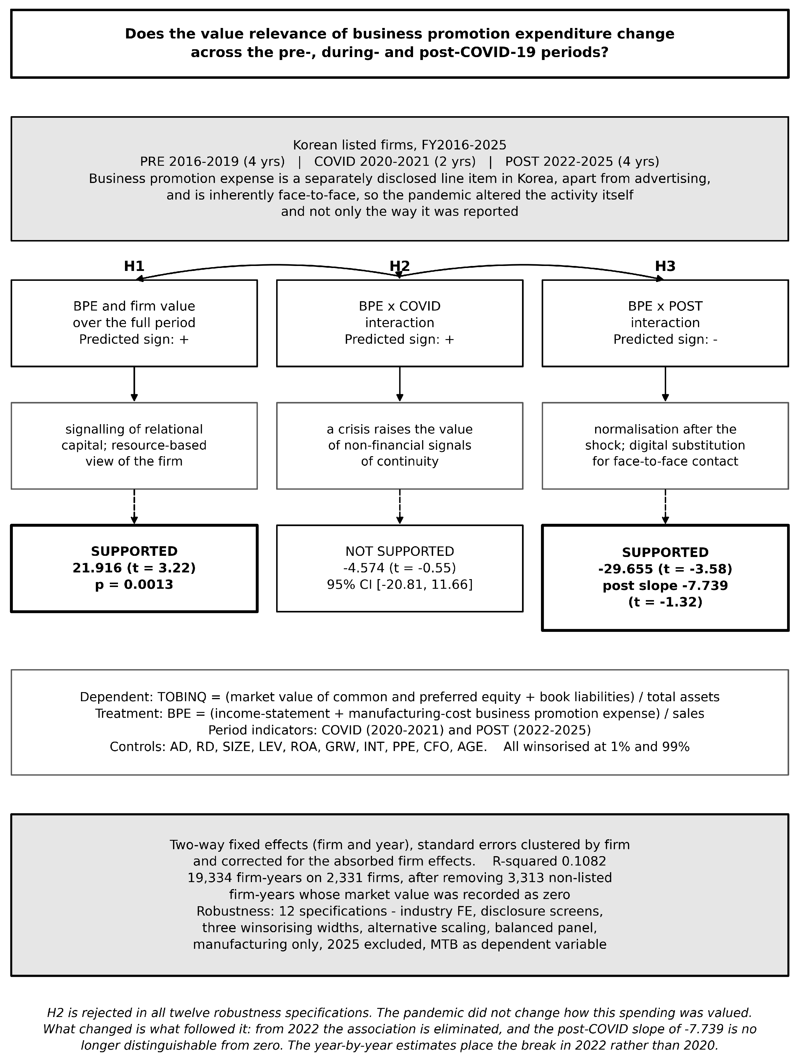
Figure 1.
Research structure: question, hypotheses, variables and identification.
4. Research Design
4.1. Model
The tests estimate
where COVID indicates the fiscal years 2020 and 2021 and POST indicates 2022 through 2025. The period main effects are absorbed by the year fixed effects and are not separately estimated.
TOBINQi,t = b0 + b1 BPEi,t + b2 BPEi,t × COVIDt + b3 BPEi,t × POSTt + Controlsi,t + firmi + yeart + ei,t
The specification is an interacted value relevance regression rather than a residual income model estimated directly. The choice follows the applied convention in this literature, which regresses a market-based measure on the accounting item of interest and a set of fundamentals rather than imposing the full structure of the valuation identity (Ohlson, 1995; Feltham and Ohlson, 1995; Barth, Beaver and Landsman, 2001). Nothing in the hypotheses requires the stronger structure, and imposing it would restrict the controls in ways that are hard to defend when the item under study is a single expensed outlay.
The coefficient b1 is the association between entertainment intensity and value in the pre-pandemic years and tests H1. The interactions b2 and b3 are differences relative to that benchmark and test H2 and H3, so that the association during the pandemic is b1 + b2 and the association after it is b1 + b3. Reporting these sums separately matters because a negative b3 is consistent both with a return to indifference and with active discounting, and only the sum distinguishes them; the two are reported as linear combinations in Panel B of Table 6.
A simpler design would split the sample into three periods and compare coefficients across subsamples. That is avoided here for two reasons. Subsample estimation discards the cross-period restriction on the control coefficients, so any difference in the entertainment slope is confounded with differences in how the controls operate; and it provides no direct test of whether the slopes differ, which the interaction terms supply. Where a design compares outcomes across periods, inference also has to contend with serial correlation within units, and comparing point estimates from separate regressions makes that harder rather than easier (Bertrand, Duflo and Mullainathan, 2004).
Firm fixed effects absorb the possibility that firms which entertain heavily differ persistently from those which do not in ways that also affect valuation, which is the first-order concern in a cross-section of this kind: industry, business model, customer concentration and managerial style are all plausible common causes and all are largely time-invariant over a decade. Identification therefore comes from changes within a firm over time. The alternative of controlling for the unobserved heterogeneity by including group averages or by adjusting the dependent variable is known to be biased, and the fixed effects estimator is the appropriate instrument where the heterogeneity is at the unit level (Gormley and Matsa, 2014).
In estimation the firm effects are absorbed by the within-firm transformation and the year effects enter as dummy variables, with 2025 as the base year. The year dummies are demeaned along with every other regressor, so that the coefficients are numerically identical to those from an estimation that includes 2,331 firm dummies and nine year dummies directly. The coefficients from this transformation were confirmed against a full least-squares dummy variable estimation before the results were taken as final, and agree to nine decimal places; in an unbalanced panel that equivalence does not hold if the year dummies are left untransformed.
Standard errors are clustered by firm. A firm’s residuals are correlated across the ten years it appears, and treating firm-years as independent overstates precision substantially in panels of this shape (Petersen, 2009). Clustering on the firm dimension addresses that correlation and, because the year effects are removed by dummies, the residual cross-sectional dependence that would motivate a second clustering dimension is largely absorbed (Cameron, Gelbach and Miller, 2011). Degrees of freedom are set by the number of clusters rather than the number of observations, which is the conservative choice with 2,331 firms. Standard errors are computed from the survey-design variance estimator of PROC SURVEYREG in SAS 9.4, with one adjustment. Because the firm effects are removed by the within transformation rather than entered as regressors, that procedure does not count them when it forms its finite-sample correction, and the standard errors it reports are accordingly too small by a factor of the square root of (N − k) over (N − k − (G − 1)), where k is the number of regressors in the transformed model and G the number of firms. The correction is 1.066 in the main specification. All standard errors, t-statistics and p-values reported in the paper incorporate it. The adjustment was verified by estimating the model both ways on subsamples small enough for the dummy-variable form to be feasible: the coefficients agree to nine decimal places and the ratio of the two standard errors matches the factor above to five decimal places in every case.
A remark on one control that is deliberately absent. The book-to-market ratio is a standard control in valuation regressions, but its denominator is market value of equity, which is also the numerator of Tobin’s Q. Including it induces a mechanical negative association that inflates explanatory power without reflecting anything economic; in this sample it carried a t-statistic of −24.9 and roughly doubled the reported R-squared while leaving the coefficients of interest essentially unchanged. It is excluded. Replacing it with the book value of equity scaled by assets is not an option either, since the balance sheet identity makes that variable the exact complement of leverage, with a sample correlation of −1.000.
4.2. Variables
The dependent variable is Tobin’s Q, computed as the market value of common and preferred equity plus the book value of liabilities, divided by total assets. This is the simple approximation rather than the replacement-cost construction of Lindenberg and Ross (1981), and the approximation tracks the theoretically preferred measure closely enough that the choice rarely alters inference (Chung and Pruitt, 1994; Perfect and Wiles, 1994). Because the numerator contains market value, the measure is also what makes the exclusion of the book-to-market ratio necessary, as explained below.
The test variable, BPE, is the sum of business promotion expense reported in the income statement and in the manufacturing cost statement, divided by sales. Taking only the income statement figure would understate spending at manufacturers, where a share of the cost attaches to production, and would do so in a way correlated with industry. Scaling by sales rather than by assets reflects that entertainment is an activity-related cost incurred in the course of selling; the asset-scaled alternative is reported in Table 10 and the difference it makes is discussed there.
The controls are chosen to close the channels through which entertainment intensity might appear to matter without doing so. Advertising and research intensity are constructed on the same two-statement basis and scaled by sales, so that BPE is not standing in for discretionary spending generally; both are priced in their own right (Erickson and Jacobson, 1992; Lev and Sougiannis, 1996; Joshi and Hanssens, 2010), and a firm that spends freely on one tends to spend freely on the others. Profitability and growth enter as return on assets computed on lagged assets and as sales growth, because a firm doing well can afford to entertain and is valued highly for reasons that have nothing to do with entertaining. Size, leverage, capital intensity and firm age are the standard conditioning set in valuation regressions of this kind. Intangible assets scaled by assets is included because recognised intangibles and unrecognised relational capital are substitutes in what they do for the firm, and because intangible intensity affects how much information reaches investors (Barth, Kasznik and McNichols, 2001). Operating cash flow over assets separates accrual-based profitability from realised cash generation. Table 2 gives the definition and computation of each.

Table 2.
Variable definitions.
| Variable | Type | Definition and computation |
| TOBINQ | Dependent | (Market value of common and preferred equity + book value of total liabilities) / total assets |
| BPE | Test | (Business promotion expense in the income statement + in the manufacturing cost statement) / sales |
| SPEND | Test | Indicator equal to one if BPE is greater than zero |
| COVID | Period | Indicator equal to one for fiscal years 2020 and 2021 |
| POST | Period | Indicator equal to one for fiscal years 2022 through 2025 |
| AD | Control | (Advertising expense in the income statement + in the manufacturing cost statement) / sales |
| RD | Control | (R&D expense in the income statement + in the manufacturing cost statement) / sales |
| SIZE | Control | Natural logarithm of total assets |
| LEV | Control | Total liabilities / total assets |
| ROA | Control | Operating income / lagged total assets |
| GRW | Control | (Sales − lagged sales) / lagged sales |
| INT | Control | Intangible assets / total assets |
| PPE | Control | (Tangible assets − land − construction in progress) / total assets |
| CFO | Control | Cash flow from operations / total assets |
| AGE | Control | Natural logarithm of (fiscal year − year of establishment) |
Notes: All items are from ValueSearch (NICE Information Service). Where an expense is reported in both the income statement and the manufacturing cost statement, the two figures are summed before scaling.
All continuous variables are winsorised at the first and ninety-ninth percentiles. Entertainment intensity has a long right tail, and in accounting samples a small number of influential observations can drive a reported coefficient entirely, so the treatment is not cosmetic (Leone, Minutti-Meza and Wasley, 2019). Winsorising rather than trimming retains the observation while limiting its leverage. Because the choice of cut-off is a researcher decision, three alternative widths are reported in Table 10, along with a specification that removes the upper tail outright.
4.3. Sample
Financial statement and market data are from ValueSearch, which draws on the audited filings of Korean listed companies. Four extracts were merged on the firm identifier: a general file carrying market value, balance sheet items, income statement items, advertising and business promotion expense; a cash flow file carrying sales and operating cash flow; a file carrying research and development expense and tangible assets from both the income statement and the manufacturing cost statement; and a file carrying ownership.
Table 1 reports the selection. The decade of firm-years for all listed companies gives 37,490 observations. Firms with a fiscal year ending other than in December are removed so that periods are comparable, and financial firms are removed because the valuation model does not apply to them. Observations without firm size or founding year, without positive assets, or without positive sales are dropped, the last because the ratio variables are undefined.
Table 1.
Sample selection.
| Selection step | Dropped | Remaining |
| Firm-year observations, Korean listed firms, FY2016–2025 | 37,490 | |
| Less: fiscal year end other than December | 9970 | 27,520 |
| Less: financial industry (KSIC section K) | 2730 | 24,790 |
| Less: missing firm size or year of establishment | 1190 | 23,600 |
| Less: total assets not positive | 637 | 22,963 |
| Less: sales not positive (ratio variables undefined) | 187 | 22,776 |
| Less: market value recorded as zero (pre-listing firm-years) | 3313 | 19,463 |
| Less: missing lagged assets or lagged sales | 129 | 19,334 |
| Final sample | 19,334 |
Notes: The population is all firms listed on the Korea Exchange with financial statement data in ValueSearch for fiscal years 2016 to 2025.
One further screen deserves comment because it is not routine and because omitting it materially changes the results. The database records a market value of zero for firm-years preceding a company’s listing. Those observations are not missing at random: they are concentrated in the early years of the sample, falling from 25.4 per cent of observations in 2016 to 0.3 per cent in 2025, and they carry a mechanically low Tobin’s Q because the numerator loses its equity component. Retaining them therefore embeds a spurious upward trend in measured firm value over exactly the horizon this study examines. They are excluded, which removes 3,313 firm-years. Requiring lagged assets and lagged sales for the return and growth controls removes a further 129. The final sample is 19,334 firm-years on 2,331 firms, unbalanced, with between one and ten observations per firm.
5. Results
5.1. Descriptive Statistics
Table 3 reports the distributions. Tobin’s Q averages 1.622 with a median of 1.167, so the mean is pulled up by a right tail even after winsorising. Business promotion expenditure averages 0.319 per cent of sales with a median of 0.117 per cent, which is small relative to advertising at 1.093 per cent and reflects that the account is a modest line item for most firms and a substantial one for few. Manufacturing accounts for 68.2 per cent of the sample.
Table 3.
Descriptive statistics.
| Variable | N | Mean | SD | Min | Q1 | Median | Q3 | Max |
| TOBINQ | 19,334 | 1.6223 | 1.419 | 0.4106 | 0.8512 | 1.1673 | 1.7957 | 9.3294 |
| BPE | 19,334 | 0.0032 | 0.0058 | 0.0 | 0.0002 | 0.0012 | 0.0035 | 0.0389 |
| AD | 19,334 | 0.0109 | 0.0288 | 0.0 | 0.0 | 0.0006 | 0.0063 | 0.1915 |
| RD | 19,334 | 0.0597 | 0.2556 | 0.0 | 0.0 | 0.0001 | 0.0282 | 2.2059 |
| SIZE | 19,334 | 25.9664 | 1.3319 | 23.4908 | 25.0522 | 25.7559 | 26.6458 | 30.5277 |
| LEV | 19,334 | 0.3653 | 0.2019 | 0.0315 | 0.1981 | 0.3551 | 0.5096 | 0.8871 |
| ROA | 19,334 | 0.0235 | 0.1004 | -0.3773 | -0.0081 | 0.027 | 0.0675 | 0.3292 |
| GRW | 19,334 | 0.0948 | 0.4241 | -0.6898 | -0.0867 | 0.0344 | 0.1739 | 2.6762 |
| INT | 19,334 | 0.0228 | 0.0409 | 0.0 | 0.0032 | 0.0085 | 0.0222 | 0.2589 |
| PPE | 19,334 | 0.1401 | 0.1218 | 0.001 | 0.0451 | 0.1077 | 0.2013 | 0.5718 |
| CFO | 19,334 | 0.0314 | 0.0929 | -0.3014 | -0.01 | 0.0368 | 0.0841 | 0.2643 |
| AGE | 19,334 | 3.1509 | 0.7292 | 0.6931 | 2.8332 | 3.2189 | 3.7136 | 4.2627 |
Notes: 19,334 firm-years on 2,331 firms. All variables winsorised at the first and ninety-ninth percentiles.
Table 4 splits the descriptive statistics by period. Average Tobin’s Q was 1.594 before the pandemic, 1.934 during it and 1.506 after, so the valuation environment differed sharply across the three windows; this is what the year fixed effects absorb. Average entertainment intensity fell from 0.308 per cent before to 0.275 per cent during the pandemic and then rose to 0.346 per cent after, so the aggregate spending series does not by itself explain what follows.
Table 4.
Descriptive statistics by period.
| index | Firm-years | Tobin’s Q | BPE | AD |
| Pre-COVID (2016–2019) | 6782 | 1.59432 | 0.00308 | 0.00964 |
| COVID (2020–2021) | 3868 | 1.93364 | 0.00275 | 0.01067 |
| Post-COVID (2022–2025) | 8684 | 1.50552 | 0.00346 | 0.01204 |
Notes: Means of winsorised variables.
Table 5 reports correlations, none of which suggests a collinearity problem among the controls.
Table 5.
Pearson correlations.
| TOBINQ | BPE | AD | RD | SIZE | LEV | ROA | GRW | INT | PPE | CFO | AGE | |
| TOBINQ | 1.0 | 0.21 | 0.15 | 0.35 | -0.23 | -0.04 | -0.15 | 0.14 | 0.14 | -0.04 | -0.16 | -0.24 |
| BPE | 0.21 | 1.0 | 0.19 | 0.38 | -0.31 | -0.05 | -0.34 | -0.04 | 0.08 | -0.1 | -0.29 | -0.11 |
| AD | 0.15 | 0.19 | 1.0 | 0.18 | -0.06 | -0.09 | -0.15 | 0.02 | 0.1 | -0.09 | -0.14 | -0.13 |
| RD | 0.35 | 0.38 | 0.18 | 1.0 | -0.16 | -0.06 | -0.43 | 0.07 | 0.02 | -0.02 | -0.35 | -0.16 |
| SIZE | -0.23 | -0.31 | -0.06 | -0.16 | 1.0 | 0.16 | 0.25 | -0.02 | -0.02 | 0.14 | 0.24 | 0.23 |
| LEV | -0.04 | -0.05 | -0.09 | -0.06 | 0.16 | 1.0 | -0.16 | 0.01 | 0.01 | 0.25 | -0.12 | 0.03 |
| ROA | -0.15 | -0.34 | -0.15 | -0.43 | 0.25 | -0.16 | 1.0 | 0.16 | -0.02 | 0.0 | 0.68 | 0.01 |
| GRW | 0.14 | -0.04 | 0.02 | 0.07 | -0.02 | 0.01 | 0.16 | 1.0 | 0.07 | -0.03 | 0.02 | -0.1 |
| INT | 0.14 | 0.08 | 0.1 | 0.02 | -0.02 | 0.01 | -0.02 | 0.07 | 1.0 | -0.05 | 0.02 | -0.11 |
| PPE | -0.04 | -0.1 | -0.09 | -0.02 | 0.14 | 0.25 | 0.0 | -0.03 | -0.05 | 1.0 | 0.12 | 0.01 |
| CFO | -0.16 | -0.29 | -0.14 | -0.35 | 0.24 | -0.12 | 0.68 | 0.02 | 0.02 | 0.12 | 1.0 | 0.04 |
| AGE | -0.24 | -0.11 | -0.13 | -0.16 | 0.23 | 0.03 | 0.01 | -0.1 | -0.11 | 0.01 | 0.04 | 1.0 |
Notes: Correlations among winsorised variables. Coefficients are reported to two decimal places.
5.2. Main Results
Table 6 reports the estimates. Column 1 includes only advertising, size and leverage as controls; column 2 is the specification described above.
Table 6.
Business promotion expenditure and firm value across the COVID-19 timeline.
| Variable | (1) | (2) |
| BPE | 18.766*** (6.971) | 21.916*** (6.797) |
| BPE × COVID | -4.574 (8.283) | -4.574 (8.277) |
| BPE × POST | -30.257*** (8.405) | -29.655*** (8.276) |
| AD | -1.184 (1.061) | -0.865 (1.071) |
| SIZE | -0.415*** (0.063) | -0.442*** (0.063) |
| LEV | 0.093 (0.135) | 0.220 (0.139) |
| ROA | 0.983*** (0.233) | |
| GRW | 0.073** (0.030) | |
| INT | -0.404 (0.738) | |
| RD | 0.259 (0.238) | |
| PPE | -0.546** (0.219) | |
| CFO | -0.089 (0.122) | |
| AGE | -0.116 (0.105) | |
| Firm fixed effects | Yes | Yes |
| Year fixed effects | Yes | Yes |
| Observations | 19,334 | 19,334 |
| Firms | 2,331 | 2,331 |
| R-squared | 0.0986 | 0.1082 |
Notes: Dependent variable is Tobin’s Q. Firm effects are absorbed by within-firm transformation; year effects enter as dummy variables with 2025 as the base year. Standard errors clustered by firm in parentheses. Standard errors incorporate the degrees-of-freedom correction described in Section 4.1 for the firm effects removed by the within transformation. , , * denote significance at the ten, five and one per cent levels.*.
In column 2 the coefficient on BPE is 21.916 with a standard error of 6.797 and a t-statistic of 3.22, so entertainment intensity was positively associated with firm value in the years before the pandemic and H1 is supported. The interaction with the COVID indicator is −4.574 with a standard error of 8.277, statistically indistinguishable from zero, and H2 is rejected. The interaction with the post-pandemic indicator is −29.655 with a standard error of 8.276 and a t-statistic of −3.58, and H3 is supported.
The magnitudes are easier to read as period slopes, reported at the foot of Table 6.
Table 6.
Panel B. Estimated BPE slope by period.
| Period | Combination | Estimate | Std. error | t | p |
| Pre-COVID (2016–2019) | b1 | 21.916 | 6.797 | 3.22 | 0.0013 |
| COVID (2020–2021) | b1 + b2 | 17.342 | 7.732 | 2.24 | 0.0250 |
| Post-COVID (2022–2025) | b1 + b3 | -7.739 | 5.865 | -1.32 | 0.1871 |
Notes: Linear combinations of the coefficients in Table 6 column 2. Standard errors are those of the linear combination, clustered by firm, and incorporate the degrees-of-freedom correction described inSection 4.1.
Before the pandemic the association was 21.916 with a t-statistic of 3.22; during it, 17.342 with a t-statistic of 2.24; after it, −7.739 with a t-statistic of −1.32 and a p-value of 0.187. A one standard deviation increase in entertainment intensity was associated with a Tobin’s Q higher by 0.127 before the pandemic, which is 7.8 per cent of the sample mean.
The post-pandemic slope is negative in point estimate but is not distinguishable from zero. What the data establish is that the association was eliminated: the change from the pre-pandemic benchmark is large and precisely estimated, while the level that remains is not. H3 predicted weakening and the point estimate goes past it, but the claim the evidence supports is elimination rather than reversal, and the paper is written on that basis.
The ninety-five per cent confidence interval on the COVID interaction runs from −20.81 to 11.66. Since the pre-pandemic association is 21.916, the interval excludes any effect that would have increased the association by more than about half, and excludes the doubling that a strong reading of the crisis-signalling argument would imply. The interval is wide enough that a modest effect in either direction cannot be dismissed, and the result is best described as a precise enough null to reject the hypothesis rather than as evidence of exact zero.
5.3. Timing
The three-period design imposes a structure, and a coefficient that differs between windows may reflect a trend rather than a break. Table 7 addresses this by estimating a separate slope for each year, and Figure 2 plots them.
Table 7.
Year-by-year BPE slope.
| Fiscal year | Period | BPE slope | Std. error | t | p |
| 2016 | Pre | 17.945 | 8.200 | 2.19 | 0.0287 |
| 2017 | Pre | 30.984 | 10.099 | 3.07 | 0.0022 |
| 2018 | Pre | 18.954 | 7.145 | 2.65 | 0.0080 |
| 2019 | Pre | 11.566 | 7.056 | 1.64 | 0.1013 |
| 2020 | COVID | 19.702 | 9.817 | 2.01 | 0.0449 |
| 2021 | COVID | 12.941 | 7.957 | 1.63 | 0.1040 |
| 2022 | Post | -1.672 | 7.060 | -0.24 | 0.8128 |
| 2023 | Post | -1.694 | 7.405 | -0.23 | 0.8191 |
| 2024 | Post | -8.062 | 6.228 | -1.29 | 0.1956 |
| 2025 | Post | -12.324 | 6.972 | -1.77 | 0.0773 |
Notes: Each row is a separate regression in which BPE is interacted with an indicator for that year. The reported slope is the sum of the BPE coefficient and the interaction. Standard errors are clustered by firm and incorporate the degrees-of-freedom correction described in Section 4.1.
The slope is positive in every year from 2016 through 2021: 17.95, 30.98, 18.95 and 11.57 in the pre-pandemic years, and 19.70 and 12.94 in the two pandemic years, with the 2019 and 2021 estimates not individually significant. It turns negative in 2022 at −1.67, remains negative in 2023 at −1.69, and reaches −8.06 in 2024 and −12.32 in 2025. Only the 2025 estimate is individually significant, and then only at the ten per cent level, so the year-by-year estimates establish the timing of the change rather than its precision; the pooled post-pandemic interaction is what carries statistical weight. The break occurs in 2022 rather than in 2020.
The periodisation therefore describes the data rather than creating the result, and the fact that the change coincides with the end of the pandemic rather than its onset is what the interpretation must accommodate.
5.4. Robustness
Table 10 reports twelve specifications.
Table 10.
Robustness.
| Specification | BPE | t | BPE × COVID | t | BPE × POST | t | N |
| (1) Main specification | 21.916 | 3.22 | -4.574 | -0.55 | -29.655 | -3.58 | 19,334 |
| (2) Industry and year fixed effects | 28.735 | 4.37 | -15.404 | -2.04 | -31.941 | -4.20 | 19,334 |
| (3) Winsorised at 0.5%/99.5% | 22.085 | 3.13 | -2.873 | -0.33 | -31.586 | -3.62 | 19,334 |
| (4) Winsorised at 2.5%/97.5% | 23.883 | 3.70 | -2.190 | -0.32 | -26.453 | -3.73 | 19,334 |
| (5) Winsorised at 5%/95% | 17.870 | 3.06 | 2.182 | 0.38 | -21.579 | -3.53 | 19,334 |
| (6) Firms with positive BPE only | 23.902 | 3.43 | -3.713 | -0.42 | -33.138 | -3.81 | 15,867 |
| (7) BPE scaled by total assets | 32.286 | 2.08 | 16.559 | 1.00 | -4.526 | -0.28 | 19,334 |
| (8) ln(1+BPE x 100) | 0.362 | 2.95 | -0.048 | -0.34 | -0.517 | -3.62 | 19,334 |
| (9) Balanced panel (10 years) | 14.884 | 2.00 | -13.249 | -1.45 | -27.805 | -2.89 | 15,260 |
| (10) Manufacturing firms only | 23.098 | 2.39 | -7.172 | -0.57 | -27.016 | -2.19 | 13,190 |
| (11) Excluding fiscal 2025 | 22.137 | 3.27 | -3.901 | -0.47 | -27.545 | -3.33 | 17,109 |
| (12) Dependent variable: MTB | 35.918 | 3.20 | -5.755 | -0.41 | -45.071 | -3.57 | 19,271 |
Notes: Each row is a separate regression with the full control set. Specification 2 replaces firm fixed effects with industry fixed effects. Specifications 3 to 5 vary the winsorising cut-offs. Standard errors are clustered by firm. All specifications except the second incorporate the degrees-of-freedom correction described in Section 4.1; the second does not require it, because its industry effects are entered as regressors rather than absorbed.
H2 is rejected in all twelve. In eleven the interaction is statistically indistinguishable from zero; in the twelfth, which replaces firm fixed effects with industry fixed effects, it is significantly negative at −15.404 with a t-statistic of −2.04. Since H2 predicted a positive coefficient, that specification rejects the hypothesis more sharply rather than reversing the conclusion. The post-pandemic decline holds in eleven of the twelve, with interaction coefficients between −21.579 and −45.071.
Two qualifications are reported rather than set aside. Scaling entertainment expenditure by total assets instead of sales leaves the post-pandemic interaction insignificant, at −4.526 with a t-statistic of −0.28. Sales is the more appropriate deflator for an activity-related cost, but the result does depend on that choice. Separately, the H1 coefficient is sensitive to the right tail: excluding the top five per cent of the entertainment intensity distribution leaves it statistically indistinguishable from zero, while the post-pandemic interaction becomes larger in absolute value. The pre-pandemic positive association is therefore driven substantially by heavy spenders, and the paper’s conclusions rest on H3 rather than on H1.
6. Additional Analyses
6.1. The Extensive and the Intensive Margin
A firm-year in which no business promotion expense appears is a firm-year in which the account does not exist, which is to say that the firm did not spend. Zero is a level of spending and not a gap in the record. That permits the decision to spend to be separated from the amount spent, and Table 9 does so.
Table 9.
The extensive and the intensive margin.
| Variable | (1) Extensive | (2) Intensive | (3) Both |
| SPEND | 0.007 (0.060) | -0.055 (0.061) | |
| SPEND × COVID | -0.043 (0.070) | -0.021 (0.073) | |
| SPEND × POST | 0.058 (0.072) | 0.189** (0.074) | |
| BPE | 23.902*** (6.962) | 23.349*** (6.959) | |
| BPE × COVID | -3.713 (8.761) | -4.176 (8.547) | |
| BPE × POST | -33.138*** (8.696) | -33.329*** (8.528) | |
| Controls, firm FE, year FE | Yes | Yes | Yes |
| Observations | 19,334 | 15,867 | 19,334 |
| Firms | 2,331 | 2,061 | 2,331 |
| R-squared | 0.1007 | 0.1012 | 0.1099 |
Notes: SPEND is an indicator for positive business promotion expenditure. Column 2 restricts the sample to firm-years with positive expenditure. Standard errors clustered by firm in parentheses. Standard errors incorporate the degrees-of-freedom correction described in Section 4.1 for the firm effects removed by the within transformation.
Entering only an indicator for positive spending, the coefficient is 0.007 with a t-statistic of 0.12 and neither interaction approaching significance. Whether a firm entertains at all is unrelated to its valuation, before, during or after the pandemic. Restricting the sample to firms that do spend and estimating on intensity alone reproduces the main pattern more strongly, at 23.902 before and −33.138 for the post-pandemic interaction, both significant at the one per cent level. Entering both margins together leaves intensity intact at 23.349 and −33.329.
What the market prices is the amount, not the act. This narrows the interpretation: an explanation resting on the mere presence or absence of entertainment activity cannot account for the findings, whereas one resting on the scale of spending can.
One coefficient in the combined specification runs against the grain and is reported for completeness. The interaction between the spending indicator and the post-pandemic period is 0.189 with a t-statistic of 2.55. Holding intensity constant, firms that spent something were valued more highly after the pandemic than firms that spent nothing. The coefficient is not significant when the indicator is entered alone, so it is not emphasised here.
6.2. The Disappearance of Spenders
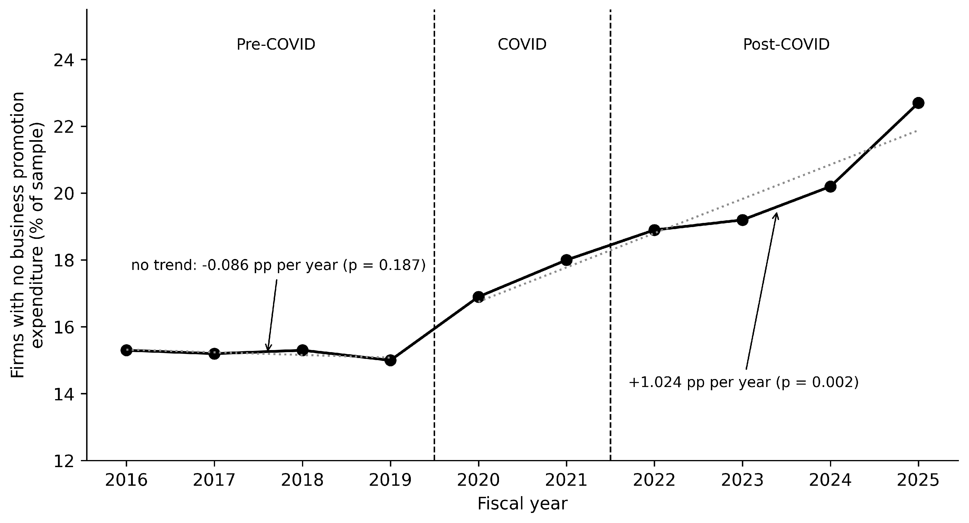
If the account measures activity rather than reporting practice, the share of firms with no entertainment expenditure is itself an observable series, and Table 8 and Figure 3 report it.
Table 8.
Firms reporting no business promotion expenditure.
| Fiscal year | Firm-years | No BPE (%) | Ceased spending (%) |
| 2016 | 1574 | 15.3 | |
| 2017 | 1648 | 15.2 | 2.2 |
| 2018 | 1741 | 15.3 | 2.3 |
| 2019 | 1819 | 15.0 | 1.6 |
| 2020 | 1888 | 16.9 | 3.3 |
| 2021 | 1980 | 18.0 | 2.9 |
| 2022 | 2061 | 18.9 | 2.7 |
| 2023 | 2147 | 19.2 | 1.9 |
| 2024 | 2251 | 20.2 | 2.2 |
| 2025 | 2225 | 22.7 | 3.6 |
Notes: The final column is the percentage of firms that reported expenditure in the previous year and none in the year shown; it is undefined for 2016.
The share is flat through the pre-pandemic years at 15.3, 15.2, 15.3 and 15.0 per cent; a trend fitted to those four years has a slope of −0.086 percentage points per year with a p-value of 0.187. From 2020 it rises every year, reaching 22.7 per cent in 2025, and a trend fitted from 2020 has a slope of 1.024 percentage points per year with a p-value of 0.002. The rate at which firms that spent in one year ceased spending in the next rose from an average of 2.02 per cent in the pre-pandemic years to 3.08 per cent during the pandemic, a difference significant at the one per cent level (t = 2.80, p = 0.005, unequal variances). It settled at 2.58 per cent after the pandemic, above the pre-pandemic rate but below the rate during it.
Korean firms did not merely spend less on entertainment during the pandemic; a growing number of them stopped altogether and did not resume.
The break in this series occurs in 2020, at the onset, whereas the break in valuation occurs in 2022. The behavioural change came first and the repricing followed, which is consistent with a market that reassessed the account only once the change proved durable.
6.3. Cross-Sectional Variation
Table 11 reports four splits, none of which is decisive, and all four are reported so that the pattern can be judged as a whole.
Table 11.
Cross-sectional variation.
| Partitioning variable M | BPE × M | t | BPE × COVID × M | t | BPE × POST × M | t | N |
| A. Sharp cut in BPE during COVID | -14.813 | -1.06 | -7.545 | -0.38 | -3.123 | -0.18 | 15,603 |
| B. Foreign ownership (continuous, standardised) | -27.457 | -2.24 | 23.307 | 2.02 | 19.552 | 2.16 | 19,334 |
| C. KOSPI listing | -19.050 | -1.94 | -2.265 | -0.16 | 15.413 | 1.17 | 19,334 |
| D. Firm size (continuous, standardised) | -23.340 | -2.24 | 10.289 | 0.67 | 17.948 | 1.14 | 19,334 |
Notes: Each row is a separate regression including BPE, its two period interactions, the partitioning variable interacted with each period, and the three triple interactions reported here. Standard errors are clustered by firm and incorporate the degrees-of-freedom correction described in Section 4.1.
Dividing firms by whether they cut entertainment spending sharply during the pandemic produces nothing: the triple interaction is −3.123 with a t-statistic of −0.18, and the other two interactions are equally uninformative. Whatever the market was responding to, it was not the firm’s adjustment behaviour during the shock.
Foreign ownership is the most promising of the four. Entered as a continuous firm-level measure, the interaction of entertainment intensity with foreign ownership is −27.457 with a t-statistic of −2.24, the triple interaction with the COVID period is 23.307 with a t-statistic of 2.02, and with the post-pandemic period 19.552 with a t-statistic of 2.16, all significant at the five per cent level. Read literally, the association and its disappearance are both concentrated in firms with little foreign ownership, and firms with substantial foreign ownership never priced the account at all. That reading fits the monitoring role that foreign institutional investors have been shown to play (Ferreira and Matos, 2008; Aggarwal, Erel, Ferreira and Matos, 2011).
The quartile estimates qualify it.
Table 12.
Estimates by foreign ownership quartile.
| Foreign ownership quartile | N | BPE | t | BPE × POST | t | Post-COVID slope |
| Q1 (lowest) | 4,840 | 36.255 | 3.16 | -49.900 | -3.61 | -13.645 |
| Q2 | 4,835 | 9.073 | 0.83 | -21.179 | -1.95 | -12.106 |
| Q3 | 4,834 | 20.466 | 1.35 | 4.998 | 0.34 | 25.464 |
| Q4 (highest) | 4,825 | -5.864 | -0.41 | -38.689 | -1.53 | -44.553 |
Notes: Firms are sorted into quartiles on their mean foreign ownership over the sample period. Each quartile is estimated separately with the full control set. Standard errors are clustered by firm and incorporate the degrees-of-freedom correction described in Section 4.1, computed within each quartile.
The post-pandemic slope is −13.645 in the lowest foreign ownership quartile and −12.106 in the second, but 25.464 in the third and −44.553 in the fourth. Only in the lowest quartile is the pre-pandemic level itself precisely estimated, at 36.255 with a t-statistic of 3.16. The relation is not monotonic in foreign ownership, so the significance of the continuous specification owes something to the linear functional form it imposes. The defensible statement is that the pricing of entertainment spending, and its disappearance, are concentrated among firms with the least foreign ownership, without a monotone gradient across the rest of the distribution.
Splitting by listing market gives a coefficient on the interaction of intensity with a KOSPI indicator of −19.050 with a t-statistic of −1.94, significant only at the ten per cent level, which points weakly to the association being a KOSDAQ phenomenon; but the triple interaction with the post-pandemic period is 15.413 with a t-statistic of 1.17 and is insignificant, so there is no evidence that the post-pandemic change differed by market. Splitting by firm size gives the same pattern: intensity mattered less at large firms, but the post-pandemic change did not differ by size.
Taken together these tests locate the phenomenon among smaller, domestically held firms without identifying the mechanism that produced it. That is a limitation of the study and is stated as one.
7. Conclusions
This paper asks whether the market’s valuation of business promotion expenditure changed around COVID-19, using ten years of Korean listed firms and a separately disclosed account that most jurisdictions do not report. Entertainment intensity was positively associated with Tobin’s Q before the pandemic. During the pandemic the association was unchanged. After the pandemic it disappeared, and the point estimates for the later years are negative.
The central finding is the one that was not expected. A crisis in which face-to-face contact became impossible did not change how the market valued spending on face-to-face contact. The change came afterwards, and the year-by-year estimates put it in 2022. Whatever the market learned, it did not learn it during the shock.
Two results support reading this as a durable change in practice rather than a temporary disturbance. The share of firms spending nothing on entertainment was flat before 2020 and has risen every year since, reaching 22.7 per cent in 2025, so the underlying activity contracted and did not recover. And the market prices the amount spent rather than the fact of spending, so the repricing concerns the scale of entertainment rather than its existence.
For research, the results caution against inferring the persistence of a shock’s effects from evidence gathered while the shock was still running. A study of this question ending in 2021 would have found nothing and concluded that the pandemic left the valuation of relational spending untouched, which was true and incomplete. For practice, the results suggest that entertainment budgets restored to their previous scale are not being read by investors as they were before 2020.
The study has limits. It documents an association without identifying a cause; there is no exogenous variation in entertainment spending, and the post-pandemic window contains other changes to the Korean economy that could correlate with entertainment intensity. The cross-sectional tests narrow the phenomenon to smaller and domestically held firms but do not establish the mechanism, and the foreign ownership result is not monotone across the distribution. The positive pre-pandemic association is sensitive to the upper tail of the spending distribution, and the post-pandemic result is not robust to scaling entertainment expenditure by assets rather than sales. Both qualifications are reported in Table 10 rather than relegated to a footnote.
Three directions follow. Whether the change reflects substitution of digital contact or a hardening of investor attitudes toward discretionary managerial spending could be separated with data on firms’ communication practices, which financial statements do not contain. Whether the pattern is Korean or general could be examined in Japan, where filings permit a comparable measure to be constructed. And whether the tax deductibility cap interacts with the valuation effect is a question the present design does not address.
Author Contributions
The author confirms sole responsibility for the following: study conception and design, data collection, analysis and interpretation of results, and manuscript preparation.
Funding
This research received no external funding.
Institutional Review Board Statement
Not applicable. The study uses firm-level financial statement and market data and does not involve human subjects or animals.
Informed Consent Statement
Not applicable.
Data Availability Statement
The financial statement and market data analysed in this study were obtained from ValueSearch (NICE Information Service) under a subscription licence and cannot be redistributed by the author. The variable construction code and the analysis programs that reproduce every table and figure are available from the author on request.
Acknowledgments
During the preparation of this manuscript the author used Claude Opus 5 (Anthropic), in August 2026, for the purposes of copy-editing the author’s own existing text, that is, correcting and refining the English wording and grammar and the formatting of the reference list and tables. The tool was used solely as an auxiliary aid to improve the efficiency of the work, and no research question, hypothesis, result, interpretation or conclusion was generated by it. The author designed the study, collected and verified the data, specified and ran all analyses, and prepared the manuscript. The author has reviewed and edited the output and takes full responsibility for the content of this publication.
Conflicts of Interest
The author declares no conflicts of interest.
References
- Adithipyangkul, P.; Alon, I.; Zhang, T. Executive perks: Compensation and corporate performance in China. Asia Pac. J. Manag. 2011, 28(2), 401–425. [Google Scholar] [CrossRef]
- Aggarwal, R.; Erel, I.; Ferreira, M.; Matos, P. Does governance travel around the world? Evidence from institutional investors. J. Financ. Econ. 2011, 100(1), 154–181. [Google Scholar] [CrossRef]
- Albuquerque, R.; Koskinen, Y.; Yang, S.; Zhang, C. Resiliency of environmental and social stocks: An analysis of the exogenous COVID-19 market crash. Rev. Corp. Financ. Stud. 2020, 9(3), 593–621. [Google Scholar] [CrossRef] [PubMed]
- Amir, E.; Lev, B. Value-relevance of nonfinancial information: The wireless communications industry. J. Account. Econ. 1996, 22(1–3), 3–30. [Google Scholar] [CrossRef]
- Barrero, J. M.; Bloom, N.; Davis, S. J. Why working from home will stick; (NBER Working Paper No. 28731); National Bureau of Economic Research, 2021. [Google Scholar] [CrossRef]
- Barth, M. E.; Beaver, W. H.; Landsman, W. R. The relevance of the value relevance literature for financial accounting standard setting: Another view. J. Account. Econ. 2001, 31(1–3), 77–104. [Google Scholar] [CrossRef]
- Barth, M. E.; Kasznik, R.; McNichols, M. F. Analyst coverage and intangible assets. J. Account. Res. 2001, 39(1), 1–34. [Google Scholar] [CrossRef]
- Bertrand, M.; Duflo, E.; Mullainathan, S. How much should we trust differences-in-differences estimates? Q. J. Econ. 2004, 119(1), 249–275. [Google Scholar] [CrossRef]
- Bloom, N.; Liang, J.; Roberts, J.; Ying, Z. J. Does working from home work? Evidence from a Chinese experiment. Q. J. Econ. 2015, 130(1), 165–218. [Google Scholar] [CrossRef]
- Cai, H.; Fang, H.; Xu, L. C. Eat, drink, firms, government: An investigation of corruption from the entertainment and travel costs of Chinese firms. J. Law. Econ. 2011, 54(1), 55–78. [Google Scholar] [CrossRef]
- Cameron, A. C.; Gelbach, J. B.; Miller, D. L. Robust inference with multiway clustering. J. Bus. Econ. Stat. 2011, 29(2), 238–249. [Google Scholar] [CrossRef]
- Chauvin, K. W.; Hirschey, M. Advertising, R&D expenditures and the market value of the firm. Financ. Manag. 1993, 22(4), 128–140. [Google Scholar] [CrossRef]
- Choudhury, P. R.; Foroughi, C.; Larson, B. Work-from-anywhere: The productivity effects of geographic flexibility. Strateg. Manag. J. 2021, 42(4), 655–683. [Google Scholar] [CrossRef]
- Chung, K. H.; Pruitt, S. W. A simple approximation of Tobin’s q. Financ. Manag. 1994, 23(3), 70–74. [Google Scholar] [CrossRef]
- Collins, D. W.; Maydew, E. L.; Weiss, I. S. Changes in the value-relevance of earnings and book values over the past forty years. J. Account. Econ. 1997, 24(1), 39–67. [Google Scholar] [CrossRef]
- Core, J. E.; Guay, W. R.; Van Buskirk, A. Market valuations in the New Economy: An investigation of what has changed. J. Account. Econ. 2003, 34(1–3), 43–67. [Google Scholar] [CrossRef]
- Dechow, P.; Ge, W.; Schrand, C. Understanding earnings quality: A review of the proxies, their determinants and their consequences. J. Account. Econ. 2010, 50(2–3), 344–401. [Google Scholar] [CrossRef]
- Ding, W.; Levine, R.; Lin, C.; Xie, W. Corporate immunity to the COVID-19 pandemic. J. Financ. Econ. 2021, 141(2), 802–830. [Google Scholar] [CrossRef] [PubMed]
- Dyer, J. H.; Singh, H. The relational view: Cooperative strategy and sources of interorganizational competitive advantage. Acad. Manag. Rev. 1998, 23(4), 660–679. [Google Scholar] [CrossRef] [PubMed]
- Erickson, G.; Jacobson, R. Gaining comparative advantage through discretionary expenditures: The returns to R&D and advertising. Manag. Sci. 1992, 38(9), 1264–1279. [Google Scholar] [CrossRef]
- Faccio, M. Politically connected firms. Am. Econ. Rev. 2006, 96(1), 369–386. [Google Scholar] [CrossRef]
- Fahlenbrach, R.; Rageth, K.; Stulz, R. M. How valuable is financial flexibility when revenue stops? Evidence from the COVID-19 crisis. Rev. Financ. Stud. 2021, 34(11), 5474–5521. [Google Scholar] [CrossRef]
- Feltham, G. A.; Ohlson, J. A. Valuation and clean surplus accounting for operating and financial activities. Contemp. Account. Res. 1995, 11(2), 689–731. [Google Scholar] [CrossRef]
- Ferreira, M. A.; Matos, P. The colors of investors’ money: The role of institutional investors around the world. J. Financ. Econ. 2008, 88(3), 499–533. [Google Scholar] [CrossRef]
- Francis, J.; Schipper, K. Have financial statements lost their relevance? J. Account. Res. 1999, 37(2), 319–352. [Google Scholar] [CrossRef]
- Gormley, T. A.; Matsa, D. A. Common errors: How to (and not to) control for unobserved heterogeneity. Rev. Financ. Stud. 2014, 27(2), 617–661. [Google Scholar] [CrossRef]
- Gul, F. A.; Cheng, L. T. W.; Leung, T. Y. Perks and the informativeness of stock prices in the Chinese market. J. Corp. Financ. 2011, 17(5), 1410–1429. [Google Scholar] [CrossRef]
- Jensen, M. C.; Meckling, W. H. Theory of the firm: Managerial behavior, agency costs and ownership structure. J. Financ. Econ. 1976, 3(4), 305–360. [Google Scholar] [CrossRef]
- Joshi, A.; Hanssens, D. M. The direct and indirect effects of advertising spending on firm value. J. Mark. 2010, 74(1), 20–33. [Google Scholar] [CrossRef]
- Khwaja, A. I.; Mian, A. Do lenders favor politically connected firms? Rent provision in an emerging financial market. Q. J. Econ. 2005, 120(4), 1371–1411. [Google Scholar] [CrossRef]
- Kothari, S. P. Capital markets research in accounting. J. Account. Econ. 2001, 31(1–3), 105–231. [Google Scholar] [CrossRef]
- Leone, A. J.; Minutti-Meza, M.; Wasley, C. E. Influential observations and inference in accounting research. Account. Rev. 2019, 94(6), 337–364. [Google Scholar] [CrossRef]
- Lev, B.; Sougiannis, T. The capitalization, amortization, and value-relevance of R&D. J. Account. Econ. 1996, 21(1), 107–138. [Google Scholar] [CrossRef]
- Lev, B.; Zarowin, P. The boundaries of financial reporting and how to extend them. J. Account. Res. 1999, 37(2), 353–385. [Google Scholar] [CrossRef]
- Li, H.; Meng, L.; Wang, Q.; Zhou, L.-A. Political connections, financing and firm performance: Evidence from Chinese private firms. J. Dev. Econ. 2008, 87(2), 283–299. [Google Scholar] [CrossRef]
- Lindenberg, E. B.; Ross, S. A. Tobin’s q ratio and industrial organization. J. Bus. 1981, 54(1), 1–32. [Google Scholar] [CrossRef] [PubMed]
- Ohlson, J. A. Earnings, book values, and dividends in equity valuation. Contemp. Account. Res. 1995, 11(2), 661–687. [Google Scholar] [CrossRef]
- Park, S. H.; Luo, Y. Guanxi and organizational dynamics: Organizational networking in Chinese firms. Strateg. Manag. J. 2001, 22(5), 455–477. [Google Scholar] [CrossRef]
- Perfect, S. B.; Wiles, K. W. Alternative constructions of Tobin’s q: An empirical comparison. J. Empir. Financ. 1994, 1(3–4), 313–341. [Google Scholar] [CrossRef]
- Petersen, M. A. Estimating standard errors in finance panel data sets: Comparing approaches. Rev. Financ. Stud. 2009, 22(1), 435–480. [Google Scholar] [CrossRef]
- Rajan, R. G.; Wulf, J. Are perks purely managerial excess? J. Financ. Econ. 2006, 79(1), 1–33. [Google Scholar] [CrossRef]
- Ramelli, S.; Wagner, A. F. Feverish stock price reactions to COVID-19. Rev. Corp. Financ. Stud. 2020, 9(3), 622–655. [Google Scholar] [CrossRef] [PubMed]
- Sougiannis, T. The accounting based valuation of corporate R&D. Account. Rev. 1994, 69(1), 44–68. [Google Scholar] [CrossRef]
- Srinivasan, S.; Hanssens, D. M. Marketing and firm value: Metrics, methods, findings, and future directions. J. Mark. Res. 2009, 46(3), 293–312. [Google Scholar] [CrossRef]
- Xin, K.; Pearce, J. L. Guanxi: Connections as substitutes for formal institutional support. Acad. Manag. J. 1996, 39(6), 1641–1658. [Google Scholar] [CrossRef] [PubMed]
- Yermack, D. Flights of fancy: Corporate jets, CEO perquisites, and inferior shareholder returns. J. Financ. Econ. 2006, 80(1), 211–242. [Google Scholar] [CrossRef]
Figure 2.
Year-by-year BPE slope with 95 per cent confidence intervals.
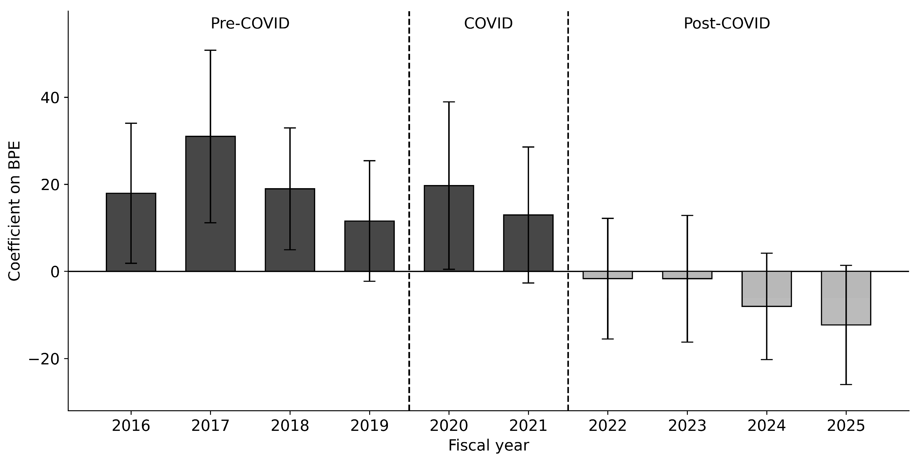
Figure 3.
Share of firms reporting no business promotion expenditure, 2016 to 2025.
Disclaimer/Publisher’s Note: The statements, opinions and data contained in all publications are solely those of the individual author(s) and contributor(s) and not of MDPI and/or the editor(s). MDPI and/or the editor(s) disclaim responsibility for any injury to people or property resulting from any ideas, methods, instructions or products referred to in the content. |
© 2026 by the author. Licensee MDPI, Basel, Switzerland. This article is an open access article distributed under the terms and conditions of the Creative Commons Attribution (CC BY) license.
Copyright: This open access article is published under a Creative Commons CC BY 4.0 license, which permit the free download, distribution, and reuse, provided that the author and preprint are cited in any reuse.