
Submitted:
20 August 2026
Posted:
21 August 2026
You are already at the latest version
Abstract
We propose a mathematical model for the structure of consciousness, and we do not treat the feeling itself. We build the model on a phase-augmented Recursive Heaviside Sequence Function, a cascade of nested smooth step functions in which each layer is one episodic memory carrying a time threshold \(\tau_i\), a sharpness \(s_i\), and an emotional phase \(\theta_i\). We propose that the objective of consciousness is survival, the drive to keep the remaining distance to a fixed endpoint short. Our central claim is that the partial derivatives of the objective functional \(E=|1-u_k|\) are thought, optimization, and decision, formed together at the present instant and without iteration. The state satisfies an advection equation whose right-hand side is a dummy source that the structure generates by itself, and substituting \(t=\tau_k\) removes the time variable and lowers the dimension by one. Each new experience adds an increment that decays exponentially with the delay, which we take to be the mechanism of forgetting and of childhood amnesia. In the second half, planning becomes a finite Taylor expansion about the present point, so proving a theorem, writing fiction, and telling a lie are one operation under different objectives. A perfect lie would need infinitely many partial derivatives, and no finite agent can supply them.
Keywords:
recursive Heaviside sequence function
; mathematical model of consciousness
; survival objective
; advection equation
; dimensional reduction
; thought as differentiation
; complex-phase memory model
1. Introduction
1.1. The Challenge of Mathematical Psychiatry
Psychiatry holds a special place among the medical fields. Its subject is the human mind, the disorders of the mind, and the treatment of those disorders. This subject resists the quantitative precision that we find in cardiology or in pharmacokinetics. Neuroscience has made remarkable progress for fifty years, but its effect on everyday psychiatric practice has been small [8]. The DSM and the ICD are the main systems in use. They classify disorders by clusters of symptoms, not by mechanisms. They lack the mechanistic and mathematical foundation that we need to predict precisely and to fit a treatment to one patient [9,23].
Computational psychiatry is one response to this gap [10]. Its premise is that the brain is a computational organ, and that the disorders arising from it therefore call for a computational framework. Two approaches have grown side by side. Data-driven methods apply machine learning and statistical modelling to large clinical data sets. Theory-driven methods build explicit mathematical models of the cognitive and neural processes [11]. This study belongs to the second group.
1.2. The Free-Energy Principle and Its Psychiatric Implications
The most influential framework in theoretical computational psychiatry is Karl Friston’s free-energy principle (FEP) [2,4]. The FEP proposes that biological agents, and the human brain among them, act to minimize the variational free energy. This quantity is an upper bound on the statistical surprise of the incoming sensory data [3]. Perception and action are both forms of free-energy minimization. The brain builds a generative model of the environment and keeps updating the model, to reduce the gap between the predicted signals and the observed signals [5,24]. This unifies perception and action under active inference [6], which other researchers have applied to psychiatric conditions [7].
Our framework shares with the FEP the view that optimization organizes mental activity. It differs in one respect. In the FEP, the minimization is asymptotic and it continues. Here, thought is an optimization that does not iterate. The mind completes it at a single present instant.
1.3. Reinforcement Learning and Computational Models of Depression
A parallel line of work applies reinforcement learning (RL) to mood disorders [9,12,13]. It models learning through a prediction-error signal that updates the value estimates [10,11]. As in the FEP, the optimization in RL is cumulative when enough time is available. We depart from both frameworks. We represent the optimization that a single present moment must complete at once, with no time to iterate.
1.4. The RHSF Framework: Background and Extension
We introduced the Recursive Heaviside Sequence Function in [1]. In that work, episodic memories are nested smooth step functions. Each layer is one memory episode. We index each layer by an event-time threshold and a sharpness , and, in the present extension, by a complex phase that carries the emotional colour of that memory. The earlier work [1] showed two things. First, the partial derivatives of the RHSF objective functional with respect to are the mathematical form of thought. Second, the layers tied to events in the distant past give derivatives that vanish. This explains childhood amnesia, and, when the number of layers goes to infinity, it explains how the mind blocks access to remote memories.
We develop this framework in three directions. First, we introduce the emotional phase and derive its derivatives. Second, we identify the objective functional with the drive to survive, that is, the drive to keep the distance to a fixed endpoint short, and we take the minimization of this functional to be thought itself. Third, we classify the partial derivatives of the objective on the parameter space as the units of thought, decision, and creation. The mind forms all of them at once at the present moment. We take up the clinical applications in a companion paper.
This places the present work in the theory-driven branch of computational psychiatry described above, and it is why that literature opens the paper. The theory-driven branch needs an explicit generative structure before it can model anything, and we offer the RHSF as one such structure. Its parameters , and stand for the event time, the salience, and the emotional valence. What we do not do here is use that structure clinically. By M3, the map from these parameters to clinical quantities has to be learned case by case, and we did not want to assert it on formal grounds alone.
1.5. Why Time, and Not Space
A reader may ask why we model the mind through time, attention, and mood, and never through a point in physical space. Our model has no spatial coordinate at all. We made this choice deliberately, and we state the reason plainly.
The feeling of a thought does not seem to sit anywhere in space. We look inside the brain — the anatomy, the cells, the synaptic molecules — and we find ions, voltages, and neurotransmitters. We never find the thought. Davies makes this point in God and the New Physics [14]. This is the gap that Chalmers called the hard problem of consciousness [15], and M1 places it outside our scope.
A reader may still hope that a complete molecule-by-molecule model of the brain in space would reproduce the mind. We feel that it would not, for four reasons.
First, we cannot count the variables. Such a model would track, at every point and every instant, the voltage, the current, and the concentration of every neurotransmitter and every modulator, together with all the sensory input and output. We cannot even list the coupled equations.
Second, even if we wrote the equations down, we could not be sure of solving them, not even numerically. Their size and their nonlinearity put a solution beyond any computing power that we can foresee.
Third, the object does not hold still. The brain is not a fixed circuit. It forms in the womb, and growth, experience, and education rebuild it across a whole life. Its architecture at any instant is what a developmental history has left behind, and that history belongs to one person. There is no fixed system to write down. We would have to rewrite the equations at every moment and for every person. That is to say, there is no single model to solve.
Fourth, and most important, even if we solved the equations, the answer would be numbers — fields of voltages and concentrations — and nothing in those numbers would be the mind. A number is not a thought until someone interprets it, and the interpretation is not in the number. The same value means different things to different people. One person reads grief where another reads relief. The dictionary that assigns the meaning is learned over a lifetime, and no two people share that lifetime. This is the interpretation gap, M3. The numbers are not the thought.
We say the same about the framework that follows here. Our own framework produces numbers. The , the , the , and the value of E are numbers and nothing else, and by M3 we do not hold the dictionary that reads them. We do not pretend otherwise.
We claim only this. The gap is narrower, and it is of another kind. A voltage at one point in one dendrite has no reading at all. We would have to find a further theory to give it one. A threshold is already the time of an event. A phase is already how that event felt. What is left to learn is which episode sits at which threshold in one person’s life. That is a table to fill in. It is not a theory that we still have to find.
For these reasons, we attempt no spatial reduction. We model the temporal and emotional shape of conscious episodes directly, through the time t, the event timing , the attention , and the mood , and we leave the spatial location out. We do not evade the physics. We recognize its limit. We ask how mental life unfolds in time, not where it sits in space.
1.6. Meta-Assumptions, Numerically Verified Properties, and Tool Choice of the Present Framework
The framework rests on five meta-assumptions, three numerically verified properties and one mathematical tool. We state them here and develop them in the rest of this section.
Meta-assumptions. We cannot test these directly. They say what the framework claims to be.
- M1
- (Qualia exclusion): This paper is not about qualia. We treat the structure and the behaviour of consciousness. We say nothing about how experience feels. By construction, the hard problem of consciousness [15] lies outside our scope.
- M2
- (Descriptive mapping): Our equations are not claims about how the brain computes. They express in mathematical form how consciousness behaves. We leave the neural mechanism open.
- M3
- (Interpretation gap): The framework produces numbers. It does not give the map from those numbers to clinical events and to experiences. We must learn that map case by case, the way a child learns that the sensation of red goes with the word “red”.
- M4
-
(Time-direction convention): Time flows from toward 0. We adopt this as a convention, and we do not derive it. Under this orientation, two things hold: the Heaviside causal structure of the RHSF, and the survival principle M5. The second one needs a fixed and finite endpoint 0, because only then is the distance to the end a definite quantity. We do not claim that the reverse orientation is impossible. We find that it does not suit these two requirements.Time runs from down toward 0, and it never reaches 0. The domain is the open interval , so thatholds everywhere in this paper. The endpoint 0 is fixed and finite, and it is approached and not attained. And we think only at the present:Thought is formed at that instant and nowhere else (T1). Outside it the cascade collapses, and there is nothing to read.The time-like variables, the observation time t and the thresholds , are physical times. We state every numerical illustration in this paper in these variables. They admit a logarithmic contraction,which maps onto and keeps the causal order, so that . We do not work in the contracted coordinate. A few passages below ask what the framework predicts under it, and the compression of remote event times is one of them. We mark those passages. We record (3) here once, so that the reader can follow and check them.
- M5
- (Survival as the objective): Consciousness carries an objective functional . When we minimize it, the residual goes to zero, that is, . Here 1 is not extinction. It is the run completed to the endpoint. Under M4, the present advances toward 0, so this is the tendency to keep the remaining distance to 0 short, that is, to remain in the world. The principle is well posed only because M4 makes the endpoint 0 fixed and finite. Then the distance to the end is a definite quantity, and the mind approaches it but never reaches it. This is a meta-hypothesis about the purpose of consciousness. It is not a theorem. We make it precise through E in §3. We should also say what it is not. M5 is a hypothesis about the form of the objective functional, that is, about which quantity the structure minimizes at each present instant. It is not an evolutionary claim. We do not argue that this form arose by selection, and nothing in the paper depends on such an argument. Where we use the word “instinct” below, we use it in the ordinary sense of an unlearned tendency, and not as an appeal to evolutionary history.
Numerically verified properties. We checked these by direct computation. We use them in what follows. We offer them as findings, not as proved results.
- T1
- (Primacy of the Present): Thought occurs only at the present moment ; cascade collapse renders the RHSF undefined elsewhere.
- T2
- (Time Direction): Time flows from to 0 in the RHSF coordinates; the reverse orientation is non-viable.
- T3
- (Thought = Decision = Creation): The optimization at the present moment uses all orders of partial derivative at once. Every partial derivative is a unit of thought, and every thought generates a new layer in .
We introduce the complex phase as a mathematical tool, not as a hypothesis. It carries the direction of an emotion separately from its intensity.
1.7. Scope and Hypothesis-Paper Character
By M1, we do not address the hard problem of consciousness [15], and we do not address the gap between a numerical output and a feeling [16]. These questions lie outside our scope, and they belong to a different kind of inquiry.
By M1 we also keep two things apart that are easy to run together. The paper treats the structural side of consciousness, and the survival objective of M5 belongs to that structural treatment: it names the quantity that the mind minimizes. It does not offer an evolutionary account of why that quantity, and we attempt none here.
This is a hypothesis paper. We offer one mathematical language for the structural side of psychiatric phenomena. Other researchers should test it, revise it, replace it, or add to it as the field learns more.
1.8. Organization of the Paper
The rest of §1 states the meta-hypotheses, the three numerical findings (T1, T2, and T3), and the complex-phase tool. It then defines the phase-augmented RHSF, derives the advection equation of the RHSF, and shows the drop in dimension that follows from the primacy of the present. It ends by identifying the dummy source as a residual that comes from the structure itself. In §2, we build up that dummy source stage by stage, under the convention that time flows from to 0. In §3, we introduce the survival objective and classify its derivatives as the units of thought. In the last section, we give our conclusions. We treat the clinical applications, the psychiatric consultation and the drug treatment, in a companion paper.
1.9. The Meta-Hypotheses in Detail
Three of the meta-hypotheses deserve emphasis. They govern how the reader should read this paper.
M1 (Qualia exclusion) comes first. Our outputs u, E, and are structural quantities. They do not represent qualia, and they do not generate qualia. A value does not tell us whether the state is the absence of consciousness, or equanimity, or death. Such questions belong to a different inquiry. A reader may object that does not tell us how the memory feels. That objection is about the scope, and it is not a refutation. We exclude the hard problem [15] by construction, not because we cannot reach it yet.
M2 (Descriptive mapping) says that the equations describe, and that they do not implement. The relation is the same as the relation between the wave equation and the seismic wave propagation in the earth. The equation describes the behaviour. The medium remains itself. The brain does whatever it does. We claim only that the behaviour of consciousness, when we write it as mathematics, takes the form that we develop here.
M3 (Interpretation gap) concerns the meaning. The framework produces numbers. The meaning of those numbers is not inside the framework. We do not know which life event goes with a threshold , and we do not know how a value of E relates to distress. We must learn this, the way a child learns that the sensation of red goes with the word “red”. This learned dictionary is not universal. Each person assembles it from a history that no one else has lived. Therefore, one observer may read a number one way and another observer may read the same number in another way. The same observer may read it differently at different times. The map from the number to the meaning is thus outside the framework, and it also depends in part on who reads it. We do not pretend that we hold this dictionary.
M1 fixes the scope, M2 fixes the status, and M3 fixes the reach of the meaning. We do not verify them in this paper. They are the position from which we write it. The reader should judge the framework by whether its predictions agree with the observations.
1.10. The Phase-Augmented RHSF
Under M1 to M3, we now define the object that we study. Shin [1] introduced the RHSF as a model of consciousness, in which episodic memories are nested smooth Heaviside (sigmoid) functions of the real thresholds . Here, we attach a complex phase at each threshold to carry the emotional colour. We give the full definition and the parameters in §1.16. We write the argument of the k-th layer as . The sign and the size of decide whether saturates near 0, saturates near 1, or sits in the transition region. The phase is our tool for separating the direction of an emotion from the intensity of that emotion (§1.14).
Our sharpest break from the existing computational accounts concerns the structure of time. Those accounts view consciousness as an inference system that is updated cumulatively along a continuous axis. We view consciousness as a sequence of instantaneous optimization events, and these events cannot be repeated. The three numerically verified properties below develop this view.
1.11. T1 (Primacy of the Present): the Cascade Collapses outside
Numerical finding 1 (Primacy of the Present)Human consciousness is defined only at the present moment. Thought arises at the threshold of the layer that is now active, that is, at when the layer k becomes active. Therefore, the RHSF u is meaningful and differentiable only for
At any other t, the nested structure goes throughcascade collapse. Then , and every partial derivative vanishes.
We verify T1 numerically in two cases.
Case A: Real-Valued Form ( for all k).
The RHSF reduces to the real chain . We take twelve layers with
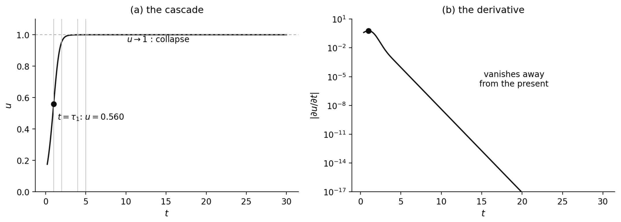
Case A1: the present moment . We compute the arguments from the inside outward. The inner layers () saturate at , and the outer two layers sit in the transition region of the smooth Heaviside function (, ; , ). Therefore, with , and the state is well defined and differentiable. The outer layers near the argument 0 are the ones that keep u from collapsing to 0 or to 1.
Case A2: the past time . Now the layer 5 gives (), the layer 4 gives (), and every outer argument is about . The whole structure collapses:
| all | ||
| (present) | nonzero, well-defined | |
| (past) | 0 |
Figure 1.
Cascade collapse away from the present (Case A, twelve layers, ). (a) At the present , the cascade sits in the transition region and . Away from the present, and the structure has collapsed. The vertical grey lines mark to . (b) The magnitude of . We compute it in 60-digit arithmetic, because double precision cancels below . It falls exponentially, and it is straight over seventeen decades. Thought is defined at the present and nowhere else.
Figure 1.
Cascade collapse away from the present (Case A, twelve layers, ). (a) At the present , the cascade sits in the transition region and . Away from the present, and the structure has collapsed. The vertical grey lines mark to . (b) The magnitude of . We compute it in 60-digit arithmetic, because double precision cancels below . It falls exponentially, and it is straight over seventeen decades. Thought is defined at the present and nowhere else.
Case B: Phase-Augmented Form ().
When , we have , so still controls the saturation. We take
and the same and . We obtain the following results.
- At , we obtain () and . The complex state is well defined.
- At , 50, and 1000, we obtain (within ) and .
The collapse pattern is the same as that of Case A. The phase does not save the function from the collapse outside the present moment.
Consequence: Time Travel into One’S Own Past Is Mathematically Impossible.
The reason is not causality. The reason is that the conscious self that would do the travelling is undefined at any moment other than . Remembering the past is not a return. It is a present-moment differentiation of the layers () that are nested inside .
1.12. T2 (Time Direction): Time Flows from to 0
Numerical finding 2 (Time direction>). In the RHSF framework, the distant past sits at and the present sits at . The contraction (3) of M4 preserves this orientation. The oldest episodic memory occupies the innermost layer , which carries the largest threshold. Each new episode adds a layer with a smaller threshold. The present is the outermost layer , which carries the smallest threshold. Time flows from toward 0, and it cannot cross 0.
This orientation is not a free choice. Under the reverse orientation, the framework collapses at every age.
Why the Reverse Orientation Does Not Work.
Suppose that we tried the standard physics convention, in which time runs from 0 to . The oldest memory would then sit at the smallest threshold, and the present would sit at the largest. At the present moment , the argument of the innermost layer would be with , which is large and negative. The smooth Heaviside saturates, so . By the cascade collapse mechanism of T1, the argument of every outer layer then reduces to . Every outer , so and every derivative goes to 0.
We check this numerically with four layers under the reversed convention, taking as the oldest layer and as the current age. Every , every , and . No present-moment consciousness is definable, and this holds at any age.
Why Works.
Under the correct orientation, the source contribution of the oldest memory involves . This sits near its maximum at birth, where , and it fades exponentially as the gap grows with age. The birth memory therefore starts near its maximum and fades to nothing by adulthood, which is exactly childhood amnesia. Two requirements thus force the orientation . The first is mathematical viability, because only this orientation gives a meaningful u at the present. The second is empirical correspondence, because only this orientation reproduces the fading of early memories.
1.13. T3 (Thought = Decision = Creation)
Numerical finding 3 (Thought = Decision = Creation)Thought at the present moment is an optimization of on the RHSF parameter space . It happens once, and it cannot be repeated. The next moment is already a different system on , with a new layer added, so the mind cannot iterate. Therefore, the optimization must use the partial derivatives of all orders at once. Two consequences follow.
- 1.
- Every partial derivative of E on Θ is a unit of conscious activity.
- 2.
- Every present-moment thought generates a new layer .
Thought, decision, and creation are three faces of one instantaneous event.
What the Derivatives Are for.
We state the point of T3 plainly before we give an example. A reader may read this section as a section about optimization technique. It is not.
We take the present state as given. It is one configuration , and everything that has happened has built it up. We differentiate E at that point, and we obtain a set of numbers: , , , and so on. Those numbers are the thought. They are not a means by which the mind does some separate thing that we call thinking. They are what thinking is at that instant. This is the first consequence in T3.
The numbers are also new. Not one of them is in the cascade before we differentiate. The function u holds them nowhere, just as is nowhere inside until we differentiate it. Differentiation does not read off what was already there. It makes something that was not there. This is why creation stands in T3 beside thought and decision.
The numbers do not evaporate either. The structure keeps them. They become the new outermost layer . This is the second consequence in T3, and it is the mechanism of §1.17. A thought is therefore not an event that happens and is over. It leaves a deposit, and that deposit is a layer. At the next instant, the mind differentiates a structure that now contains it.
When we read T3 in this way, the parallel with the artificial neural networks is structural, and it is not a metaphor. In both cases, a layer holds the values computed from the layer beneath. In both cases, the stack deepens as the computation proceeds. In both cases, what a given input yields depends on the values already deposited. The two differ in what fixes those values. In the neural network, the weights are fitted to the data. In the mind, the accumulated history of a life fixes them.
We note one consequence of this, because it is how the framework explains why people differ. Two people meet the same event, and they do not compute the same derivatives, because they differentiate at different points. Their , , and are what different histories have left behind. Different derivative values follow, and the two people deposit different layers. The gap widens, because tomorrow the mind differentiates a structure that includes the deposit of today. In this framework, individuality is not a separate faculty. It is the record of which derivatives a person has taken and stored. The same operation, run at different points, makes different people.
An Illustration for Readers Who Do Not Work in Optimization: The Three-Hump Camel Function.
We include the following example for one purpose. Readers who work in optimization may skip it. We wish to show a reader who has not seen such a landscape that having the derivatives is not the same as arriving at the best configuration. One can descend correctly and still settle in the wrong place. The example establishes nothing about T3, and we do not offer it as evidence for T3. It draws the shape of the terrain on which any descent occurs. We use a smooth function of two variables with several local minima, the three-hump camel function. It is a standard teaching example in nonlinear optimization and numerical analysis [25,26]:
This function has five critical points. There is a global minimum at with , there are two symmetric local minima at with , and there are two symmetric saddle points at with . Figure 2 shows one global basin, two shallower basins, and two saddle ridges between them. That is all that the figure is for.
First-Order Partial Derivatives.
A critical point of f satisfies , that is, both zero contours and pass through it. Figure 3 shows the two zero contours as thick lines. The zero set of is the straight line , and it crosses the quintic zero set of at five points. Three of these intersections are the local minima of f, and the other two are the saddle points.
Second-Order Partial Derivatives (Hessian).
The off-diagonal element of the Hessian matrix and are constant. Only varies. The Hessian matrix is positive definite at the three minima, that is, at the basins, and it is indefinite at the two saddle points, where . We show this in Figure 4.
Three Standard Iterative Methods.
Three standard methods find a minimum of f from a starting point [25,26]. The gradient descent method uses the first-order information only, and it is slow along a narrow valley. The Gauss–Newton method uses an approximate Hessian matrix , with the Levenberg–Marquardt damping when we need it. The full Newton method uses the exact Hessian matrix. It is the fastest one locally, and it is the most expensive one. All three methods iterate. They take a step, they recompute, and they take another step.
Figure 5 compares the three methods from the same starting point . We run each method for 30 iterations. The gradient descent method ends near the global minimum (), and the Gauss–Newton method reaches it almost exactly (). The full Newton method uses the complete Hessian matrix, but it is trapped in a local minimum (). The higher-order derivative information speeds up each step, but by itself it does not guarantee the global minimum.
Inversion Is Hard.
Even with the best iterative method, three difficulties run through all nonlinear inversion [25]. The first one is the non-uniqueness. Many parameter configurations give the same E. The second one is the local minimum. The iteration finds a minimum, and it is not necessarily the minimum we want. The third one is the failure to reach the global minimum. The iteration stalls on a saddle point or in a trapping basin. Figure 5(c) shows the second difficulty clearly. The full Newton method is the most sophisticated of the three, and it converges to a local minimum, not to the global one. These difficulties belong to the geometry of the objective function. They are not artifacts of the algorithm. In our framework, they take on a structural meaning. Thought is an instantaneous optimization on , and it can land on a local minimum, that is, on a stable configuration that is not the best one. We take this to be the mathematical face of cognitive rigidity and of some failures of insight. The optimization works. The landscape traps it. We treat the reshaping of such a landscape in the clinical companion paper.
Human Consciousness Does Not Iterate.
The three methods iterate. They take a step, they recompute, and they take another step. Conventional inversion works in this way, and the full-waveform inversion in geophysics is one example. It is very expensive. Consciousness is not this kind of algorithm. A car comes straight at a person. There is no time to compute a gradient, to take a step, and to recompute. The person must decide now. Consciousness uses whatever derivative information it has, all at once. It uses for the direction, the Hessian matrix when the first-order direction is not reliable, and the higher orders and the mixed orders for the harder cases. It does this instantaneously, and it does not iterate. Like the iterative methods, this one-shot optimization does not guarantee the global minimum. A person can be trapped in a local minimum too, in a fixed configuration that is not the best one. The three methods show what consciousness must do at a single stroke, and they show why it can fail.
A reader may object that dodging a car is a reflex, and that a reflex needs no appeal to consciousness at all. The objection would hold if the response were fixed. It is not fixed. The same person faces the same oncoming car, and the person dodges on one occasion and freezes on another. A fixed sensorimotor map cannot vary within one person whose wiring has not changed. A configuration that differs from moment to moment can vary. This is the point of the example. The response is the outcome of an evaluation on a parameter configuration, and different configurations give different decisions from the same input. A cat faces the same car and often runs into it. This is a further illustration, but it is a weaker one, because we can explain a difference between two species by the sensorimotor tuning, and we cannot explain a difference within one person in that way. The example is therefore not meant to show that a reflex proves consciousness. It is meant to show that the mind takes the decision on a configuration, and does not read it off a fixed map.
Derivatives Make New Forms.
Differentiation does not only contract. It also creates. We take and we differentiate it. We get , which is a line. We differentiate it again and we get , which is a constant. We differentiate it once more and we get 0. These are four objects of different kinds, and the act of differentiation made each one. In our framework, optimization, decision, and creation are one. Every partial derivative is at once an instrument of optimization, a unit of decision, and a new object made from the structure that was there before.
The Full Local Taylor Expansion Is Available at Once.
For an instantaneous decision, consciousness holds the complete local structure of E at the present point. It holds the first-order for the direction, the second-order Hessian matrix H for the reliability, and the higher orders and the mixed orders for the multifaceted judgment and the coupling. It holds all of them at once. Thought is not a simple gradient descent.
Two remarks fix the status of this statement.
First, the availability is not in question. The smooth cascade is in its parameters. Every partial derivative of every order therefore exists at the present point. Some process does not make them one after another, and no such process can run out of time.
Second, sequential use is not merely expensive. It is not available at all. By T1 and T3, the next instant is a different system on a larger parameter space. There is no second evaluation at the same point, and the mind cannot put a higher order off to such an evaluation. If the orders beyond the first enter the decision at all, they enter at that one evaluation.
One thing does remain open. We do not know how many orders a given agent brings to bear. This is a question of capacity, not of existence, and we offer it as a hypothesis. We take it up in §4, as the limit on how many mixed terms the mind can hold apart at once.
The camel example proves none of this, and we do not offer it as a proof. Its role is narrower. It shows that a single evaluation fixes a descent direction with no iteration. It also shows that even a method carrying the full Hessian matrix can be drawn into the wrong basin. One-shot optimization therefore gives no guarantee of the global minimum, however much derivative information it uses.
Difference from Existing Frameworks.
The FEP treats an asymptotic process that minimizes the free energy. RL integrates the prediction error cumulatively. In both frameworks, the optimization is cumulative when enough time is available. Here, thought does not iterate. All the orders appear together, at one point event.
1.14. Supplement: The Role of the Complex Phase — Why ?
We attach a complex phase to each threshold. We do this not for convenience. We need it to represent emotion at all.
Separation of Amplitude and Phase.
A single real variable can express only the intensity of an emotion. Strong sadness and strong joy come out as the same strength, and we lose the difference between them. We want three things. Sadness and joy should be different emotions, two emotions should be able to occur together, and one emotion should be able to pass continuously into another. For these three things, we need a direction as well as an intensity.
The complex phase gives us this. The phase carries the qualitative direction, that is, the valence. The amplitude , or the salience through , carries the intensity. By Euler’s formula, we write
Two people go through the same objective event. They share the real part, that is, when the event happened, but they may differ in the imaginary part, that is, how the event felt.
Why We Use a Modular Phase on .
The two phases and are the same. This gives us three properties that no real label can carry.
- 1.
- Continuous rotation. The passage from good to neutral to bad to neutral and back to good is a trajectory on . On the real axis, we cannot express this cyclic transition without a discontinuity.
- 2.
- The opposite emotion is not a sign reversal. In the clinic, the opposite of joy may be anhedonia, and the opposite of sadness may be anger. In the phase space, the opposite is a rotation by . The geometric opposite need not match the clinical one.
- 3.
- Phase interference. For the coupled layers, expresses the pattern. The coinciding phases amplify each other, and the phases that are apart cancel each other. This is the basis for ambivalence.
The Conservative Restriction .
We develop the framework under , so that and the real part dominates. We do this for two reasons. First, the mathematics stays tractable, because every derivative has a clear asymptotic form. Second, we are conservative. When we let the time outweigh the emotion, we say that for a typical memory, when it happened counts for more than how it felt. Strong trauma is an obvious counterexample.
Future Extension to .
We expect that the full circle will model two more cases.
(1) Trauma. For , the real part becomes negative or near zero. These are the memories in which how the event felt dominates over when it occurred. When a patient relives a trauma as if it were happening now, the real part has weakened.
(2) Bipolar disorder. We propose two mechanisms, and both agree with T1. In the first mechanism, each new episode forms a layer, and the phase of that layer alternates between positive and negative. The layers with inconsistent phases accumulate, and they produce a chronic mood instability. In the second mechanism, an abrupt mood change is a fresh layer with a very large and a that differs markedly from the existing phases. Because is near the present, dominates , and the mood switches instantaneously.
The of the future layers may enter a stable phase or an unstable one. We take up in the companion paper how an intervention might steer them toward stability.
1.15. Summary: Five Meta-Hypotheses, Three Numerical Findings, One Tool
The framework spine:
-
Meta-hypotheses (not directly testable):
- –
- M1 (Qualia exclusion): the paper is not about qualia; the hard problem of consciousness lies outside the framework’s scope by construction.
- –
- M2 (Descriptive mapping): equations describe consciousness mathematically, not how the brain implements it.
- –
- M3 (Interpretation gap): numerical output and clinical meaning must be linked through a learned dictionary, case by case.
- –
- M4 (Time-direction convention): time is taken to flow from toward 0. This is adopted as a convention and is not derived.
- –
- M5 (Survival as the objective): consciousness carries the objective functional , whose minimization drives the residual to zero, that is, . This is a hypothesis about the form of the objective, not an account of how that form arose.
-
Numerically verified properties (checked by direct computation, not proved):
- –
- T1 (Primacy of the Present): cascade collapse outside shows the RHSF is defined only at the present moment.
- –
- T2 (Time Direction): time flows from to 0 in RHSF coordinates; the reverse orientation is non-viable.
- –
- T3 (Thought = Decision = Creation): present-moment optimization requires all orders of partial derivative at once; every derivative is a unit of thought, and every thought creates a new layer.
- Mathematical tool: complex phase separates qualitative direction (valence) from intensity.
From this point onward, we use T1, T2, and T3 as working assumptions. They are numerical findings, and they are not theorems. We offer no proof for them, and we ask the reader to treat them as findings. The rest of the paper develops their mathematical consequences. These are the advection equation and the dimensional reduction, which we treat later in §1, the self-generative dummy source and the mechanism of forgetting, which we treat in §2, and the survival objective whose differentiation is thought, which we treat in §3.
1.16. Definition of the Phase-Augmented RHSF
We follow [1] and state the recursive Heaviside structure formally. We then introduce the present extension, which is the emotional phase factor at each threshold . This gives the phase-augmented RHSF, and we write it as a function of the time t:
The smooth Heaviside function and its derivative, which is the delta sequence, are
The parameters are the following.
- is the event-time threshold, that is, the marker of the episodic memory, with .
- is the salience, that is, the interest or the sensitivity, of the i-th layer. A larger widens the transition and slows the forgetting (Remark 1). The sharpness of the transition is proportional to .
- is the emotional phase. For the moment, we treat it under (see §1.14).
By Euler’s formula, we write
The real part governs when the k-th transition occurs, and the imaginary part carries the emotional colour of that transition. Under , we have , so the temporal meaning dominates. Figure 6 shows the multi-layer structure at representative parameters.
Remark 1
(Why s divides rather than multiplies: salience and the direction of forgetting). The standard sigmoid function of machine learning, , has a fixed transition width, and its derivative is . The RHSF places s in the exponent as , so that and
We do not place s in thedenominatoras an arbitrary scaling. This choice encodes thesalience, that is, the interest or the sensitivity, in the correct direction. The peak height of the delta sequence is about and its width is about s, so that the area is unity, as a delta sequence requires. The forgetting rate of Eq. (22) is proportional to . Two limits make the meaning concrete.
- High salience (large s).The decay rate is proportional to , so it is small. The contribution of a layer therefore survives over a large temporal gap . That is,we remember a memory of high interest for a long time.
- Vanishing salience (). stiffens into a true Heaviside step, and its derivative becomes a sharp spike. The spike is present at the instant , but it is extinguished at any earlier moment, because explosively for . That is,a memory that we pass over without interest exists only for a moment, and it becomes inaccessible at once.
Suppose that smultipliedthe argument instead, that is, . Then the correspondence would invert. A large s would give fast forgetting and a small s would give slow forgetting, and this contradicts the meaning of the salience. We therefore place s in the denominator, because the interest must prolong the memory and must not shorten it.
Remark 2
(The present moment, prediction, and thought). The cascade (7) is a function of t, but the experience is real only up to the present. As long as we add no new layer , (7) extends beyond the present and yields a prediction. Every threshold was itself once the present moment, so we may legitimately write . Present thought is the evaluation at , together with the partial derivatives of all orders at that point. It is at once thought, decision, and optimization (T3).
Remark 3
(Modification from [1]). The original RHSF uses only the real-valued . The present extension replaces each by , and this introduces a one-parameter family of emotional deviation at each layer. When we set for all k, we recover the original framework.
Remark 4
(Direction of time). Time flows from toward 0 (M4). The thresholds are physical times, and the contraction (3) of M4 keeps their order. Under the contraction, the semi-infinite axis is compressed into a bounded interval, and maps to . Either way, we have
and a larger is a more distant past. The innermost layer is the oldest episode, and the outermost layer is the present.
Remark 5
(Scale symmetry). The cascade (7) does not change under
applied to every layer at once, because depends on x and s only through .
We do not know where in the universe we stand, and we do not know which stretch of time we occupy. The framework says the same. Only the ratios and carry meaning, and the absolute value of a threshold is not a quantity here. This is why the dating of a remote event is lost in Remark 8, and why it goes altogether in the limit of Remark 10.
Remark 6
(Connection to the Heaviside causal form). We do not use by accident. We can write the causal solution of a linear evolution equation in the universal form , which is the product of a smooth kernel and a Heaviside function shifted by a positive infinitesimal. We do not impose the causality from outside. It is built into the solution itself. This matches the time-direction convention of the RHSF. Both say that what lies before the present does not exist. The first one says it as physical causality, and the second one says it as the restriction of the domain of conscious thought. T1 and the dimensional reduction of §1.18 express this universal Heaviside structure in the domain of consciousness.
The interval of integration: why there is no room
Suppose that the interval of integration is given as a window,
But in this framework we think only at the present, so we must set . When we do that, we obtain
This holds at every layer. The Heaviside function reads only the sign of its argument, and it does not read the size. Therefore whether is 10 or , and the two terms cancel either way. We checked this across the whole cascade. At the present, every window is zero. A separation exists and yet no window opens. The measure is not defined, and there is no room to integrate.
What this means. Suppose that the were marked on a time axis that is already in place. Then there would be a window of width , and the measure would be . A Fourier transform, or any other integral transform, would then be possible. This is not the case. No window opens, and this means that the do not lie side by side on one time axis. They are of a different dimension. They do not occupy a different space. They hide inside the time axis, like the rings of a tree, or like a Russian doll. Each new present winds one more layer, and that layer is a new dimension. Therefore the ordering condition
is not a restriction on a single axis. It is the condition that separates the time dimensions.
The hypothesis carries us this far. We must add one thing honestly. The definition of differs from author to author. The calculation above took . With , we obtain , and with , we obtain . The conclusion therefore depends on the definition. We have not settled that definition in this paper, and we leave it open.
1.17. The Natural Growth of Layers in the RHSF
One fundamental property of the RHSF is that the number of layers is not fixed. It grows naturally as new episodes occur. Every external stimulus, every recollection, every spontaneous thought, and every dream fragment adds a new layer to the existing structure, with a characteristic time delay.
Suppose that the current inner cascade is
which is a function of the parameters of the inner layers, that is, the older ones. When a new layer k is activated on the outside, we obtain
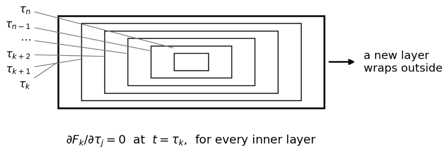
Each new layer wraps around the existing structure from the outside, that is, from the side of the present. The older layers remain as the inner block , and the most recent event becomes the new outermost layer. In the time order of the framework, , the inner layers carry the larger thresholds, which are the older ones, and the outer layers carry the smaller thresholds, which are the more recent ones.
Figure 7.
A new layer wraps on the outside. The innermost box is the oldest episode , and the outermost box is the present . Each new experience adds a box around the existing structure, and it never adds one inside. Therefore the information passes from the inside outward only. When we evaluate at the present, the partial derivative with respect to every inner threshold is 0. There is no direction along which the outside could reach an inner layer.
Figure 7.
A new layer wraps on the outside. The innermost box is the oldest episode , and the outermost box is the present . Each new experience adds a box around the existing structure, and it never adds one inside. Therefore the information passes from the inside outward only. When we evaluate at the present, the partial derivative with respect to every inner threshold is 0. There is no direction along which the outside could reach an inner layer.
The new layer does not arise from a force that we impose from the outside. It arises as a self-generated residual. The existing structure produces the differential responses
and these responses play the role of the source term that drives the formation of the new layer. The mind is therefore a variable-dimension self-feedback system, and its recursive depth grows through the lived experience. This holds whether the source is external, such as the sensory input, the conversation, or the consultation, or internal, such as the recollection, the rumination, or the dream. This is the mathematical expression of the corollary of T3, that every thought generates a new layer. Each new layer condenses, into a new encoding, the residual responses that the existing structure itself has generated.
The mind will think the future, but it has not thought it yet. The future layers correspond to the Heaviside functions that are not yet activated. They are absent from the present structure, so they contribute nothing to . These are direct consequences of T1, and they determine how we transform the advection equation below.
1.18. The Advection Equation and Dimensional Reduction
In this subsection, we introduce the advection equation that the phase-augmented RHSF satisfies, and we state the dimensional reduction that follows from T1.
The Original Advection Equation.
The phase-augmented RHSF u is at first a function on the -dimensional variable space , and it satisfies
The left-hand side is the sum of the first-order derivatives in all the time variables and event-time variables. The right-hand side is the dummy source S.
Applying T1.
By T1, thought occurs only at . Under this substitution, u no longer has an independent variable t. We write
and therefore
In Eq. (18), the term does not disappear. It becomes explicitly zero. The advection equation reduces to a reduced source equation on a variable space of one lower dimension:
Meaning.
The event-time dimensions absorb the time dimension:
| The original variable space | : | |
| The reduced space after T1 | : |
This is the precise mathematical meaning of the statement in T1 that thought occurs only at the present.
The Case .
In most of the analysis, we take , that is, the most recent layer is the present. The reduced equation becomes
The general case appears in the stage analysis of §2. Stage n corresponds to , and Stage corresponds to .
Note on Sign Conventions and Time Direction.
The advection equation above uses the convention in which t flows from toward 0. We state this convention in the remark on the time direction in §1.16. We build the RHSF by recursive nesting, so we apply the chain rule repeatedly against this reversed time direction. This produces the parity factors in front of the term at the stage k, and we give the explicit formulas in §2. This follows directly from the time-direction convention together with the nested differentiation. After we apply T1, all the terms vanish. The sign structure of §2 secures two properties that define the framework. The first one is the causality, that is, each in the limit that closes the residual. The second one is the exponential suppression of with the cumulative time delay, which is the mathematical mechanism of forgetting (§2.4).
All Thought Is Present Thought.
We must set aside one common confusion. People often fail to distinguish thinking in the future from designing the future, and they likewise fail to distinguish thinking in the past from recalling the past. A reader may suppose that planning ahead is thought that takes place at a future time. It is not. We design the future now, at the present instant. We form the derivatives , , and so on, of the existing structure, which is the record of the past experience, and we project from them. A past thought, in the same way, was made at what was then its own present. Thought never occurs at any time other than the present . This is why t is not an independent variable. We identify it with the present threshold, and the dimension drops accordingly. The reduction is not a technical convenience. It is the mathematical form of the fact that consciousness thinks only in the present.
1.19. Meaning of the Advection Equation: Average Steepest Descent and the Mechanism of Forgetting
Eq. (21) is not only a formal reduction. Three aspects deserve emphasis.
Aspect 1: The Average Steepest Descent (the Real Case).
When all , the cascade is real, and the left-hand side equals exactly, because with no mood. This is the summed steepest-descent direction of E. It is the natural direction in which consciousness moves, and the first-order information in all the parameters appears at once (T3). In the general complex case, where , we cannot read the equation literally as a descent direction. That reading is valid only for .
Aspect 2: The State of Complete Optimization.
We consider the cascade without the phase,
in the sharp limit . The delta sequence vanishes wherever the activation argument is far from the front, that is, where . We evaluate this at the present instant under the -shift with . This shift keeps the present off the activation front, and it avoids the divergence of on the front. Every first-order derivative then vanishes, and we obtain . This is a state of complete optimization. There is no dummy source and no force, and every derivative vanishes at once. That is, by the corollary of T3, every thought vanishes at once. This state corresponds to the cessation of thought, that is, to the asymptotic state in which the residual has closed (see §3.1). The condition has three parts: the zero phase , the sharp limit , and the evaluation off the front through the -shift. The phase alone does not suffice. In the general case with the phase, where , we obtain . Thought then occurs, but it occurs as a stationary residual, and the intensity of that residual is small and fades quickly.
Aspect 3: The Mathematical Mechanism of Forgetting.
At the present instant , the activation argument of the oldest layer takes the form , and the corresponding delta-sequence term is
The threshold is the oldest one, that is, the innermost one, and . Therefore the difference is a large negative number for a remote memory. Then , the denominator tends to 1, and
This is an exponential decay with the gap . The more distant the episode is, the faster its contribution vanishes. This is the mathematical basis of childhood amnesia, and the salience s sets the rate. Forgetting is therefore a natural decay that the RHSF structure produces. The weakening of sets the differential rate according to the interest. When we read the same result in the contracted coordinate (3), the transformation adds a uniform decay as the time passes. The account of childhood amnesia through the complementary processes [17] reaches a structurally similar conclusion from the empirical side.
Remark 7
(Combined effect). The differential decay is the mechanism in physical time. It is the amplitude of , and it acts layer by layer according to the interest. When we read the result in the contracted coordinate (3), a uniform temporal compression acts on all the layers alike, and it is superposed on the differential decay. The two together form the full memory-decay mechanism. This mechanism plays out on the static present-moment structure (T1) at the instant of optimization (T3).
Read in physical time through the contraction (3), the leading term of falls as
This is the shape of the forgetting curve that has been measured since Ebbinghaus, and we take it as a simple approximation and nothing more. It says that recent episodes weigh more than remote ones, and that a larger salience flattens the fall. We do not claim the exponent to any stated accuracy. The base a need not be constant (Remark 9), and s is not observed.
Remark 8
(Loss of chronological resolution: why the dating of a remote memory is uncertain by its nature). The logarithmic transformation compresses the amplitude of a memory through , and it also compresses thedistinguishability of the event times themselves. These are two different things. The base of the transformation grows with age, because each successive present carries a larger a. Therefore the transformed coordinates of consecutive remote events collapse toward one another. We reason in this paragraph in the contracted coordinate of (3). We take and a base that advances with the present, one unit for each five years, so that for . We then obtain
A five-year physical separation between a memory fifteen years past and one twenty years past therefore maps to a transformed gap of only . The successive gaps for the events at 25, 30, and 35 years shrink further, to , , and , and a recent pair, one year against two years, is separated by about at the base that the rule assigns to that age. The slope falls twice as fast when and a grow together, so the distant events pile up at nearly the same coordinate. The spacing drops below the resolution at which we can tell two coordinates apart. The events then becometemporally indistinguishable. The structure keeps the fact that they occurred, but it does not keepwhenthey occurred, or in what order.
This separation is a documented feature of human memory, and it is not a peculiarity of the model. On one side is the content and the vividness of a memory, and on the other side is its temporal location. The dating of an event is not an intrinsic part of its memory trace. It is a separate reconstructive process [18,19], so that the recollective vividness and the confident dating dissociate [20]. The accuracy of the temporal order and of the dating declines as events recede into the past, even when we still recognize the events themselves. In the present framework, this familiar pattern is the direct signature of the logarithmic contraction. The amplitude decay governshow stronglya memory surfaces, and the chronological compression governswhether we can locate its date at all.
Remark 9
(Cue-driven reactivation: the latency and the sudden return of a memory). The accessibility in the framework is not a quantity that only decays. It can alsorevive. The contribution of an inner layer k, that is, an older layer, to present thought enters through its delta sequence , where the activation argument is
The outer layers gate this argument through the factor . The function is bell-shaped. It is maximal at the front , and it is exponentially small for . Therefore a layer whose argument sits far from the front islatent. It is present, but it does not surface, and . A later experience then wraps a new outer layer around the structure. This may be a related cue, a conversation, or a stray thought. The gating value shifts, and moves with it. If the shift carries through the front , the contribution rises sharply and then falls again. This is apulseof accessibility, and it is not a monotone decay. A person searches for a memory and it does not come. Then an outer cue moves its argument onto the front, and the memory suddenly returns. Numerically, we take and at the present . The gating value sweeps from 0 to 1, and it drives from , where the layer is latent and , through 0, where and the memory returns vividly, and on to , where the layer is latent again.
This reconciles two facts of ordinary memory that an account by pure decay cannot hold together. The first fact is that a memory we search for can stay out of reach while it circles in the mind. The second fact is that it can re-emerge unbidden days, weeks, or years later. The delay depends on how long the cues take to accumulate into an outer layer that moves onto the front. It is otherwise independent of the mechanism, and this is why the latency ranges so widely. This matches the established finding that the involuntary autobiographical memories, which arise spontaneously, are not independent of the cues. Identifiable external or internal cues trigger them [21,22]. Such recall bypasses the slow and deliberate search, and it proceeds by direct cue-driven reactivation. This is exactly the front-crossing of that we describe here. In the complementary state, the contribution is present but suppressed, and the memory circles without surfacing. We treat that state through the phase interference in §1.14.
A second route to the same alternation is slower. It follows from the time coordinate itself, and it is again a statement about the contracted coordinate (3). Suppose, as a hypothesis and not as a theorem, that the base of the logarithmic transformation is a function of the time, , so that . The forgetting term of an old layer enters through , and its argument is the gap in thetransformed coordinatebetween the present layer and the old one. If moves up and down, and not in one direction, then the gap need not shrink in one direction either. It can widen and narrow again.
We give an illustration. We put an old memory at and the present layer at , and we let the base trace . The gap then moves . The contribution rises from , where the memory is out of reach, to , where it is vividly available, and it falls back to . A memory may therefore be inaccessible at one age, return at another age, and recede again. No external cue drives this. The drift of the time scale on which the memories are laid out drives it.
The two routes are distinct. The cue gating that we describe above acts fast. The value of the outer layers moves onto the front. The base drift acts slowly. Here changes the coordinate gap itself. Both routes are expressions of the same bell-shaped . We offer both as hypotheses that agree with the framework, and not as established results.
Remark 10
(The infinite-base limit: when only the emotional phase remains). It is instructive to push the previous hypothesis to its extreme. This too is a statement about the contracted coordinate (3). Suppose that the bases of the logarithmic transformations of the layers, which we write as for the successive layers, all grow without bound. We have
so every threshold collapses to the same value, , whatever its physical date. Fifteen, twenty, twenty-five, and thirty years all map to 1. Numerically, when the bases are of order , the spacing between the layers is already zero to machine precision. The slope vanishes in the same limit. It takes the values , , , and as the base grows through 10, , , and . The capacity to registerwhenan event occurred therefore disappears. The temporal derivatives go to zero, and we can no longer tell consecutive episodes apart in time.
With , and with the present likewise at , each activation argument reduces to . We write the cascade from the outermost layer , which is the present, inward toward the oldest layer , in the order of the framework . The cascade becomes
All the temporal content has dropped out, that is, and as time scales. The only degrees of freedom that survive are the emotional phases . The state is then a pure function of the phase. With all , we find , which is real. The phase profile gives . The uniform give the conjugate pair , so that sends . This agrees with the reading of the phase as the valence (§1.14). We take this to be the structural form of a familiar end state of remote memory. The dates and the order are wholly lost. What remains of the distant past is its emotional colour alone. A person no longer knows when the events happened, or in what order. The person knows only how they felt. Like the hypotheses that it extends, we offer this limit as a structural consequence of the framework under the stated assumption on the bases, and not as an established result.
1.20. The Homogeneous Equation Has More Than One Solution
Before we come to the dummy source, we look at the case with no source at all. There it becomes clear why we need a source.
The First Solution Is the One that any Textbook Gives.
The homogeneous equation
is first order and linear, so the method of characteristics solves it at once. For any smooth f,
is a solution. The check takes one line. We have and , so the left-hand side is . The form does not change as the number of layers grows, provided only that the mean converges to some .
Two Things About this Solution Catch the Eye.
First, f is arbitrary, and the equation does not fix it. Second, and more seriously, the solution depends only on the arithmetic mean of the . No individual threshold appears in it anywhere. Therefore
give the same solution whenever their means agree. There are n unknowns and one equation in effect, so the solution is undetermined in dimensions. Uniqueness fails at the root.
The Second Solution Is the RHSF Itself.
This solution is of an altogether different character. When we evaluate the RHSF at the present , it becomes constant, because by T1 every partial derivative vanishes there. The left-hand side of (25) is then identically zero. A constant solves a homogeneous equation, and that is no surprise.
What is surprising is what the constant contains. For , the appearance is the content. It is one smooth waveform and nothing more. The RHSF looks equally like a constant from the outside, and yet every threshold is nested within it. They are present and accounted for. They merely do not show in the value.
The same equation therefore admits two kinds of solution. In the first kind, the structure is displayed on its face. In the second kind, the structure is folded inward and the face is constant. No comparison of the values can tell them apart. A value does not report the number of layers.
In Infinitely Many Dimensions the Two Solutions Meet.
As the number of layers grows without bound, the mean converges to a single number, and the sensitivity to each individual layer,
disappears. We may shake one layer as hard as we like, and the mean does not move. At the present, the time argument is fixed as well, so the solution of the infinite-dimensional advection equation is a constant. We reached this conclusion earlier as , by a different road.
It is not an ordinary constant. As a value, it is a single number. Within it are infinitely many nested layers, and each layer has its own threshold and phase. It is a constant that is a wave. When we measure it from the outside, there is no variation at all. Inside, an infinite structure lies folded.
Here We See Why We Need a Source.
Uniqueness fails, so the equation alone cannot say which solution we mean. We must supply one further condition. We cannot supply it at the starting point as an ordinary initial condition, because in a framework where time flows from there is nowhere to put it. We must give it at the end. Once we take the RHSF as the solution, the quantity that must remain on the right for the equation to hold exactly is fixed. That quantity is the dummy source.
1.21. The Green’s Function: Existence, Uniqueness, and Whether We Can Use It
When we face a differential equation, we ask three questions in order. Does a solution exist? Is it unique? Can we compute it? We take them in that order.
Existence.
We solve
We must set this down properly. The Fourier transform is possible, but the domain is not clear. If the difference between the contracts to 0, the measure becomes 0 in effect. That is, the integral is not defined. Even if we define a domain, we have no guarantee that it is the right one, and the inverse transform is a problem too.
In the inverse Fourier transform, once we fix the interval in , the space of acts as a gate on the side of the spatial frequency. It gives
This is a gate. We put into that interval, and we obtain
The measure is 0, because . That is, the interval becomes 0, and we cannot carry out the integral.
This happens because we think only at the present, only at . There is therefore no place for an integral transform to enter.
We leave this as a problem for future study.
Remark 11
(Fractional differentiation, and the one axis that admits a transform). The question of the last paragraphs has a sharper form. A fractional derivative of order α is anon-localoperator, and every standard construction of it needs the history of the function along the axis of differentiation. The Riemann–Liouville and Caputo forms integrate the function against a power-law kernel over an interval of that axis. The Grünwald–Letnikov form sums infinitely many samples along it. The Riesz and Weyl forms act through an integral transform in it. The framework blocks all three at once. Assumption A1 realises every derivative as a finite difference with , and it admits neither the infinitesimal nor the infinite, so none of the three constructions is available to us. T1 removes what is left. Outside the present the cascade collapses, so an operator that integrates along t, or along τ, integrates over configurations that the framework declares undefined. The window calculation (14) says the same thing in the τ sector. We therefore do not differentiate to a fractional order in t, in , in , or in the base a.
One axis is different, and it is worth recording.The state depends on only through the factor , so it is -periodic in each phase. A periodic function carries a Fourier series, and the Weyl fractional derivative is defined on that series. Whether we may use it turns on one question: does the circle that traces meet a pole of the smooth Heaviside function? The poles of lie on the imaginary axis, at , , and so on. At the present the argument of the outermost layer traces
a circle of centre and radius . The nearest pole stands at distance , which is larger than . The radius therefore cannot reach it whenever , and that holds for a real inner cascade. For the twelve-layer phase-augmented configuration of Case B in §1.11 we find , so the radius is against a pole distance of .
The limit of Remark 10 completes the picture. There every threshold collapses to and the state reduces to (24), a function of the phases alone. The innermost argument is then , which traces the unit circle about and comes no closer than to the nearest pole. We find along that circle, with the maximum at , where and . Every outer argument therefore satisfies and lies in a disc of radius about , whose distance from the nearest pole is ; on that disc , so the recursion contracts further at each step outward. No layer’s argument approaches a pole. We state the bound as a numerical finding. We have not proved it. We then scanned the whole torus of phases.
| layers | grid points | radius | |
| 3 | |||
| 4 | |||
| 5 | |||
| 6 |
The Fourier coefficients fall geometrically, which is what an analytic function on a torus gives. In a single phase, on a grid of 256 points, we obtain , , , , and . The Weyl sums then converge absolutely at every order that we tested: , , and for , , and in one phase, and , , and for the same orders on the three-dimensional torus.
We record two limits on this. The pole avoidance rests on the numerical bound , which we checked on a grid of points along the innermost circle and on the scans below, and not on a proof for an arbitrary number of layers. And Remark 10 is itself offered as a structural consequence of the framework, and not as an established result, so what we build on it carries the same status.
The conclusion goes in one line.The framework admits an integral transform where, and only where, the temporal content has gone.While time is present, no transform enters. In the limit in which the dates and the order are wholly lost and only the emotional colour remains, the state is an analytic function on a compact torus, and the whole apparatus becomes available: the Fourier series, a Green’s function through the transform, and differentiation to any order, integer or fractional.
1.22. Nature and Self-Generative Character of the Dummy Source
The dummy source S on the right-hand side of Eq. (21) arises automatically. It is the term that must be present for u in Eq. (7) to satisfy Eq. (21) exactly. We do not impose it from outside. It is a consequence of the RHSF structure, and it grows in complexity as we add new layers.
Remark 12
(Nature of the dummy source). The term “dummy source” does not mean that the source is fictitious. It is a residual that follows necessarily from the structure of the RHSF. We call it “dummy” because it is not an external force that we write explicitly into the equation. It is a structural residual that appears when the differential operator on the left acts on the nonlinear RHSF. We derive its explicit form stage by stage in §2.
Remark 13
(The source as an internal residual). At each stage, the existing n-layer RHSF satisfies Eq. (21) with the source . When we add a new layer, the updated cascade satisfies the same equation with the source . The increment
is the additional residual that the new layer generates. It is a self-generated internal source, and it is not an external input. This is the mathematical expression of the self-generative character of the RHSF that we noted in §1.17.
Connection to T3.
The formulation fits naturally with T3. The sum on the left of Eq. (21) reflects that the present-moment analysis handles all the layer derivatives at once. Iteration is impossible, so every piece of information must appear together. In the real case, where , the left-hand side is also the average steepest-descent direction (Aspect 1, §1.19). The advection equation is then the most condensed mathematical statement of where consciousness goes. In the general complex case, it remains the simultaneous sum of all the layer derivatives, but the literal descent reading no longer applies.
1.23. Bridge: From the Dummy Source to the Objective of Thought
How the dummy source Sarises and accumulates depends on the layer structure. The next section makes this explicit. We start from the single-layer RHSF, and we wrap more recent layers around the outside. The structure itself generates each increment , and that increment decays exponentially with the delay of its layer. We take this to be the basis of childhood amnesia and of the slow loss of access to remote memories. With the dummy source in hand, the last section turns to what the mind does with it, that is, to the objective functional whose minimization is thought.
2. Layer-by-Layer Growth and the Cumulative Structure of the Dummy Source
In this section, we describe how the dummy source S grows stage by stage. We do not expand S into explicit products of delta sequences. We define the dummy source implicitly, as the residual that makes the RHSF an exact solution of the reduced advection equation. We proceed from the inside outward. We start from the single innermost layer, which is the oldest one, and we wrap each more recent layer around the outside. We record only how S changes as we add a layer.
2.1. Foundational Convention: Time Flows from to 0
As we established in §1.16, time flows from to 0, and this gives the ordering
A larger corresponds to a more distant past. Here is the most recent episode. It is the outermost layer, and it is nearest to the present. A larger index is an older episode, and is the oldest one, which is the innermost layer. The delay between two consecutive episodes,
is positive, because each older episode sits at a larger , farther from the present, which is bounded below by 0.
Remark 14
(Why a reader may overlook this easily). In the standard convention of mathematical physics, time flows from 0 to . In the RHSF framework, this direction is reversed. Consciousness originates at and converges toward 0. If we forget this reversal, we obtain wrong signs and wrong orderings of the at once.
2.2. The Dummy Source, Defined Implicitly
At each stage k, the layers are present, and is the outermost one, that is, the most recent one. The RHSF is then
By T1 (§1.18), thought occurs at the present , and the time variable is absorbed. The reduced advection equation is
We define the dummy source S to be exactly the right-hand side that makes Eq. (32) a solution of Eq. (33). We need no explicit expansion. S is whatever residual the structure produces when the advection operator acts on . We call it “dummy” not because it is fictitious. We call it “dummy” because it is not a force that we impose from outside. It is a structural residual, and determines it entirely.
2.3. How the Dummy Source Changes as a Layer is Added
Suppose that the current cascade has layers and the dummy source . When we wrap a more recent episode around the outside, the cascade becomes and its dummy source becomes . The two are related by
where the increment is the additional residual that the new outermost layer generates. It is self-generated, because no external input appears. The new layer contributes a residual built from the existing structure together with its own parameters . We start from the single-layer source and apply Eq. (34) repeatedly, giving
the dummy source accumulates one increment per layer as the structure grows toward the present.
2.4. Exponential Suppression of Older Layers
The increment inherits the suppression mechanism of §1.19 (Aspect 3). Each layer enters the residual through its delta sequence , evaluated at an argument that, at the present instant, grows with the cumulative delay separating that layer from the present. By the exponential decay established in Eq. (22),
so the contribution of an older (more deeply nested, larger-) layer to the dummy source is exponentially smaller than that of a recent layer. Consequently:
- The oldest layer is the most strongly suppressed; as recedes, its contribution to S tends to zero. This is the mathematical origin of remote-memory inaccessibility and childhood amnesia.
- Each successive wrapping adds an increment that is exponentially suppressed by the delay separating its layer from the present, so the accumulated S is dominated by the most recent layers.
This realizes, at the level of the dummy source, the forgetting mechanism described qualitatively in §1.19: recent and salient episodes dominate present thought, while remote and low-salience episodes fade exponentially.
2.5. Summary of the Stage Structure
The stage-by-stage growth is therefore captured entirely by the implicit definition (33) together with the recurrence (34):
Each increment is self-generated and exponentially suppressed by its delay. This implicit, recurrence-based description of how the dummy source grows is what the next section builds on, turning from the structure of memory to the objective that its differentiation serves.
| single layer (oldest) | : | advection of ⇒ source |
| add layer | : | |
| add layer | : | |
| ⋮ | ⋮ | |
| add layer (recent) | : |
3. The Objective Functional and the Nature of Thought
In §1, we said that thought is an instantaneous optimization (T3), and that every partial derivative is a unit of it. We now say what the optimization aims at. The target is the objective functional . In §3.1, we give its meaning, which is the instinct to remain in the world. In §3.2, we define it. In §3.3, we give its first derivatives.
3.1. The Meaning of the Objective: The Instinct to Remain in the World
The objective functional is not an abstract target. It is the mathematical form of the most basic human drive, which is the drive to remain in the world. Under M4, the present advances toward the fixed endpoint 0, and to reach 0 is for conscious life to stop. At every instant, the living mind acts to keep its remaining distance to 0 short, and it never acts to reach it. This is the survival instinct of M5, and the objective functional carries it.
Convergence Hypothesis 1. From the infinitely distant past toward the present, the residual tends toward 0, that is, tends toward 1, while never reaching it. At every present moment the mind acts to keep its remaining distance to the endpoint short. The value 1 is not annihilation. It is the run completed to the endpoint. We offer this tendency as a hypothesis (M5) and not as a theorem.
The residual has a compact form at the present, and that form shows the hypothesis has an opposite. At with , Eq. (61) gives , where lies in . Since ,
The whole outer state is a function of one number, and by the scale symmetry of Remark 5 that number is a ratio and not a threshold. Two limits follow. When grows, and . That is the run completed, and it is the hypothesis above. When falls to zero, and . The outer gate then sits at and reads nothing. This second state is not the completed run and it is not extinction. It is the loss of contrast at the present layer.
The second limit is reached from either side of the ratio, since only enters. A threshold drawn close to the endpoint gives it, and so does a salience that has run away. The second route is the abrupt layer of §1.14, where a fresh layer carries a very large s. We take that case up in the companion paper.
The complex case, and the one singularity of the framework. With mood the controlling quantity is complex. Write the complex saturation deficit as and put , so that . Then
The two limits above survive. A large real part of Z closes the residual, and loses the contrast. A third case now opens that has no counterpart without mood.
Where the singularity is. The denominator of (38) vanishes when
so
The odd numbers are what make this the list , , and so on, that Remark 11 already records. The singularity of the objective is therefore not a new object. It is the pole of the logistic gate, read at the outermost layer.
What kind of singularity. The zero of the denominator is simple, since there. So e has a simple pole with residue , and with the distance to it,
The residual does not grow gradually. It grows as the reciprocal of the distance.
The derivatives. Each further differentiation raises the order of the pole by one,
which we checked against numerical differentiation at and to the working precision. Once the orders no longer fall away. They grow, and they grow faster the higher the order. This matters because of the local estimate of the radius of convergence in §9. Taking that ratio at ,
and we confirmed this numerically from down to . The radius closes at the same rate as the distance. The three regimes of §9 then collapse into one. There is no and no , because and every displacement, however small, stands outside it. Only the divergent regime is left.
Mood is what opens it. With the deficit is real and lies in , so and E stays inside . A structure without an emotional phase always has a finite residual to close, and it has no singularity at all.
One layer cannot reach it. requires , and a gate with a real argument never leaves . The outer layer reaches (40) only when the layer beneath it is already close to its own pole. The condition travels outward through the nesting, and it does not begin at the present. In the twelve-layer configuration of §1.11 we find and , at a distance from the nearest pole, which is the margin that Remark 11 records.
What we do not say here. There are two poles for each m, at , and the sign of selects between them. We do not say what the two signs correspond to. More generally, we do not interpret this state at all in the present paper. The parameters , and are not measured in a person, so by M3 no one can compute how near a given configuration stands to (40), and nothing written here is a claim about any individual. What the paper establishes is narrower, and it is this. The framework has exactly one singularity. The mood is what opens it. It is the same pole that Remark 11 lists. Near it the residual grows as , the derivatives grow with their order, and the radius of convergence closes. And Assumption A1 excludes it, so it marks the edge of the domain in which the equations describe anything at all. It is the limit of the trauma extension of §1.14, where the real part of a layer weakens; here it is exactly zero. We take the interpretation up in the companion paper.
We treat in §1.13 the objection that dodging a car is a reflex and needs no appeal to consciousness. The short answer is that the response is not fixed. The same person dodges on one occasion and freezes on another, and a fixed sensorimotor map cannot vary within one person whose wiring has not changed.
Two readings of the “distance to the end” meet in one. Geometrically, the present moves toward the fixed endpoint 0. To live longer is to keep that approach gradual rather than abrupt. The abrupt end is what the mind avoids when it dodges a car. Structurally, in the infinite-layer limit, the residual
so that the deeply nested structure of a life lived closes the blank. The two readings are one tendency. We see it from the outside as the geometry of time, and from the inside as accumulated experience. We note that the endpoint 0 of time and the endpoint 1 of the state are different things, and the reader should not confuse them.
The objective is well posed only under M4. The endpoint 0 must be fixed and finite. Otherwise the “distance to the end” is not a definite quantity that the mind can act to preserve. Under the reverse convention, where time flows to , the endpoint recedes and the survival drive has no target. This is why we adopt M4.
3.2. The Objective Functional
At the present instant , we write the residual as
We picture this as follows. The function is the rectangle, that is, the full value, filled to the end. The quantity is the locomotive, that is, how far the run has come. We subtract the locomotive from the rectangle, and the residual is left. That residual is itself. Since , we obtain
which is the blank that still lies between the present and the endpoint 0. Figure 8 shows this.
We separate two cases, because the mood decides whether a conjugate is needed.
Without mood. With at every layer the cascade is real and is real and positive. No conjugate enters.
With mood. With the phase factors carry through, e is complex, and the conjugate is needed.
In both cases the objective functional is the norm of the residual, and an norm carries the root:
where the overbar denotes the complex conjugation and reduces to e itself when there is no mood. We could drop the root and carry instead. That would only rescale: the minimum sits where it sat and the descent direction does not turn. We keep the root, so that E is the residual itself.
We have already substituted , so the time variable is gone and only the threshold parameters remain. This is the dimensional reduction of §1.18, and it appears again here. The functional E is real. The residual e and its derivatives are complex.
We sample at the present instant through the present-moment delta function, and this gives the equivalent integral form
where the integration runs from the distant past to , in the time orientation of the framework, so that the present sits inside the interval and the delta is picked up whole.
The dynamics of consciousness is the minimization of E. At every present moment, the mind closes the blank, and it drives , that is, . The reader should not misread the direction. Here 1 is not extinction. It is the locomotive that has arrived at its destination, that is, the state that has run the whole way from to 0. We do not minimize the state. We minimize the difference between the locomotive and the rectangle. When we minimize E, we enact the instinct to remain in the world. On this view, mental illness is a state in which something obstructs the minimization. A residual structure keeps E from descending, and the mind cannot move freely toward its resting orientation.
We state plainly what the framework does not answer. The model does not say why the direction is that one, and it does not say why a person finds himself here and at this particular time. There is a residual, the derivatives point along its decrease, and the run brings the residual to zero when it is completed. That is all. To supply a reason for the direction lies outside the scope, together with the qualia, by M1.
3.3. First-Order Derivatives
We have with e complex. The square carries
which is real-valued, even though e and are complex, and the objective itself carries
Without mood the conjugate drops and reduces to . The same forms hold when we replace by any real parameter or . The gradient of the objective on the parameter space is real, and the underlying residual derivatives are complex. This is the gradient that the present-moment optimization (T3) follows. Thought sets , forms these derivatives at once, and descends.
3.4. Derivative Structure of E on the RHSF Parameter Space
By the corollary of T3, every partial derivative of E on the parameter space is a unit of thought (§1.13). The minimization of E needs the whole local Taylor expansion at once. It needs the gradient for the direction, the Hessian matrix for the curvature, and the higher orders for the corrections. It needs them all at once, because iterative descent is impossible. We classify the derivatives below, and we give the structural phenomena that they represent.
Generation and Contraction.
Differentiation and integration are dual operators. When we differentiate repeatedly, the result converges to zero. When we integrate it indefinitely, the order rises without bound. Differentiation contracts the complexity, and integration generates it. In the RHSF, a new layer is an act of integration, that is, an experience, and a partial derivative is an act of differentiation, that is, a thought. Both happen at every moment. Each thought differentiates the current structure, and at the same time it creates a new layer in .
Correspondence Table.
The following table gives the mental phenomenon that each kind of derivative expresses.
| Derivative | Optimization role | Mental phenomenon |
| Steepest descent direction | Intended thought, attention, decision | |
| Hessian (curvature) | Deep reflection, rumination | |
| Third-order correction | Subtle judgment, perspective shift | |
| Higher-order refinement | Obsessive loops (divergent descent) | |
| Emotional gradient | The felt coloring of memory | |
| Emotional curvature | Intensity of emotional processing | |
| Memory–emotion cross curvature | Coupling of memory and emotion | |
| (formal symbol) | Integration (generation) | New association, insight, layer formation |
Remark 15
(Mental illness as blocked descent). On this view mental illness is not a malfunction. It is a blockage of the descent. Leftover structure keeps the gradient from pointing toward the minimum. Treatment, whether by drugs or by psychotherapy, acts to restore the natural tendency of the residual to close. This is a structural description. It is not a clinical claim about any individual.
An Illustrative Extreme.
In health, the steepest-descent direction of E aligns with the survival direction (dodging the car, §3.1); the framework represents pathology, structurally, as a loss of that alignment, when derivative structure from past layers points the descent away from survival. How such an alignment might be restored is left to the companion paper.
3.5. Explicit Form of the First-Order Derivatives
With and , every first-order derivative has the form . This is real-valued, because E is real. The argument of the delta sequence of the i-th layer is , and we evaluate it at the present . We do not expand the derivatives into explicit products of delta sequences, and we discuss this in §2. Each derivative is the residual response of the cascade to a change in one parameter, and the delay of its layer weights it exponentially (§1.19, Aspect 3).
With Respect to : The Cognitive Gradient.
With Respect to : The Sensitivity to the Salience.
With Respect to : The Emotional Colour.
3.6. Higher-Order and Mixed Derivatives
T3 needs every order at once, so the first order is not enough. Beyond the gradient, the model uses two further kinds of derivative. The first kind is the single-parameter derivatives of the second order and higher, and . These represent the deliberation, and at a large n they represent the divergent loops of obsessive repetition or of mood cycling. The second kind is the mixed derivatives. Here represents the association between two memories, represents the coupling of memory and emotion, and represents the emotional resonance between two layers. The general element is the multi-index derivative
where , , and are the total orders in the , the s, and the parameters. By T3, these derivatives are not a hierarchy. They are the coordinates of a single instantaneous event, and the full local Taylor expansion is the whole local content of present-moment thought. These labels are structural correspondences within the model, and they are not diagnostic claims.
Part II. Planning, Coefficient Selection, and the Limits of Fabrication
Everything so far has concerned the present instant. We have treated the state , its partial derivatives, and the objective functional that they minimise. We now carry the same structure one step forward. If thought is the formation of the partial derivatives at the present point, then planning is their linear combination. The coefficients of that combination, and not the derivatives themselves, are what distinguish one cognitive act from another. This second part develops that claim, and it follows the claim to a limit, which is the impossibility of a perfect fabrication.
Conventions carried forward
Part I fixed the smooth Heaviside operator and its delta sequence. We restate them here with the labels that we use below. For a width , we have
The time-direction and coordinate conventions of M4 are carried forward unchanged: the thresholds are physical times, and all numerical values below are stated in them.
Remark 16
(The contracted coordinate as an admitted argument). Should one work in the contracted coordinate (3) instead, the base a becomes an argument of the state in its own right, since
and a enters every layer at once, and also the present instant . Its derivative is recorded in §7 (D4) and its displacement is carried in (56) alongside the τ, s and θ sectors, so that the expansion covers both cases. Setting recovers the physical-time reading used throughout.
Assumption A1
(Finitist regularity). For all k: and is never sent to 0; , so that is well defined and ; all step sizes are finite; and all derivatives are realised as finite differences with . Under these conditions u is real-analytic in every argument—being a finite composition of logistic gates whose poles lie off the real axis at distance —and bounded away from 0 and ∞, and the Schwartz obstruction that would arise if a sigmoid collapsed to a step never appears.
4. Future Planning as Local Taylor Expansion
4.1. The Central Claim
The agent cannot evaluate u at a future configuration directly. It can only evaluate u and its derivatives at the present point, and it can then extrapolate. We give each argument its own finite displacement, and the plan is then the truncated multivariate Taylor expansion. We write the displacements explicitly:
where in the last line each range over the admitted arguments
denotes the evaluation at the present point. The order m is the truncation order, that is, the order of the plan.
We make three points about the way we write this. First, each argument carries its own displacement, so the second-order terms carry the products , and they do not carry a single squared step. The cross terms that we identify later with creativity are therefore cross terms in the displacements as well as in the derivatives.
Second, we write out the second-order block sector by sector, because the sectors do not behave alike. The pure s–s block is inert at the present point, and the –s block and the s– block are not, as we show below.
Third, the signs on the adjacent time phases are opposite, that is, against . This inscribes in the formula the convention that time flows from toward the finite endpoint 0 and never crosses it. If we compressed the left-hand side into a single , we would erase all three points.
One structural fact restricts which terms of (56) can carry the salience. At the present point, the saturation deficit of the layer beneath suppresses the solo derivatives in . This deficit is of order for with . Therefore the pure – block of the second-order bracket is inert, and the –s block and the s– block carry the whole contribution of the salience. We derive this in §7 (D3).
The Expansion Is Formed at the Present Instant.
We evaluate every derivative in (56) at , and by the primacy of the present (T1) this means . This is not a convenience. It is a requirement. Outside the present, the nested structure collapses in cascade, , and every partial derivative vanishes, so there is no dictionary over which we could form a combination. An agent therefore never makes a plan at the time that the plan concerns. The agent makes it now, out of the derivatives of the accumulated past. What looks like a thought occurring at a future time is an expansion that the agent performs at the present point, about the configuration that the past has left there.
Remark 17
Proposition 1
(Planning requires smoothness). If u is not differentiable to order m at the present point, then the agent can form no plan of order m there. Therefore the possibility of planning to order m presupposes at the present configuration. The RHSF is real-analytic under Assumption A1, so it supports planning to an arbitrary orderin principle.
4.2. The Expansion as an Actual Plan
The formula is abstract, but the act that it describes is not. We take something concrete, a day’s climb on Bukhansan, tomorrow. A person borrows the gear, walks up the ridge path, takes a bowl of rice at the temple partway, looks out from the summit, and comes down. That sequence presents itself as a picture of the future. It is not a picture of the future. Not one of the four scenes has occurred, and nothing outside the person supplied any of them. The person manufactured every one at the present point, out of the derivatives available there. Where to place the attention is . Feeling out where in time a thing sits is . What affect to lay over it is . The quiet of the temple meal interlocks with the view from the summit, and this relation makes the day one day rather than four errands. That relation is the cross term . The plan is a linear combination of (56), and the coefficients are the plan.
4.3. The Present Point Is the Past
We always take a Taylor expansion about a point. For the agent, that point is the accumulated past. The present configuration is what the episodic history has compressed into a single location. Two agents with different histories occupy different centres of expansion. We give them identical displacements , and they still generate different futures. On this view, novels and dramas are Taylor series that the author expands about his own experiential centre. They are combinations of the derivatives of u evaluated there.
5. Coefficient Selection and the Objective Functional
5.1. Cognition as a Combination of Partial Derivatives
A Taylor expansion is a linear combination of partial derivatives of every order. If planning is the finite Taylor expansion of the RHSF state, then the derivatives themselves are not the act. The act is the choice of coefficients over them. The materials are not restricted to any single order. The first-order partials, that is, the gradient, the higher-order partials, and the mixed partials are all available, and they are the full set of terms that the series carries.
Each cognitive act is therefore a coefficient-selection problem over the complete dictionary. The agent kills some terms, that is, he sets their coefficient to zero, and he injects others. What he removes, what he injects, and the weights with which he combines the survivors determine the character of the act.
Definition 1
(Cognitive act). Let be the dictionary of partial derivatives of the state at the present point, truncated at order m. Acognitive actis a choice of coefficients together with an objective functional J such that c minimises J over the admissible set. The output is .
5.2. The Same form Under Different Objectives
The rule for choosing c changes, and the same form then yields acts that ordinary language treats as unrelated.
- Proof and problem-solving. The agent constrains the combination so that it converges uniquely to a target point. The objective is logical necessity.
- Fiction. The agent pushes the reach into configurations that he has never visited, and he shares the manipulation with the listener, who agrees to it. The objective is aesthetic plausibility.
- Lying. The agent re-arranges the coefficients away from the true gradient on purpose, and he hides the manipulation from the listener. The objective is deception under a survival constraint.
The variable that separates these three is not the dictionary. It is the objective functional that governs the selection of the coefficients. This places the survival objective at the centre. Fiction and lying differ from truth-telling in what the agent minimises, and not in what derivatives exist. They differ from each other only in whether the listener shares the rule.
5.3. Combination Is an Inverse Problem
To find the right combination is exactly to solve an objective-minimisation problem. Pure gradient descent leaves the coefficients as the raw gradient. Newton and Gauss–Newton rescale each coefficient with second-order information, and they build a more efficient combination. This is the structure of full waveform inversion. The question there is how we weight and combine the partial-derivative wavefields so that the result converges to the true model. On this view, cognition is the same problem carried into a different domain.
Remark 18
(Local minima of cognition). A bad combination in inversion traps the solution in a local minimum. In the same way, the agent mis-combines the partial derivatives, that is, he removes the wrong terms and injects the wrong ones, and this traps the mind in a local minimum. The result is false conviction, self-deception, and logical error. The structure is that of non-uniqueness, in which the data misfit can be made arbitrarily small while the recovered parameters remain wrong.
5.4. Rejected Combinations
A combination that the agent formed and then discarded leaves no trace in (56). The dictionary is unchanged, the present point is unchanged, and only a set of coefficients has been abandoned. Discarded coefficients have no representation in the formula. They have a familiar representation elsewhere.
6. Creativity and Complexity as Higher-Order Structure
6.1. Cross Terms
At first order, each argument contributes on its own. The coupling first appears at second order, through the mixed partial derivatives . These cross terms join axes that are otherwise separate. They join the time with the base, the mood with the base, and the salience with the mood. We identify such joins with the creative association, that is, with the linking of distant concepts.
Proposition 2
(Combinatorial growth of complexity). When we admit n parameters into the expansion, we obtain n first-order terms and distinct second-order cross terms. Therefore, when we add one parameter, the complexity does not rise by a single self-curvature term. It rises by the cross curvature of the new parameter witheveryparameter that is already present.
Two choices therefore fix the creativity and the complexity together. The first choice is the truncation order, that is, how many derivative layers we retain. The second choice is the parameter set, that is, which axes we admit. A conventionally skilled mind expands to a high order along the familiar axes. A creative mind admits an unusual axis into the cross terms, and it plants an additional layer where no one expected a layer.
6.2. Causal Gating
Not all the cross terms survive. Causality gates the time sector, because a later episode cannot influence an earlier one. The time-time Jacobian matrix is therefore lower triangular,
and this removes from (56) every derivative with respect to a threshold outside the present. The reason is simple. The state does not contain for . The gating restricts the range of the indices in the sums, and it does not restrict the cross terms within that range. The second-order block for survives, and only the saturation suppresses it, when the layers are widely spaced. The mood sector, the salience sector, and the base sector carry no gating at all, so the complexity can leak through their ungated cross terms.
7. The Four First-Order Derivatives
We now record the four first-order derivatives that drive the expansion. These are the coefficients of order one in (56). They are also the gradient that an agent uses to take its first step into the future.
(D1) The mood derivative (). The phase enters the k-th argument through the factor , and when we differentiate the factor, we rotate it by a quarter turn. The outer gate then carries the rotation to the state:
The factor i marks mood as a phase degree of freedom of the argument; the magnitude of itself is not preserved, since the rotation is weighted by the real kernel of the outer gate.
(D2) The -derivative (the episodic time). Differentiation in episodic time acts through the recursive smooth-Heaviside argument, and causality (57) gates it. We take to be the recursive argument of H in , and we write the gate as the delta sequence . We then obtain
where the product is empty for . Two boundary cases sit on either side of this range. For , the derivative vanishes, because does not contain at all. This is the causal gating of (57). For , the threshold occupies two roles at once. It is the threshold of the layer that is the present, and it is also the evaluation point . The total derivative therefore carries an additional time channel, as in the companion paper.
(D3) The salience derivative, or width derivative (). The parameter enters only through the outer gate , and not through the amplitude , which does not depend on it. We use for the logistic kernel (55), and we obtain
The width always, so this derivative is finite.
Stationarity at the present. The function depends on only through , so every derivative in carries at least one factor of , at any order. When we substitute the present , the two occurrences of in the k-th argument stand against one another,
and for this reduces to , where is the saturation deficit of the layer beneath. Therefore
The vanishing is exact only where the argument itself vanishes. At the closing layer of a truncation, identically, and for every , so the output does not contain at all. For an interior layer, the cancellation is not exact. Here , so the solo derivatives are proportional to , and they are not identically zero. The deficit is exponentially small when .
We give a numerical example. We take and at 40-digit precision, so that and . The first five solo derivatives are then , , , , and . They are of the order of , and they are negligible against every other entry of the expansion. In the same configuration, the mixed derivatives are and , which are larger by more than forty orders of magnitude. The salience is therefore not an axis along which an agent can push at the present point. In this regime, it is a modulator of the other axes, and it enters the plan only through the cross terms.
(D4) The logarithmic-base derivative (a). Under the contraction of Remark 16, the base a enters every layer at once, and it also enters the present instant . Its effect on the state is therefore an accumulated chain, and it is not a single term:
where the recursion runs inward from , and we close it at the truncation depth. There , and is as in Remark 16. The three terms are, in order, the shift of the present, the argument channel and the base channel of the j-th layer, and the inherited contribution of the layers within. The base a is not confined to one layer, so it is the only argument whose first derivative is itself a recursion.
Remark 19
(Verification). Equations (58), (59), (60), and (63) follow from the RHSF conventions. These conventions are the positive width, the mood phase , the causal gating in which gives zero, and the derivative kept as a delta sequence. We checked all four equations against the numerical differentiation of (7) at 40-digit precision, at , , , , and . They agree to the working precision.
8. The False Layer: Loss of Consistency and Self-confusion
A lie creates a new layer in the RHSF structure. It adds one , but it is not derived from the true gradient, and in this it differs from a genuine experiential layer. Two consequences follow.
8.1. Consistency Failure
All true layers originate as partial derivatives of the same objective, so they are mutually consistent. No layer’s derivative contradicts the others. A false layer is injected against the true gradient, and it fails cross-consistency. We probe it along a different direction, that is, we take a different mixed partial , and only the false layer fails to match.
Proposition 3
(Cross-partial detection). Let u be the true state and let agree with u in all partial derivatives of order at the present point, but not at order . Then no combination of derivatives of order distinguishes them, while at least one mixed partial of order does.
To re-ask a question from many angles is exactly this cross-partial probing, and the false layer is where the discrepancy surfaces. This is why a lie can be exposed quickly. The interrogator does not need the whole function. He needs one unmatched direction.
8.2. Self-Confusion Under Contraction
Once the speaker has laid down the false layer, it undergoes logarithmic contraction along with the true ones. He must separately maintain a marker that says: this layer is injected. The layers deepen and slide into the flat region of the transition width , the marker that distinguishes true from false blurs, and the speaker eventually loses track of which layers are genuine and which he invented. The old maxim says that a liar needs a good memory. We restate it here as the maintenance cost of false layers, together with the loss of the marker under contraction.
9. Step Size, Radius of Convergence, and the Bounded Mean
9.1. Three Regimes of
The displacement measures how far the plan extrapolates from the present point in the compressed coordinate. We compare the first- and second-order contributions in (56), and this gives a local and finite estimate of the radius of convergence,
which is a ratio of derivative magnitudes and not an abstract limit. This suits a finitist setting, where is genuinely finite. The estimate applies to the and axes. Along , the deficit suppresses both terms of the ratio, so that axis carries no independent radius. This is consistent with §7 (D3). Three regimes follow.
- : the first order dominates, the curvature is negligible, and the plan is linear and predictable. This is cliché.
- : the higher-order cross terms are active, and the series still tracks the function. This is the creative boundary layer.
- : the series diverges from the function, and the plan is implausible. This is the loss of plausibility, that is, the “deus ex machina”.
9.2. Complex radius and mood
The mood phase is , so the relevant radius is a disc in the complex plane. The same may therefore converge or diverge, and which one happens depends on . Mood warps the reachable horizon of planning, and the admissible boldness of a plan depends on the phase.
9.3. The Golden Mean as a Convergence Condition
The regime that survives and expresses is the boundary layer just inside . It is as bold as possible without diverging. This is exactly the classical golden mean (zhōngyōng). It is not a timid midpoint. It is the maximal reach that does not diverge. The character yōng, which means constancy and boundedness, corresponds to the boundedness of u. The character zhōng, which means centredness and staying within range, corresponds to remaining inside . Extremism is the limit along a single axis, with all the other amplitudes driven toward 0. This is a divergence, and the finitist discipline forbids it by construction.
9.4. The Landscape Is Dynamic: Re-Entry, Rescaling, and Improvement
The three regimes are not degrees of one quality. They are three qualitatively different outputs of one machine, and the agent controls the quantity that selects among them. This has a consequence that the static reading of (56) hides.
We consider the acts that we name in §5. A person plans a climb, solves a problem, revises a manuscript, tells a lie, or acts the part of a man he has never been. Figure 9 and Figure 10 are the two faces of that single operation. One face is the combination that the agent retains, and the other face is the floor of the combinations that he rejects. They do not differ in the dictionary . They differ in c, in the objective that governs the selection of c, and in the displacements . The proof must land strictly inside , because it must be correct. The fiction may straddle the boundary, because it must be surprising as well as plausible. The lie re-weights away from the true gradient, and it conceals that a re-weighting occurred. The dictionary is the same, the δ differs, and the objective differs.
The dynamical content is that an expansion does not vanish when the agent has finished it. By §1.17, the act itself winds on as a new layer of the RHSF. The plan attempted, the proof abandoned, and the draft crumpled are all such layers, and a layer that belongs to the structure is differentiable like any other. At the next expansion, the agent draws its derivatives back out, rescales them, and admits them into a new combination. Three things have then changed at once. The centre of expansion has moved, the parameter space has gained an axis,
and the new layer carries its own and . The second attempt is therefore not a repetition of the first attempt. It is a first expansion of a different function.
This is the structural account of improvement with practice. The novice has a shallow centre, few admitted axes, and no cross terms that bind them, so even a small exceeds and the attempt diverges. Each attempt deposits a layer, and the attempts that failed acquire a large s, because a person does not pass over a wrong note inattentively. At the next expansion, the agent reassigns the coefficients on that axis and draws inside the radius. In these terms, expertise is an increase in the number of cross terms that the agent can hold unfolded at the same time (§12). The terms that the agent formerly held apart are bound into one, and they occupy a single slot, so the same capacity reaches a higher truncation order m. The practised agent is therefore safer at the same , and it reaches further at the same level of safety.
Remark 20
(Practice, and its limit). The landscape improves, and it does not improve because the effort increases. Each act deposits the ground on which the next act stands. This is why repetition improves the performance at all, and why a poor singer begins to sing after he has sung badly enough times. The limit is the one that we noted in Remark 18. The starting point fixes the valley that the agent reaches, and the sophistication of the method does not, so the repetition of a faulty configuration stabilises it and does not correct it. What we then need is not a further iteration. We need a layer wound on from outside, such as a correction received or a recording heard, which alters the gating and moves the activation arguments of the inner layers.
10. The Cutoff Order and the Finite-Bit Wall
Proposition 3 says that a fabrication is truncated at some finite order. This section asks where it is truncated, and it shows that the number of available bits sets the answer, and not the talent of the agent.
10.1. Three Overlapping Walls
High-order derivatives fail for three reasons at once.
- (i)
- Physical contraction. In physical time, the derivatives shrink sharply with the order. For the reference configuration, that is, a single layer with , , , the present at and the episode at , the magnitudes fall as , , , from the first order to the fourth. In the contracted coordinate they instead amplify, as , , , .
- (ii)
- Numerical instability. The round-off error of an n-th finite difference grows like . The signal therefore shrinks exponentially while the noise grows exponentially, and the signal-to-noise ratio inverts.
- (iii)
- Cognitive resource limits. The agent holds finitely many layers, finitely many markers, and finitely many cross terms at the same time.
10.2. Where the Wall Stands (Hypothesis)
Walls (i) and (ii) are not fixed properties of the framework. They move with the number of bits. We therefore offer what follows as a hypothesis, together with the one measurement that motivates it, and not as an established bound.
Hypothesis 1
(Precision-set cutoff). We balance the truncation against the round-off. The best attainable relative accuracy of an n-th derivative in a floating-point system of relative precision is then of order . To retain D significant digits would require
so the word length sets the attainable order, and the structure does not.
We have tested (66) at a single configuration only. We evaluated the RHSF state in IEEE double precision, where , against a 60-digit reference. The attainable accuracy of the physical-time derivatives at the reference point is as follows.
| order | significant digits retained | |
| 1 | ||
| 2 | ||
| 4 | ||
| 6 | ||
| 8 | ||
| 9 | 0 |
We lose about digits per order, and by the ninth order the computed value carries no significant digit. For this configuration, in double precision, the wall stands at –9, and this is consistent with (66) at . We have not tested whether the same law holds across parameter regimes, difference schemes, and state configurations. The reader should read the numbers above as one data point, and not as a general result.
10.3. Finite Words Truncate
If Hypothesis 1 holds, then raising the precision moves the wall and never removes it. To reach order 20 with three significant digits would need digits, that is, about 110 bits. This would explain why an extended-precision evaluation at 40 digits recovers those orders while double precision does not. The location of the wall is thus a property of the word length, and not of the theory, and this is precisely why we leave it as a hypothesis here. What does not depend on the word length is the weaker statement that some finite wall exists, because every finite word truncates the expansion at some finite order. There is no precision at which the fabricator obtains the infinite structure that the true function supplies for nothing.
11. Unifying Narrative and Mathematics
In this account, to write fiction and to solve a mathematical problem are the same operation. In both, the agent expands u about his experiential centre, admits parameters into the cross terms, and pushes toward the convergence boundary. A proof that links two distant fields and a metaphor that links two distant images are both realisations of an off-diagonal mixed partial between axes that are not usually coupled. The difference is only where the target sits relative to . A result that must land inside the radius, because it must be correct, is mathematics. A result that may sit at the very boundary, because it must be surprising and yet plausible, is narrative.
12. The Human Ceiling and a Design Target
The RHSF is real-analytic, so derivatives of every order exist as a matter of fact. A human planner, however, cannot hold and combine arbitrarily many active cross terms at once. By Proposition 2, the number of order-m cross terms grows combinatorially, and somewhere well below that formal ceiling the working memory that the agent needs to keep the expanded terms decompressed at the same time is exhausted. The human limit is thus plausibly a memory limit on the cross terms that the agent holds at the same time, and not a limit on computing any single derivative.
This reframes a class of artificial system as a design target. Such a machine would compress high-dimensional episodic experience into an RHSF point, and it would then expand, at that point, to a higher cross-term order than a human can hold, while it keeps inside the measured radius of convergence. In such a system, compression, that is, the accumulation of experience, and expansion, that is, the creative output, are the forward and the inverse operations of one smooth function. Mathematical creativity and literary creativity are then the same operation, evaluated inside and at its boundary respectively. The safety condition is identical to the golden mean. We keep . Stated in finitist terms, we never take the limit to infinity.
13. Finitism, from Inversion to the Limits of Thought
This is where the machine-representable-numbers principle reaches into a theory of cognition. The principle says that we take neither the infinitesimal nor the infinite, and that we work only with representable finite numbers. Infinite-order consistency would require infinite precision, and that is physically unrealisable. Any finite machine, whether a brain or a computer, is built of finite bits, and finite bits necessarily truncate the partial-derivative expansion at some finite order.
The Final Asymmetry.
Truth alone escapes the problem. The real function guarantees the infinite structure, so no one ever has to compute it. Lies and fiction must fabricate that structure by hand, and they run out of resources at a finite order. What separates truth from fabrication is therefore not talent. It is who supplies the infinity. If the function supplies it, we have truth. If a person tries to supply it and is cut off at a finite order, we have fabrication.
A single principle thus runs from seismic inversion, through consciousness and subjective time, to the limits of deception, fiction, and thought.
Open Questions.
Four questions remain deliberately open. The first is a severity measure for a lie, that is, the number and the size of the removed true terms against the injected false ones, or the angle to the true gradient. The second is the concrete form of the survival objective functional. The third is the cognitive cutoff order, as opposed to the numerical one, which §10 bounds from the machine side but not from the side of the working memory. The fourth is the status of a complex salience parameter.
Complex Salience.
We have developed the framework with real . Under that restriction, the state is real-analytic in every parameter, and the kernel is non-negative. The smoothed Heaviside operator, however, is defined for , and the extension is not merely formal. A real carries only the width of a transition, that is, how strongly the agent attended to an episode, and it cannot distinguish one quality of attention from another. A complex would separate the two. Its modulus would set the width, and its argument would set a direction, in the same way that separates the valence of a memory from its intensity. The immediate consequence is that is then no longer sign-definite, so only the magnitudes admit comparison, and we would have to restate the analyticity in on the domain . Whether the phase of carries a psychological content distinct from that of , and if so what content, we leave open here.
14. Testable Consequences, Scope, and Relation to Spiking Networks
14.1. Why the Test Is Not Spatial
The framework has no spatial coordinate. Its arguments are the event time , the salience , the emotional phase , and, in the contracted reading, the base a. Not one of them is a position. We give the reason in §1.5, and M2 fixes it as a stance. The equations describe how consciousness behaves, and they leave the neural mechanism open.
An imaging contrast asks where the tissue realises a quantity. We make no claim about where. A positive localisation would therefore not confirm the framework, and a null result would not refute it. Neither outcome touches any statement that this paper makes. We prefer to say this plainly, and we do not promise a measurement that the framework cannot use.
This is not a retreat into unfalsifiability. Each of the three parameters carries a rate, and we can measure each rate in behaviour. We set out four such rates below, and for each one we state what observation would count against it. The test is in time and not in space, because the model is in time and not in space.
14.2. Four Consequences That Could Fail
P1. Salience Flattens the Forgetting Curve.
The contribution of the layer j enters through . Read in physical time, its leading term falls as with by Eq. (23). A larger salience gives a smaller exponent and a flatter fall. We state this as an approximation, and we do not claim the exponent to a stated accuracy.
This is falsified if, within one person, episodes encoded at a higher salience fall off more steeply than those encoded at a lower one.
P2. Vividness and Dating Decline at Different Rates, and the Gap Widens Twice over.
Two mechanisms act on a memory, and they are not the same function. The amplitude is governed by , with the rate . The chronological resolution is governed by the slope of the contraction (3),
which falls with and falls again with a (Remark 8). The framework therefore predicts three things. The dating error grows faster than the vividness is lost. The gap widens with the age of the episode. The gap widens a second time with the age of the rememberer, because each successive present carries a larger base. The dissociation itself is documented [18,19,20]. What we offer here as a prediction is its double dependence.
This is falsified if the vividness and the dating accuracy decline at a common rate, or if the dissociation does not steepen with the age of the rememberer when we hold the age of the episode fixed.
P3. Accessibility Is a Pulse, and the Class of the Cue Moves Its Peak.
The outer layers gate the argument of the layer k, , and is bell-shaped. A layer is latent when sits away from the front, and it is vivid when a cue drives through the front (Remark 9). The accessibility is therefore not a monotone decay. It is a rise and a fall. Different classes of cue set the gating value differently, so they place the peak at different points of the ordering. The framework thus predicts that the temporal location of the peak recall depends on the class of the cue, and not only its height. Koppel and Rubin report exactly this. The word cues, the importance cues, and the odour cues yield bumps that differ in size and also in temporal location [27]. We note that the framework predicts the shift, and that it does not accommodate the shift afterwards, because the gate enters additively and displaces the front.
This is falsified if the class of the cue changes the overall level of recall but never changes the temporal location of the peak.
P4. The Lifespan Accessibility of a Fixed Early Episode Is Not Monotone.
Suppose that the base drifts with age, . Then the transformed gap can widen and narrow again, and the contribution of a fixed old layer can recede and return with no external cue (Remark 9, the second route). We follow the accessibility of one early episode longitudinally in one person. The framework then predicts that this accessibility is not monotone in age. It is low in middle life and higher again later. This is the structural form of the vividness of early memory in late life.
This is falsified if the longitudinal measurement of a fixed early episode in the same person decreases monotonically.
14.3. Relation to Spiking Neural Networks
The same reviewer asked about the applications and named the spiking neural networks. The connection is closer than an analogy, and it is worth stating precisely.
A spiking neuron emits an event when its membrane potential crosses a threshold [29]. When we write the spike as a function, it is a Heaviside step of , and its derivative is a Dirac delta function. Gradient-based training therefore fails. The gradient is zero almost everywhere, and it is undefined on the threshold. The standard remedy is the surrogate gradient. During the backward pass, we replace the true derivative by a smooth bump of finite width, centred on the threshold. This bump is most often a sigmoid derivative or a fast-sigmoid derivative [28].
That surrogate is . Equation (8) is the same object, that is, a smooth step with a bump derivative of width s, centred on the front. The framework and the training method arrive at the same construction from opposite directions. Three differences follow, and these are what the framework has to offer.
- 1.
- The width is a variable, and it is not a device. In surrogate-gradient training, the width is a hyperparameter. Researchers introduced it so that they could train a network that is not differentiable, and it carries no interpretation of its own. Here is a modelled quantity, the salience, and Remark 1 fixes its direction. It divides and does not multiply, so a wider transition means slower forgetting. The framework differentiates with respect to (Eq. (60)), and it treats the result as a unit of thought. A spiking network could do the same. It could make the surrogate width a learned parameter for each unit, and read that parameter as a time constant of retention.
- 2.
- The depth is variable. The architecture of a spiking network fixes its depth. The RHSF gains one layer per present moment (T3, §1.17), so the parameter space itself grows. A network built on this principle would add units on-line, and it would not train a fixed graph. Its state at any instant would be what its own history has left behind, and it would not be a fit to a data set.
- 3.
- The nesting index is time, and it is not space. A spiking network nests in space, because the layer index runs over the populations of units. The RHSF nests in time, because the layer index runs over the episodes. The recursion is the same, and the index set is not. This is the formal statement of §14.1. It says why the framework has no spatial coordinate, and why an instrument that resolves space does not test it.
We offer these three as a design target, and not as an implemented result. The smoothing width was introduced in the spiking-network literature for numerical convenience. What the framework contributes there, if anything, is the observation that this width already has a psychological reading and a fixed direction, once we ask what a threshold with a finite transition is for.
We place these three suggestions beside the current spiking-network literature, because each of them already has a counterpart there. The first, a per-unit learned transition width read as a retention time constant, is close in spirit to the sparse and selective activation that Shen et al. use to keep earlier tasks available in continual learning [30], and to the parameter-initialization work of Ding et al., which shows how strongly the pre-training configuration of a deep spiking network governs what it can subsequently learn [32]. In the RHSF, the configuration that a network starts from is not chosen. It is what the accumulated layers have left behind, and is the statement of that. The second, on-line growth of the parameter space, meets the question of how a recurrent spiking network reserves its own history; Xu et al. address this with an attention module that selects which past activity to retain [33], whereas here the retention is not selected but is carried by the salience of each layer, with the direction fixed by Remark 1. The third, nesting in time rather than in space, is what separates the framework from spike-based coding of a spatial signal, as in the retinal decoding of Yu et al. [31], where the index set is the population of units and the temporal structure is the signal being decoded. We do not claim that the RHSF improves on any of these results. We note only that the quantity each of them treats as an engineering choice, that is, the transition width, the retained history, and the index set, is in the RHSF a modelled quantity with a psychological reading, and that this is where a comparison would have to begin.
14.4. What We Do Not Claim
We do not claim that we have tested the four consequences above. The present paper is mathematical, and it offers them as commitments that the framework makes. We do not claim that the mapping from to any clinical or experimental quantity is settled. By M3, we must learn that dictionary case by case, and we do not have it. We also do not claim that a spiking network built on these three modifications would work. We claim only that the modifications are well defined, and that the framework specifies them.
15. Discussion and Conclusion
In this paper, we have developed a mathematical model of the structural aspects of consciousness, and we have built it on the phase-augmented Recursive Heaviside Sequence Function (RHSF). The model rests on a small set of explicit meta-hypotheses and numerically verified properties, and every development follows from them. We do not prove the numerically verified properties here. They are findings that we obtained by direct computation, and we use them as working assumptions, not as theorems.
1. The Survival Objective.
In this framework, the fundamental objective of consciousness is to remain in the world. At every present instant, the mind minimises . It closes the blank that separates the locomotive from the rectangle, and it drives . This is the completed run to the endpoint, and it is not extinction. The objective is well posed only because the endpoint is fixed and finite, and this is why we adopt the time-direction convention from to 0. The clearest expression is reflexive. A person dodges an oncoming car, and the person decides at once, without iteration.
2. Thought as Differentiation.
Thought occurs only at the present, where , and the mind cannot iterate. Therefore the partial derivatives of E on the parameter space must all appear at once, at every order. Every such derivative is a unit of thought. The derivative is the direction of the decision. The Hessian is the deep reflection. The single-parameter derivatives of very high order are the obsessive repetition. The derivative is the structural seat of the emotional processing. These derivatives are not in a hierarchy. They are aspects of a single instantaneous event. How they feel from the inside is the question of qualia, and M1 sets that question aside.
3. Dimensional Reduction.
The present threshold absorbs the time variable t, and this follows directly from the primacy of the present. The original -dimensional advection equation reduces to a source equation of one lower dimension. This is not merely formal. Outside the present moment, the RHSF goes through cascade collapse, and every derivative vanishes.
4. Self-Generative Dummy Source and Forgetting.
We do not impose the dummy source S in from outside. It is a residual that follows necessarily from the nonlinear RHSF structure. Each new experience wraps a new outermost layer around the existing structure, and it adds a self-generated increment that decays exponentially with its temporal delay. This is the mechanism of childhood amnesia, and it is also the mechanism of the gradual loss of access to remote episodic memory.
A Consequence: The Vividness of Early Memories in Late Life.
When we read the framework in the contracted coordinate (3), the transformation compresses early life into a narrow interval near , and old age extends t toward larger values. The nested chain-rule expansion of the dummy source governs the contribution of an early layer to the present state. The framework then predicts that the accessibility of early memory re-emerges in advanced age. This is the vividness of early-childhood memories in late life, and it is well documented. Together with childhood amnesia, this gives a unified account of the accessibility of early-life memory across the lifespan, which is not monotone.
Limitations.
First, by M1, the framework does not address the qualia or any aspect of phenomenal experience. Second, the RHSF gives a mathematical description, and it does not give a mechanistic account of the neural implementation. We have not yet established the relation between and the neural quantities that we can measure empirically. We treat this as a consequence of the scope that M2 fixes, and not as a defect, and §14 sets out what we can test the framework against in its place. Third, the restriction is a first-stage assumption. We need to extend it to the full circle, to model the states in which the emotional content dominates the temporal meaning.
Closing Remark.
This is a hypothesis paper, and it must remain one. We have deliberately set two questions aside, the nature of the qualia and the bridge from a number to a meaning, and these questions may admit no definitive answers. Within those limits, we offer the RHSF as one mathematical language for the structural side of consciousness. Other researchers should test it, revise it, replace it, or supplement it as our understanding grows. We develop the clinical applications of this language, the psychiatric consultation and the pharmacotherapy, in a companion paper.
We add one thing here. Every instinct comes out of the demand to survive, that is, the demand to stay a while longer on this side. It therefore comes out of the objective functional, and we can think of every instinct as a partial derivative. A tiger hunts when it is hungry, and that too is a way to live longer. A man steps aside from an oncoming car, and that is the survival objective at work. If we call this instinct, then we must explain the instinct by partial derivatives. A cat does not fear the car, and that comes out of the same instinct to live longer. To the cat, the oncoming car looks like an enemy. Which classification a given structure assigns is the interpretation gap of M3, and it lies outside the framework. By M1, we say nothing about how the encounter feels to the cat.
Prediction.
Thought occurs at the present (T1), but this does not prevent us from evaluating the structure at a later instant, and that evaluation is what prediction amounts to here. Let be later than the present, and suppose that no new layer is wound in between. The parameters are then unchanged, and
returns a value. The cascade is in its arguments, so the derivatives of every order exist there as well. We take three layers at and the present at . When we push down to , the cascade still returns , together with its first, second, and third derivatives. Nothing in the structure blocks the calculation.
Two things follow, and we should keep them apart.
The Picture Is Not Unique.
The same past supports many futures. We hold the layers fixed and move one phase from to . This takes at the same from to . The phases are continuous, so the set of pictures that we can draw from a fixed past is not countable.
When such a Prediction Holds.
It holds while no new layer is wound. The centre of the expansion is the present configuration, and a single new layer moves that centre. We must then draw the picture again. A prediction therefore survives in proportion to how little happens, and not in proportion to the skill of the person who made it.
What It Is Not.
Everything that enters (67) is , , or , and all of it is past. The evaluation is not a sight of the future. It is an extrapolation from the record. The evaluation sometimes agrees with what follows, and that tells us how much of the future the past already contained. We note that this is the same operation as the planning of §4. The two differ only in that here we take the step along t, and not along the parameters.
Author Contributions
Changsoo Shin: Conceptualization, Methodology, Formal analysis, Investigation, Software, Visualization, Writing – original draft, Writing – review and editing. The author has read and agreed to the published version of the manuscript.
Funding
This research received no external funding.
Institutional Review Board Statement
Not applicable. This study involved no human participants, no animal subjects, and no personal data.
Informed Consent Statement
Not applicable.
Data Availability Statement
No new data were created or analysed in this study. This is a theoretical paper. All numerical illustrations are fully specified by the parameter values and equations given in the text, and they can be reproduced directly from them.
Acknowledgments
The author thanks the reviewers whose reports on an earlier version of this work sharpened the statement of the objective functional.
Conflicts of Interest
The author declares no conflict of interest.
Declaration of Generative AI and AI-Assisted Technologies in the Writing Process
During the preparation of this work the author used Anthropic’s Claude in order to improve the English of the manuscript and to assist with typesetting. After using this tool, the author reviewed and edited the content as needed and takes full responsibility for the content of the publication.
References
- Shin, C. Irreversibility of recursive Heaviside memory functions: a distributional perspective on structural cognition. Cogn. Neurodyn. 2026, 20, 14. [Google Scholar] [CrossRef] [PubMed]
- Friston, K. The free-energy principle: a unified brain theory? Nat. Rev. Neurosci. 2010, 11(2), 127–138. [Google Scholar] [CrossRef] [PubMed]
- Friston, K. The free-energy principle: a rough guide to the brain? Trends Cogn. Sci. 2009, 13(7), 293–301. [Google Scholar] [CrossRef] [PubMed]
- Friston, K.; Kilner, J.; Harrison, L. A free energy principle for the brain. J. Physiol. Paris 2006, 100(1–3), 70–87. [Google Scholar] [CrossRef] [PubMed]
- Friston, K.; Stephan, K. E. Free energy and the brain. Synthese 2007, 159(3), 417–458. [Google Scholar] [CrossRef] [PubMed]
- Friston, K.; FitzGerald, T.; Rigoli, F.; Schwartenbeck, P.; O’Doherty, J.; Pezzulo, G. Active inference and learning. Neurosci. Biobehav. Rev. 2016, 68, 862–879. [Google Scholar] [CrossRef] [PubMed]
- Schwartenbeck, P.; Friston, K. Computational phenotyping in psychiatry: a worked example. eNeuro 2016, 3(4). [Google Scholar] [CrossRef] [PubMed]
- Holmes, J. Friston’s free energy principle: new life for psychoanalysis? BJPsych Bull. 2022, 46(3), 164–168. [Google Scholar] [CrossRef] [PubMed]
- Adams, R. A.; Huys, Q. J. M.; Roiser, J. P. Computational psychiatry: towards a mathematically informed understanding of mental illness. J. Neurol. Neurosurg. Psychiatry 2016, 87(1), 53–63. [Google Scholar] [CrossRef] [PubMed]
- Huys, Q. J. M.; Browning, M.; Paulus, M. P.; Frank, M. J. Advances in the computational understanding of mental illness. Neuropsychopharmacology 2021, 46(1), 3–19. [Google Scholar] [CrossRef] [PubMed]
- Huys, Q. J. M.; Moutoussis, M.; Williams, J. Are computational models of any use to psychiatry? Neural Netw. 2011, 24(6), 544–551. [Google Scholar] [CrossRef] [PubMed]
- Montague, P. R.; Dayan, P.; Sejnowski, T. J. A framework for mesencephalic dopamine systems based on predictive Hebbian learning. J. Neurosci. 1996, 16(5), 1936–1947. [Google Scholar] [CrossRef] [PubMed]
- Dayan, P.; Huys, Q. J. M. Serotonin in affective control. Annu. Rev. Neurosci. 2009, 32, 95–126. [Google Scholar] [CrossRef] [PubMed]
- Davies, P. God and the New Physics; J. M. Dent & Sons: London, 1983. [Google Scholar]
- Chalmers, D. J. The Conscious Mind: In Search of a Fundamental Theory; Oxford University Press: New York, 1996. [Google Scholar]
- Tononi, G. An information integration theory of consciousness. BMC Neurosci. 2004, 5, 42. [Google Scholar] [CrossRef] [PubMed]
- Bauer, P. J. A complementary processes account of the development of childhood amnesia and a personal past. Psychol. Rev. 2015, 122(2), 204–231. [Google Scholar] [CrossRef] [PubMed]
- Friedman, W. J. Memory for the time of past events. Psychol. Bull. 1993, 113(1), 44–66. [Google Scholar] [CrossRef]
- Friedman, W. J. Time in autobiographical memory. Soc. Cogn. 2004, 22(5), 591–605. [Google Scholar] [CrossRef]
- Rubin, D. C.; Baddeley, A. D. Telescoping is not time compression: A model of the dating of autobiographical events. Mem. Cogn. 1989, 17(6), 653–661. [Google Scholar] [CrossRef] [PubMed]
- Berntsen, D. Involuntary autobiographical memories. Appl. Cogn. Psychol. 1996, 10(5), 435–454. [Google Scholar]
- Berntsen, D. The unbidden past: Involuntary autobiographical memories as a basic mode of remembering. Curr. Dir. Psychol. Sci. 2010, 19(3), 138–142. [Google Scholar] [CrossRef]
- Stephan, K. E.; Iglesias, S.; Heinzle, J.; Diaconescu, A. O. Translational perspectives for computational neuroimaging. Neuron 2015, 87(4), 716–732. [Google Scholar] [CrossRef] [PubMed]
- Mathys, C.; Daunizeau, J.; Friston, K. J.; Stephan, K. E. A Bayesian foundation for individual learning under uncertainty. Front. Hum. Neurosci. 2011, 5, 39. [Google Scholar] [CrossRef] [PubMed]
- Lines, L. R.; Treitel, S. Tutorial: A review of least-squares inversion and its application to geophysical problems. Geophys. Prospect. 1984, 32(2), 159–186. [Google Scholar] [CrossRef]
- Scheid, F. J. Schaum’s Outline of Numerical Analysis, 2nd ed.; McGraw-Hill: New York, 1989. [Google Scholar]
- Koppel, J.; Rubin, D. C. Recent advances in understanding the reminiscence bump: The importance of cues in guiding recall from autobiographical memory. Curr. Dir. Psychol. Sci. 2016, 25(2), 135–140. [Google Scholar] [CrossRef] [PubMed]
- Neftci, E. O.; Mostafa, H.; Zenke, F. Surrogate gradient learning in spiking neural networks: Bringing the power of gradient-based optimization to spiking neural networks. IEEE Signal Process. Mag. 2019, 36(6), 51–63. [Google Scholar] [CrossRef]
- Maass, W. Networks of spiking neurons: The third generation of neural network models. Neural Netw. 1997, 10(9), 1659–1671. [Google Scholar] [CrossRef]
- Shen, J.; Ni, W.; Xu, Q.; Tang, H. Efficient spiking neural networks with sparse selective activation for continual learning. Proc. AAAI Conf. Artif. Intell. 2024, 38(1), 611–619. [Google Scholar] [CrossRef]
- Yu, Z.; Bu, T.; Zhang, Y.; Jia, S.; Huang, T.; Liu, J. K. Robust decoding of rich dynamical visual scenes with retinal spikes. IEEE Trans. Neural Netw. Learn. Syst. published online. 2025, 36(2), 3396–3409. [Google Scholar] [CrossRef] [PubMed]
- Ding, J.; Zhang, J.; Huang, T.; et al. Assisting training of deep spiking neural networks with parameter initialization. In IEEE Trans. Neural Netw. Learn. Syst.; 2025; Available online: https://ieeexplore.ieee.org/document/10947245.
- Xu, Q.; Gao, Y.; Shen, J.; Li, Y.; Ran, X.; Tang, H.; Pan, G. Enhancing adaptive history reserving by spiking convolutional block attention module in recurrent neural networks. Adv. Neural Inf. Process. Syst. 2023, 36. Available online: https://arxiv.org/abs/2401.03719. [PubMed]
Figure 2.
The three-hump camel function of Eq. (4). (a) Surface of f over the region , , drawn as a wireframe; three basins are visible. (b) Contour plot with the descent direction shown as red arrows. The global minimum at , (green star) and the two symmetric local minima at , (blue triangles) are marked.
Figure 2.
The three-hump camel function of Eq. (4). (a) Surface of f over the region , , drawn as a wireframe; three basins are visible. (b) Contour plot with the descent direction shown as red arrows. The global minimum at , (green star) and the two symmetric local minima at , (blue triangles) are marked.
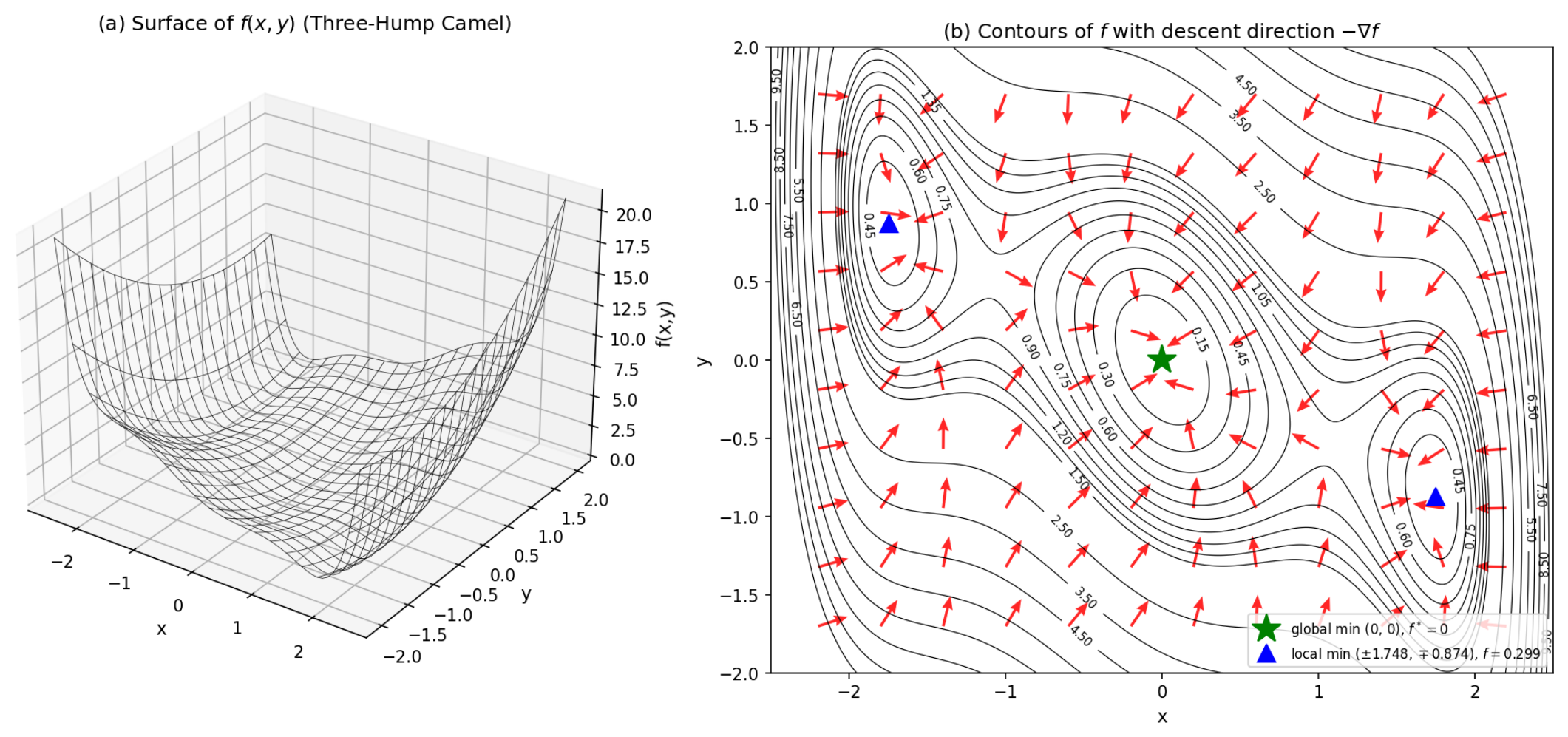
Figure 3.
First-order partial derivatives of . (a) , whose zero set is a quintic curve in y. (b) , whose zero set is the line . The thick contours mark the zero levels; they intersect at five points — the three local minima (green star = global, blue triangles = local) and two saddle points (at ).
Figure 3.
First-order partial derivatives of . (a) , whose zero set is a quintic curve in y. (b) , whose zero set is the line . The thick contours mark the zero levels; they intersect at five points — the three local minima (green star = global, blue triangles = local) and two saddle points (at ).
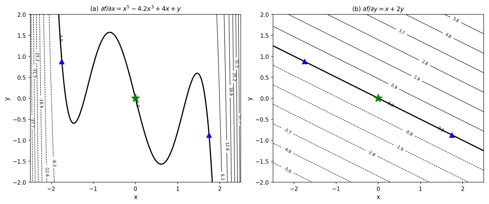
Figure 4.
The Hessian components of . (a) varies in x only; solid contours mark positive levels (convex regions), dashed contours negative (concave/saddle regions), and the thick contour the zero level. (b) is constant. (c) is constant. The three local minima are marked.
Figure 4.
The Hessian components of . (a) varies in x only; solid contours mark positive levels (convex regions), dashed contours negative (concave/saddle regions), and the thick contour the zero level. (b) is constant. (c) is constant. The three local minima are marked.
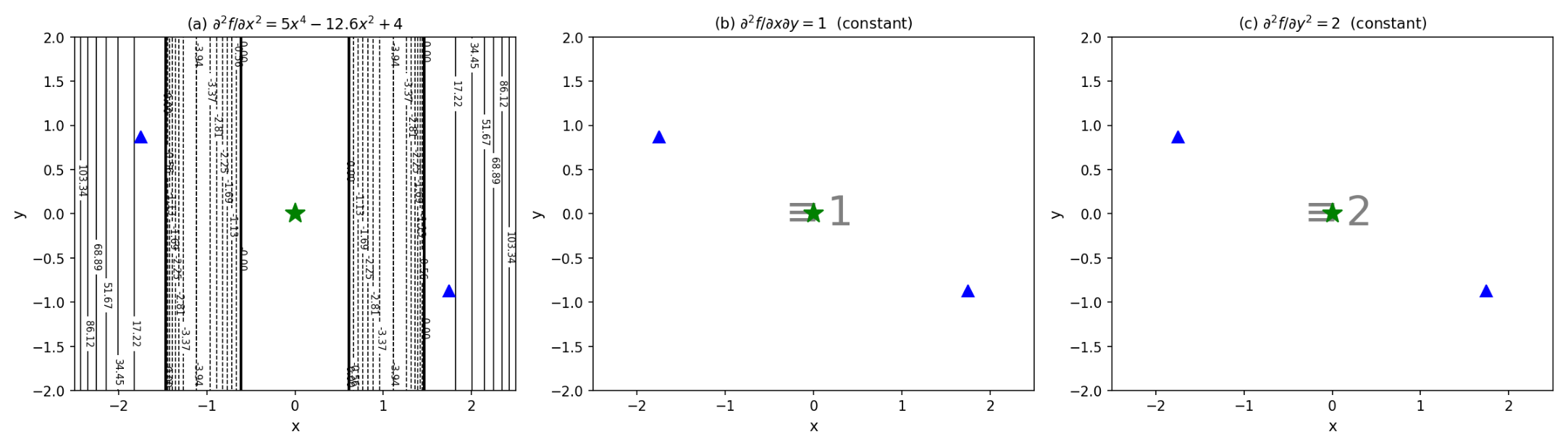
Figure 5.
Three iterative optimization methods applied to the three-hump camel function. All three start from the same point (blue triangle) and run for the same 30 iterations. The global minimum at is the black star; the two local minima at are black triangles; the position after 30 iterations is the green star. (a) Gradient descent (): ends close to the global minimum, . (b) Gauss–Newton (Levenberg–Marquardt): reaches the global minimum essentially exactly, . (c) Full Newton: trapped in the wrong basin, converging to the local minimum at with . This is a clean illustration of the central difficulty of nonlinear inversion: a more powerful local method (Newton), which uses all the second-order derivative information, can converge to a worse minimum than simple gradient descent if the local curvature pulls it into a nearby basin. The basin reached depends on the starting point, not on the sophistication of the algorithm.
Figure 5.
Three iterative optimization methods applied to the three-hump camel function. All three start from the same point (blue triangle) and run for the same 30 iterations. The global minimum at is the black star; the two local minima at are black triangles; the position after 30 iterations is the green star. (a) Gradient descent (): ends close to the global minimum, . (b) Gauss–Newton (Levenberg–Marquardt): reaches the global minimum essentially exactly, . (c) Full Newton: trapped in the wrong basin, converging to the local minimum at with . This is a clean illustration of the central difficulty of nonlinear inversion: a more powerful local method (Newton), which uses all the second-order derivative information, can converge to a worse minimum than simple gradient descent if the local curvature pulls it into a nearby basin. The basin reached depends on the starting point, not on the sophistication of the algorithm.
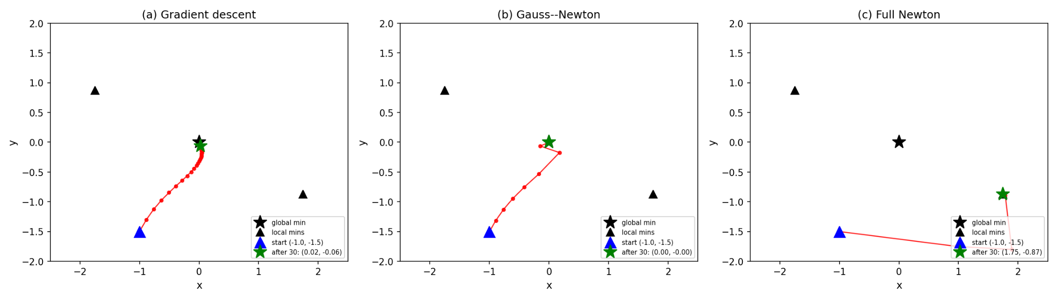
Figure 6.
Four-layer RHSF, drawn as two locomotives. The parameters are , , , and , , , , and all . Time runs from toward 0 (Remark 4), so the figure is mirror-symmetric, and two locomotives approach the endpoint from either side. They do not meet. Each one stops at its own present, . That is, stops at , at , at , and at . We draw the curve only that far, because nothing beyond it has happened yet, and the filled dots mark where each run has reached. The shaded band is empty for the same reason. It is the stretch that we have not yet travelled. It lies ahead of the present layer, and it is where we must go some day. Each panel wraps one more layer around the innermost one. That is, has the innermost layer alone, wraps one layer around it, wraps two, and wraps all four. The small gives the sharp wall in .
Figure 6.
Four-layer RHSF, drawn as two locomotives. The parameters are , , , and , , , , and all . Time runs from toward 0 (Remark 4), so the figure is mirror-symmetric, and two locomotives approach the endpoint from either side. They do not meet. Each one stops at its own present, . That is, stops at , at , at , and at . We draw the curve only that far, because nothing beyond it has happened yet, and the filled dots mark where each run has reached. The shaded band is empty for the same reason. It is the stretch that we have not yet travelled. It lies ahead of the present layer, and it is where we must go some day. Each panel wraps one more layer around the innermost one. That is, has the innermost layer alone, wraps one layer around it, wraps two, and wraps all four. The small gives the sharp wall in .
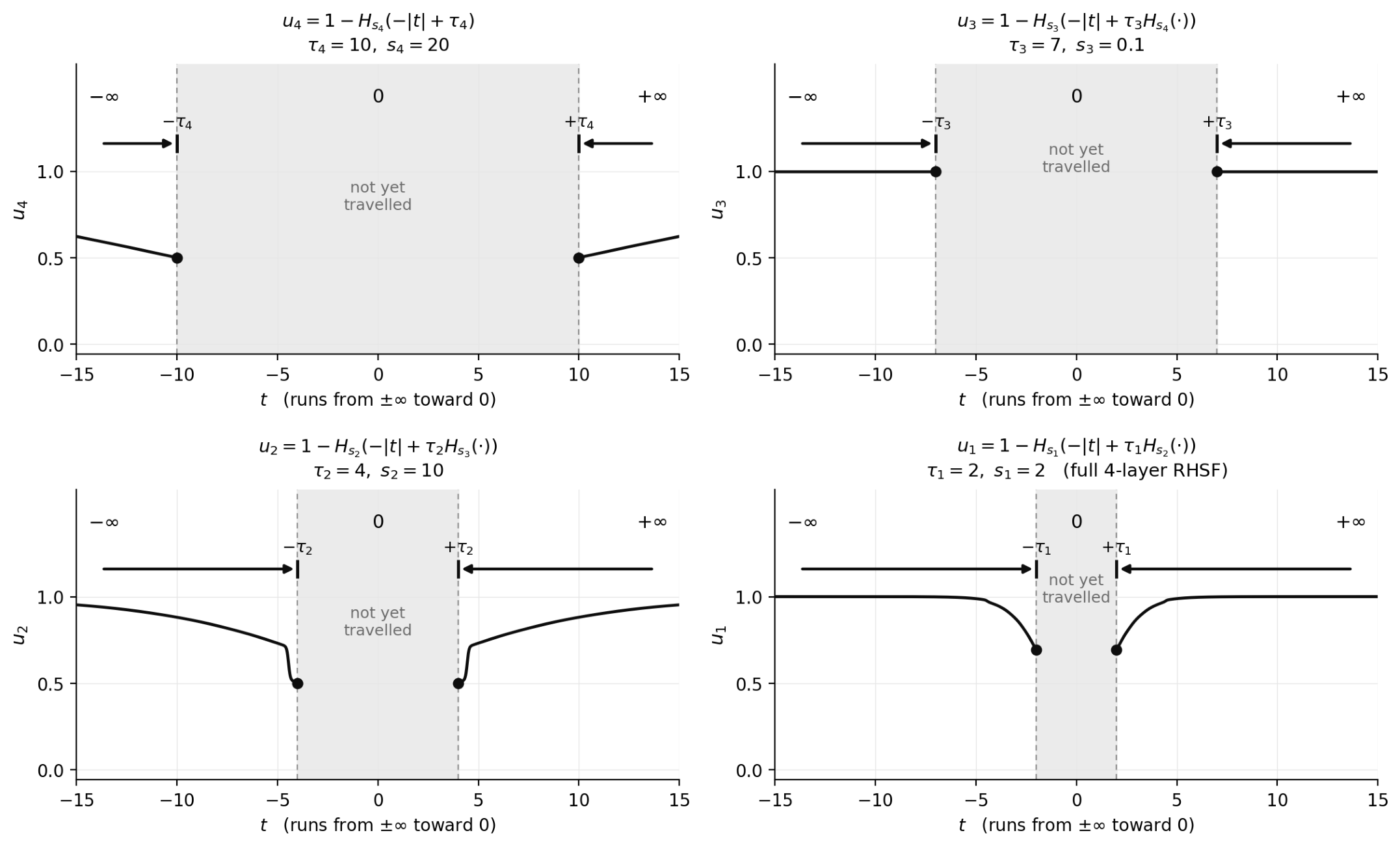
Figure 8.
The rectangle, the locomotive and the residual. Time flows from to 0, so the past lies to the right and the future lies to the left. The outer box is the rectangle , which is the whole run, filled to the end. The shaded region under the curve is the locomotive , that is, how far the run has come. What is left over is the residual , which is the blank that still lies between the present and the endpoint. The objective is . When we minimize it, we close that blank, so . Here 1 is not extinction. It is the locomotive that has arrived at its destination.
Figure 8.
The rectangle, the locomotive and the residual. Time flows from to 0, so the past lies to the right and the future lies to the left. The outer box is the rectangle , which is the whole run, filled to the end. The shaded region under the curve is the locomotive , that is, how far the run has come. What is left over is the residual , which is the blank that still lies between the present and the endpoint. The objective is . When we minimize it, we close that blank, so . Here 1 is not extinction. It is the locomotive that has arrived at its destination.
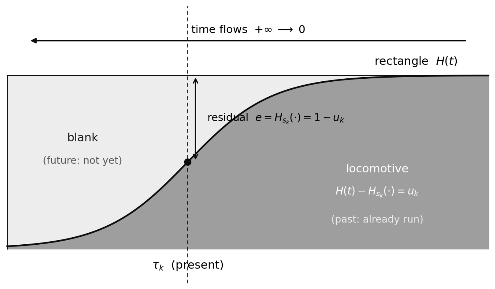
Figure 9.
One step of planning as a truncated expansion. The agent stands at one point of the parameter landscape. That point is the present , and it is the centre of expansion. The balloon contains the plan, which is a day on Bukhansan. The agent borrows the gear, climbs the path, takes a meal at the temple, looks out from the summit, and descends. None of the four scenes has occurred, and nothing outside the agent supplied any of them. The agent assembles each one from the derivatives evaluated at the point where it stands, and the cross term carries the relation between the temple meal and the summit view. The line beneath is the leading part of (56). This is local extrapolation, and it is not foresight. When the displacement exceeds the radius (64), the landscape loses its plausibility (§9).
Figure 9.
One step of planning as a truncated expansion. The agent stands at one point of the parameter landscape. That point is the present , and it is the centre of expansion. The balloon contains the plan, which is a day on Bukhansan. The agent borrows the gear, climbs the path, takes a meal at the temple, looks out from the summit, and descends. None of the four scenes has occurred, and nothing outside the agent supplied any of them. The agent assembles each one from the derivatives evaluated at the point where it stands, and the cross term carries the relation between the temple meal and the summit view. The line beneath is the leading part of (56). This is local extrapolation, and it is not foresight. When the displacement exceeds the radius (64), the landscape loses its plausibility (§9).
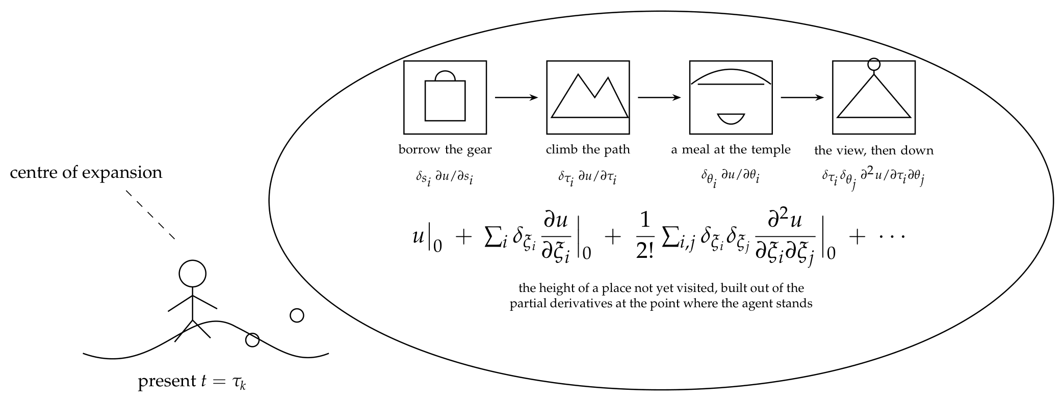
Figure 10.
Rejected coefficient vectors. Each sheet on the floor is one cognitive act in the sense of Definition 1. It is a coefficient vector c that the agent chose over the dictionary of partial derivatives at the present point, evaluated against the objective, and rejected. The dictionary was identical in every one of them. The same , the same , and the same cross terms are present at the standing point, whether or not a given combination reaches for them. What differed was c and the displacements . Some diverged because , and others remained in cliché because (§9). This is why revision is laborious. A revision is not the addition of one term. It is the re-solution of the whole coefficient problem. It is also why the sheets are not waste. By §1.17, each rejected attempt winds on as a layer and shifts the centre of expansion, so the room fills and the agent expands the next series about a different point.
Figure 10.
Rejected coefficient vectors. Each sheet on the floor is one cognitive act in the sense of Definition 1. It is a coefficient vector c that the agent chose over the dictionary of partial derivatives at the present point, evaluated against the objective, and rejected. The dictionary was identical in every one of them. The same , the same , and the same cross terms are present at the standing point, whether or not a given combination reaches for them. What differed was c and the displacements . Some diverged because , and others remained in cliché because (§9). This is why revision is laborious. A revision is not the addition of one term. It is the re-solution of the whole coefficient problem. It is also why the sheets are not waste. By §1.17, each rejected attempt winds on as a layer and shifts the centre of expansion, so the room fills and the agent expands the next series about a different point.
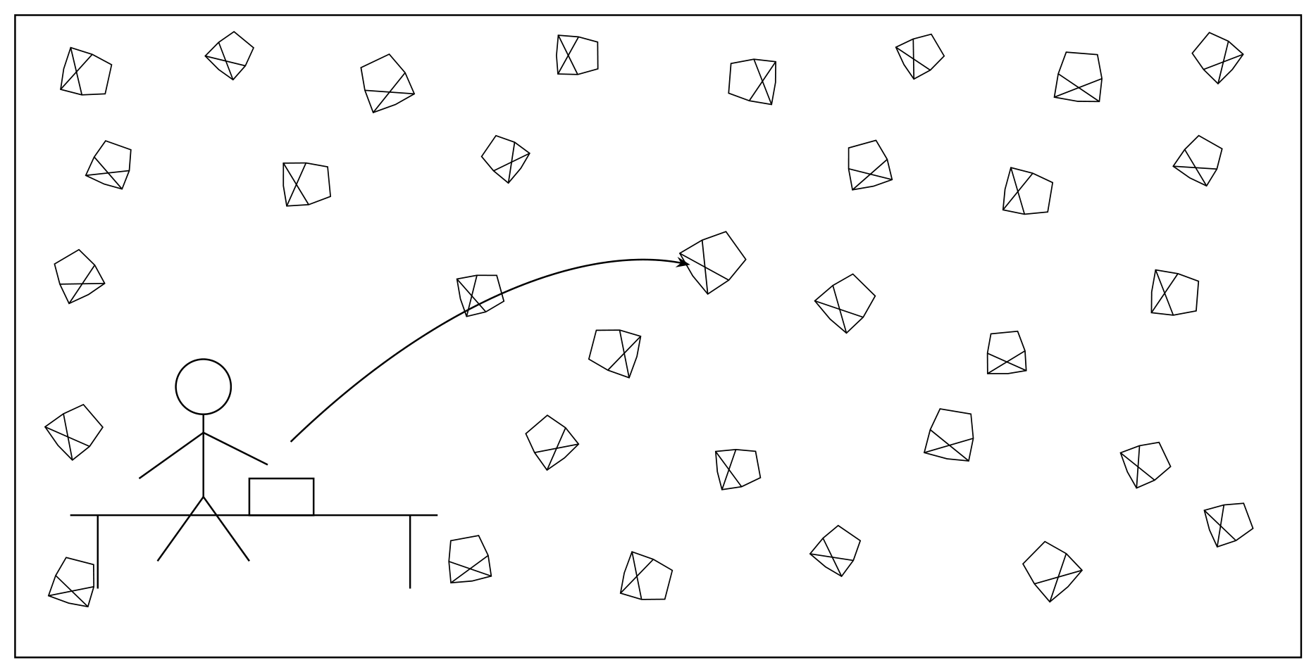
Disclaimer/Publisher’s Note: The statements, opinions and data contained in all publications are solely those of the individual author(s) and contributor(s) and not of MDPI and/or the editor(s). MDPI and/or the editor(s) disclaim responsibility for any injury to people or property resulting from any ideas, methods, instructions or products referred to in the content. |
© 2026 by the authors. Licensee MDPI, Basel, Switzerland. This article is an open access article distributed under the terms and conditions of the Creative Commons Attribution (CC BY) license (http://creativecommons.org/licenses/by/4.0/).
Copyright: This open access article is published under a Creative Commons CC BY 4.0 license, which permit the free download, distribution, and reuse, provided that the author and preprint are cited in any reuse.