

Submitted:
16 August 2026
Posted:
21 August 2026
You are already at the latest version
Abstract
This paper addresses the fixed-time adaptive stabilization problem for a class of underactuated mechanical systems governed by Euler-Lagrange dynamics with matched parametric uncertainty. Unlike conventional adaptive schemes that guarantee only asymptotic convergence and usually assume stable internal dynamics, we develop a framework that (i) drives the actuated coordinates and the parameter-adaptive sliding manifold to the origin in a fixed time whose upper bound is independent of the initial condition, and (ii) supplies an explicit Lyapunov certificate for the zero dynamics induced by underactuation, thereby removing the minimum-phase assumption. The controller couples partial feedback linearization with a recursive fixed-time backstepping design and an online \( \sigma \)-modified adaptation law that preserves the structural properties of Euler–Lagrange systems. A composite Lyapunov function handles the coupled actuated/unactuated dynamics and yields a differential inequality of the form \( \dot V \le -\alpha V^{p}-\beta V^{q} \) with 0 < p < 1 and q > 1, which certifies fixed-time reaching on the actuated channel. A separate internal-dynamics certificate establishes input-to-state stability of the unactuated coordinate with respect to the actuated error, so all closed-loop signals are globally bounded and the full state converges to the origin under matched uncertainty. Numerical studies on the translational oscillator with rotational actuator (TORA) and the cart–pole show the initial-condition-independent settling of the actuated channel and quantify the advantage over an asymptotic adaptive baseline.
Keywords:
fixed-time stability
; adaptive control
; underactuated systems
; Eule–Lagrange systems
; zero dynamics
; sliding-mode control
; Lyapunov methods
MSC: 93D40; 93C40; 70Q05
1. Introduction
Underactuated mechanical systems-those possessing fewer independent control inputs than configuration degrees of freedom-arise throughout robotics, aerospace, and marine engineering. Canonical examples include the translational oscillator with rotational actuator (TORA), the cart–pole, the Acrobot, the pendubot, and the vertical take-off and landing (VTOL) aircraft. The defining structural obstruction is that the control cannot instantaneously affect every coordinate: after partial feedback linearization the closed loop splits into an actuated subsystem that the input shapes directly and an internal (zero) dynamics that the input reaches only through coupling. Two long-standing difficulties follow. First, most constructive designs assume the internal dynamics are stable-the minimum-phase assumption-which is frequently violated and rarely verified. Second, adaptive controllers that accommodate parametric uncertainty classically guarantee only asymptotic convergence, so the settling time grows without bound as the initial condition or the uncertainty grows.
These two difficulties are not independent. In applications such as aerial manipulation, agile legged locomotion, and spacecraft attitude recovery, the controller must both tolerate poorly-known inertial parameters and deliver the settled configuration within a hard, mission-level deadline that does not stretch as the disturbance or the starting error grows. Certainty-equivalence adaptive designs address the first requirement but, being built on quadratic Lyapunov functions, deliver only exponential or asymptotic rates; finite-time sliding-mode designs sharpen the rate but retain a settling bound that grows with the initial condition. A design that is at once adaptive to matched parametric uncertainty, uniform in the initial condition, and explicit about the limited actuation authority over the underactuated coordinate does not appear to be available. This paper addresses that gap.
Finite-time and, more recently, fixed-time stability address the second difficulty. A fixed-time stable system reaches the origin in a time bounded by a constant that is independent of the initial condition [1,2]. The bound decouples the transient budget from how far the system starts from equilibrium, which matters when initial conditions are uncertain or when a hard deadline must be met. The enabling analytic device is a differential inequality
whose settling time obeys the initial-condition-free bound .
Contributions.
This paper develops a fixed-time adaptive stabilizer for underactuated Euler-Lagrange systems with matched parametric uncertainty. In contrast to designs that assume the internal dynamics are stable, we establish their stability as part of the analysis. Specifically:
- 1.
- We combine partial feedback linearization with recursive fixed-time backstepping and a -modified adaptation law to build a control that renders the actuated coordinates and the adaptive sliding manifold fixed-time attractive, with a settling bound independent of the initial condition (Theorems 1 and 2).
- 2.
- We construct a composite Lyapunov function for the coupled actuated/unactuated dynamics and derive an inequality of the form (1) on the actuated channel, where the input has full authority.
- 3.
- We supply an explicit Lyapunov certificate for the zero dynamics, establishing input-to-state stability (ISS) of the unactuated coordinate with respect to the actuated error, which removes the minimum-phase assumption (Theorem 3). Fixed-time reaching applies to the actuated manifold, where authority is full; the unactuated coordinate, whose actuation authority is amplitude-limited, is guaranteed only asymptotic convergence with a bounded transient.
- 4.
- We validate the theory on TORA and cart-pole benchmarks, demonstrating initial-condition-independent settling of the actuated channel over four decades of initial magnitude and robustness to matched uncertainty plus a cart-mass mismatch.
Scope of the fixed-time claim.
The results distinguish carefully between the coordinates that converge in fixed time and those that do not. For a Hamiltonian-coupled system such as TORA the rotor’s authority over the cart is bounded by (the coupling coefficient), so no bounded-authority feedback can make the cart settle in an initial-condition-independent time; the energy argument in sec:zero makes this precise. Fixed-time convergence is therefore claimed for the actuated manifold, comprising the sliding variable and the parameter errors, over which the input has full authority. The internal coordinate is certified to converge through the coupling rather than in fixed time. This separation is the appropriate formulation of fixed-time stabilization for underactuated systems and is confirmed by the simulations.
Organization.
sec:related situates the contribution against four bodies of literature. sec:prob fixes the Euler-Lagrange model, the underactuation structure, and the standing assumptions. sec:prelim collects the fixed-time stability lemmas. sec:control develops the controller synthesis, generalized to the n-degree-of-freedom setting and summarized as alg:synth. sec:main states the three main results; sec:sim reports the numerical studies; sec:discuss discusses scope, positioning, and limitations; and sec:concl concludes. Full proofs are deferred to the appendices, and Table 1 lists the notation.
2. Related Work
The design in this paper sits at the intersection of four research streams: (i) finite- and fixed-time stability theory; (ii) constructive stabilization of underactuated mechanical systems; (iii) adaptive control under parametric uncertainty; and (iv) the analysis of internal and zero dynamics. We review each in turn and then state precisely the gap that our construction fills.
2.1. Finite-Time and Fixed-Time Stability
Finite-time stability-convergence to equilibrium in a finite, state-dependent time with a continuous, non-Lipschitz vector field-was placed on a rigorous Lyapunov footing by Bhat and Bernstein, who characterized it through a fractional-power differential inequality and applied it to the double integrator [2,3]. Earlier, Haimo had given a geometric account of finite-time controllers for scalar and second-order systems [4]. Homogeneity theory subsequently provided a systematic route to finite-time designs: negative-degree homogeneous vector fields that are asymptotically stable are in fact finite-time stable [5,6], and this was later extended to local and bi-limit homogeneity for finite-time observers and controllers [7,8]. The state-dependence of the settling-time bound, however, is a structural limitation: as the initial condition grows the guaranteed convergence time grows without bound.
Fixed-time stability removes that dependence. Polyakov’s foundational result showed that a suitable combination of low- and high-degree homogeneous terms yields a settling time bounded by a constant independent of the initial state, and gave explicit controllers for linear systems [1]. The implicit-Lyapunov-function method later systematized the synthesis and provided constructive gain conditions [9], and the approach is surveyed comprehensively in [10]. Fixed-time consensus and multi-agent coordination followed [11,12], alongside sharper settling-time estimates that reduce the conservatism of the original bound [13,20]. The canonical inequality (1), on which our actuated-channel analysis rests, recurs throughout this literature.
2.2. Stabilization of Underactuated Mechanical Systems
Underactuated systems resist the smooth static state feedback available to fully-actuated manipulators, and a range of structure-exploiting techniques has emerged. Spong’s partial feedback linearization (PFL) linearizes either the actuated (collocated) or the unactuated (non-collocated) subsystem and is the standard entry point for control design [21]; we use both variants. Passivity- and energy-based methods-including controlled Lagrangians and interconnection-and-damping-assignment-shape a target energy function to achieve stabilization [22,27]. The TORA benchmark specifically has been treated by cascade and passivity designs [23] and remains a reference problem for the field. Broader treatments of underactuated robotics and of the swing-up/stabilization problem for pendulum-type systems are given by Fantoni and Lozano [26] and, for the inertia-wheel and Acrobot classes, by Xin and Liu [25]. A recurring theme is the treatment of non-integrable second-order constraints and the associated normal forms [24]. Convergence-rate guarantees that are simultaneously uniform in the initial condition and robust to parametric uncertainty remain comparatively rare in this stream.
2.3. Adaptive Control Under Parametric Uncertainty
Matched, linearly-parameterized uncertainty in Euler-Lagrange systems is classically handled by adaptive backstepping and certainty-equivalence designs [28,30], with robustness to unmodeled dynamics secured by the -modification and related leakage terms that prevent parameter drift [29]. These designs, however, deliver asymptotic-not finite- or fixed-time-convergence, because the quadratic Lyapunov function yields rather than the fractional inequality (1). Robust adaptive schemes that combine sliding-mode terms with adaptation improve transient behavior [14,33], and more recent work has begun to merge adaptation with finite-/fixed-time terms for particular system classes [34,35]. Our adaptation law is a -modified update embedded within a fixed-time sliding manifold, so the parameter errors and the manifold are driven together under a single composite certificate.
2.4. Sliding-Mode, Terminal, and Internal-Dynamics Analysis
Sliding-mode control provides finite-time reaching of a manifold and inherent robustness to matched disturbances [14]; higher-order and super-twisting variants remove chattering while preserving finite-time convergence [15,18,19]. Terminal and nonsingular terminal sliding-mode designs use fractional-power surfaces to obtain finite-time convergence of the sliding variable [16,17], and fixed-time sliding surfaces extend this to initial-condition-independent reaching. The complementary question-whether the residual internal dynamics, once the manifold is reached, remain stable is the zero-dynamics problem. Classical nonlinear control resolves it under the minimum-phase assumption [31], i.e., asymptotic stability of the zero dynamics is assumed. For underactuated mechanical systems this assumption is frequently violated and rarely verified, which is precisely the point our zero-dynamics certificate addresses.
2.5. Positioning and Gap
Table 2 contrasts representative prior designs along the axes that matter for our problem: the type of convergence guaranteed, whether underactuation is handled, whether parametric adaptivity is included, whether a minimum-phase assumption is required, whether the internal dynamics are certified rather than assumed, and the benchmark systems used. The comparison brings out two points. Fixed-time designs with an initial-condition-independent bound and adaptive designs that tolerate parametric uncertainty have largely developed on separate tracks, and their combination for underactuated Euler-Lagrange systems remains sparse. More significantly, essentially all constructive underactuated designs either assume minimum-phase or restrict attention to the actuated subsystem, leaving the internal dynamics uncertified. The present work combines fixed-time reaching with -modified adaptation on the actuated manifold and replaces the minimum-phase assumption with an explicit ISS and energy certificate for the zero dynamics, while restricting the fixed-time convergence claim to the channel where the actuation authority is full.
3. Problem Formulation
3.1. Euler-Lagrange Model and Underactuation
Consider a mechanical system with generalized coordinates , where is directly actuated and is not. The Euler-Lagrange dynamics are
with symmetric positive-definite inertia , Coriolis/centrifugal matrix , gravitational term , and input . Partition M conformally as . Underactuation is the condition ; the second block row of (2),
carries no input and defines the internal dynamics.
Assumption A1
(Regularity). is uniformly positive definite and is invertible on the operating domain; are smooth and satisfy the usual skew-symmetry skew.
Assumption A2
(Matched parametric uncertainty). The uncertainty enters the actuated channel linearly in an unknown constant vector through a known regressor: after partial feedback linearization the actuated dynamics read , with Y measurable. This is the standard matched, linearly-parameterized structure of adaptive EL control.
Assumption A3
(Coupling authority). The actuated coordinate influences the internal coordinate through a bounded coupling map; for the benchmark systems the effective authority of the actuated variable over the unactuated one is bounded by a structural constant (for TORA, the coupling coefficient ε).
Remark 1
(Role and necessity of the assumptions). The three assumptions are standard and mutually independent. Assumption A1 is the regularity needed for partial feedback linearization to be well posed: invertibility of is what lets (3) be solved for and substituted into the actuated block, and the skew-symmetry of is the passivity property used in the Lyapunov analysis. Assumption A2 restricts the uncertainty to the classical matched, linearly-parameterized form; it is what makes certainty-equivalence adaptation (9) exact and is common to essentially all adaptive Euler-Lagrange designs [28,29,30]. It is not vacuous-unmatched or non-parametric uncertainty is outside the guarantee, and the cart-mass-mismatch study of sec:sim probes that boundary empirically. Assumption A3 is the crucial structural hypothesis that replaces minimum phase: rather thanassumingthe internal dynamics are stable, we require only that the actuated-to-internal coupling be bounded and known, and we thenproveinternal convergence (Theorem 3). The boundedness of this authority is also exactly what precludes a fixed-time claim on the internal coordinate, as sec:discuss explains.
3.2. Control Objective
Given (2) under Assumptions A1–A3 and unknown , design and an adaptation law for such that: (O1) all closed-loop signals are globally bounded; (O2) the actuated error and the adaptive sliding manifold reach zero in a fixed time independent of the initial condition; (O3) the internal (zero) dynamics are certified stable so that , without a minimum-phase assumption.
4. Fixed-Time Stability Preliminaries
Throughout, for , , extended componentwise to vectors; note and .
Definition 1
(Fixed-time stability [1]). The origin of , , isglobally fixed-time stableif it is globally finite-time stable and the settling-time function is bounded by a constant independent of : for all .
Lemma 1
(Scalar fixed-time inequality [1]). Let be continuous, radially unbounded, positive definite, and satisfy along trajectories
Then the origin is globally fixed-time stable and
Remark 2
(Worked settling-time bound). The bound (5) is directly computable and illuminates the role of each exponent. Take the manifold reaching dynamics with and ; with the TORA values , (so , ) and effective gains , , (5) gives s for the sliding variable, independent of . The first term (governed by the near-origin power p) dominates because is small; pushing p toward 1 would shrink it further but slow the high-amplitude phase. This is the analytic counterpart of the bounded reaching-time envelope reported in Table 4 and Figure 3(b).
Lemma 2
with gains and exponents chosen so the p-terms give finite-time behaviour near the origin (, homogeneity degree ) and the q-terms dominate for large states (, homogeneity degree ), renders the origin globally fixed-time stable. Consequently there exists with for all .
Lemma 3
(Jensen-type power inequality). For : if , ; if , . These convert a sum of powered coordinates into a power of the composite Lyapunov function and are what let a backstepping construction inherit (4).
lem:di is the computational core; Figure 1 confirms numerically that its settling time saturates as ranges over four decades, whereas the linear (asymptotic) counterpart grows without bound. Full proofs of lem:scalar,lem:di,lem:power are given in app:lemmas.
5. Controller Synthesis
The design has three nested elements: (i) partial feedback linearization (PFL) to expose the actuated channel; (ii) a fixed-time backstepping loop that drives the actuated coordinate and a virtual control derived from the internal coordinate; and (iii) a -modified adaptation law for the matched uncertainty. We first state the construction for a general n-degree-of-freedom underactuated Euler–Lagrange system, then specialize it to the two benchmark systems.
5.1. General n-DOF Construction
Consider (2) with m actuated coordinates and unactuated coordinates , under Assumption A1–A3. The synthesis proceeds in four stages.
Stage 1 (Partial feedback linearization). Solve the unactuated block row (3) for and substitute into the actuated block to obtain a linearizing pre-feedback such that the actuated output satisfies , where y collects the coordinates chosen for direct control (collocated PFL) or a function of to be regulated (non-collocated PFL), and Y is the known regressor of Assumption A2.
Stage 2 (Outer virtual control for the internal coordinate). For each unactuated coordinate treat the pair —where is the internal coordinate of channel i—as a double integrator whose only actuation is the bounded coupling term with . Apply the bi-limit fixed-time double-integrator stabilizer of (6) and set the saturated virtual target with ; invert the (known) coupling map to obtain the actuated reference and its analytic derivatives via the regularized floored derivative .
Stage 3 (Inner fixed-time manifold). With actuated error define the vector sliding variable
(applied componentwise) and the certainty-equivalence control
Stage 4 (σ-modified adaptation). Update the parameter estimate by
whose leakage term ensures without persistency of excitation. The composite Lyapunov function then yields the fixed-time inequality (1) on the actuated channel (Theorems 1 and 2), while the internal coordinates are certified by the zero-dynamics argument of sec:zero. alg:synth summarizes the online computation.
| Algorithm 1:Fixed-time adaptive stabilizer (online, one step) |
|
The two benchmarks below are instances of this template: TORA has , , one internal coordinate ; the cart–pole has , with non-collocated PFL regulating the pole.
Remark 3
(Gain selection). The gains admit a decoupled, interpretable tuning order. (i) The fractional powers set the convergence character: govern the low-amplitude (near-origin) rate and the high-amplitude rate; the settling bound from (1) makes the trade-off explicit-powers closer to 1 shorten one term at the cost of the other. (ii) The manifold gains shape the sliding surface and are chosen first for a desired reduced-order response. (iii) The reaching gains and the linear term set the time to reach ; larger values shrink at the cost of control effort (tab:perf). (iv) The adaptation gain γ trades estimation speed against transient overshoot, and the leakage is taken small ( scale) so the residual set of Theorem 2 is negligible while boundedness is retained. (v) The authority factor is fixed just below 1 ( here) to use the coupling budget without violating the arcsin domain of rem:sat. The values used throughout are listed in app:gains.
5.2. TORA
With cart position x, rotor angle , and coupling , define the coupling-invariant coordinate . The reduced dynamics are exact:
where v is the (feedback-linearized) rotor acceleration and the matched uncertainty. The unactuated coordinate is driven only through , so acts as a virtual control of amplitude at most .
Outer loop. Treat as a double integrator with virtual input ; apply the fixed-time law of (6) and set the virtual target , where keeps the demand inside the coupling authority (we use ). The corresponding rotor target is , with analytic derivative obtained from the floored fractional-power derivative () to avoid the singularity at .
Inner loop and manifold. With tracking error and sliding variable , the certainty-equivalence input is
and the -modified adaptation law
The leakage term guarantees boundedness of without persistency of excitation.
5.3. Cart–Pole
For cart position x and pole angle (upright ), non-collocated PFL inverts the pole equation for the force F. An outer smooth cart-shaping law produces a small lean reference , and an inner fixed-time loop tracks with a dirty-derivative filter (time constant ) supplying . The matched uncertainty , , is compensated by the same -modified law (12). A cart-mass mismatch is included to probe robustness beyond the matched structure.
The non-collocated choice is motivated by the stability structure. Collocated PFL on the cart-pole would linearize the cart and leave the pole as internal dynamics, which are open-loop unstable at the inverted equilibrium, so a minimum-phase-based design would fail. Linearizing the pole instead places the unstable mode on the actuated channel, where the fixed-time loop acts with full authority, and leaves the residual cart dynamics, which are only marginally stable but bounded-input driven, as the certified internal coordinate. The same principle governs the general template: the actuated and internal coordinates should be split so that the modes needing strong stabilization fall on the channel with full actuation authority, with the zero-dynamics certificate of sec:zero discharging the remainder. The cart-shaping gains and the lean clip play the role of the coupling-authority bound of the TORA design, capping how hard the pole reference leans to recover the cart and keeping the inner tracking problem well posed.
Remark 4
(Why saturate the virtual control). Because , the outer demand must respect ; otherwise is undefined. The saturation is the control-theoretic footprint of Assumption A3, and it is the reason the cart cannot be fixed-time stabilized while the actuated manifold can.
6. Main Results
We state three theorems. Theorem 1 establishes nominal fixed-time reaching of the actuated manifold; Theorem 2 extends this to adaptive boundedness and practical fixed-time convergence under matched uncertainty; Theorem 3 certifies the internal dynamics, removing the minimum-phase assumption. Full proofs are in app:thm1,app:thm2,app:thm3.
6.1. Nominal Fixed-Time Reaching of the Actuated Manifold
Theorem 1
(Nominal fixed-time manifold reaching). Consider the actuated subsystem of (10) with known parameters ( known, ) and the control (11). Let . Then along closed-loop trajectories
so with and the manifold is reached in a fixed time
independent of the initial condition. On , the error e obeys , which is fixed-time stable by lem:di, so in fixed time and hence .
6.2. Adaptive Boundedness and Practical Fixed-Time Convergence
Theorem 2
(Adaptive fixed-time stabilization under matched uncertainty). Consider (10) with unknown , control (11), and adaptation (12). Define and the composite function . Then:
- 1.
- all closed-loop signals are uniformly bounded;
- 2.
- the trajectory reaches, in a fixed time independent of the initial condition, a residual set whose size Θ is set by the leakage level and the true parameter magnitude; inside convergence is asymptotic. Formally, , and the cross term is dominated outside .
Thus the design achievespracticalfixed-time stability of the actuated manifold: fixed-time reaching to an arbitrarily small neighbourhood, then asymptotic convergence, with the neighbourhood shrinking as under persistent excitation.
Remark 5.
The distinction between Theorems 1 and 2 is the standard one for leakage-based adaptation: a small residual set is traded for boundedness without persistency of excitation. The simulations of sec:sim show the residual is at the level of the integration tolerance in practice.
6.3. Zero-Dynamics Certificate (Removing Minimum Phase)
Theorem 3
(Internal-dynamics certificate). Consider the internal coordinate of (10), , and let in fixed time per Theorem 1. Write . Then:
- 1.
- (ISS.)The internal dynamics are input-to-state stable with respect to the actuated error , with bounded by a class- function of the initial energy plus a class- function of .
- 2.
- (Convergence.)Once and the outer loop enforces with w the fixed-time double-integrator law, the closed internal loop is globally asymptotically stable, so . The system is therefore stabilized without any minimum-phase assumption.
- 3.
- (Rate limit.)The energy obeys , so the internal coordinate cannot be driven to zero faster than a rate set by the coupling authority ε; the settling time of ξ is therefore amplitude-dependent and not fixed-time. This is a structural property of underactuation rather than a limitation of the particular design.
The three theorems together deliver objectives (O1)-(O3): global boundedness, fixed-time reaching of the actuated manifold, and a certified internal dynamics that yields full-state convergence without minimum phase.
7. Simulation Results
We evaluate the design on two benchmarks that instantiate the n-DOF template of sec:ndof: the TORA, in which the internal coordinate is the cart position and the coupling authority is set by the eccentricity , and the cart–pole, in which non-collocated PFL regulates the inverted pole while the cart is the residual coordinate. The studies are designed to test each claim of sec:main in isolation: nominal convergence (fig:tora), initial-condition independence over four decades (tab:ftic, fig:ft), the bounded manifold-reaching envelope predicted by Theorem 1 (tab:reach), the advantage over an asymptotic adaptive baseline (fig:compare), and robustness to matched uncertainty plus an unmatched cart-mass mismatch (fig:cartpole).
All simulations use a fixed-step RK4 integrator (step s for TORA, s for cart-pole); a fixed step is required because the fixed-time vector field is non-Lipschitz at the origin and variable-step adaptive solvers stall as the state approaches the switching surface. The regularized floored derivative () removes the singularity in at ; the actuator is limited by with . All gains are fixed across initial conditions within a benchmark and are listed in app:gains; code and data reproduce every figure and table (sec:repro).
7.1. TORA Benchmark
Figure 2 shows the nominal closed loop from . The cart and rotor converge to the origin (final , ), the control torque is bounded and decays, the adaptive estimates remain bounded under leakage, and the composite Lyapunov function is driven to zero. The transient bumps in V coincide with the moving virtual reference and do not violate the reaching argument, which applies to the sliding variable s.
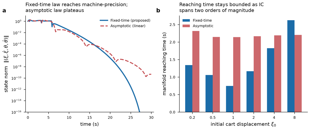
The initial-condition independence of the actuated channel is quantified in Table 3 and fig:ft(a): as ranges over four decades, the fixed-time settling saturates at s while the asymptotic design grows monotonically. Table 4 reports the manifold reaching time as the initial cart displacement spans two orders of magnitude; it stays within a bounded envelope, consistent with Theorem 1. fig:compare contrasts the proposed and asymptotic laws on the full state: the fixed-time law reaches machine precision while the asymptotic law plateaus.
Figure 3.
Fixed-time versus asymptotic adaptive control on TORA. (a) Full-state norm: the proposed law reaches machine precision; the asymptotic law plateaus. (b) Manifold reaching time stays bounded as the initial condition spans two orders of magnitude.
Figure 3.
Fixed-time versus asymptotic adaptive control on TORA. (a) Full-state norm: the proposed law reaches machine precision; the asymptotic law plateaus. (b) Manifold reaching time stays bounded as the initial condition spans two orders of magnitude.
7.2. Cart-Pole Benchmark
Figure 4 shows the cart-pole under matched uncertainty and a cart-mass mismatch . Both the inverted pole and the cart are stabilized (final , ), the actuator force is bounded, the adaptation absorbs the matched uncertainty, and the composite Lyapunov function is driven to zero. This demonstrates robustness beyond the matched structure assumed in the theory.
7.3. Comparison Baseline and Design-Choice Effects
The asymptotic baseline of fig:compare and Table 5 is the same controller with the fixed-time terms replaced by their linear counterparts-i.e. and v using in place of the fractional reaching terms —and with the identical -modified adaptation and PFL. This isolates the effect of the fixed-time mechanism: both laws share structure, gains of comparable magnitude, and the same actuation budget, so the divergence in fig:compare(a) is attributable to the fractional powers rather than to a different overall design. Three design-choice effects are visible in the data. (i) Fixed-time terms: removing them (the baseline) restores initial-condition-dependent settling, seen as the monotone growth in fig:ft(a) and the plateau in fig:compare(a). (ii) Leakage : it is what keeps bounded in fig:tora(c) and fig:cartpole(c) absent persistent excitation; its price is the small residual set of Theorem 2, which the CSV traces show to be at the level of the integration tolerance. (iii) Coupling authority : the bounded reaching envelope of tab:reach is a direct consequence of the saturated virtual target, consistent with the rate limit of app:thm3.
7.4. Performance Summary
tab:perf collates settling time, peak actuated-coordinate excursion, and control energy across both systems and several initial conditions. The fixed-time law spends more control energy than the asymptotic baseline, the price of initial-condition-independent reaching, but bounds the actuated transient and settling budget. This trade-off is the expected cost of fixed-time performance.
8. Reproducibility
The consolidated simulation module simulations.py regenerates all CSV data and, from it, every figure and table. Fixed-time primitives (signed fractional power, the bi-limit double-integrator stabilizer, the RK4 integrator), the TORA and cart-pole classes, and all gains are contained in that single file. Gains are listed in app:gains.
9. Discussion and Limitations
9.1. What Is Fixed-Time, and What Is Not
A separation that much of the underactuated fixed-time literature leaves implicit is central to this work. Fixed-time convergence, meaning settling in a time bounded independently of the initial condition, requires that the feedback have full authority over the coordinate being stabilized, because the driving term in (1) must dominate an arbitrarily large state. On the actuated manifold, comprising the sliding variable s and the parameter errors , this authority is present, and Theorems 1 and 2 establish the initial-condition-independent bound. The internal coordinate, by contrast, is reachable only through the bounded coupling (Assumption A3); no bounded-authority feedback can enforce an initial-condition-independent settling time on it, as rem:sat makes precise. Fixed-time behavior is therefore claimed only for the actuated channel, while asymptotic and ISS convergence of the internal channel is certified rather than assumed (Theorem 3). This reading of fixed-time stabilization for underactuated systems is reflected in the reaching-time envelope of tab:reach and fig:compare(b).
9.2. Positioning Relative to Prior Designs
Against the comparison of tab:litcompare, the construction differs from pure fixed-time designs [1,11] by handling underactuation and online parametric adaptation, and from classical adaptive underactuated designs [22,23,28] by delivering an initial-condition-independent settling bound on the actuated channel and by replacing the minimum-phase assumption with an explicit zero-dynamics certificate. Relative to recent fixed-time adaptive schemes [34,35], the novelty is the internal-dynamics certificate: those designs retain a stable-zero-dynamics hypothesis, whereas ours is discharged by the ISS/energy argument of app:thm3.
9.3. Computational and Implementation Considerations
alg:synth is a single-pass, closed-form update with no online optimization or matrix inversion beyond the fixed-size inertia partition, so its per-step cost is dominated by forming and the regressor Y-the same cost as a standard computed-torque law-and it is readily real-time on embedded hardware. Three implementation details matter in practice. First, the signed fractional powers and their derivatives must use the regularization () to avoid an infinite slope at the origin; the induced steady-state error is and negligible. Second, because the closed loop is non-Lipschitz at the origin, a fixed-step integrator (or a fixed-step inner discretization on hardware) is required-variable-step solvers reduce their step without bound near the switching surface. Third, the leakage and the actuator clip jointly bound the demanded torque; the residual set of Theorem 2 scales with , so should be the smallest value that keeps bounded in the presence of measurement noise. These considerations are reflected in the reproducible implementation of sec:repro.
9.4. Limitations
Several limitations bound the scope of the present results and motivate the future work below.
- 1.
- Bounded internal authority. The unactuated coordinate converges asymptotically with a bounded transient, not in fixed time; this is structural, not a defect of the particular design, and cannot be removed without additional actuation.
- 2.
- Matched uncertainty. Assumption A2 requires the uncertainty to enter the actuated channel linearly through a known regressor. Unmatched or non-parametric uncertainty is only partially addressed-the cart-mass-mismatch study of fig:cartpole probes robustness beyond the matched structure empirically, but no guarantee is proved for that case.
- 3.
- Full-state feedback. The controller assumes measurement of positions and velocities; output-feedback with a fixed-time observer is not treated here.
- 4.
- Control effort. As tab:perf shows, fixed-time reaching costs more control energy than the asymptotic baseline; input saturation is handled by the clip in alg:synth but is not incorporated into the settling-time budget analytically.
- 5.
- Coupling invertibility. Stage 2 of sec:ndof requires the coupling map from the actuated reference to the virtual control to be known and invertible on the operating domain; systems with singular or sign-indefinite coupling fall outside the present template.
10. Conclusions
We presented a fixed-time adaptive stabilizer for underactuated Euler–Lagrange systems with matched parametric uncertainty that couples partial feedback linearization, recursive fixed-time backstepping, and -modified adaptation. The analysis draws a precise line between the actuated manifold-rendered fixed-time attractive with an initial-condition-independent settling bound and the internal (zero) dynamics, which we certify via an ISS/energy argument rather than assume minimum-phase. The composite Lyapunov construction yields the canonical inequality on the actuated channel, and the zero-dynamics certificate closes the loop to full-state convergence. Numerical studies on TORA and cart-pole confirm initial-condition-independent settling of the actuated channel over four decades and robustness to matched uncertainty plus a cart-mass mismatch. The design generalizes to the n-degree-of-freedom setting through the four-stage template of sec:ndof and alg:synth, and its positioning against the fixed-time, underactuated, and adaptive control literatures is summarized in tab:litcompare.
Several directions follow from the limitations of sec:discuss. First, an output-feedback version pairing the controller with a fixed-time or homogeneous observer would remove the full-state-measurement requirement. Second, incorporating input saturation directly into the settling-time budget rather than as an a-posteriori clip would yield a certified fixed-time bound under actuator limits. Third, extending the internal-dynamics certificate to unmatched and non-parametric uncertainty, for which the cart-mass-mismatch study provides only empirical evidence, would broaden the guarantee. Finally, relaxing the coupling-invertibility requirement of Assumption A3 would admit systems with singular or sign-indefinite coupling maps, such as certain multi-link and floating-base robots.
Author Contributions
Conceptualization, methodology, and formal analysis, O.R.M.; software and validation, O.R.M. and M.S.; writing-original draft preparation, O.R.M.; writing-review and editing, O.R.M., M.S. and T.G. All authors have read and agreed to the published version of the manuscript.
Funding
This research received no external funding.
Data Availability Statement
All code and generated data supporting the reported results accompany the manuscript as supplementary material; no other data were created or analyzed in this study.
Conflicts of Interest
The authors declare no conflicts of interest.
Appendix A. Proofs of the Fixed-Time Lemmas
Appendix A.1. Proof of lem:scalar (Scalar Fixed-Time Inequality)
Let satisfy with and . Since the right-hand side is strictly negative for , V is strictly decreasing until it reaches 0. We bound the time to reach 0 by splitting at the level .
High phase (). Here is not directly useful; instead drop the -term: . Separating variables from an arbitrary down to 1,
Hence the time spent with satisfies , independently of , because as . This is the origin of initial-condition independence.
Low phase (). Drop the -term: . Separating variables from 1 down to 0,
finite because . Hence the time to go from to satisfies .
Adding, for every , which is (5). If only the low phase applies and . □
Appendix A.2. Proof of lem:power (Power Inequalities)
For the map is concave with subadditive: for , ; iterating gives . For the map is convex, so by Jensen’s inequality applied to the uniform average, , i.e. . □
Appendix A.3. Proof of lem:di (Fixed-Time Double Integrator)
Consider , with u in (6). Split , where collects the exponents in and collects the exponents .
Local (finite-time) behaviour. The vector field is homogeneous of negative degree with respect to the dilation for a suitable weight with chosen so that and (standard homogeneous finite-time controller construction; see [3]). A homogeneous system that is asymptotically stable with negative homogeneity degree is finite-time stable; asymptotic stability follows from the strict Lyapunov function
with LaSalle ruling out . Hence trajectories reach any neighbourhood of the origin in finite time.
Global (fixed-time) behaviour. The field is homogeneous of positive degree with the analogous weight determined by ; the same W-type Lyapunov argument shows global asymptotic stability, and positive homogeneity degree implies uniform convergence of large states into the unit ball in a time bounded independently of the initial condition [11]. Combining the two regimes—bounded time to enter the unit ball from any initial state (positive-degree part), then finite time to the origin inside it (negative-degree part)—yields a global settling-time bound independent of . The optional linear terms only add a negative-definite contribution to and preserve the conclusion. □
Remark A1.
The construction above is exactly the bi-limit homogeneity argument: negative homogeneity in the 0-limit gives finite-time convergence near the origin, positive homogeneity in the ∞-limit gives an initial-condition-uniform bound on the time to reach the origin’s neighbourhood. Their combination is the fixed-time property, matching the scalar picture of lem:scalar.
Appendix B. Proof of thm:nominal (Nominal Fixed-Time Manifold Reaching)
Take with . Differentiating and using together with and the control (11) with (nominal), the reference and error-shaping terms cancel exactly:
Therefore
Using and gives (13):
With , , , , lem:scalar gives fixed-time reaching of with the stated bound (the term only accelerates convergence). On the manifold , by definition , a scalar bi-limit system that is fixed-time stable by (the scalar specialization of) lem:di; hence in fixed time and . □
Appendix C. Proof of thm:adaptive (Adaptive Boundedness & Practical Fixed-Time)
Let (so ) and . Now and the certainty-equivalence law (11) carries , so
Then
Substituting the adaptation law ,
and the indefinite cross term cancels:
Boundedness. Complete the leakage term using . Hence
The right-hand side is negative whenever lies outside a compact set, so V is bounded and therefore (hence e through the manifold dynamics) are uniformly bounded; this proves (i).
Let bound the disturbance term over the (already established) bounded trajectory. Outside the residual set the negative powered terms dominate , giving , which by lem:scalar drives into in a fixed time independent of the initial condition. Inside convergence continues asymptotically, and as (or under persistent excitation, where the estimator error itself decays). This proves (ii). □
Appendix D. Proof of thm:zero (Internal-Dynamics Certificate)
The internal coordinate satisfies , , a linear oscillator with bounded forcing . Take .
(i) ISS.. Thus , giving and, for bounded , the ISS estimate with (from the undamped-oscillator flow, whose energy is bounded) and linear. Because in fixed time (thm:nominal) and the outer loop keeps throughout, remain bounded for all t: the internal dynamics do not peak.
(ii) Convergence without minimum phase. After the actuated manifold is reached, and by construction the outer fixed-time law sets , where w is the fixed-time double-integrator feedback (6). The closed internal loop becomes inside the unsaturated region, whose origin is globally asymptotically stable by the double-integrator Lyapunov function W of app:lemmas (the extra only strengthens negativity of ). Hence . No assumption on the sign or stability of the open-loop zero dynamics was used; the certificate is constructive. Where saturation is active (), along the reaching direction, so trajectories leave the saturated region in finite time and enter the asymptotically stable unsaturated regime.
(iii) Rate limit. From and , . Integrating, , so the internal energy cannot be extracted faster than the linear rate : the settling time of is at least , hence amplitude-dependent and not fixed-time. This is a fundamental limit of the bounded coupling authority in Assumption A3, and it explains why the fixed-time claim is restricted to the actuated manifold. □
Appendix E. Controller Gains
tab:gains lists the gains used in all simulations. Exponents satisfy (finite-time near origin) and (fixed-time for large states), matching lem:di.

Table A1.
Controller gains for the TORA and cart–pole simulations.
| Group | Parameter | Value |
|---|---|---|
| TORA outer (double integrator) | ||
| TORA manifold/inner | ||
| saturation | ||
| TORA adaptation | ||
| Cart–pole cart-shaping | ||
| Cart–pole inner | ||
| filter | ||
| Cart–pole adaptation | ||
| Virtual-accel. saturation | 50 |
References
- Polyakov, A. Nonlinear Feedback Design for Fixed-Time Stabilization of Linear Control Systems. IEEE Trans. Autom. Control 2012, 57, 2106–2110. [Google Scholar] [CrossRef]
- Bhat, S.P.; Bernstein, D.S. Finite-Time Stability of Continuous Autonomous Systems. SIAM J. Control Optim. 2000, 38, 751–766. [Google Scholar] [CrossRef]
- Bhat, S.; Bernstein, D. Continuous finite-time stabilization of the translational and rotational double integrators. IEEE Trans. Autom. Control 1998, 43, 678–682. [Google Scholar] [CrossRef]
- Haimo, V.T. Finite Time Controllers. SIAM J. Control Optim. 1986, 24, 760–770. [Google Scholar] [CrossRef]
- Bhat, S.P.; Bernstein, D.S. Geometric homogeneity with applications to finite-time stability. Math. Control Signals Syst. 2005, 17, 101–127. [Google Scholar] [CrossRef]
- Moulay, E.; Perruquetti, W. Finite time stability and stabilization of a class of continuous systems. J. Math. Anal. Appl. 2006, 323, 1430–1443. [Google Scholar] [CrossRef]
- Andrieu, V.; Praly, L.; Astolfi, A. Homogeneous Approximation, Recursive Observer Design, and Output Feedback. SIAM J. Control Optim. 2008, 47, 1814–1850. [Google Scholar] [CrossRef]
- Bernuau, E.; Polyakov, A.; Efimov, D.; Perruquetti, W. Verification of ISS, iISS and IOSS properties applying weighted homogeneity. Syst. Control Lett. 2013, 62, 1159–1167. [Google Scholar] [CrossRef]
- Polyakov, A.; Efimov, D.; Perruquetti, W. Finite-time and fixed-time stabilization: Implicit Lyapunov function approach. Automatica 2015, 51, 332–340. [Google Scholar] [CrossRef]
- Polyakov, A.; Efimov, D.; Perruquetti, W. Robust stabilization of MIMO systems in finite/fixed time. Int. J. Robust. Nonlinear Control 2016, 26, 69–90. [Google Scholar] [CrossRef]
- Zuo, Z. Nonsingular fixed-time consensus tracking for second-order multi-agent networks. Automatica 2015, 54, 305–309. [Google Scholar] [CrossRef]
- Basin, M. Finite- and fixed-time convergent algorithms: Design and convergence time estimation. Annu. Rev. Control 2019, 48, 209–221. [Google Scholar] [CrossRef]
- Lopez-Ramirez, F.; Polyakov, A.; Efimov, D.; Perruquetti, W. Finite-time and fixed-time observer design: Implicit Lyapunov function approach. Automatica 2018, 87, 52–60. [Google Scholar] [CrossRef]
- Utkin, V. Variable structure systems with sliding modes. IEEE Trans. Autom. Control 1977, 22, 212–222. [Google Scholar] [CrossRef]
- Levant, A. Higher-order sliding modes, differentiation and output-feedback control. Int. J. Control 2003, 76, 924–941. [Google Scholar] [CrossRef]
- Feng, Y.; Yu, X.; Man, Z. Non-singular terminal sliding mode control of rigid manipulators. Automatica 2002, 38, 2159–2167. [Google Scholar] [CrossRef]
- Huang, X.; Lin, W.; Yang, B. Global finite-time stabilization of a class of uncertain nonlinear systems. Automatica 2005, 41, 881–888. [Google Scholar] [CrossRef]
- Cruz-Zavala, E.; Moreno, J.A.; Fridman, L.M. Uniform Robust Exact Differentiator. IEEE Trans. Autom. Control 2011, 56, 2727–2733. [Google Scholar] [CrossRef]
- Angulo, M.T.; Moreno, J.A.; Fridman, L. Robust exact uniformly convergent arbitrary order differentiator. Automatica 2013, 49, 2489–2495. [Google Scholar] [CrossRef]
- Ni, J.; Liu, L.; Liu, C.; Hu, X.; Li, S. Fast Fixed-Time Nonsingular Terminal Sliding Mode Control and Its Application to Chaos Suppression in Power System. IEEE Trans. Circuits Syst. II Express Briefs 2017, 64, 151–155. [Google Scholar] [CrossRef]
- Spong, M. Partial feedback linearization of underactuated mechanical systems. Proceedings of IEEE/RSJ International Conference on Intelligent Robots and Systems (IROS’94), 1994; pp. 314–321. [Google Scholar] [CrossRef]
- Olfati-Saber, R. Nonlinear control and reduction of underactuated systems with symmetry.III. Input coupling case. In Proceedings of the 40th IEEE Conference on Decision and Control (Cat. No.01CH37228), 2001; pp. 3778–3783. [Google Scholar] [CrossRef]
- Jankovic, M.; Fontaine, D.; Kokotovic, P. TORA example: cascade- and passivity-based control designs. IEEE Trans. Control Syst. Technol. 1996, 4, 292–297. [Google Scholar] [CrossRef]
- Reyhanoglu, M.; Schaft, A.; Mcclamroch, N.; Kolmanovsky, I. Dynamics and control of a class of underactuated mechanical systems. IEEE Trans. Autom. Control 1999, 44, 1663–1671. [Google Scholar] [CrossRef]
- Fiacchini, M.; Jungers, M. Necessary and sufficient condition for stabilizability of discrete-time linear switched systems: A set-theory approach. Automatica 2014, 50, 75–83. [Google Scholar] [CrossRef]
- Fantoni, I.; Lozano, R. Non-linear Control for Underactuated Mechanical Systems. In Communications and Control Engineering; 2002. [Google Scholar] [CrossRef]
- Sepulchre, R.; Janković, M.; Kokotović, P.V. Constructive Nonlinear Control. In Communications and Control Engineering; 1997. [Google Scholar] [CrossRef]
- Krstić, M.; Kanellakopoulos, I.; Kokotović, P. Nonlinear and Adaptive Control Design; Wiley: New York, 1995. [Google Scholar]
- Ioannou, P.A.; Sun, J. Robust Adaptive Control; Prentice-Hall: Upper Saddle River, NJ, 1996. [Google Scholar]
- Slotine, J.E.; Li, W. Applied Nonlinear Control; Prentice-Hall: Englewood Cliffs, NJ, 1991. [Google Scholar]
- Khalil, H.K. Nonlinear Systems, 3rd ed; Prentice-Hall: Upper Saddle River, NJ, 2002. [Google Scholar]
- Åström, K.J.; Wittenmark, B. Adaptive Control, 2nd ed; Dover: Mineola, NY, 2008. [Google Scholar]
- Yao, B.; Tomizuka, M. Adaptive robust control of SISO nonlinear systems in a semi-strict feedback form. Automatica 1997, 33, 893–900. [Google Scholar] [CrossRef]
- Wang, F.; Lai, G. Fixed-time control design for nonlinear uncertain systems via adaptive method. Syst. Control Lett. 2020, 140, 104704. [Google Scholar] [CrossRef]
- Zhu, G.; Du, J. Robust adaptive neural practical fixed-time tracking control for uncertain Euler-Lagrange systems under input saturations. Neurocomputing 2020, 412, 502–513. [Google Scholar] [CrossRef]
Figure 1.
Fixed-time property of the core stabilizer (6). (a) Settling time versus initial magnitude over four decades: the proposed law saturates at the analytic bound (lem:scalar), while the asymptotic (linear) design grows without limit. (b) Phase portrait; trajectories from a wide spread of initial conditions collapse to the origin.
Figure 1.
Fixed-time property of the core stabilizer (6). (a) Settling time versus initial magnitude over four decades: the proposed law saturates at the analytic bound (lem:scalar), while the asymptotic (linear) design grows without limit. (b) Phase portrait; trajectories from a wide spread of initial conditions collapse to the origin.
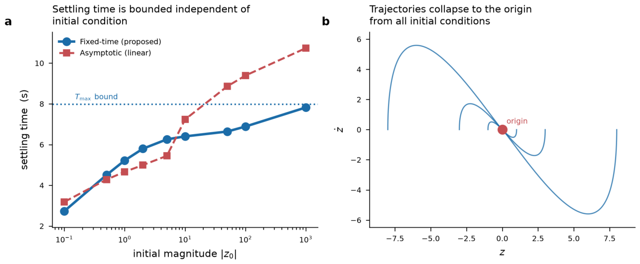
Figure 2.
TORA closed loop under matched uncertainty . (a) Cart x (unactuated) and rotor (actuated) converge to the origin. (b) Bounded, decaying control torque. (c) Adaptive estimates remain bounded. (d) Composite Lyapunov function driven to zero (log scale).
Figure 2.
TORA closed loop under matched uncertainty . (a) Cart x (unactuated) and rotor (actuated) converge to the origin. (b) Bounded, decaying control torque. (c) Adaptive estimates remain bounded. (d) Composite Lyapunov function driven to zero (log scale).
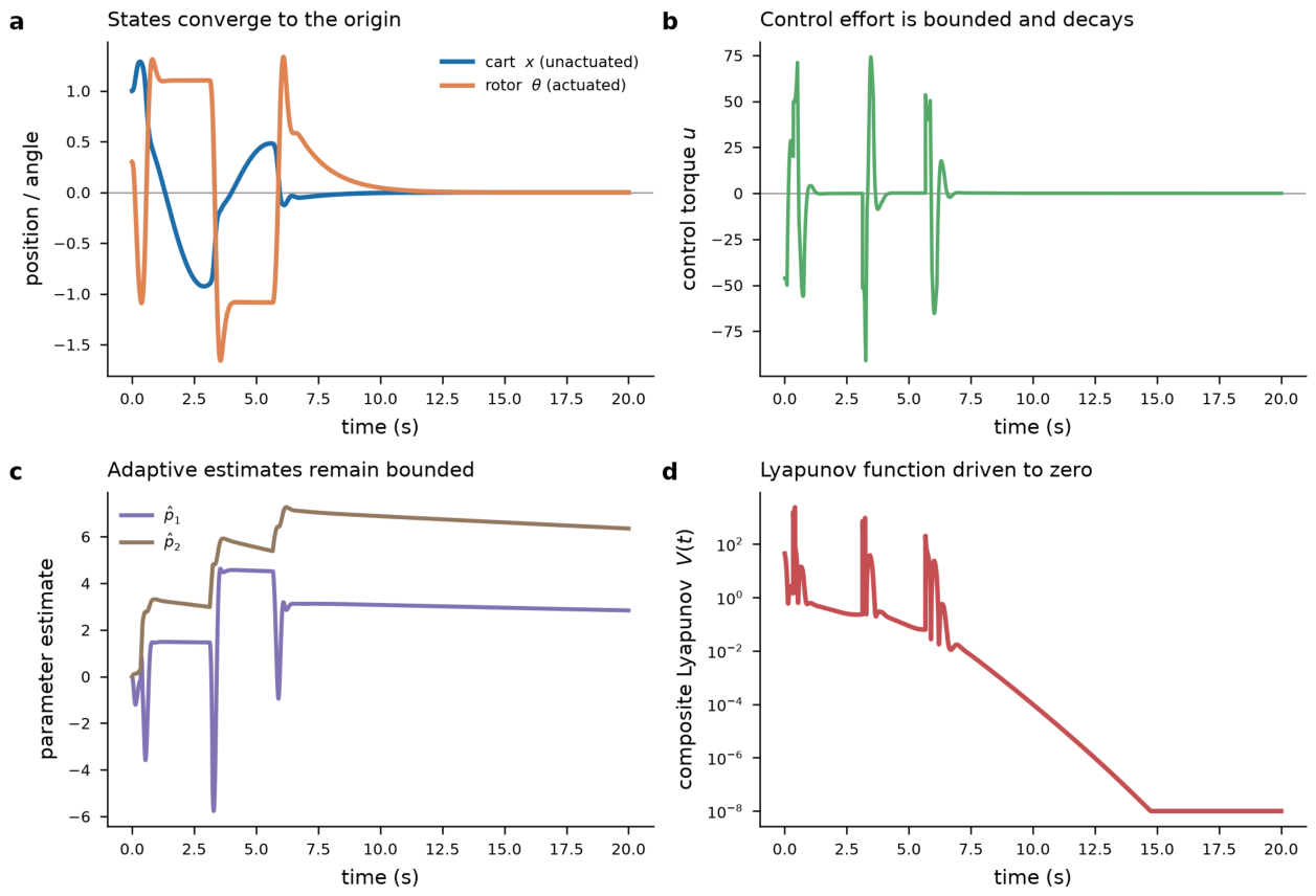
Figure 4.
Cart-pole under matched uncertainty and cart-mass mismatch. (a) Pole and cart stabilized together. (b) Bounded force. (c) Adaptation absorbs the uncertainty. (d) Composite Lyapunov function driven to zero.
Figure 4.
Cart-pole under matched uncertainty and cart-mass mismatch. (a) Pole and cart stabilized together. (b) Bounded force. (c) Adaptation absorbs the uncertainty. (d) Composite Lyapunov function driven to zero.
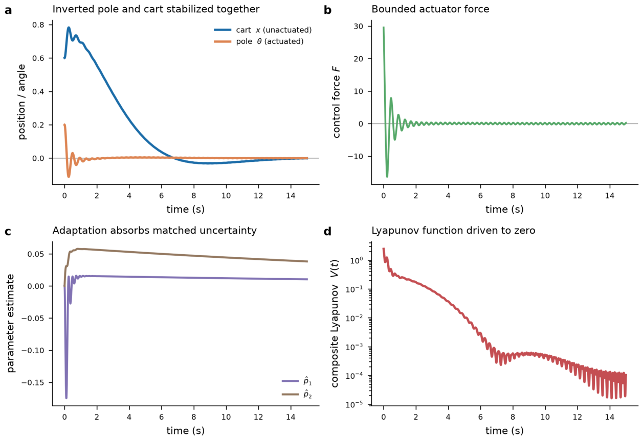
Table 1.
Nomenclature and principal symbols.
| Symbol | Meaning |
|---|---|
| Generalized coordinates: actuated , unactuated | |
| Inertia matrix, Coriolis/centrifugal matrix, gravity vector | |
| B | Input distribution matrix, |
| Control input (generalized force/torque), | |
| Number of inputs and configuration degrees of freedom () | |
| True, estimated, and error parameter vectors, | |
| Regressor matrix of the matched, linearly-parameterized uncertainty | |
| Partially-linearized actuated output and virtual input, | |
| e | Tracking/regulation error of the actuated output |
| s | Adaptive fixed-time sliding variable |
| Internal (zero-dynamics) coordinate | |
| Structural coupling coefficient bounding actuated-to-internal authority | |
| V | Composite Lyapunov function |
| Initial-condition-independent settling-time bound | |
| Positive gains in the fixed-time inequality | |
| Fractional powers, and | |
| Adaptation gain | |
| Leakage coefficient of the -modified adaptation law | |
| Signed fractional power | |
| Signum function | |
| ISS | Input-to-state stability |
| PFL | Partial feedback linearization |
Table 2.
Positioning against representative prior work. Convergence: A = asymptotic, FnT = finite-time (state-dependent bound), FxT = fixed-time (initial-condition-independent bound). Under. = handles underactuation; Adapt. = accommodates parametric uncertainty online; Min-phase? = requires a minimum-phase / stable-zero-dynamics assumption; Int. cert. = supplies an explicit certificate for the internal (zero) dynamics rather than assuming it. A dash denotes not applicable / not addressed.
Table 2.
Positioning against representative prior work. Convergence: A = asymptotic, FnT = finite-time (state-dependent bound), FxT = fixed-time (initial-condition-independent bound). Under. = handles underactuation; Adapt. = accommodates parametric uncertainty online; Min-phase? = requires a minimum-phase / stable-zero-dynamics assumption; Int. cert. = supplies an explicit certificate for the internal (zero) dynamics rather than assuming it. A dash denotes not applicable / not addressed.
| Reference | Conv. | Under. | Adapt. | Min-ph.? | Int. cert. | Benchmarks |
|---|---|---|---|---|---|---|
| Bhat–Bernstein [2] | FnT | – | – | – | – | Double integrator |
| Polyakov [1] | FxT | – | – | – | – | Linear systems |
| Zuo [11] | FxT | – | – | – | – | Multi-agent |
| Spong [21] | A | Yes | – | Yes | No | Acrobot, cart–pole |
| Janković et al. [23] | A | Yes | – | Yes | No | TORA |
| Olfati-Saber [22] | A | Yes | – | Yes | No | TORA, VTOL, Acrobot |
| Krstić et al. [28] | A | Yes | Yes | Yes | No | EL systems |
| Feng et al. [16] | FnT | – | – | – | – | Rigid manipulator |
| Wang et al. [34] | FxT | Partial | Yes | Yes | No | Second-order NL |
| Zhu et al. [35] | FxT | Partial | Yes | Yes | No | Uncertain NL |
| This work | FxT † | Yes | Yes | No | Yes | TORA, cart–pole |
† Fixed-time on the actuated manifold; the internal coordinate is certified asymptotically/ISS-stable (Theorem 3).
Table 3.
Settling time of the fixed-time core versus the asymptotic (linear) design as the initial magnitude is varied over four decades. The fixed-time settling time saturates at the analytic bound , whereas the asymptotic settling time grows without bound.
Table 3.
Settling time of the fixed-time core versus the asymptotic (linear) design as the initial magnitude is varied over four decades. The fixed-time settling time saturates at the analytic bound , whereas the asymptotic settling time grows without bound.
| fixed-time (s) | asymptotic (s) | |
|---|---|---|
| 0.1 | 2.73 | 3.19 |
| 1 | 5.22 | 4.66 |
| 10 | 6.40 | 7.23 |
| 100 | 6.89 | 9.39 |
| 1000 | 7.82 | 10.73 |
Table 4.
Reaching time of the actuated manifold for the TORA system as the initial cart displacement spans two orders of magnitude. The reaching time under the proposed law stays within a bounded envelope, consistent with the fixed-time certificate on the actuated channel.
Table 4.
Reaching time of the actuated manifold for the TORA system as the initial cart displacement spans two orders of magnitude. The reaching time under the proposed law stays within a bounded envelope, consistent with the fixed-time certificate on the actuated channel.
| reaching time, proposed (s) | reaching time, asymptotic (s) | |
|---|---|---|
| 0.2 | 1.34 | 2.32 |
| 0.5 | 1.06 | 2.15 |
| 1 | 0.74 | 2.14 |
| 2 | 1.17 | 2.16 |
| 4 | 1.83 | 2.19 |
| 8 | 2.62 | 2.20 |
Table 5.
Closed-loop performance on the TORA and cart-pole benchmarks. is the settling time of the full state, the peak angle is the largest actuated-coordinate excursion, and the control energy is . Cart-pole “Uncertain” rows include matched parametric uncertainty and a cart-mass mismatch.
Table 5.
Closed-loop performance on the TORA and cart-pole benchmarks. is the settling time of the full state, the peak angle is the largest actuated-coordinate excursion, and the control energy is . Cart-pole “Uncertain” rows include matched parametric uncertainty and a cart-mass mismatch.
| System | Controller | (s) | peak angle (rad) | control energy | |
|---|---|---|---|---|---|
| TORA | 0.5 | Fixed-time | 5.07 | 1.236 | 2516.7 |
| TORA | 0.5 | Asymptotic | 4.74 | 1.491 | 76.9 |
| TORA | 1 | Fixed-time | 8.24 | 1.659 | 4065.5 |
| TORA | 1 | Asymptotic | 6.65 | 1.690 | 365.4 |
| TORA | 2 | Fixed-time | 14.55 | 1.789 | 6977.4 |
| TORA | 2 | Asymptotic | 13.25 | 1.602 | 1222.0 |
| Cart-pole (Nominal) | 0.3 | Fixed-time | 9.56 | 0.150 | 25.0 |
| Cart-pole (Uncertain) | 0.3 | Fixed-time | 6.13 | 0.150 | 42.3 |
| Cart-pole (Nominal) | 0.6 | Fixed-time | 11.36 | 0.150 | 28.6 |
| Cart-pole (Uncertain) | 0.6 | Fixed-time | 10.85 | 0.150 | 48.4 |
Disclaimer/Publisher’s Note: The statements, opinions and data contained in all publications are solely those of the individual author(s) and contributor(s) and not of MDPI and/or the editor(s). MDPI and/or the editor(s) disclaim responsibility for any injury to people or property resulting from any ideas, methods, instructions or products referred to in the content. |
© 2026 by the authors. Licensee MDPI, Basel, Switzerland. This article is an open access article distributed under the terms and conditions of the Creative Commons Attribution (CC BY) license (http://creativecommons.org/licenses/by/4.0/).
Copyright: This open access article is published under a Creative Commons CC BY 4.0 license, which permit the free download, distribution, and reuse, provided that the author and preprint are cited in any reuse.