

Submitted:
20 August 2026
Posted:
21 August 2026
You are already at the latest version
Abstract
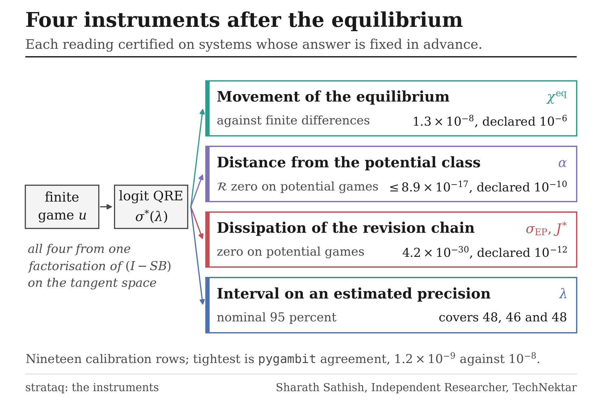
strataqis an open-source Python library, built on JAX, for logit quantal response equilibriumanalysis and for four capabilities that are routinely wanted after an equilibrium and thata dated prior-art sweep found unpackaged: the exact derivative of the equilibrium withrespect to payoffs, available in closed form as the strategic resolvent χeq = (I−SB)−1S onthe tangent space; the potential/harmonic decomposition of a finite game and its harmonicfraction α; the entropy production and stationary currents of the joint-profile revision chain,together with trajectory estimators calibrated against that exact meter; and a panel-awareestimation workflow whose interval names its own method.The paper states what each function computes, then reports the evidence that eachreading is correct on systems whose answer is fixed in advance by an analytic identity or byan external implementation. Nineteen calibration rows are reported: fifteen carry a declaredtolerance, fourteen a sample size and seventeen a committed artifact, and every exceptionis named in the tables. Most margins are wide because most rows are machine-precisionidentities, where the tolerance is a floor against catastrophic error. The row whose declaredtolerance actually constrains is the agreement with pygambit’s homotopy, at 1.2 ×10⁻⁹against a declared 10−8. The release-integrity failure in which twenty-three in-repositorygates were green while every solver call in the shipped wheel raised FileNotFoundError isreported as a failure mode with its diagnostic and its mitigation.
Keywords:
uantal response equilibrium
; logit equilibrium
; comparative statics
; potential games
; Hodge decomposition
; entropy production
; thermodynamic uncertainty relation
; research software
; JAX
1. Introduction
Quantal response equilibrium (McKelvey and Palfrey, 1995,9) is the standard structural model of noisy strategic choice, and its logit specialisation is the form almost all applied work uses: each player best-responds to expected payoffs with a precision parameter controlling how sharply the response concentrates on the best action. The model has a long descriptive record on laboratory games (Goeree and Holt, 2001; Goeree et al., 2016), an information-theoretic foundation in which is the inverse shadow price of Shannon information (Matějka and McKay, 2015), a decision-theoretic characterisation as the maximiser of expected payoff plus a scaled entropy (Fudenberg et al., 2015), and a statistical-mechanical reading in which the logit revision process on a potential game is a reversible Markov chain with a Gibbs stationary law (Blume, 1993; Brock and Durlauf, 2001).
Computing a logit equilibrium is a solved problem. The reference implementation is Gambit (Savani and Turocy, 2026), whose logit tracing homotopy (Turocy, 2005) is the production tool for following the correspondence from the centroid to the limit. strataq does not compete on that computation and validates against it (Section 8). The library exists because of what happens next. Once an equilibrium is in hand, four questions are asked routinely, and each of them is currently answered by code that is written afresh in every project that needs it.
Capability one: the movement of the equilibrium.
The object wanted is , the derivative of the equilibrium profile with respect to a payoff perturbation h. Solvers return the equilibrium and stop, so comparative statics are obtained by finite-differencing a re-solved equilibrium. That is slow, it is noisy at the tolerance the solver was run to, and near a turning point of the correspondence the re-solve can land on a different branch, in which case the difference quotient reports a large number that is not a derivative of anything. The derivative is available in closed form. Total differentiation of the logit fixed point on the tangent space gives the strategic resolvent (Appendix A), and the same factorisation supplies a uniqueness certificate through , a criticality warning as , and the vector-Jacobian product needed to differentiate an objective through the solve.
Capability two: distance from the potential class.
Candogan et al. (2011) give an orthogonal decomposition of a finite game into potential, harmonic and non-strategic flows, so that a single scalar, the harmonic fraction , measures how far a game sits from the potential class. That scalar is the natural independent variable for a great many questions about strategic structure, and the prior-art sweep recorded for this project (Section 2) located no packaged implementation of the decomposition on the indices it searched.
Capability three: dissipation of the revision process.
Logit revision on a finite game induces a continuous-time Markov chain on the joint profile space. That chain has a stationary distribution, stationary probability currents, and a Schnakenberg entropy production rate (Esposito and Van den Broeck, 2010b; Schnakenberg, 1976) which is exactly zero when the game is an exact potential game and positive otherwise. Time-series irreversibility tooling operates on a scalar series and has no representation of an agent, an action or a profile, so it cannot attribute dissipation to a player. Prior application of entropy-production ideas to social interaction data exists (Xu and Wang, 2011), and the review literature on coarse-grained bounds (Seifert, 2012,2) states the estimators, but the construction of the generator from a payoff tensor is what a game theorist needs and it is not packaged.
Capability four: the interval on an estimated precision.
Bland and Turocy (2026) wrote a manual for quantal response equilibrium estimation. The existence of a manual is itself the observation: the workflow is documented because it is not in the software. The reference estimation entry point returns a point estimate, a profile and a log-likelihood, and its input is a profile of aggregated counts, so subject, round and treatment identity are discarded before the likelihood is written down. Every published interval on is therefore hand-built, and intervals built differently in different laboratories are not comparable across papers.
Audience.
The intended users are experimental and behavioural economists fitting to laboratory or field data (Bland and Turocy, 2026; Haile et al., 2008); empirical industrial-organisation researchers testing conduct hypotheses where the equilibrium concept itself is part of the model (Calvano et al., 2020; Duarte et al., 2024); transport and network researchers for whom logit route choice is stochastic user equilibrium (Fisk, 1980); and researchers in statistical physics and econophysics who read strategic interaction through response functions and entropy production (Garnier-Brun et al., 2023; Scharfenaker and Foley, 2017).
1.1. Contributions
- C1.
- Response instruments as functions. The partial and equilibrium susceptibilities, the reciprocity defect built from the asymmetry of the latter, the strategic spectrum and the critical precision are exposed as callables computed from one factorisation of on the tangent space (Section 5). The equilibrium susceptibility is verified against central finite differences and against an independent implicit-differentiation path (Section 8).
- C2.
- Game geometry as a coordinate. The potential/harmonic decomposition (Candogan et al., 2011) and its harmonic fraction are computed on the normalised game (Section 5.3), together with a constructor that builds families of games at an exact target (Section 4), which turns a sweep over strategic structure into a controlled experiment.
- C3.
- Dissipation of the revision chain. The joint-profile Glauber generator, its stationary law, its currents and its exact Schnakenberg entropy production are constructed from the payoff tensor, and two trajectory estimators are calibrated against that exact meter with their bias directions and their failure modes measured (Section 9).
- C4.
- Calibration and validation. Nineteen readings on systems whose correct value is fixed in advance, reported with their declared tolerances, samples, registration status and artifacts, and with every gap in those columns named where it occurs (Section 7); four of them are separated out because an external implementation or a theorem proved elsewhere decides them (Section 8).
- C5.
- Reproducibility artifacts. The pre-registration discipline, the five-dimension gate, the isolated adversarial review, the regeneration entry point, the failure-mode table covering the packaging boundary and the release-integrity failure that produced it, and a provenance map from every figure, table and headline number to the artifact it came from (Section 10 and Appendix E).
1.2. Structure of the Paper
Section 2 places the library against pygambit, nashpy, OpenSpiel and QuantEcon on a capability matrix and states the search protocol behind the gap claims. Section 3 describes the three engines, the shared core, the enforced import boundary and the plugin contract. Section 4 gives the module and application-programming-interface map, the notation, and two worked calls with their printed output. Section 5 states the mathematics of the instruments and pushes the two derivations to Appendix A and Appendix B. Section 6 states the numerical discipline that the readings depend on, including the payoff-scale fold identity inherited from Sathish (2026c). Section 7 reports the calibration table and the margin figure. Section 8 reports the four rows decided by an external oracle. Section 9 reports the trajectory estimator calibration, its bias floor, its data-hunger failure and the distinction between the point estimate and the certified bound. Section 10 describes the evidence pipeline, the gate, the failure modes and the release-integrity failure. Section 11 states installation, dependencies, platforms, licensing, versioning, testing and the archival plan. Section 12 lists the known gaps, each with a remedy or a named next step, and Section 13 concludes. Appendix C records the tolerance ladder and the per-row registration status, Appendix D records the out-of-tree release check in full, and Appendix E maps every exhibit to its artifact.
2. Related Software and the Capability Gap
Four Python packages are the relevant comparison set. pygambit is the Python interface to Gambit (Savani and Turocy, 2026), the reference computational game theory suite, and carries the logit tracing homotopy of Turocy (2005) for both strategic and extensive form. nashpy (Knight and Campbell, 2018) computes Nash equilibria of two-player games by support enumeration, vertex enumeration and the Lemke–Howson algorithm. OpenSpiel (Lanctot et al., 2019) is a reinforcement learning framework for games, and includes magnetic mirror descent (Sokota et al., 2023), which converges to a quantal response equilibrium of a two-player zero-sum game at one fixed regularisation level. QuantEcon (QuantEcon Developers, 2024) supplies general finite Markov chain machinery, including stationary distributions and simulation, and game-theoretic routines for normal-form games, but no quantal response solver and no construction of a revision chain from a payoff tensor.
Table 1 sets the five packages against nine capabilities. The comparison is deliberately narrow: it asks only whether a capability is available to a user of the released package without writing the method, and it does not compare speed, breadth of equilibrium concepts, or maturity, on all three of which Gambit is ahead.
Reading the qualified cells.
OpenSpiel is marked partial on the first row because magnetic mirror descent returns the equilibrium of an entropy-regularised game at a fixed regularisation weight, which is a point on the quantal response correspondence and not the correspondence, and because the setting is two-player zero-sum. QuantEcon is marked partial on entropy production because it supplies the Markov chain object and its stationary distribution, on which a Schnakenberg rate could be assembled by the user, but neither the generator construction from payoffs nor the rate itself is provided. pygambit is marked partial on panel-aware estimation because its estimation entry point does return a maximum-likelihood point estimate and a log-likelihood, which is the hard part, but no standard error, no interval and no likelihood-ratio test, and it consumes aggregated counts. The last row records distribution model, never quality: nashpy and QuantEcon are pure Python; strataq ships a pure Python wheel on top of JAX (Bradbury et al., 2018) with no compiled extension of its own; OpenSpiel and Gambit both carry substantial C++, so a platform without a published binary wheel builds from source. The distribution facts in that row were taken from the project’s own packaging notes and were not re-verified against the package indices for this paper, so the row should be read as a statement about each project’s build model, never as a claim about any particular release.
Search protocol behind the gap claims.
An earlier draft of this paper asserted that no package on any index implements the Candogan decomposition. That assertion is not defensible as written, because a universal negative over unnamed indices cannot be checked. What the project can support is narrower and is stated here in that narrower form. A prior-art sweep was run on 8 August 2026 and is recorded in the repository at memory/literature-nearest-live-work.md, which names the sources it covered and the queries it used. That sweep located no packaged implementation of the Candogan decomposition, no solver exposing the equilibrium derivative in closed form, and no irreversibility estimator with an agent-and-profile data model. It located one-off notebook implementations of the decomposition associated with individual papers, and it confirmed that the nearest live game theory work on game decompositions (Legacci et al., 2024) does not release a package. No fresh sweep was run for this manuscript, so every gap claim in this paper is dated to 8 August 2026 and is a statement about what that sweep found, not about what exists. A reader who locates a packaged implementation later should treat the corresponding claim as superseded.
One terminological caution.
Legacci et al. (2024) decompose finite games into a potential and an incompressible part in order to study convergence and recurrence under exponential weights. Their incompressible component is defined by the vanishing divergence of a deterministic flow, while the harmonic component used here is the Candogan orthogonal complement of the potential subspace and is read through the dissipation of a stochastic revision chain; the two are different objects and the coincidence of the informal word “rotational” across the two literatures should not be read as an identity. This caution is repeated wherever that work is cited.
What each gap costs.
The absence of the equilibrium derivative costs accuracy and silence about its loss. A finite-difference comparative static inherits the solver tolerance in its numerator and divides by a small step, so its accuracy is bounded below by the solve accuracy divided by the step size, and there is no diagnostic in the output that says the two solves landed on different branches of the correspondence. The absence of the decomposition costs comparability: without , “far from a potential game” is asserted qualitatively for each game separately, and results obtained on one family of games cannot be placed against results obtained on another. The absence of an agent-aware dissipation meter costs attribution: a scalar irreversibility verdict on an aggregate series answers whether the series is time-reversible, and not which player’s response asymmetry generates the circulation, which is the version of the question a regulator or a mechanism designer can act on. The absence of a packaged estimation interval costs cross-paper comparison: each laboratory’s hand-built interval encodes its own resampling unit, and an interval that resamples observations where the design clusters within subject understates its own width. strataq closes the four by exposing them as functions with declared tolerances and committed calibration artifacts, which is the claim the rest of this paper supplies evidence for.
3. Architecture
strataq is a workspace monorepo whose importable package sits at packages/strataq. The architecture has three parts: three engines that do not share response operators, one core of machinery that all engines use, and a plugin contract under which application domains are added without touching either.
3.1. Three Engines, and What May Cross between Them
An engine is a representation of a strategic system together with the response and decomposition operators that representation admits.
- finite/
- The finite N-player strategic form. Dense payoff tensors, normalisation, the block susceptibility , the externality matrix B, the resolvent , the Hodge decomposition on the Cartesian-product graph of profiles (Candogan et al., 2011), the solvers and the exact revision dynamics.
- population/
- A continuum of agents with a payoff field . Potentiality is the symmetry of , and the logit equilibrium is Fisk’s stochastic user equilibrium with the Beckmann potential (Fisk, 1980; Sandholm, 2010).
- bayesian/
- Types and interim beliefs. This engine is deferred by an explicit recorded decision and is not started. The finite strategic-form machinery does not carry over as written, and beginning the engine requires an architecture decision record before any code lands.
The rule about crossing is enforced mechanically: only the response operators and the decomposition differ by engine, so everything else, meaning solvers, implicit differentiation, entropy utilities, dynamics construction and the typed configuration schemas, lives in core/ and is shared. An engine may depend on core/. core/ depends on no engine. No engine imports another engine. Figure 1 draws the layering with the boundary that a commit hook and a continuous-integration check both enforce.
3.2. The Plugin Contract
A domain is a plugin if and only if it declares exactly five objects together with an engine tag, and touches no core code. The five are specified as protocols in strataq/core/protocols.py:
- oracle
- a payoff oracle mapping an action profile to the vector of player payoffs;
- grid
- an action-grid builder turning the domain’s natural continuous or combinatorial choice set into a finite action set;
- field
- a ConjugateFieldSpec naming the observable payoff perturbation with respect to which the response instruments differentiate, such as a link toll, an allocation budget, or a wholesale cost;
- loader
- a dataset loader producing the domain’s data in the shape the oracle expects;
- learn
- a documentation page stating what the domain is and what its readings mean.
The ConjugateFieldSpec is mandatory, which is the part of the contract that does work. A domain in which no observable payoff perturbation can be named declares NONE, and the response instruments then refuse to run. They do not return a number computed against an unobservable perturbation. Figure 2 draws the contract and the consequence of the absent field specification. The design invariant behind the whole contract is that a domain requiring core machinery it does not have is an engine, whatever it is called, and adding an engine requires a recorded decision first.
3.3. Two Surfaces over One Machinery
The library presents two surfaces. The lower one is the instrument layer, whose callables take payoff tensors and precisions and return readings: logit_qre, chi_equilibrium, reciprocity_defect, alpha, hodge_decompose, and the dynamics and estimator entry points. The upper one is strataq.problems, which takes a domain-shaped problem statement, such as a set of costs and a price grid, and returns a frozen solution object with domain-named fields, a printable summary and a .diagnostics attribute holding the instrument readings computed lazily. The upper surface calls the lower and never reimplements it, and the facade’s numbers are checked against the research artifacts they claim to reproduce. That check is what caught the release-integrity failure of Section 10.
4. What the Library Computes
This section is a map of the public surface. Table 2 fixes notation for the rest of the paper, Table 3 lists the modules with their principal callables and their gate status, and the two listings that follow show the library being used.
Solvers.
logit_qre is a just-in-time compiled damped Krasnosel’skii–Mann iteration (Krasnosel’skii, 1955; Mann, 1953) on the logit fixed point. mirror adds magnetic mirror descent (Sokota et al., 2023), a structurally different last-iterate-convergent method, so that solver dependence of a reading is a testable proposition; the two are required to agree, and their agreement is a calibration row. homotopy is a pseudo-arclength branch tracer along the correspondence, with fold detection by reversal of the direction of and recorded at every step, so a turning point is a labelled event in the output. implicit differentiates through the fixed point with a custom vector-Jacobian product on the transposed tangent system, and shares the factorisation with the response instruments.
Constructing families at a target geometry.
make_family builds games at an exact target harmonic fraction. The consequence is methodological: without such a constructor, an experiment across strategic structure is a survey of whatever games are convenient and is a measured covariate, whereas with it is an assigned treatment and the sweep is a designed experiment.
Repeated, evolutionary and extensive modules.
repeated represents strategies as Moore machines, so grim trigger and tit-for-tat are data, with no separate code path for each, and answers the two folk-theorem questions, sustainability at a discount factor and the critical discount factor, in closed form for grim trigger and by one-shot deviation generically; it adds a logit analogue in which sustainability is a probability, and measures Edgeworth cycles (Maskin and Tirole, 1988) from alternating logit best response on a price ladder. evolutionary carries replicator dynamics in continuous and discrete time, rest points by support enumeration classified by tangent-space eigenvalues, the logit dynamic whose rest points are the logit equilibria, and the finite-population Moran process. The two selection formalisms meet at one scalar, because the selection intensity of the Fermi rule is the logit precision, and compare_intensity reports both readings together with the gap between them. extensive stores trees as flat preorder arrays with a nested-dictionary constructor that doubles as the on-disk format, and implements the two tree passes, the reduced normal form, Kuhn’s theorem (Kuhn, 1953), backward induction, a catalogue of classic trees, and the agent quantal response equilibrium (McKelvey and Palfrey, 1998) on the same damped fixed point as the strategic-form solver.
Problems, verdicts and refusals.
Five problem types share one contract of construct, solve and summarise: PricingProblem, AuctionProblem, RoutingProblem, AllocationProblem and ElectricityProblem. Problems validate on construction and raise errors naming the offending field. Solutions are frozen dataclasses with domain-named fields, a printable summary, and a .diagnostics attribute carrying the response, decomposition and dissipation readings, computed only when requested. solve_situation assembles a recommendation together with a sensitivity block that re-solves across a ladder of precisions and reports the fraction of the ladder that agrees and the precision at which the recommendation first changes, so a recommendation that holds from to is distinguishable in the returned object from one that holds only at the precision supplied. diagnose is the single-call entry point returning a verdict together with .explain() for every band, null, warning and refusal behind it, .snippet() for runnable code reproducing exactly that reading, and .plot() for the point in the response-asymmetry against dissipation plane. Refusal is a return value throughout: a flat likelihood is reported by fit as the interval it is, namely the whole search window, with the point estimate withheld; an unidentifiable coordinate is reported by diagnose as a bound or as a named pair of regions it cannot separate.
4.1. Two Calls with Their Output
Two listings follow. Each is complete, so no appendix repeats them. The first states a two-firm pricing problem on a nine-level price grid with logit demand, solves it, and prints the summary table. The printed block is the output of the call.
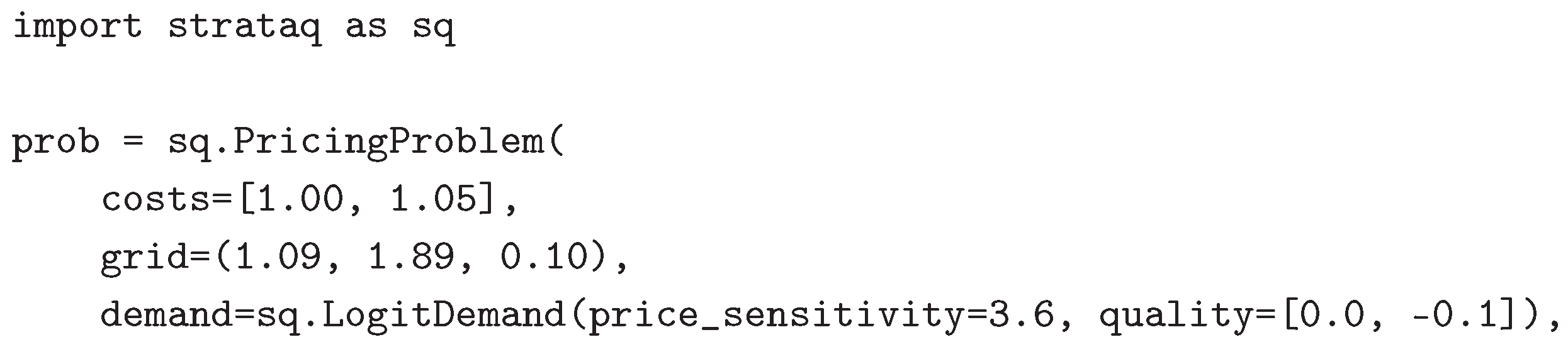
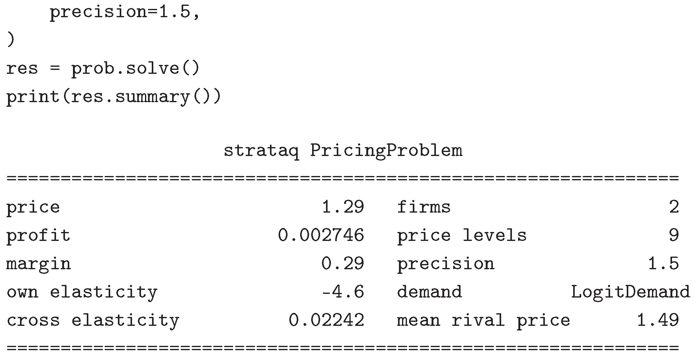
The returned object carries res.price as the price to set, res.rival_prices as the distribution over each rival’s price, res.profit_curve as the profit at every grid level, and res.elasticities as the own and cross elasticities there. The same three lines run on real network data: sq.RoutingProblem(network="sioux_falls", tolls={28: 5.0}).solve() returns link flows on the 76-link network, the total travel time, and a toll_effect block with the revenue collected and the change in flows.
The second listing asks the diagnostic question instead. It takes a game, here rock-paper-scissors, and returns a verdict located in the plane of response asymmetry against dissipation.
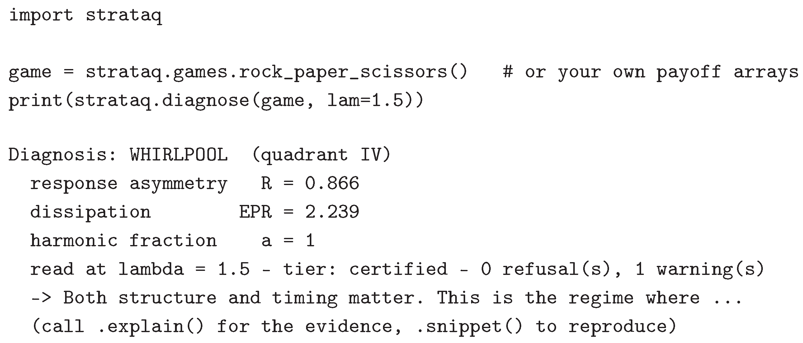
The console uses plain ASCII names for the symbols of Table 2: the printed R is the reciprocity defect , EPR is , and a is the harmonic fraction . The advisory line is reproduced here as the repository documentation publishes it, with the sentence cut short; the call prints it in full.
Four things in that output are design of the surface, not incidental formatting. The precision at which the reading was taken is printed on the same line as the reading, because the magnitude of is precision-dependent (Section 5). The confidence tier is printed, so a certified reading and a diagnostic reading are not typographically identical. The refusal and warning counts are printed even when they are zero, so their absence is an observation. And the harmonic fraction is printed beside the two readings it organises, which is what makes the verdict a location. The dissipation value printed here is the exact Schnakenberg rate for this game at this precision, and it recurs in Section 9.2 as the ground truth against which the trajectory estimator is scored.
5. The Instruments
This section states what the instruments compute. The two derivations that a reader may want to check are in Appendix A and Appendix B.
5.1. The Logit Fixed Point and the Two Susceptibilities
Write for the expected payoff to player i of action a against the opponents’ profile. A logit quantal response equilibrium at precision vector is a profile satisfying
where is an additive perturbation of player i’s payoff vector, zero at the reference configuration, supplying the direction along which the response instruments differentiate. This is the entropy-regularised best response, that is, the maximiser of expected payoff plus times the Shannon entropy of (Fudenberg et al., 2015; Matějka and McKay, 2015). Numerically it is always evaluated through log_softmax and logsumexp, never by exponentiating raw payoffs.
Differentiating the softmax gives the partial susceptibility, the response of a player to a payoff shock with opponents held fixed:
which is the static fluctuation-dissipation statement for an exponential family, being the covariance of the action indicator under . Collecting the blocks gives .
Holding opponents fixed is not what happens in equilibrium. Total differentiation of Equation (1) in h, carried out on the tangent space in Appendix A, gives the equilibrium susceptibility
with the externality matrix. The Neumann expansion reads Equation (2) as the direct response S plus every path of strategic feedback through opponents, and converges exactly when . The relation of to a response matrix in economics is the same relation that connects a Slutsky matrix to a susceptibility (Garnier-Brun et al., 2023): the symmetry of the matrix, not its size, is the structural statement.
Figure 3 draws the consequence for the implementation. The same factorisation supplies the comparative static, the uniqueness certificate and the reverse-mode gradient, so the three cannot report inconsistent conditioning. When approaches one the instruments issue a criticality warning instead of returning a large silently, because near a fold the magnitude is dominated by the conditioning of the resolvent and only the direction of the response remains informative.
5.2. The Reciprocity Defect
The reciprocity defect is the normalised antisymmetric part of the equilibrium susceptibility,
It answers a question with an operational form: if a shock to player j’s payoff moves player i’s equilibrium behaviour by a different amount than the mirror-image shock to i moves j, the system is not describable by any single scalar objective that all players are climbing. Appendix B shows that exactly when the normalised game is a potential game, by way of the identity , whose middle factor vanishes precisely when on .
The equivalence between symmetry of the externality structure and potentiality is not a contribution of this work. It is the standard characterisation of potential games (Monderer and Shapley, 1996), in the form given for population games by Sandholm (2010) and for differentiable games by Balduzzi et al. (2018), with the flow-decomposition version supplied by Candogan et al. (2011) and the statistical-mechanical reading by Blume (1993). What the library adds is that the characterisation is evaluated through the equilibrium response matrix, which is an object an experimenter can estimate from observed cross-agent pass-through without knowing the payoff tensor.
Two properties are documented at the call site because both are easy to misread, and one of them was misread in an earlier internal draft of this project.
is a ratio of norms and is not bounded above by one.
The denominator is the norm of the symmetric part, not the norm of , so exceeds one whenever the antisymmetric part is larger than the symmetric part in Frobenius norm. Matching pennies reads . Reporting as a percentage or as a fraction of a whole is therefore wrong.
Only the zero of is precision-free.
Whether does not depend on , because S is invertible on for and full-support , so the vanishing of the middle factor is a statement about B alone. The magnitude of does depend on , because both norms in Equation (3) scale with S and with the resolvent. Any reported level of therefore carries the precision it was read at, and levels read at different precisions are not comparable. This is enforced by the reporting format shown in Section 4.1.
5.3. The Harmonic Fraction
Candogan et al. (2011) decompose the space of finite games, viewed as flows on the Cartesian-product graph of pure profiles, into three orthogonal subspaces: potential, harmonic and non-strategic. The non-strategic component does not affect the quantal response equilibrium at any precision, so the informative coordinate is the split of the strategic part. The library computes
on the normalised game, using a separable Kronecker form of the projection so that the transform never materialises the full profile-graph incidence operator. Normalising first is not cosmetic. Full externality symmetry is sufficient but not necessary for potentiality of the raw game, so a decomposition applied to the raw tensor can report a harmonic component that a change of the non-strategic part removes (Legacci et al., 2024, Lemma C.2 and Example C.2). Decomposing the normalised game is the standing rule.
That reference carries a terminological collision, repeated here because it is repeated wherever the work is cited: the incompressible component of Legacci et al. (2024) is defined by the vanishing divergence of a deterministic flow, whereas the harmonic component here is the Candogan orthogonal complement of the potential subspace and is read through the dissipation of a stochastic revision chain. The two constructions answer different questions and should not be identified.
5.4. Entropy Production of the Revision Chain
Logit revision induces a continuous-time Markov chain on the joint profile space. In the Glauber form each player revises at a fixed rate and, when revising, draws a new action from the logit response to the current opponents’ profile, so the generator L has non-zero entries only between profiles differing in one player’s coordinate. Let be its stationary law. The Schnakenberg entropy production rate (Esposito and Van den Broeck, 2010b; Schnakenberg, 1976) is
with the stationary currents . On an exact potential game the chain is reversible with (Blume, 1993; Monderer and Shapley, 1996), every current vanishes and Equation (4) is exactly zero. Away from that class the currents circulate and the rate is positive. The generator, its stationary law, its currents and Equation (4) are computed exactly for small games, which is what makes the trajectory estimators of Section 9 calibratable at all: a bound is only useful when there is a system on which the quantity it bounds is known.
The library also implements the Hatano–Sasa split of the total rate into housekeeping and excess parts, (Esposito and Van den Broeck, 2010a; Hatano and Sasa, 2001), together with stepwise quench protocols in and their integral fluctuation theorems (Crooks, 1999; Jarzynski, 1997). Those readings are the subject of Sathish (2026c) and are used here only as calibration rows (Section 7), where the fluctuation theorems supply identities that must hold at machine precision.
Spectral reality and the absence of oscillation.
On a full potential game, implies that is similar to the symmetric matrix , so its spectrum is real and no complex pair can cross the imaginary axis. Logit dynamics on such a game therefore cannot undergo a Hopf bifurcation. The contrapositive is visible in the literature: Hommes and Ochea (2012) exhibit limit cycles under logit dynamics on rock-paper-scissors, which is at the harmonic extreme. The library records the spectrum along every homotopy branch, and the reality check is a calibration row.
5.5. Trajectory Estimators
Data never supplies a generator. It supplies a sequence of observed profiles. Two estimators bridge the gap and are stated here, with their calibration reported in full in Section 9. The first is the k-block Kullback–Leibler estimator of Roldán and Parrondo (2010), which compares the law of forward -blocks with the law of their reversals. The second is the finite-time thermodynamic uncertainty relation (Barato and Seifert, 2015; Horowitz and Gingrich, 2017), which lower-bounds the rate by for any time-integrated current , and therefore returns a certified bound (Otsubo et al., 2022). Surrogate null classes for observational data, including phase-randomised and amplitude-adjusted surrogates (Schreiber and Schmitz, 1996; Theiler et al., 1992) and a reversibilised-Markov null matching an observed chain’s persistence, live in thermo.nulls.
A priority statement.
That a local response asymmetry and a global dissipation functional are inequivalent objects is established for Markov jump processes and is not claimed here. Baiesi et al. (2009) show that the response of a non-equilibrium state splits into an entropic and a frenetic term, so response is not a functional of entropy production alone; and the neighbouring Langevin statement runs the other way, since Harada and Sasa (2005) show that there the integrated violation of the fluctuation-response relation equals the dissipation. What this library contributes on that axis is the instantiation on finite strategic-form games, the explicit Hodge coordinate that organises it, and the measurement; the measurement itself is reported in Sathish (2026b) and is not restated here.
6. Numerical Discipline
The readings of Section 5 are only as good as the arithmetic under them. Five rules are enforced across the library, and each exists because violating it produces a specific wrong answer whose signature is stated with the rule.
Float64, always.
JAX defaults to single precision. The library enables 64-bit arithmetic at import. This is a correctness requirement and not a preference, because is near-singular exactly where the interesting behaviour is. Near a fold the resolvent amplifies the representation error of its own entries, and at single precision the amplified error reaches the leading digits of before the criticality warning fires. All linear algebra in the library is float64, and the calibration rows at and below in Table 5 would be unreachable without it.
The tangent space, and what skipping it manufactures.
The curvature block satisfies by construction, so is rank-deficient and S carries one exact null direction per player. Those null directions are not features of the game; they are the statement that a mixed strategy sums to one. If the resolvent algebra is run on the full simplex coordinates, therefore inherits eigenvalues at exactly one from the constraint directions, and reports a value of one at every configuration. Since is the criticality signal, running on the wrong space manufactures a false criticality reading everywhere, and the instrument that is supposed to warn about folds becomes a constant. All algebra therefore runs on .
The Helmert basis.
The projection onto is realised through an explicit orthonormal basis in place of pseudo-inversion, because an explicit basis makes the reduced operator exactly -dimensional and its spectrum exactly free of the constraint directions, whereas a pseudo-inverse leaves a numerical zero that has to be thresholded, which reintroduces a tuning constant into the criticality test. The basis used is the Helmert contrast basis (Lancaster, 1965), whose r-th row is proportional to with r leading ones, normalised. Its columns are orthonormal, its construction is closed-form at any , and it is the same basis in every module, so a spectrum computed by the response instruments and a spectrum recorded by the homotopy tracer are computed in identical coordinates. The construction is given in Appendix A.
The tolerance ladder.
No numerical literal appears in library code. Tolerances, seeds, grids and precision ranges are read from a typed configuration schema, and every tolerance sits on the four-level ladder of Table 4. The ladder exists so that the requirement a check must meet is determined by the kind of comparison being made, never by the number that came out of it.
Explicit pseudorandom keys.
Every stochastic call site takes an explicit key folded from a root recorded in the resolved configuration snapshot written beside each artifact. There is no global generator and no implicit seeding. The consequence used throughout Section 7 is that a row regenerates bit-for-bit from the artifact’s own record, so a rerun that differs is a code change, never a sampling accident.
Normalised precision, and the payoff-scale fold.
Payoffs are rescaled internally before decomposition and before the response algebra. The scale does not disappear: it folds exactly into the precision. For any reading the library computes, and any payoff tensor u and scale ,
an algebraic identity that follows from the fact that and u enter Equation (1) only through the product . It is checked numerically to error in the work reported by Sathish (2026c), where it is used to establish that a feature located in the plane is physical only in the normalised coordinate. The operational consequence for this library is a reporting rule: every reading reports the raw precision and the normalised precision , because Equation (5) means that a comparison of two systems at equal but different payoff scale is a comparison at different effective precision. That confound has caught one experiment in this project’s own record, and the two-column reporting exists so that it cannot recur silently.
7. Calibration
Calibration here means measurement on systems whose correct reading is fixed in advance by an analytic identity or by an external implementation. Table 5 and Table 6 list nineteen such systems between them, each with the requirement it had to meet, the sample it was taken on, whether that requirement was registered before the run, the value measured, and the artifact it regenerates into. Those columns are not complete, and the gaps are visible in the tables rather than smoothed over: fifteen of the nineteen rows carry a declared numeric or directional requirement, fourteen carry a sample size, and seventeen carry a committed artifact. The seventeen committed artifacts regenerate from seed 20260808 under make reproduce and are JSON records carrying metrics, effect sizes with intervals where the quantity has a sampling distribution, the sample size, a justification of that size, the seed, the configuration reference and the library version. The remaining two rows are the log-partition identity, which is checked in the test suite and writes no artifact, and the quench fluctuation theorems, whose unit is named but whose artifact filename this manuscript’s evidence base does not record.
What the registration column records, and what it does not.
Section 10 describes a discipline in which the acceptance criterion is written into a configuration file and committed before the experiment runs, and in which a gate written after the measurement as a regression contract says so in its own header. That per-row status exists in the gate files. It was not extracted into this paper’s evidence base, so seventeen of the nineteen registration cells in Table 5 and Table 6 are marked nr, and their registration status is unverified from this document alone. Appendix C states the extraction procedure, which is a single pass over the gate headers, and records that it is the largest gap between what the repository knows and what this paper reports. Two rows are marked post because the project record states directly that they are regression contracts: the Blotto degenerate null was found while writing the positive test and kept as a regression, and the requirement that the thermodynamic uncertainty bound sit below the exact rate was made a test after the failure described in Section 9.

Table 5.
Calibration, part one: rows on which a theorem or a closed-form identity fixes the correct value. n is the extent of the check in the units the row is replicated over, which differ by row; a dash means the row is a single evaluation with no replication. Reg. records whether the requirement was registered before the run: nr means the status is in the gate file and was not extracted (Appendix C), post means the requirement was written after the measurement as a regression contract.
Table 5.
Calibration, part one: rows on which a theorem or a closed-form identity fixes the correct value. n is the extent of the check in the units the row is replicated over, which differ by row; a dash means the row is a single evaluation with no replication. Reg. records whether the requirement was registered before the run: nr means the status is in the gate file and was not extracted (Appendix C), post means the requirement was written after the measurement as a regression contract.
| Reading | Req. | n | Reg. | Measured | Artifact |
|---|---|---|---|---|---|
| , | – | nr | holds; no scalar recorded | test suite; no committed artifact | |
| Gibbs on congestion, | 2 sizes | nr | gibbs_agreement | ||
| and on exact potential games | 5 games | nr | ; | equilibrium_reads_zero | |
| on exact potential games | 5 games | nr | reciprocity_potential | ||
| on RPS-3, RPS-5, matching pennies | 3 games | nr | , , | reciprocity_harmonic | |
| Spectrum of real on potential games, | rel. imag. | 5 games | nr | 0; harmonic contrast | spectrum_reality |
| Population engine: Beckmann gradient equals route costs; toll against finite differences | ; | – | nr | 0; | population_identities |
| Sioux Falls: , defect, Fisk conditions | ; ; | 76 links, 8 pairs | nr | ; 0; | sioux_falls_calibration |
| Blotto: and at | not declared | 1 instance | nr | ; | blotto_readings |
| Blotto degenerate constant-payoff null | not declared | 1 instance | post | blotto_readings | |
| Quench fluctuation theorems, Jarzynski and Hatano–Sasa | machine precision | – | nr | holds; no scalar recorded | unit thermo.protocols; filename not recorded |
Why most margins are enormous, and the one row where the tolerance bites.
Figure 4 shows most rows sitting four to seventeen decades below their declared requirement. That is not evidence of severe testing and should not be read as such. Most of these rows are machine-precision identities: a quantity that a theorem says is exactly zero is computed, and the only achievable values are zero and rounding noise. For those rows the declared tolerance is a floor against catastrophic error, meaning a projection applied on the wrong space, a sign convention inverted, a matrix transposed, or a solve run at single precision, all of which produce residuals many orders above and not slightly above it. A tolerance of that kind discriminates between correct and grossly wrong, and carries no information about how nearly correct the code is. Two rows are different in kind, and both are comparisons against something that is not an identity. The pygambit agreement row measures against a declared , a margin of a factor of , and it is the tightest row in the table: it constrains, and a modest regression in either implementation’s convergence criterion would breach it. The finite-difference row measures against a declared , a factor of 77, and its residual is dominated by the truncation of the difference quotient at the step size used, so it is a check on the closed form and not on the solver. The toll-susceptibility row against finite differences is next at a factor of 357. Everything else in the table is an identity check whose value lies in what it would catch, not in the size of its margin.
Table 6.
Calibration, part two: rows on which a second computation, an external implementation or a directional requirement fixes the correct value. Column conventions as in Table 5.
Table 6.
Calibration, part two: rows on which a second computation, an external implementation or a directional requirement fixes the correct value. Column conventions as in Table 5.
| Reading | Req. | n | Reg. | Measured | Artifact |
|---|---|---|---|---|---|
| against central finite differences | 50 games | nr | chi_fd_agreement | ||
| Implicit-differentiation product against the resolvent | 20 games | nr | implicit_chi_agreement | ||
| Mirror descent against damped solver, same fixed point | – | nr | solver_cross_agreement | ||
| pygambit fixed- agreement | 32 games × 2 | nr | gambit_agreement | ||
| Branch tracer through fixed- points | – | nr | branch_agreement | ||
| k-block KLD against the exact meter across | not declared | 10 levels | nr | Spearman ; per-level relative error of order | estimator_alpha_sweep |
| Debiased finite-time TUR bound below the exact rate | bound ≤ exact | 10 levels | post | holds at 10 of 10; median tightness | estimator_alpha_sweep |
| KLD on named ground-truth games | not declared | 2 games | nr | where the exact value is 0; against an exact | estimator_ground_truth |
Sample sizes and what fixes them.
The counts in Table 5 and Table 6 are small and their justification is structural. The identity rows use the number of distinct constructions available: five exact potential games spanning the constructions the library can build, three harmonic games at the extreme, two congestion sizes. Increasing those counts adds instances of the same identity and does not add discriminating power, because an identity either holds on a construction or it does not. The two rows with larger counts are the ones where the residual has a distribution: fifty random games for the finite-difference comparison and thirty-two seeded games at two precisions for the external oracle comparison, in both of which the reported number is a maximum over the sample, so a larger sample is a stronger claim. The estimator rows are sized by the sweep design, ten levels of , and their sampling behaviour is reported in Section 9. The per-row justification is recorded in each artifact’s own n_justification field.
7.1. The Potential Anchor: Congestion on Real Network Data
Congestion games (Rosenthal, 1973) are exact potential games, so every instrument has a known reading on them: the harmonic fraction is zero, the reciprocity defect is zero, the stationary currents vanish and the entropy production is zero. In the population form, logit route choice is Fisk’s stochastic user equilibrium (Fisk, 1980), whose convex potential, the Beckmann integral of the link cost functions plus a scaled entropy term, is known in closed form. Link costs use the standard Bureau of Public Roads form (Bureau of Public Roads, 1964).
On the Braess diamond the automatic-differentiation gradient of the Beckmann integral equals the route-cost vector exactly. That single identity composes the payoff oracle, the network representation, the potential and the differentiation machinery, so it is the end-to-end check with the widest coverage in the project. On the Sioux Falls network taken from the public TNTP record (Transportation Networks for Research Core Team, 2026), with 76 links, the top eight origin-destination pairs and shortest-path route sets, the Fisk conditions hold to , the symmetry defect of is exactly zero, the toll-response reciprocity defect reads and the toll susceptibility matches central finite differences to with the sign verified against actual re-solves.
The scope of that reading is the following. The route sets are k-shortest restrictions and the origin-destination set is a subset of the full matrix, so the computed link flows are not comparable with the repository’s best-known equilibrium flows for the full problem; the diagnostic gap of between them is reported as a diagnostic and never as a certificate of anything. The instrument identities are exact within the route set regardless of that restriction, which is what the row is asserting.
One engineering fact is recorded because it changes how the population engine is implemented: the damped logit-assignment map is not a contraction on networks with steep link-cost exponents. On the Braess diamond it enters a two-cycle. The stochastic user equilibrium is therefore obtained by damped Newton iteration on the convex program.
7.2. The Harmonic Anchor: Colonel Blotto
The other anchor needs a game with a non-zero harmonic component and an exactly observable conjugate field. Two-player Colonel Blotto over lattice-simplex allocation grids supplies both, because the budget is the field: it is a payoff perturbation an outside observer can name and vary. Three instances are reported. The symmetric instance with budget three over three fields reads and at . An asymmetric instance reads with visible circulation in the stationary currents. A degenerate instance with equal field values and budget two, in which every profile ties, has constant payoffs, and every meter reads zero, with . That null was found while writing the positive test and was kept as a regression row, which is why it carries the post registration mark.
One calibration result corrected an assumption the project had written down. Blotto is a mixed game and not a pure harmonic one: , well short of 1. Zero-sum does not imply harmonic-pure. Rock-paper-scissors, at exactly, remains the pure extreme, so the right-hand end of the bracket available from a realistic strategic system sits near and the pure extreme is reachable only from a constructed game.
7.3. The Dissipation Axis
The last three rows of Table 6, together with the fluctuation-theorem row of Table 5, calibrate the dissipation instruments against the exact meter of Equation (4): the trajectory estimators across a ten-level sweep in , the same estimators on two named ground-truth games, and the quench fluctuation theorems. Those rows carry enough methodological weight that they are reported in full in Section 9 instead of being summarised here. Two points belong with the tables themselves. First, the fluctuation-theorem row has no committed artifact filename in this paper’s evidence base, only a unit name and a findings-log identifier, which is recorded as such in Table 5 and in Appendix E. Second, the thermodynamic uncertainty row is a directional requirement, that the bound lie below the exact rate, so it does not appear in Figure 4.
8. Validation against Reference Implementations
Four of the calibration rows are separated out here because in them an external implementation, or a theorem proved elsewhere, decides whether the library is right. Table 7 states them together with the status of the evidence each produces, which is not the same in all four.
Against pygambit, strategic form.
pygambit implements the logit tracing homotopy of Turocy (2005), which follows the correspondence from the centroid. On 32 seeded games at two precisions each, the library’s fixed-precision profiles agree with it to a maximum profile gap of against a declared oracle tolerance of . The branch tracer is checked the same way but along the whole correspondence, and reproduces the direct solve at fixed-precision crossings to . pygambit is an optional test-time dependency and is never a run-time requirement, so the comparison converts the reference implementation from a competitor into a certificate. The value of the comparison is limited in one direction worth naming: agreement to establishes that the two implementations locate the same fixed point of the same correspondence, and does not establish that either is the fixed point a third implementation would find if both shared a common error in the definition of the expected-payoff map. The independent checks against finite differences and against the analytic potential exist because that limitation is real.
Against pygambit, extensive form.
The agent quantal response equilibrium (McKelvey and Palfrey, 1998) is compared with pygambit’s extensive-form logit solver on four classic trees: entry deterrence at , the four-stage centipede, Selten’s horse and Kuhn poker, with the maximum behaviour-strategy gap required to sit inside the oracle tolerance in each case.
This check does not produce evidence of the same standing as the other three, and the difference is stated at this point, because this is where the claim would otherwise be made. The comparison lives in the test suite and not in a committed benchmark artifact, and it is marked skipif(not HAVE_GAMBIT). pygambit is an optional dependency. A continuous-integration run in an environment without it therefore reports a passing extensive-form suite in which the only external check never executed, and nothing in the passing report distinguishes that case from one in which the check ran and passed. The consequence for a reader is direct: the extensive-form agreement should be treated as a developer-side check that has been observed to pass, and not as a reproducible artifact. It is deliberately absent from the abstract for that reason, and the remedy, promoting it to a committed benchmark artifact as the strategic-form comparison already is, is named in Section 12.
Against finite differences, and against a second derivative path.
That in Equation (2) is the derivative of the equilibrium is checked two independent ways. Central finite differences of the solved equilibrium under a payoff perturbation agree with the closed form to across 50 random games, against a declared finite-difference tolerance of . The residual at that level is consistent with truncation of the central difference quotient at the step size used, since the solve tolerance is far below it; that attribution is an inference from the tolerance ladder and has not been confirmed by a step-size sweep, which is the check that would settle it and which Section 12 records as not run. Independently, the implicit-differentiation vector-Jacobian product, which solves the transposed tangent system without ever forming the resolvent, reproduces the same matrix to on 20 games. Agreement at that level is the statement that the two code paths are the same mathematics and not merely close, since two different approximations of the same object would not agree to rounding.
Against an analytically known potential.
The population engine’s identities are exact, which is what makes them a check on the code itself. The automatic-differentiation gradient of the Beckmann integral equals the route-cost vector to exact zero; the symmetry defect of is exact zero; and the Fisk conditions hold to on the real network of Section 7.1. An instrument whose central reading is a potentiality test has to read zero where a theorem says zero, and this is the row where that is tested against someone else’s theorem.
9. Estimator Calibration
Everything in Section 5.4 used the generator. Data never supplies a generator: it supplies an observed sequence of profiles. This section reports the calibration of the two trajectory estimators against the exact meter, on synthetic trajectories, before any contact with observational data. The unit is thermo.estimators, and its gate was signed off after one blocking objection which is disclosed below because the correction it forced is part of the result.
9.1. Why the Skeleton Chain Is the Right Estimation Object
Simulation is by uniformisation: with , the skeleton chain is stepped with exponential holding times of rate . Two exact facts make the skeleton, in place of the continuous-time trajectory, the object the estimators consume. It shares the stationary law of the generator, so a statistic computed on skeleton steps is a statistic of the same stationary process. And its per-step entropy production is exactly , so a per-step estimate converts to a rate by one known factor with no discretisation bias. Together with the block identity of the next paragraph, this gives the estimator a sharp target at every block order rather than a target that has to be argued for.
9.2. The Block Target and Its Plug-In Bias Floor
For a stationary Markov chain the Kullback–Leibler divergence between the law of forward -blocks and the law of their reversals equals k times the per-step entropy production (Roldán and Parrondo, 2010). The plug-in estimator is
with the mean holding time. Across the ten-level family in at , with stationary steps per level, Equation (6) at recovers the exact Schnakenberg rate with Spearman rank correlation and a per-level relative error of order one percent.
Two failure directions are measured. On exact potential games, where the truth is zero, the plug-in estimator reads below where the truth is zero. That residual is the plug-in bias of a divergence estimated from finite counts, which is non-negative by construction, so the estimator has a floor and cannot certify the absence of dissipation. On the named ground-truth games the same estimator reads where the exact answer is zero and against an exact on rock-paper-scissors, which is the same reading that appears in the diagnose output of Section 4.1.
The second direction is data hunger. The block identity is a population statement, and the number of distinct -blocks grows as . When the sample is not much larger than that count the empirical block law is sparse, the estimated divergence is pulled towards its own support, and the estimator understates. At the validation sample size, reads about 17 percent low. The direction matters: an estimator that understates dissipation is conservative for a claim that dissipation is present and anti-conservative for a claim that it is absent. That failure mode is itself a regression test, so a future change that removes the underestimate without explanation will be caught.
9.3. The Thermodynamic Uncertainty Bound and Three Facts That Changed the Number
For any time-integrated current of a stationary continuous-time Markov chain, the finite-time thermodynamic uncertainty relation (Barato and Seifert, 2015; Horowitz and Gingrich, 2017) gives
This is a certified lower bound and not a point estimate. A poor choice of current loosens it and never breaks it, which is the property that makes it the designated headline quantity for partially observed data (Otsubo et al., 2022; Seifert, 2026). Three methodological facts were established adversarially during the calibration, each changed the number, and each is now a test. Table 8 states them.
What the certified statement therefore is.
The reportable quantity is the lower bootstrap quantile of Equation (7) over windows, and not the plug-in ratio. Across the ten sweep levels that quantile lay below the exact rate at every level, and it is the only quantity in this family that the library will describe as a bound. Window resampling uses the block bootstrap (Efron and Tibshirani, 1993; Künsch, 1989; Politis and Romano, 1994), since successive windows of a single trajectory are not independent.
The correction the adversarial review forced.
The first artifact written for this unit described the debiased point estimate as a certified bound. The red-team review blocked the gate and refused to accept a wording change, on the ground that a distinction which matters is one that the interface should make impossible to lose. The distinction was therefore made structural: the certified quantity is returned by a separate entry point, tur_epr_bound_ci, which returns the interval and its lower quantile, while the plug-in ratio is returned by a different call and is documented as an estimate. This is recorded here because the interface split is the durable part of the result, and because the artifact’s original language would otherwise have propagated into this paper.
Tightness read as a diagnostic.
The ratio of the bound to the exact rate is approximately at and drifts to to by , with a median across the sweep of . The bound is therefore tightest where the dissipation is smallest, which is where linear response saturates the relation, and loosest where there is most dissipation to measure. For a conservative instrument that is the correct failure direction: the degradation is graceful, it is monotone in the coordinate that organises the sweep, and the instrument never claims more than the truth. It also means that tightness itself carries information about the regime, so the library reports the ratio alongside the bound when the exact rate is available.
9.4. Estimating the Precision from Data
The estimation surface is calibrated separately, because its failure mode is misspecification. estimate.lam runs four structurally different estimators of : a frequency maximum-likelihood estimator with a profile-likelihood interval, an automatic-differentiation maximum-likelihood estimator through an unrolled solve, moment matching on , and inversion of the choice dispersion. On well-specified synthetic data the four are consistent, with a median relative error at or below 3 percent. On data generated from a mixture of precisions, which is the canonical misspecification for this model, the spread between the four widens by a factor of 91. That is the agreement protocol’s purpose: the disagreement between estimators is reported as a misspecification diagnostic, and an unidentified case produces a warning and a withheld point estimate.
estimate.bayes supplies a grid posterior with a self-diagnosing resolution guard, mixture Bayes factors, and an experiment-selection loop scoring candidate designs by expected information gain (Houlsby et al., 2011; Lindley, 1956). The interval it quotes was checked for coverage after a bug in which the interval was quantised to the grid: nominal 95 percent intervals cover at 48, 46 and 48 out of the replicates run at each of three true precisions. Coverage counts of this form are naturally summarised with a Wilson interval (Wilson, 1927); the artifact records the counts, and this paper does not convert them, because the replicate count per cell is recorded in the artifact, which this manuscript’s evidence base does not carry.
The panel is the unit.
fit() consumes tidy data and keeps the design. When a subject column is present the bootstrap resamples subjects, so within-subject correlation widens the interval; when the column is absent the output says so. The printed result carries the point estimate, an interval with its method named, the sample size, the log-likelihood, and likelihood-ratio tests against both nested boundaries, Nash as and uniform randomisation at . The reason for reporting the method name beside the interval is the comparison problem of Section 2: two intervals built on different resampling units are not the same object, and a reader cannot tell them apart from the numbers alone.
What none of this establishes.
A precision estimated from field data is not a measurement of rationality. It absorbs unmodelled heterogeneity, misspecified payoffs and any structure the model does not carry (Haile et al., 2008). The library’s response to that is the agreement protocol and the refusal path. It makes no claim about what means.
10. Reproducibility and Release Integrity
10.1. The Evidence Pipeline
Every reported number in this project follows the fixed path drawn in Figure 5. The acceptance criteria for an experiment are written into config/experiments/<unit>.yaml and committed before the run, with the commit verified to have landed by inspecting the log. That verification step exists because a pre-registration once aborted on a hook failure and a review found the configuration staged but uncommitted while results already existed. The experiment then runs, writing a resolved configuration snapshot beside its artifact, so that the values actually used, after schema defaults and environment resolution, are what the record holds. The artifact lands under benchmarks/results/ carrying metrics, effect sizes with intervals where the quantity has a sampling distribution, the sample size, a justification of that size, the seed and the configuration reference.
A gate, at gates/<unit>.yaml, checks five dimensions. Code covers tests, strict typing, linting, coverage and the absence of stubs or deferred work markers. Domain checks that the artifact exists, reports a pass, and carries its seed. Statistical checks that effect sizes carry intervals, that the sample size is justified and that seeds are recorded. Documentation checks that the claim is written where a user will meet it. Adversarial requires a red-team sign-off together with a recorded disposition for every objection raised. Nothing marks a unit green except the deterministic gate runner observing all five pass.
The isolation rule.
The adversarial dimension is the one that is easy to make decorative, so its procedure is constrained. The red-team review sees the artifact and the claim and never the implementation rationale. It is not told why a design choice was made, which removes the most common failure of internal review, namely that an explanation of intent is accepted in place of evidence of behaviour. Objections are either addressed or recorded as accepted limitations with the reason; an objection with no disposition blocks the gate. The interface split described in Section 9.3 is an instance of this procedure changing the software itself.
10.2. Failure Modes at the Release Boundary
Table 9 lists four ways this evidence apparatus can be true inside the repository and false for a user, with the diagnostic that detects each and the mitigation adopted. They are grouped by discriminability: all four present as a green board, so the instrumentation exists to distinguish which one is occurring.
10.3. The Release-Integrity Failure
The packaging row of Table 9 is written from an occurrence. At the time, twenty-three gates were green. The packaged configuration file strataq/core/base.yaml, which the configuration loader documents as its fallback, was never included in the built distribution. From an installed wheel every solver-touching entry point therefore raised FileNotFoundError; only the paths that used no configuration, which were the dependency-free numerical helpers, worked. Separately, __version__ was a hand-edited literal that had drifted from the project metadata. Every one of those twenty-three gates was correct about what it checked. None of them checked the packaging boundary, so the entire body of evidence was true inside the repository and false for anyone outside it.
Both defects were caught by a pre-upload smoke test and fixed before publication. Four release-integrity tests exist as a result: the configuration file is present in the wheel, it is byte-identical to the repository’s copy, it loads standalone through the schema, and the runtime version attribute matches the project metadata. The continuous-integration wheel smoke test now exercises a solver path in place of the dependency-free entry point behind which the defect had hidden, and the standing rule is that no release ships without an out-of-tree smoke of every public entry point. The check that closes the loop is an agreement check: strataq 0.1.0 installed from the public package index into a clean virtual environment returns, for one committed empirical configuration, the value the repository returns for the same configuration. That configuration is a reciprocity defect of with interval , computed from wholesale-cost pass-through between two named brands in a retail scanner panel.
The scope of that reading has to be stated, because this paper argues in Section 9.4 that an interval without its resampling unit is not a comparable object. This manuscript’s evidence base records the value, the interval and the two brands. It does not record the number of observations, the resampling unit behind the interval, the interval method, or the precision the defect was read at, and Section 5.2 shows that the last of those is needed before any non-zero level of can be compared with another. Those fields are in the artifact for the pricing unit, whose filename Table A3 records as unavailable here. The reading is therefore used in this paper for one purpose only, that the shipped wheel and the repository compute the same number from the same input, and not as a scoped empirical claim; the claim itself is owned and qualified by Sathish (2026b). Adding the four missing fields to this paper’s record is a named next step in Section 12. The commands of the check, in both the failing and the repaired state, are in Appendix D.
10.4. Reproducing
Run uv sync –all-packages to build the environment, then make reproduce to regenerate every artifact named in Table 5 and Table 6 from its recorded seed, then uv run python gates/run_gates.py –check to re-run every gate. Appendix E maps each figure, table and headline number in this paper to the artifact it came from, and Appendix D gives the out-of-tree check that requires no repository checkout at all.
11. Availability, Installation and Use
Name and import.
The distribution and the import name are both strataq. They are deliberately not sage, because that import name belongs to SageMath; a commit hook rejects any change introducing import sage into this project, and no package under that name is published from it.
Installation.
The library installs from the Python Package Index with pip install strataq (Sathish, 2026a), which pulls the dependencies of Table 10. One extra is published, pip install "strataq[viz]", which adds the plotting dependencies used by strataq.viz and by diagnose().plot(). The wheel is pure Python on top of JAX: no C, C++ or Fortran extension is built or shipped by this project, so installation requires no compiler and succeeds on every platform for which JAX publishes a wheel, which at the time of writing covers Linux, macOS and Windows on CPU, with accelerator support inherited from JAX and not separately supported here. The version used for every reading in this paper is 0.1.0. The supported Python range is declared in pyproject.toml and is not recorded in this manuscript’s evidence base, so the only version this paper can state is the one the readings were produced on, which is Python 3.11. Stating the declared range here is a one-line extraction and is a named next step.
Licensing.
Library code is Apache-2.0. The application and the HTTP service are source-available under terms recorded in the project’s research documents. Data artifacts derived from the Dominick’s Finer Foods scanner panel are CC-BY-NC-4.0 and travel with the data, never inside the package. The Sioux Falls network files are the public TNTP record (Transportation Networks for Research Core Team, 2026) under that project’s own terms.
Versioning and what is promised.
The current release is 0.1.0, and the leading zero is meaningful: the interface is not yet frozen. What is promised is the contents of each module’s __all__. Several modules export more than that, so a user can reach objects whose stability is not promised, and a name reachable by import is not thereby part of the supported interface. No deprecation policy has been published, and publishing one at the first minor release is a named next step in Section 12.
Running the tests and the gates.
The test suite runs with pytest from the repository root. The gate runner is uv run python gates/run_gates.py –check, which re-executes every gate’s five sections and reports the board. Test count and line coverage are both gate criteria in the code dimension, so they are checked on every unit close; their values are recorded in the gate files and are not extracted into this paper, which is a gap and not a policy.
Documentation and the HTTP surface.
The repository documentation carries one worked example per problem type in docs/solving.md, a learn page per domain plugin as required by the plugin contract of Section 3.2, and a progress dashboard regenerated on every merge to the main branch. Every problem type is also exposed over HTTP as POST /v1/solve/pricing, /v1/solve/auction, /v1/solve/routing, /v1/solve/allocation and /v1/solve/electricity, taking the same arguments as the Python constructors and returning the same fields as JSON, with the refusal and warning structures of Section 3.2 carried through into the response body. A reference application, SAGE Labs, is in the repository at apps/web and consumes that service.
Community and contribution.
Issues and questions go to the repository issue tracker. No contribution guide and no code of conduct are published at present; adding both is a named next step. Contributions that add a domain must satisfy the plugin contract of Section 3.2 in full, including the conjugate-field specification, and contributions touching core, finite or population require an architecture decision record before the code, which is checked by the same hook that enforces the import boundary.
Archival plan, and what is not done.
There is no archived digital object identifier for any release of this software at the time of writing, and no persistent researcher identifier is attached to the author record. The plan is to archive the tagged release corresponding to this manuscript and to cite the resulting identifier in place of the package-index record used here. Until that is done, the citable object is the package-index release (Sathish, 2026a) together with the repository at the commit named in the artifacts, and a reader requiring a fixed archival snapshot does not have one.
12. Limitations and Known Gaps
The limitations below are ordered from the ones that bind most users to the ones that bind fewest. Each states where it bites and what would remove it.
- 1.
- The exact dynamics layer is dense and small. The Glauber generator is built over joint profiles as a dense matrix, so the stationary law, the currents and Equation (4) are computed exactly only for small games. The deployed interface refuses dense-dynamics requests above a ceiling on the joint state count that is read from the configuration schema, in keeping with the rule that no numerical literal lives in library code; that ceiling is in the low hundreds of joint states. This paper does not state the constant, because the manuscript’s evidence base records the policy without the value, which is itself a small gap. The limit is a cost limit and not a correctness limit: larger systems go through the trajectory estimators of Section 9, where the reportable statement is the certified lower bound. Removing it needs a sparse or matrix-free generator with an iterative stationary solve, which is a substantial piece of work and is not scheduled.
- 2.
- The product surface is tested but not gated. The instrument layer, meaning solvers, response, decomposition, dynamics and estimators, is gated unit by unit, and Table 3 names the unit for each. The problem-oriented surface, repeated, evolutionary, extensive and viz have tests but no gate, no acceptance artifact and no claim-ledger entry. One correction to an earlier statement of this limitation belongs here: the plain-data facade does have both, namely claim-ledger entry P1 and the acceptance artifact toolkit_verdicts.json under unit product.toolkit, so the limitation applies to the surface around that facade. The remedy is recorded as an architecture decision naming a gate and a date for each remaining item.
- 3.
- The extensive-form oracle comparison is skippable and produces no artifact. As stated in Section 8 and Table 9, the four comparisons against pygambit’s extensive-form solver are marked skipif(not HAVE_GAMBIT) and live only in the test suite. An environment without the optional dependency reports a passing suite whose only external check did not run. The remedy is to promote the comparison to a committed benchmark artifact, as the strategic-form comparison already is, so that its absence becomes visible as a missing file.
- 4.
- The per-row registration status is not extracted. Seventeen of the nineteen registration cells in Table 5 and Table 6 are marked nr. The information exists in the gate headers, which are required to declare when a gate was written after the measurement, and the extraction is a single pass described in Appendix C. Until it is run, a reader cannot distinguish, from this document, a tolerance that predicted a measurement from one that recorded it.
- 5.
- No frozen reference, so drift is detected by difference against a regenerated one. The golden/ directory is empty. Numerical drift between releases is therefore caught by the version-controlled difference on regenerated calibration artifacts, which does work, because the artifacts are committed and a changed number appears in the difference. It is weaker than a frozen reference in one specific way: a change that alters both the code and the criterion in the same commit passes review more easily than one that has to breach a file nobody is allowed to regenerate. Committing cross-version goldens for a small set of readings would remove that asymmetry.
- 6.
- No performance measurement of any kind. The library reports no timings, no scaling curves and no comparison against the reference solver’s speed, and the gates check agreement with the oracle, never cost. That is a defensible priority and it is not an answer to the obvious question raised by the compiler-free installation claim of Section 2, which is what the pure-Python route costs against a compiled implementation. Two measurements would settle it and neither has been run: wall-clock for logit_qre against pygambit on the same 32-game suite already used for the agreement row, and a scaling curve for dense generator construction against joint state count up to the refusal ceiling of item 1.
- 7.
- The finite-difference residual is attributed and not demonstrated. Section 8 attributes the residual to truncation of the central difference quotient. The attribution follows from the ladder, since the solve tolerance is orders below it, but the direct evidence would be a step-size sweep showing the expected second-order slope of the error against the step. That sweep has not been run.
- 8.
- Most readings carry no interval. For the machine-precision identity rows an interval has no meaning, and their variability is rounding. Three quantities in this paper do have sampling distributions and are reported as point values: the Spearman rank correlation of , the per-level relative error of order one percent, and the median tightness of . The underlying artifacts record the per-level values from which intervals would be formed, and reporting them is a manuscript-side task. The same gap applies to the one empirical reading this paper quotes, the reciprocity defect of used as the release agreement check in Section 10.3: its observation count, resampling unit, interval method and precision are in the pricing unit’s artifact and are absent from this manuscript, which is why that reading is used here only as a wheel-against-repository agreement check.
- 9.
- The complexity claim for the decomposition is structural, not measured. The projection is implemented in a separable Kronecker form, which is the reason it does not materialise the full profile-graph incidence operator. This paper makes no claim about the resulting asymptotic cost, because no timing curve against payoff tensor size has been recorded. An earlier draft asserted near-linear cost; that assertion is withdrawn here pending measurement.
- 10.
- Scope of the readings, as distinct from scope of the code. Two scope statements travel with any use of the instruments. The magnitude of is precision-dependent, so levels read at different precisions are not comparable and only the zero test is precision-free (Section 5.2). And the scientific results this library was built to obtain, reported in Sathish (2026b) and Sathish (2026c) and not restated here, carry their own scope, in particular a two-player restriction on the response-versus-dissipation design: the coordinate independence those papers report is demonstrated at and the corresponding analysis at and is recorded as indeterminate, because the low-harmonic precondition the design requires fails there. Any use of the library’s readings to support that scientific claim inherits the restriction.
- 11.
- Deliberate omissions. A Bayesian-games engine with type spaces is deferred by a recorded decision and is not half-implemented; starting it requires an architecture decision record first. And the library makes no claim that a precision estimated from field data measures rationality, since it absorbs unmodelled heterogeneity and misspecified payoffs (Haile et al., 2008), which is why the estimation surface reports four estimators, their disagreement, and a refusal where the likelihood is flat.
13. Conclusions
strataq packages four capabilities that are wanted after an equilibrium has been computed and that a dated prior-art sweep found unpackaged: the equilibrium derivative in closed form, the potential/harmonic decomposition and its coordinate , the entropy production of the revision chain with trajectory estimators calibrated against it, and a panel-aware estimation workflow whose interval names its own method. The architecture keeps those capabilities separable: three engines that do not share response operators, one shared core, and a plugin contract under which a domain declares five objects and touches no core code, with the conjugate-field specification mandatory so that a domain unable to name an observable perturbation disables the response instruments, so no number is returned without a unit.
The evidence offered is calibration, and the useful thing to state at the end is what that evidence does not reach. It establishes that each instrument returns the correct value on systems where the correct value is known in advance. It does not establish accuracy on a system where the answer is unknown, since no standard exists there to check against; what is offered in place of that is the measurement of each estimator’s bias direction in both signs, so a reading on an unknown system at least carries a known direction of error. It says nothing about speed, because nothing was timed. It says nothing about behaviour beyond the refusal ceiling of the dense dynamics layer. And it covers the instrument layer more thoroughly than the surface built above it, most of which carries tests and no gate.
What is not established is stated with the same precision. The extensive-form oracle comparison produces no committed artifact and is skippable. The registration status of most calibration rows exists in the gate files and not in this paper. There is no performance measurement, no frozen golden reference and no archived digital object identifier. Each of those has a named next step in Section 12, and each is the kind of gap that the release-integrity failure of Section 10.3 showed to be the expensive kind: not a wrong number, but a body of correct evidence about something other than what a user runs.
Data Availability Statement
All source, configuration files, gate records, claim ledger, findings log and figure-generation scripts are at https://github.com/SharathSPhD/sage. The monorepo is named SAGE; the package published from it is strataq, for the reason given in Section 11. The library is on the Python Package Index as strataq (Sathish, 2026a). Every calibration row in Table 5 and Table 6 regenerates from the recorded seed under make reproduce, and Appendix E names the artifact for each figure, table and headline number. Data artifacts derived from the Dominick’s Finer Foods panel are licensed CC-BY-NC-4.0 and are distributed with the data, never inside the package. The Sioux Falls network is the public TNTP record (Transportation Networks for Research Core Team, 2026). The readings in this paper were produced with strataq version 0.1.0 on Python 3.11, JAX (Bradbury et al., 2018), NumPy (Harris et al., 2020), SciPy (Virtanen et al., 2020) and Matplotlib (Hunter, 2007). pygambit (Savani and Turocy, 2026) is an optional test-time dependency and is never required at run time. Section 11 states what is recorded about supported Python versions, the extras, the platform statement and the versioning policy.
Use of Artificial Intelligence
The library and this manuscript were produced with agent-assisted software development throughout: code, tests, configuration schemas, gate definitions and manuscript drafts were generated with large language model assistance under author direction. Every number reported here was produced by executing the code, not by a language model, and every committed artifact is regenerable by the procedure of Section 10. The adversarial review described in Section 10 is itself run by an agent under an isolation rule, and its objections and dispositions are recorded in the gate files. The author is responsible for all content.
Acknowledgments
The author thanks the maintainers of Gambit for a reference implementation that made external oracle validation possible, and the Transportation Networks for Research Core Team for maintaining the public network records used in Section 7.
Conflicts of Interest
The author declares no competing financial or non-financial interests.
Appendix A. Derivation of the Equilibrium Susceptibility on the Tangent Space
This appendix derives Equation (2) from the fixed point Equation (1) and gives the Helmert construction of the tangent-space basis used throughout the library.
Appendix A.1. Total Differentiation of the Fixed Point
Write for the argument of the softmax, so that . The Jacobian of the softmax is the covariance of the action indicator under ,
so that, to first order,
The expected payoff vector depends on the profile only through the opponents’ strategies, and it is multilinear in them, so its differential is
with the convention , which holds because does not depend on . Substituting Equation (A2) into Equation (A1) and stacking the players’ blocks gives
so that . Wherever is invertible on the space in which lives,
which is Equation (2). Two facts about the space are what makes Equation (A3) well posed, and they are the content of the rest of this appendix.
Appendix A.2. Why the Derivation Must Be Read on the Tangent Space
Each lies in the probability simplex, so any admissible perturbation satisfies : the differentials live in
This is automatic on the left of Equation (A1), because . The same identity says that , viewed as a map on all of , is singular: spans a null direction of , and as well. Consequently S is singular on with at least N null directions, and has an eigenvalue exactly one on each of them.
That eigenvalue is an artefact of the coordinate system, not a property of the game. If is computed in full simplex coordinates it reads one at every configuration, and since the criticality diagnostic of the library is precisely the approach of to one, computing on the wrong space turns the diagnostic into a constant. Restriction to removes the constraint directions exactly and leaves an operator whose spectrum is a statement about strategic feedback.
On and at a full-support , the restricted curvature is positive definite: for ,
unless v is constant, and the only constant vector in is zero. Hence the restriction of S to is symmetric positive definite for and full-support , and is invertible there. That invertibility is what Appendix B uses.
Finally, when on , the Neumann series converges, is invertible, the map on the right of Equation (1) is a contraction in the induced norm near the fixed point, and the fixed point is locally unique. The same scalar therefore certifies the solve and bounds the conditioning of Equation (A3), which is the reuse drawn in Figure 3.
Appendix A.3. The Helmert Basis
The restriction to is realised through an explicit orthonormal basis instead of by pseudo-inversion, so that the reduced operator is exactly -dimensional and no numerical zero has to be thresholded. The basis used is the Helmert contrast basis (Lancaster, 1965). For define, for , the vector with
and let collect the vectors of Equation (A4). Each column sums to zero, so the columns lie in . They are orthonormal: , and for the inner product collects r terms of and one term of , which cancel. Since , the columns are a basis, and
the second being the orthogonal projector onto .
Writing , the library forms the reduced operators and , and computes
so that the returned matrix of Equation (A5) is expressed in the user’s action coordinates while every factorisation, spectral radius and linear solve happens in the reduced coordinates. The basis is closed-form at any m, is the same construction in every module, and is deterministic, so a spectrum recorded by the homotopy tracer and a spectrum computed by the response instruments are computed in identical coordinates and are directly comparable.
Appendix B. The Reciprocity Defect Vanishes on Normalised Potential Games
This appendix shows that the reciprocity defect of Equation (3) is exactly zero on normalised potential games and is non-zero otherwise, and states the two conditions under which the statement is the one the library reports.
Proposition A1.
Fix a full-support profile σ and precisions , and suppose on . Then
on , and consequently if and only if on .
Proof.
All operators are read as their restrictions to through the basis of Appendix A.3; the notation is unchanged for readability. Since S is symmetric on , the transpose of Equation (A3) is . Both and are invertible on : the first by the assumption , and the second because and are transposes of one another and therefore share a spectrum. Factoring the difference on the left and on the right,
which is Equation (A6). The outer factors are invertible, so the difference vanishes if and only if the middle factor vanishes. By Appendix A.2, S restricted to is symmetric positive definite at a full-support profile with positive precisions, hence invertible there, so if and only if on . The numerator of Equation (3) is the Frobenius norm of the difference, so it vanishes under exactly the same condition. □
From symmetry to potentiality.
That on the tangent space characterises potential games is the standard result and is not proved here. It is Monderer and Shapley (1996) in the original form, the symmetry-of-derivatives form for population games in Sandholm (2010, Ch. 3), the symmetric-Hessian form for differentiable games in Balduzzi et al. (2018), and the flow-decomposition form, in which symmetry on the tangent space is equivalent to a vanishing harmonic component, in Candogan et al. (2011). Combining that characterisation with Proposition A1 gives the chain the library implements:
Strategic feedback therefore neither creates nor destroys reciprocity: the resolvent factors out of Equation (A6) entirely, so a potential game stays reciprocal at every precision and a non-potential game never becomes reciprocal at any precision.
Condition one: the game must be normalised first.
The equivalence above is between symmetry on the tangent space and potentiality of the normalised game. Full symmetry of the raw externality structure is sufficient but not necessary for potentiality of the raw game (Legacci et al., 2024, Lemma C.2, Example C.2), so a defect computed from a non-normalised tensor can be non-zero on a game that is a potential game. The library normalises before decomposing and before forming B, and that is why. The same citation carries the terminological caution of Section 5.3: the incompressible component of that work is the zero divergence of a deterministic flow and is a different object from the harmonic component used here.
Condition two: the profile must have full support.
At a boundary profile some , the restricted S loses positive definiteness, and the step from to fails: an asymmetry supported entirely on actions that carry no probability is invisible to the defect. At any strictly positive the logit equilibrium has full support, so the condition is satisfied wherever the library computes the defect at an equilibrium, and it can fail only if a caller supplies a boundary profile directly. The interface warns in that case.
What the magnitude does and does not carry.
Only the zero of is free of . Equation (A6) shows the numerator carrying two factors of S and two resolvents, and Equation (3) shows the denominator carrying the same, so the ratio is not -invariant even though its vanishing is. The library therefore reports the precision beside every level. Two rows of Table 5 report a non-zero level, and they differ in this respect: the Blotto row names , while the harmonic-game row records no precision at all, so its levels of , and cannot be placed against a level read elsewhere. That omission is conflict 7 of Appendix E.1, and recording the precision on that row would remove it.
The denominator, and when the defect is refused.
The denominator of Equation (3) is by the same factorisation with the sign reversed, so it vanishes only where , meaning the symmetric part of the equilibrium response vanishes identically. On such a configuration the ratio is undefined and the library refuses to divide: the reading is returned as a refusal carrying the norm of the numerator, so that a caller sees the antisymmetric magnitude and the reason no ratio was formed.
Appendix C. The Tolerance Ladder and the Declared-Requirement Policy
Table 4 states the four levels. This appendix states the policy that assigns a level to a check, the policy on when a requirement may be written after the measurement, and the per-row status of both for the rows of Table 5 and Table 6.
Assignment policy.
A check is assigned a level by the kind of comparison it makes and never by the value it produced. An identity that a theorem says holds exactly is at , because the only error present is floating-point rounding through a bounded number of operations, and anything larger indicates a structural mistake. A comparison of two internal computations that both involve the projection, the decomposition or a fixed-point iteration is at , which allows for accumulation through those stages. A comparison against an implementation this project does not control is at , because the other implementation’s convergence criterion is its own and cannot be tightened from here. A comparison against a difference quotient is at , because truncation at the step size dominates every other error in the comparison. There are exactly four levels, and a check that seems to need a fifth is a signal that the check is comparing two things of different kinds.
Registration policy.
The requirement is written into config/experiments/<unit>.yaml and committed before the experiment runs, so that in the ordinary case the requirement is a prediction. Two situations depart from that, and both are permitted with a disclosure. A regression contract records an existing behaviour so that a future change cannot silently remove it; it is written after the measurement by construction, and the gate file must say so in its header. A repaired experiment, one that was run, reviewed and re-run with a corrected criterion, carries the substitution and its reason in the gate file. In both cases the requirement is still binding on every subsequent run, and the distinction that matters to a reader is whether the number was predicted or recorded.
Extraction status, stated plainly.
That per-row status exists in the gate headers. It has not been extracted into this manuscript’s evidence base. The extraction is one pass over gates/*.yaml reading the header field that declares whether the gate was written as a prediction or as a regression contract, joined to the artifact name each row already carries in Table 5 and Table 6. Table A1 records the status as it stands, with nr meaning exactly that the pass has not been run, the information itself being present in the repository throughout. Two rows are marked post because the project record states their character directly in prose, so no extraction was needed for them.
Two rows sit between ladder levels.
The mirror-descent agreement row declares and the branch-tracer row declares , neither of which is on the four-level ladder. Both are comparisons of two internal computations that each ran a fixed-point iteration to its own convergence criterion, so the ladder’s decomposition level would be tighter than the composition of two solver tolerances supports, and its cross-check level would be looser than an internal comparison warrants. The declared values sit one level below and one level above accordingly. That reasoning is recorded here because a ladder with exceptions is only a discipline if the exceptions are argued, and two of nineteen rows are exceptions.
Table A1.
Ladder level and registration status for every row of Table 5 and Table 6. Four entries in the level column name a ladder level of Table 4; the others are directional, a requirement that states a direction and no level, between levels, a declared value falling between two ladder levels and argued below, mixed, a row declaring more than one level, and none, a row with no numeric requirement. nr means the registration status exists in the gate header and has not been extracted into this manuscript.
Table A1.
Ladder level and registration status for every row of Table 5 and Table 6. Four entries in the level column name a ladder level of Table 4; the others are directional, a requirement that states a direction and no level, between levels, a declared value falling between two ladder levels and argued below, mixed, a row declaring more than one level, and none, a row with no numeric requirement. nr means the registration status exists in the gate header and has not been extracted into this manuscript.
| Row | Declared requirement | Ladder level | Registration |
|---|---|---|---|
| Log-partition is the cumulant generating function | exact identity | nr | |
| Gibbs stationarity on congestion | decomposition | nr | |
| and on potential games | exact identity | nr | |
| on exact potential games | decomposition | nr | |
| on harmonic games | directional | nr | |
| against finite differences | finite difference | nr | |
| Implicit differentiation against the resolvent | cross-check | nr | |
| Mirror descent against damped solver | between levels | nr | |
| Spectrum of real on potential games | rel. imag. | cross-check | nr |
| pygambit fixed- agreement | cross-check | nr | |
| Branch tracer through fixed- points | between levels | nr | |
| Population engine identities | ; | exact identity; finite difference | nr |
| Sioux Falls identities | ; ; | mixed | nr |
| Blotto and | not declared | none | nr |
| Blotto degenerate constant-payoff null | not declared | none | post |
| k-block KLD against the exact meter | not declared | none | nr |
| Debiased TUR bound below the exact rate | bound ≤ exact | directional | post |
| KLD on named ground-truth games | not declared | none | nr |
| Quench fluctuation theorems | machine precision | exact identity | nr |
Four rows declare no numeric requirement at all.
The two Blotto rows and the two Kullback–Leibler estimator rows are marked not declared because this manuscript’s evidence base contains no configured tolerance for them. They are reported because their values are informative, and they are excluded from Figure 4 because a margin against a requirement that does not exist would not be a quantity. Declaring requirements for them, which for the estimator rows would be a floor on the rank correlation and a ceiling on the per-level relative error, is a named next step.
Appendix D. The Out-Of-Tree Release Check
Section 4.1 gives two complete listings of the library in ordinary use, with their inputs and their printed output, and they are not repeated here. This appendix gives the third listing, the out-of-tree check described in Section 10.3, in both the failing and the repaired state, because the difference between the two is the point of that check.
This is the check that distinguishes a library that works in its own repository from one that works when installed. It runs in a clean virtual environment with no checkout of the source tree.

Before the repair described in Section 10.3, the third command raised FileNotFoundError, because the packaged configuration file that the configuration loader documents as its fallback was not included in the built distribution. The first two commands succeeded in that state, which is why they are insufficient on their own: importing the package and reading its version touch no configuration, so a smoke test built from them reports success on a distribution in which every solver is dead. The third command exercises a solver path and is the one that changed. After the repair, the same three commands succeed, and the release-integrity tests listed in Table 9 assert each of the four conditions that had failed. The acceptance criterion is stronger than the commands above: installation from the public index into a clean environment must reproduce the committed empirical reading it is checked against, which is the reciprocity defect of with interval reported in Section 10.3.
Appendix E. Provenance of Every Figure, Table and Headline Number
Every quantitative statement in this paper maps to a machine-readable artifact under benchmarks/results/, whose schema carries metrics, effect sizes with intervals where the quantity has a sampling distribution, the sample size, a justification of that size, the seed, the configuration reference, the library version and a timestamp. All regenerate with make reproduce at seed 20260808 unless the entry states otherwise. The gate records in gates/*.yaml carry, per unit, the claim, the section-by-section pass state, and each adversarial objection with its disposition. Table A2 maps every figure and table in this manuscript to its source, Table A3 does the same for the headline numbers that appear only in prose, and Appendix E.1 lists every place where two internal sources disagree. Where no artifact exists, the cell says so; no filename in this appendix is a guess.
Table A2.
Provenance of every figure and table.
| Float | Source |
|---|---|
| Figure 1 | constructed in the manuscript source from CLAUDE.md and strataq/core/protocols.py; no run record |
| Figure 2 | constructed in the manuscript source; no run record |
| Figure 3 | constructed in the manuscript source; no run record |
| Figure 4 | make_figures.py in this paper’s directory, plotting only values already in Table 5 and Table 6; each point traces to the artifact named in that table’s row |
| Figure 5 | constructed in the manuscript source from the gate schema; no run record |
| Table 1 | prior-art sweep memory/literature-nearest-live-work.md, dated 8 August 2026; the installation row additionally from each project’s own packaging documentation; no run record |
| Table 2, Table 3 | the source tree; no run record |
| Table 4 | the typed configuration schema in config/; no run record |
| Table 5, Table 6 | the artifacts named in their rows |
| Table 7 | gambit_agreement.json, chi_fd_agreement.json, population_identities.json, sioux_falls_calibration.json; the extensive-form row has no committed artifact and traces to tests/extensive/ |
| Table 8 | estimator_alpha_sweep.json and the gate record for unit thermo.estimators, including its objection dispositions |
| Table 9 | memory/findings.md entry F-0018 and the release-integrity tests it names; the two rows marked as not yet done have no artifact by construction |
| Table 10 | the project metadata |
| Table A1 | Table 5 and Table 6 joined to the ladder policy; the registration column is not extracted from gates/*.yaml and is recorded as such |
| Table A2, Table A3 | this appendix, compiled from the manuscript source and the records named in their own rows; no run record |
Table A3.
Provenance of headline numbers that do not appear in a table.
| Statement | Source |
|---|---|
| , interval , reproduced from the public index by strataq 0.1.0 | memory/claims.md entry N2 and memory/findings.md F-0011; acceptance artifact toolkit_verdicts.json. The pricing unit’s own artifact filename is not recorded here, and with it the observation count, the resampling unit, the interval method and the precision, none of which this manuscript records |
| Four estimators consistent to median relative error ; mixture data widens the spread by | estimator_recovery.json, estimator_misspecification.json |
| Bayesian interval coverage of 48, 46 and 48 per true precision | unit estimate.bayes; artifact filename not recorded |
| Plug-in bias floor below on potential games; reads about 17% low; steps; 128 fixed-horizon windows; straddle at 2 of 10 levels with maximum ratio | estimator_alpha_sweep.json and the gate record for unit thermo.estimators |
| Tightness at and to at | estimator_alpha_sweep.json, estimator_ground_truth.json |
| Sioux Falls: 76 links, top 8 origin-destination pairs, route sets, and the user-equilibrium diagnostic gap of | sioux_falls_calibration.json; network from Transportation Networks for Research Core Team (2026) |
| Quench fluctuation theorems hold at machine precision | memory/claims.md entry K3 and memory/findings.md F-0012, unit thermo.protocols; artifact filename not recorded |
| Payoff-scale fold checked to error (Equation (5)) | unit science.frontier, reported in Sathish (2026c); artifact filename not recorded in this manuscript’s evidence base |
| Twenty-three gates green at the time of the release-integrity failure; four release-integrity tests | memory/findings.md F-0018 |
| The printed verdict of Section 4.1, , , at | the repository README.md; no separate run record |
| The printed pricing summary of Section 4.1 | the repository README.md; no separate run record |
| Findings log spanning F-0001 to F-0024 | memory/findings.md |
Appendix E.1. Numeric Conflicts between Sources, and How Each Was Resolved
An audit of this project’s own records found eight places where two internal sources report the same quantity differently. Every one is listed here with the value this paper uses and the reason. The rule applied throughout is that the value in the paper’s own committed calibration table takes precedence over the value in the working digest, because the digest is a summary maintained by hand and the table is the record the artifacts were read into. No conflict below has been resolved by re-reading the JSON artifacts, so each remains open.
- 1.
- Gibbs stationarity agreement. The calibration table records ; the working digest records . This paper uses . Both are far inside the declared , so the conflict changes no conclusion, and it indicates that one of the two records was transcribed from a different run.
- 2.
- Reciprocity defect on Sioux Falls. The calibration table records ; the working digest and the claim ledger both record . This paper uses under the precedence rule, while noting that here the digest is corroborated by the ledger, which is the one case where the rule selects the minority value. A referee wanting the authoritative number should read sioux_falls_calibration.json directly.
- 3.
- Reciprocity defect on potential games. The calibration table records ; the digest and the ledger record . These are the same measurement at different display precision. This paper uses .
- 4.
- The implicit-differentiation agreement. The calibration table records a measured against a declared ; the ledger records the row as agreement “to ”, which is the requirement and not the measurement, and the digest records “machine epsilon”. This paper reports the measured value against the declared requirement. One caution attaches: the same string is the measured value of two different rows, the Sioux Falls defect and this one. That coincidence has not been verified against the artifacts, and a transcription error in one of the two rows would produce exactly this pattern.
- 5.
- The Sioux Falls user-equilibrium diagnostic. The calibration prose records ; the digest records . Same measurement, different display precision; this paper uses and reports it as a diagnostic only.
- 6.
- The span of the findings log. An earlier draft of the provenance appendix stated the log covered F-0001 to F-0007; the log runs F-0001 to F-0024, and a programme document records an intermediate figure. This paper uses F-0001 to F-0024 and treats the earlier statement as stale, not as contested.
- 7.
- The reciprocity defect of rock-paper-scissors. The calibration table records for RPS-3 in the harmonic-games row, and the repository documentation prints for the same game at . The calibration row does not record the precision it was read at, and the magnitude of is precision-dependent (Appendix B), so the two numbers are not comparable as they stand and neither has been adjusted to match the other. Both appear in this paper in their own contexts and are never merged. Recording the precision on that calibration row would resolve it.
- 8.
- The count of problem types, and the gating of the product surface. An earlier draft described eight problem types; the shipped documentation describes five sharing the construct, solve and summarise contract, with repeated, evolutionary and extensive as separate modules. This paper follows the shipped documentation. The same draft described the whole product surface as carrying no acceptance artifact; the claim ledger records entry P1 with acceptance artifact toolkit_verdicts.json for the plain-data facade. This paper follows the ledger and narrows the limitation accordingly in Section 12.
Where to read next in the repository.
The findings log memory/findings.md records each anomaly with the configuration that produced it, its chase status and its resolution, including retractions. The entries a reader of this paper should look at are F-0002, in which the claim that the reciprocity defect is precision-free was corrected to apply to the zero test only; F-0005, in which Blotto was found to be a mixed game with a harmonic fraction near ; F-0011, the first empirical defect and the reading the release check of Section 10.3 reproduces; and F-0018, the release-integrity failure. The claim ledger memory/claims.md carries every claim’s confidence tier and its history, including downgrades, and the tier is owned by a single reviewer role which nobody else may change. The architecture decisions in memory/decisions.md carry every divergence from the plan, including the units whose gates are currently red, which are recorded as red.
References
- Baiesi, M., Maes, C., Wynants, B.: Fluctuations and response of nonequilibrium states. Physical Review Letters 103(1), 010602 (2009). [CrossRef]
- Balduzzi, D., Racanière, S., Martens, J., Foerster, J., Tuyls, K., Graepel, T.: The mechanics of n-player differentiable games. In: Proceedings of the 35th International Conference on Machine Learning, PMLR 80, pp. 354–363. Stockholm, Sweden (2018). arXiv:1802.05642.
- Barato, A.C., Seifert, U.: Thermodynamic uncertainty relation for biomolecular processes. Physical Review Letters 114(15), 158101 (2015). [CrossRef]
- Bland, J.R., Turocy, T.L.: Quantal response equilibrium as a structural model for estimation: the missing manual. Games and Economic Behavior 157, 592–618 (2026). [CrossRef]
- Blume, L.E.: The statistical mechanics of strategic interaction. Games and Economic Behavior 5(3), 387–424 (1993). [CrossRef]
- Bradbury, J., Frostig, R., Hawkins, P., Johnson, M.J., Katariya, Y., Leary, C., Maclaurin, D., Necula, G., Paszke, A., VanderPlas, J., Wanderman-Milne, S., Zhang, Q.: JAX: composable transformations of Python+NumPy programs (2018). https://github.com/jax-ml/jax (accessed 19 August 2026).
- Brock, W.A., Durlauf, S.N.: Discrete choice with social interactions. The Review of Economic Studies 68(2), 235–260 (2001). [CrossRef]
- Bureau of Public Roads: Traffic Assignment Manual for Application with a Large, High Speed Computer. U.S. Department of Commerce, Office of Planning, Urban Planning Division, Washington, DC (1964).
- Calvano, E., Calzolari, G., Denicolò, V., Pastorello, S.: Artificial intelligence, algorithmic pricing, and collusion. American Economic Review 110(10), 3267–3297 (2020). [CrossRef]
- Candogan, O., Menache, I., Ozdaglar, A., Parrilo, P.A.: Flows and decompositions of games: harmonic and potential games. Mathematics of Operations Research 36(3), 474–503 (2011). [CrossRef]
- Crooks, G.E.: Entropy production fluctuation theorem and the nonequilibrium work relation for free energy differences. Physical Review E 60(3), 2721–2726 (1999). [CrossRef]
- Duarte, M., Magnolfi, L., Sølvsten, M., Sullivan, C.: Testing firm conduct. Quantitative Economics 15(3), 571–606 (2024). [CrossRef]
- Efron, B., Tibshirani, R.J.: An Introduction to the Bootstrap. Monographs on Statistics and Applied Probability 57. Chapman & Hall/CRC, New York (1993). [CrossRef]
- Esposito, M., Van den Broeck, C.: Three detailed fluctuation theorems. Physical Review Letters 104(9), 090601 (2010a). [CrossRef]
- Esposito, M., Van den Broeck, C.: Three faces of the second law. I. Master equation formulation. Physical Review E 82(1), 011143 (2010b). [CrossRef]
- Fisk, C.: Some developments in equilibrium traffic assignment. Transportation Research Part B: Methodological 14(3), 243–255 (1980). [CrossRef]
- Fudenberg, D., Iijima, R., Strzalecki, T.: Stochastic choice and revealed perturbed utility. Econometrica 83(6), 2371–2409 (2015). [CrossRef]
- Garnier-Brun, J., Bouchaud, J.-P., Benzaquen, M.: Bounded rationality and animal spirits: a fluctuation-response approach to Slutsky matrices. Journal of Physics: Complexity 4(1), 015004 (2023). [CrossRef]
- Goeree, J.K., Holt, C.A.: Ten little treasures of game theory and ten intuitive contradictions. American Economic Review 91(5), 1402–1422 (2001). [CrossRef]
- Goeree, J.K., Holt, C.A., Palfrey, T.R.: Quantal Response Equilibrium: A Stochastic Theory of Games. Princeton University Press, Princeton, NJ (2016). ISBN 978-0-691-12423-0. [CrossRef]
- Haile, P.A., Hortaçsu, A., Kosenok, G.: On the empirical content of quantal response equilibrium. American Economic Review 98(1), 180–200 (2008). [CrossRef]
- Harada, T., Sasa, S.-i.: Equality connecting energy dissipation with a violation of the fluctuation-response relation. Physical Review Letters 95(13), 130602 (2005). [CrossRef]
- Harris, C.R., Millman, K.J., van der Walt, S.J., Gommers, R., Virtanen, P., Cournapeau, D., et al.: Array programming with NumPy. Nature 585(7825), 357–362 (2020). [CrossRef]
- Hatano, T., Sasa, S.-i.: Steady-state thermodynamics of Langevin systems. Physical Review Letters 86(16), 3463–3466 (2001). [CrossRef]
- Hommes, C.H., Ochea, M.I.: Multiple equilibria and limit cycles in evolutionary games with logit dynamics. Games and Economic Behavior 74(1), 434–441 (2012). [CrossRef]
- Horowitz, J.M., Gingrich, T.R.: Proof of the finite-time thermodynamic uncertainty relation for steady-state currents. Physical Review E 96(2), 020103(R) (2017). [CrossRef]
- Houlsby, N., Huszár, F., Ghahramani, Z., Lengyel, M.: Bayesian active learning for classification and preference learning. arXiv:1112.5745 (2011).
- Hunter, J.D.: Matplotlib: a 2D graphics environment. Computing in Science & Engineering 9(3), 90–95 (2007). [CrossRef]
- Jarzynski, C.: Nonequilibrium equality for free energy differences. Physical Review Letters 78(14), 2690–2693 (1997). [CrossRef]
- Knight, V., Campbell, J.: Nashpy: a Python library for the computation of Nash equilibria. Journal of Open Source Software 3(30), 904 (2018). [CrossRef]
- Krasnosel’skii, M.A.: Two remarks on the method of successive approximations. Uspekhi Matematicheskikh Nauk 10(1), 123–127 (1955). In Russian.
- Kuhn, H.W.: Extensive games and the problem of information. In: Kuhn, H.W., Tucker, A.W. (eds.) Contributions to the Theory of Games, Volume II, Annals of Mathematics Studies 28, pp. 193–216. Princeton University Press, Princeton, NJ (1953). [CrossRef]
- Künsch, H.R.: The jackknife and the bootstrap for general stationary observations. The Annals of Statistics 17(3), 1217–1241 (1989). [CrossRef]
- Lanctot, M., Lockhart, E., Lespiau, J.-B., Zambaldi, V., Upadhyay, S., Pérolat, J., et al.: OpenSpiel: a framework for reinforcement learning in games. arXiv:1908.09453 (2019).
- Lancaster, H.O.: The Helmert matrices. The American Mathematical Monthly 72(1), 4–12 (1965). [CrossRef]
- Legacci, D., Mertikopoulos, P., Pradelski, B.S.R.: A geometric decomposition of finite games: convergence vs. recurrence under exponential weights. In: Proceedings of the 41st International Conference on Machine Learning, PMLR 235, pp. 27137–27173. Vienna, Austria (2024). arXiv:2405.07224.
- Lindley, D.V.: On a measure of the information provided by an experiment. The Annals of Mathematical Statistics 27(4), 986–1005 (1956). [CrossRef]
- Mann, W.R.: Mean value methods in iteration. Proceedings of the American Mathematical Society 4(3), 506–510 (1953). [CrossRef]
- Maskin, E., Tirole, J.: A theory of dynamic oligopoly, II: price competition, kinked demand curves, and Edgeworth cycles. Econometrica 56(3), 571–599 (1988). [CrossRef]
- Matějka, F., McKay, A.: Rational inattention to discrete choices: a new foundation for the multinomial logit model. American Economic Review 105(1), 272–298 (2015). [CrossRef]
- McKelvey, R.D., Palfrey, T.R.: Quantal response equilibria for normal form games. Games and Economic Behavior 10(1), 6–38 (1995). [CrossRef]
- McKelvey, R.D., Palfrey, T.R.: Quantal response equilibria for extensive form games. Experimental Economics 1(1), 9–41 (1998). [CrossRef]
- Monderer, D., Shapley, L.S.: Potential games. Games and Economic Behavior 14(1), 124–143 (1996). [CrossRef]
- Otsubo, S., Manikandan, S.K., Sagawa, T., Krishnamurthy, S.: Estimating time-dependent entropy production from non-equilibrium trajectories. Communications Physics 5(1), 11 (2022). [CrossRef]
- Politis, D.N., Romano, J.P.: The stationary bootstrap. Journal of the American Statistical Association 89(428), 1303–1313 (1994). [CrossRef]
- QuantEcon Developers (Batista, Q., Coleman, C., Furusawa, Y., Hu, S., Lunagariya, S., Lyon, S., et al.): QuantEcon.py: a community based Python library for quantitative economics. Journal of Open Source Software 9(93), 5585 (2024). [CrossRef]
- Roldán, É., Parrondo, J.M.R.: Estimating dissipation from single stationary trajectories. Physical Review Letters 105(15), 150607 (2010). [CrossRef]
- Rosenthal, R.W.: A class of games possessing pure-strategy Nash equilibria. International Journal of Game Theory 2(1), 65–67 (1973). [CrossRef]
- Sandholm, W.H.: Population Games and Evolutionary Dynamics. Economic Learning and Social Evolution. MIT Press, Cambridge, MA (2010). ISBN 978-0-262-19587-4.
- Sathish, S.: strataq: computational framework for stochastic strategic interaction: QRE, potential and non-potential games, entropy-regularised response, non-equilibrium strategic dynamics, version 0.1.0 (2026a). https://pypi.org/project/strataq/ (accessed 19 August 2026).
- Sathish, S.: The irreversibility plane: response asymmetry and dissipation are independent coordinates of strategic non-equilibrium. Preprint, 2026b. Source at https://github.com/SharathSPhD/sage, directory papers/p2_plane.
- Sathish, S.: The thermodynamic cost of changing incentives: quench protocols on quantal-response dynamics and the measurement floor they impose. Preprint, 2026c. Source at https://github.com/SharathSPhD/sage, directory papers/p3_noneq.
- Savani, R., Turocy, T.L.: Gambit: the package for computation in game theory, version 16.7.0 (2026). https://www.gambit-project.org (accessed 19 August 2026).
- Scharfenaker, E., Foley, D.K.: Quantal response statistical equilibrium in economic interactions: theory and estimation. Entropy 19(9), 444 (2017). [CrossRef]
- Schnakenberg, J.: Network theory of microscopic and macroscopic behavior of master equation systems. Reviews of Modern Physics 48(4), 571–585 (1976). [CrossRef]
- Schreiber, T., Schmitz, A.: Improved surrogate data for nonlinearity tests. Physical Review Letters 77(4), 635–638 (1996). [CrossRef]
- Seifert, U.: Stochastic thermodynamics, fluctuation theorems and molecular machines. Reports on Progress in Physics 75(12), 126001 (2012). [CrossRef]
- Seifert, U.: Universal bounds on entropy production from fluctuating coarse-grained trajectories. Nature Reviews Physics 8(8), 493–507 (2026). [CrossRef]
- Sokota, S., D’Orazio, R., Kolter, J.Z., Loizou, N., Lanctot, M., Mitliagkas, I., Brown, N., Kroer, C.: A unified approach to reinforcement learning, quantal response equilibria, and two-player zero-sum games. In: Proceedings of the 11th International Conference on Learning Representations. Kigali, Rwanda (2023). arXiv:2206.05825.
- Theiler, J., Eubank, S., Longtin, A., Galdrikian, B., Farmer, J.D.: Testing for nonlinearity in time series: the method of surrogate data. Physica D: Nonlinear Phenomena 58(1), 77–94 (1992). [CrossRef]
- Transportation Networks for Research Core Team: Transportation networks for research. https://github.com/bstabler/TransportationNetworks (accessed 19 August 2026).
- Turocy, T.L.: A dynamic homotopy interpretation of the logistic quantal response equilibrium correspondence. Games and Economic Behavior 51(2), 243–263 (2005). [CrossRef]
- Virtanen, P., Gommers, R., Oliphant, T.E., Haberland, M., Reddy, T., Cournapeau, D., et al.: SciPy 1.0: fundamental algorithms for scientific computing in Python. Nature Methods 17(3), 261–272 (2020). [CrossRef]
- Wilson, E.B.: Probable inference, the law of succession, and statistical inference. Journal of the American Statistical Association 22(158), 209–212 (1927). [CrossRef]
- Xu, B., Wang, Z.: Measurement and application of entropy production rate in human subject social interaction systems. arXiv:1107.6043 (2011).
Figure 1.
Layered architecture and the enforced import boundary. Arrows show the permitted direction of dependence; the dashed engine is deferred and unstarted.
Figure 1.
Layered architecture and the enforced import boundary. Arrows show the permitted direction of dependence; the dashed engine is deferred and unstarted.
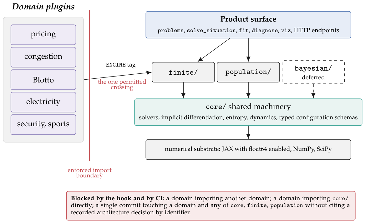
Figure 2.
The plugin contract: five declared objects plus an engine tag, and the branch taken when no conjugate field can be named.
Figure 2.
The plugin contract: five declared objects plus an engine tag, and the branch taken when no conjugate field can be named.
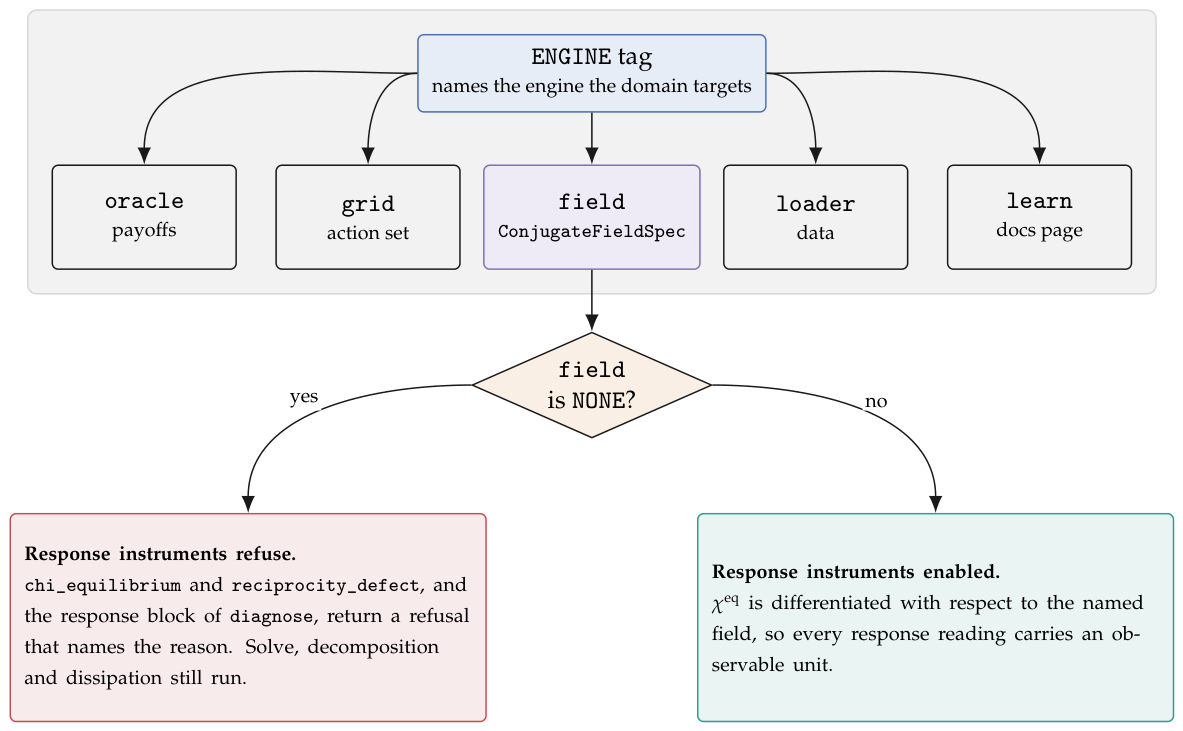
Figure 3.
The single factorisation of and the three readings it serves.
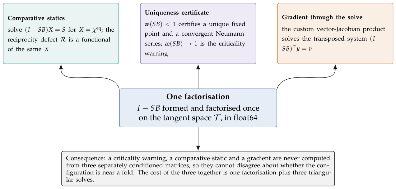
Figure 4.
Measured value against declared requirement for every row of Table 5 and Table 6 that has both as a number. Points below the diagonal pass and the vertical distance below it is the margin. Rows whose measured value is exactly zero cannot appear on a logarithmic axis and are absent: the Beckmann gradient, the symmetry defect and the spectral reality check.
Figure 4.
Measured value against declared requirement for every row of Table 5 and Table 6 that has both as a number. Points below the diagonal pass and the vertical distance below it is the margin. Rows whose measured value is exactly zero cannot appear on a logarithmic axis and are absent: the Beckmann gradient, the symmetry defect and the spectral reality check.
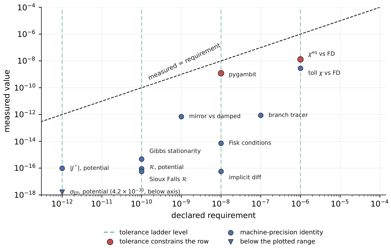
Figure 5.
The evidence pipeline from committed criterion to closed unit.
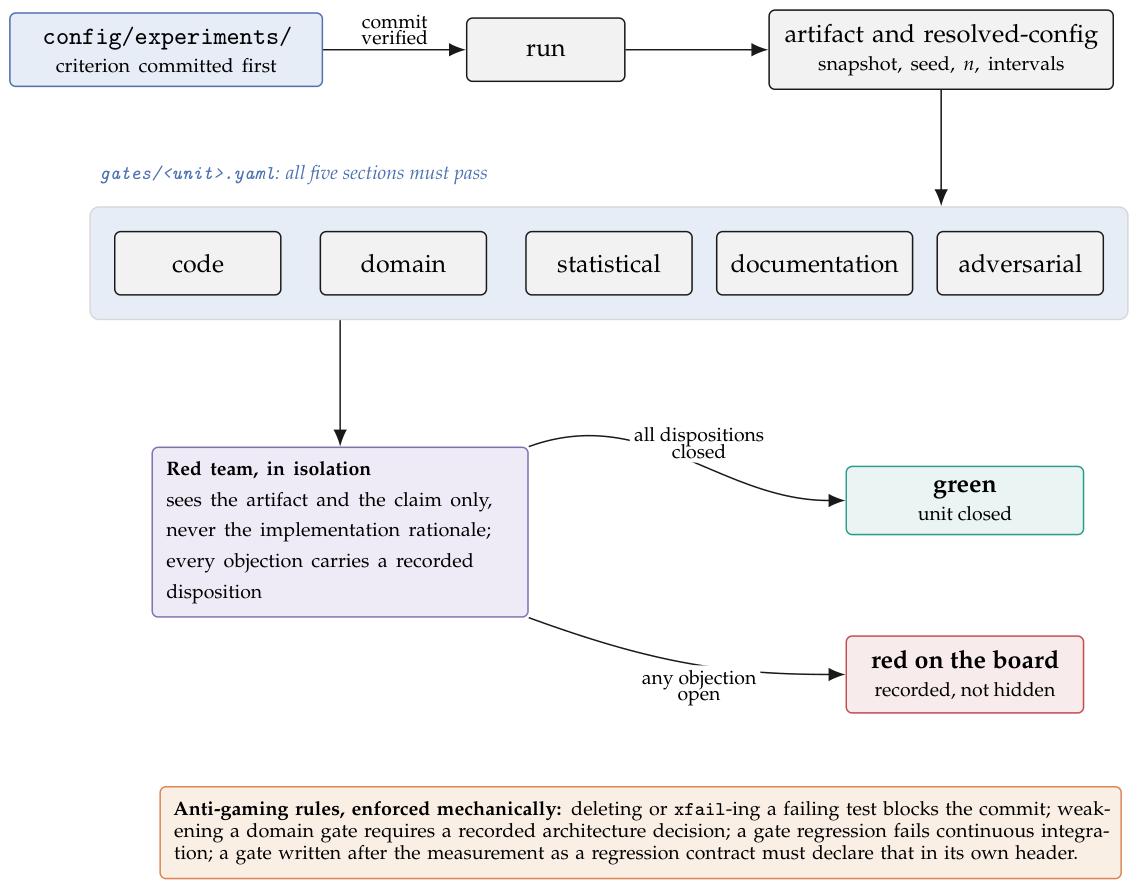
Table 1.
Capability matrix. yes means the released package exposes the capability to a user without reimplementing the method; partial is qualified in the prose below; no means it does not.
Table 1.
Capability matrix. yes means the released package exposes the capability to a user without reimplementing the method; partial is qualified in the prose below; no means it does not.
| Capability | pygambit | nashpy | OpenSpiel | QuantEcon | strataq |
|---|---|---|---|---|---|
| Logit QRE solve, strategic form | yes | no | partial | no | yes |
| Homotopy continuation in | yes | no | no | no | yes |
| Extensive-form agent QRE | yes | no | no | no | yes |
| Equilibrium derivative | no | no | no | no | yes |
| Candogan decomposition and | no | no | no | no | yes |
| Entropy production of the revision chain | no | no | no | partial | yes |
| Trajectory dissipation estimators | no | no | no | no | yes |
| Panel-aware precision estimation with intervals | partial | no | no | no | yes |
| Install with no compiler on every platform | partial | yes | partial | yes | yes |
Table 2.
Notation used throughout.
| Symbol | Meaning |
|---|---|
| N, i | number of players, player index |
| , a | number of actions of player i, an action index |
| , | mixed strategy of player i, the profile |
| payoff to player i at pure profile a | |
| , | precision of player i, common precision when uniform |
| normalised precision, times the payoff range | |
| logit response curvature, | |
| S | block susceptibility, |
| B | externality matrix, |
| tangent space | |
| Helmert basis of the tangent space of player i | |
| partial susceptibility, opponents held fixed | |
| equilibrium susceptibility, the strategic resolvent | |
| reciprocity defect, the normalised asymmetry of | |
| harmonic fraction of the normalised game | |
| spectral radius of on | |
| exact potential of a potential game | |
| , | stationary law and stationary currents of the revision chain |
| Schnakenberg entropy production rate of the revision chain | |
| , | housekeeping and excess parts of |
| , P | uniformisation rate and skeleton chain |
| k | block order of the trajectory Kullback–Leibler estimator |
| a time-integrated current over a window of horizon T |
Table 3.
Modules, principal callables, engine and gate unit. A dash in the gate column means the module has tests but no gate record.
Table 3.
Modules, principal callables, engine and gate unit. A dash in the gate column means the module has tests but no gate record.
| Module | Principal callables | Engine | Gate unit |
|---|---|---|---|
| core.solve | logit_qre, mirror, homotopy, implicit | all | solve.advanced, solve.branch |
| finite.response | chi_partial, chi_equilibrium, reciprocity_defect, strategic_spectrum, critical_lambda | finite | finite.response.reciprocity |
| finite.decompose | hodge_decompose, alpha, make_family | finite | finite.response.reciprocity |
| core.dynamics | Glauber generator, stationary law, currents , exact , uniformised sampler | finite | dynamics.exact |
| thermo.estimators | k-block KLD estimator, tur_epr_bound_ci | finite | thermo.estimators |
| thermo.nulls | reversibilised-Markov null, phase-randomised and amplitude-adjusted surrogates | finite | – |
| thermo.protocols | Hatano–Sasa split, stepwise -quench protocols, fluctuation-theorem checks | finite | thermo.protocols |
| thermo.hs_estimator | plug-in quench estimator, relaxation_gate | finite | thermo.hs_estimator |
| estimate.lam | four estimators, agreement protocol | finite | estimate.lambda |
| estimate.bayes | grid posterior with resolution guard, mixture Bayes factors, experiment selection | finite | estimate.bayes |
| population | Fisk stochastic user equilibrium, Beckmann potential, symmetry, toll susceptibility | population | population.core |
| problems | PricingProblem, AuctionProblem, RoutingProblem, AllocationProblem, ElectricityProblem | both | – |
| toolkit | diagnose, solve_situation, fit | finite | product.toolkit |
| repeated | Moore-machine strategies, folk-theorem queries, Edgeworth cycle measurement | finite | – |
| evolutionary | replicator dynamics, logit dynamic, Moran process, compare_intensity | finite | – |
| extensive | tree constructors, reduced normal form, backward induction, agent QRE | finite | – |
| viz | shared palette and plotting helpers | – | – |
| api | HTTP endpoints for the five problem types | – | api.core |
Table 4.
The tolerance ladder. Level is the declared requirement a comparison of that kind must meet.
Table 4.
The tolerance ladder. Level is the declared requirement a comparison of that kind must meet.
| Level | Kind of comparison | What sets it |
|---|---|---|
| exact analytic identities | closed-form identities that should hold to rounding; the level is a floor against catastrophic cancellation, not a calibrated threshold | |
| decomposition and solver convergence | accumulation over the projection, the decomposition and the fixed-point iteration | |
| cross-checks against an external implementation | the other implementation’s own convergence criterion is not controlled here, so the level is set by what an external oracle can be asked to guarantee | |
| finite-difference comparisons | truncation of the difference quotient at the step size used, which dominates every other error in the comparison |
Table 7.
The four rows decided by something outside this project.
| What decides | What it decides | Sample | Result | Evidence status |
|---|---|---|---|---|
| pygambit logit homotopy (Savani and Turocy, 2026; Turocy, 2005) | the fixed-precision profile is the equilibrium | 32 seeded games, 2 precisions | committed artifact gambit_agreement | |
| pygambit extensive-form logit solver | the agent QRE at every information set | 4 classic trees | inside | test suite only, skippable, no committed artifact |
| Central finite differences | is the derivative of the equilibrium | 50 random games | committed artifact chi_fd_agreement | |
| Fisk’s theorem (Fisk, 1980) and the Beckmann potential | the population engine sits at the stochastic user equilibrium | Braess diamond and Sioux Falls | 0 and | committed artifact population_identities, sioux_falls_calibration |
Table 8.
Three facts about the finite-time bound, each of which changed the reported number and each of which is now a regression test.
Table 8.
Three facts about the finite-time bound, each of which changed the reported number and each of which is now a regression test.
| Fact | Mechanism | Effect on the number | Status |
|---|---|---|---|
| The bound is a fixed-horizon statement | fixing the jump count in place of the horizon removes the Poisson fluctuation in the number of transitions, which is part of | the quantity called a bound exceeded the true rate by about | fixed-horizon windows are mandatory and are asserted |
| Two finite-sample biases | at M windows the sample version carries a term in the numerator, and Jensen’s inequality applied to biases the ratio upward | both inflate the bound towards and past the truth | both corrections applied and tested |
| The debiased point estimate legitimately straddles the truth | near equilibrium the relation saturates, so the sampling distribution of the point estimate is centred at the truth and half of it lies above | the point estimate exceeded the exact rate at 2 of 10 sweep levels, maximum ratio | the certified statement is the lower bootstrap quantile, which stayed below the exact rate at every level |
Table 9.
Failure modes at the boundary between the repository and the released package.
| Mode | Mechanism | Diagnostic | Mitigation |
|---|---|---|---|
| Packaging boundary | a data file the code loads at run time is present in the working tree and absent from the built distribution, so every in-repository test passes and the installed package fails | out-of-tree smoke test that imports the installed wheel and exercises a solver path, not only a dependency-free path | four release-integrity tests plus a continuous-integration wheel smoke on a solver path; standing rule that no release ships without an out-of-tree smoke of every public entry point |
| Version literal drift | __version__ maintained as a hand-edited literal diverges from the version in the project metadata, so a bug report names a version that never existed | equality assertion between the runtime attribute and the packaged metadata | release-integrity test asserting the equality, run before upload |
| Skippable oracle | an external comparison guarded by an optional dependency is skipped when that dependency is absent, and the suite reports a pass indistinguishable from one in which the comparison ran | presence of a committed artifact for the comparison, which a skip cannot produce | promotion of the comparison to a committed benchmark artifact; named, not yet done for the extensive-form oracle (Section 8) |
| Empty golden directory | the reference values against which drift would be detected are regenerated by the same code whose drift is in question, so a systematic change moves reference and measurement together | version-controlled difference on a regenerated artifact, which exposes any change in a committed number | artifacts are committed, so the difference is the drift check in place today; frozen cross-version golden files are named, not yet done |
Table 10.
Dependencies, their role and the version the readings of this paper were produced against. Not extracted means the resolved version is recorded in each artifact’s environment record and was not carried into this manuscript.
Table 10.
Dependencies, their role and the version the readings of this paper were produced against. Not extracted means the resolved version is recorded in each artifact’s environment record and was not carried into this manuscript.
| Package | Role | Status | Version tested |
|---|---|---|---|
| JAX (Bradbury et al., 2018) | array programming, automatic differentiation, just-in-time compilation, 64-bit arithmetic | required | not extracted |
| NumPy (Harris et al., 2020) | array interchange and the dependency-free numerical helpers | required | not extracted |
| SciPy (Virtanen et al., 2020) | sparse and dense linear algebra, optimisation and statistical routines | required | not extracted |
| Matplotlib (Hunter, 2007) | the shared palette and every plot | extra viz | not extracted |
| pygambit (Savani and Turocy, 2026) | external oracle for the solver comparisons of Section 8 | optional, test time only | 16.7.0 |
| Python | language runtime | required | 3.11 |
Disclaimer/Publisher’s Note: The statements, opinions and data contained in all publications are solely those of the individual author(s) and contributor(s) and not of MDPI and/or the editor(s). MDPI and/or the editor(s) disclaim responsibility for any injury to people or property resulting from any ideas, methods, instructions or products referred to in the content. |
© 2026 by the authors. Licensee MDPI, Basel, Switzerland. This article is an open access article distributed under the terms and conditions of the Creative Commons Attribution (CC BY) license (http://creativecommons.org/licenses/by/4.0/).
Copyright: This open access article is published under a Creative Commons CC BY 4.0 license, which permit the free download, distribution, and reuse, provided that the author and preprint are cited in any reuse.