

Submitted:
07 October 2026
Posted:
09 October 2026
You are already at the latest version
Abstract
Let \(G\) be an \(r\)-regular graph of order \(n\), \(r \ge 1\), and form \(G^{(\mathbf{m})}\) by attaching \(m_v\) pendants to each core vertex \(v\). For a symmetric degree-based weight \(\varphi\), define \[ I_\varphi(H) = \sum_{uv \in E(H)} \varphi(d_H(u), d_H(v)). \] For reassignments of a fixed thorn multiset among core vertices, a multilevel decomposition expresses all placement dependence as a weighted sum of cuts between core-degree classes. The cut between classes \(a\) and \(b\) has coefficient \(-\tfrac12 \Delta\varphi(a,b)\), where \(\Delta\varphi(a,b) = \varphi(a,a) - 2\varphi(a,b) + \varphi(b,b)\). For a fixed core and a finite nonempty set \(A\) of attainable degrees, every thorn multiset whose core-vertex degrees lie in \(A\) is reassignment-invariant if and only if \(G\) is complete or the restriction of \(\varphi\) to \(A \times A\) is a symmetric sum matrix. Requiring invariance for every connected \(r\)-regular core with \(r \ge 2\) leaves only the sum-matrix case. With two thorn levels, \(I_\varphi\) is affine in the induced-edge count \(e_G(S)\) of the \(k\) vertices receiving the larger thorn number. This determines the complete value set, exact range, and fixed-cardinality invariance criterion. On cubic cores, minimizing the index is NP-hard when the affine coefficient is positive, and maximizing it is NP-hard when the coefficient is negative. For fixed \(k\), the mean and variance of \(e_G(S)\) under uniform \(k\)-set sampling depend only on \(n\) and \(r\). For \(3 \le k \le n-3\), the third factorial moment determines the triangle count, as does the index distribution when the affine coefficient is nonzero. Cycles and equal-part complete multipartite cores admit exact ranges, with consequences for Sombor-type indices. The results connect degree-based edge indices with quadratic assignment, fixed-cardinality induced-subgraph optimization, and random induced-subgraph statistics.
Keywords:
thorny graph
; degree-based edge index
; induced-edge count
; quadratic assignment
; sum matrix
; random induced subgraph
; Sombor index
MSC: 05C09; 05C35; 05C92; 68Q25
1. Introduction
Let G be a finite simple graph with vertices , and let be non-negative integers. The thorny graph of G is obtained by attaching pendant vertices to for every i. This construction was introduced by Gutman [1]. When , the resulting graph is called thorn-regular [2].
A broad class of vertex-degree-based (VDB) indices can be written as
where is a fixed symmetric function. This is the VDB representation in terms of edge counts between prescribed degree classes [3], and it includes the Sombor index and many of its variants.
Fix a regular core and a multiset of thorn numbers, and permute the thorn numbers among the core vertices. The resulting core-edge weights may vary with the assignment. The questions concern exact criteria for reassignment invariance, the attainable values and range, and the complexity of finding an extremal placement.
The pendant-edge contribution depends only on the thorn multiset, so all variation lies in the core-edge term, a quadratic assignment objective. If the interaction matrix is a sum matrix, this objective is constant on a regular core by the sum-matrix property [4], while additive degree-based edge weights reduce to vertex sums [5]. These facts give sufficient conditions for invariance but do not determine the residual dependence for a general symmetric weight.
For comparison, Gutman [2] obtained a general formula for the ordinary Sombor index of thorny graphs. Its specialization to a uniform thorn number on a regular core appears in [2]. Here the attachment counts need not be uniform, and their assignment to the core vertices is part of the problem.
For any finite number of thorn levels, the placement-dependent term is a weighted sum of cuts. The cut between degree classes a and b has coefficient , where
The decomposition also gives an exact invariance characterization. For a fixed r-regular core with and a finite nonempty set of admissible core-vertex degrees, every thorn multiset whose core-vertex degrees lie in that set is reassignment-invariant precisely when the core is complete or the restricted weight matrix is a symmetric sum matrix. Requiring invariance over every connected r-regular core with removes the complete-graph exception.
With two thorn levels, let S be the k vertices carrying the larger thorn number. The index is affine in , so fixed-cardinality induced-edge counts govern its value set, range, and extrema. Apollonio [6] attributes the fixed-order characterization for ordinary graphs to earlier papers by Akiyama, Exoo and Harary, by Bosák, and by Širáň. The fixed-core criterion below uses Caro’s formulation [7]. The same affine relation shows that minimizing the index is NP-hard on cubic cores when the two-level coefficient is positive, while maximizing it is NP-hard when the coefficient is negative. For a regular core and fixed k, Apollonio’s formulas for the first two binomial moments of the induced-edge count [6] reduce to expressions involving only the order and regular degree of the core. For , the third factorial moment determines the number of triangles. Thus regular cores with the same order and degree have the same mean and variance for under uniform k-set sampling, although their distributions may differ. The two-level reduction therefore connects thorn reassignment with fixed-cardinality induced-subgraph optimization, computational complexity, and random induced-subgraph statistics.
2. Preliminaries
All graphs are finite, simple, and undirected. Let G be an r-regular graph of order n, where . For a vector of non-negative integers, write for the thorny graph obtained by attaching pendant vertices to v.
The degree of a core vertex v in is
while every new pendant vertex has degree 1. For a fixed symmetric weight , the index splits as
Write
This term depends only on the multiset of the values .
Let
where the are distinct. Put
For disjoint vertex sets , let be the number of edges with one endpoint in X and the other in Y. Write for the number of edges induced by X.
For positive integers , define
This quantity is the second difference of at a and b. Çela, Deineko and Woeginger [4] define a sum matrix by . For symmetric matrices, this definition is equivalent to the following condition.
Lemma 1.
Let . The restriction of φ to is a symmetric sum matrix if and only if for all .
Proof.
If , then for all . Conversely, if all these second differences vanish, set . Then
for all . □
The residual coefficient for the cut between the classes and is .
A reassignment of a thorn multiset means replacing by a vector obtained by permuting its entries among the vertices of the same core G. The sets and the multiplicities remain fixed, but the vertex classes may change.
3. Main Results
3.1. The Cut Decomposition
For degree-based edge-weight indices, an additive edge weight reduces to a vertex sum [5]. The following identity separates the additive part from the residual cut term.
Theorem 1.
Let G be an r-regular graph, let be a thorn vector, and use the notation above. Then
In particular, for a fixed thorn multiset, all placement dependence is contained in the final weighted cut sum.
Proof.
For a core edge with and , write
When , the last term is zero. Summing the first two terms over the core edges counts once for every core edge incident with v. Since G is r-regular, their total is
Corollary 1.
Let and be reassignments of the same thorn multiset on G. Let and be the classes of core vertices having degree in and , respectively. Then
Proof.
The pendant term and the diagonal term in Theorem 1 depend only on the multiset and therefore cancel. □
The next characterization does not require the core to be connected. The sum-matrix implication follows from [4], while the necessity can also be deduced from the characterization of linearizable symmetric Koopmans–Beckmann quadratic assignment problems due to Punnen and Kabadi [8]. The proof below gives a direct argument in terms of the second difference.
Theorem 2.
Let G be an r-regular graph of order n, where , and let be finite and nonempty. The following are equivalent.
- (i)
- Any two reassignments of any thorn multiset for which all core vertices have degrees in A in the resulting thorny graph have the same -value on G.
- (ii)
- The graph G is complete, or the restriction of φ to is a symmetric sum matrix.
Proof.
If the restriction is a sum matrix, Lemma 1 and Theorem 1 give invariance. If G is complete, the core-edge sum runs over all unordered pairs of core vertices and therefore depends only on the multiset of assigned degrees. The pendant term has the same property.
Conversely, suppose that G is not complete and that (i) holds. If , the restriction is a sum matrix. Assume therefore that . Since , the graph has an edge . Because it is not complete, it also has a non-edge . Fix distinct . Attach thorns to x and y and thorns to every other vertex. Compare this placement with the one that attaches thorns to u and v and thorns to every other vertex. For a two-vertex b-class S, regularity gives
The two cut sizes differ by 2, because and . Corollary 1 therefore gives the index value for the placement at minus that for the placement at as . Condition (i) implies . Since were arbitrary, Lemma 1 proves that the restriction is a sum matrix. □
The complete-graph exception is essential. Every symmetric edge weight gives a reassignment-invariant index there because every pair of core vertices is adjacent. For invariance over all connected regular cores, that exception disappears as soon as .
Corollary 2.
Fix an integer and a finite nonempty set . The following are equivalent.
- (i)
- The restriction of φ to is a symmetric sum matrix.
- (ii)
- For every connected r-regular graph G and every thorn multiset for which all core vertices have degrees in A in the resulting thorny graph, all reassignments of that multiset have the same -value.
Proof.
The implication (i)⇒(ii) follows from Theorem 1. Conversely, apply (ii) to the connected non-complete r-regular graph and invoke Theorem 2. □
3.2. Two Thorn Levels and Induced Subgraphs
Fix as the two possible thorn numbers. Put
Let be the set of k vertices receiving q thorns. Every vertex outside S receives p thorns. Denote the resulting thorny graph by .
Theorem 3.
With the notation above,
Consequently, for two k-subsets ,
Proof.
The number of core edges with both endpoints in S is . Since the sum of the degrees in G of the vertices in S is , the number of core edges with exactly one endpoint in S is . The remaining core edges have both endpoints outside S. Hence the core contribution is
which simplifies to the first three terms in (4). The final two terms are the pendant contribution. Subtracting the formulas for S and T gives (5). □
For , define
Then
Corollary 3.
Let G be an r-regular graph of order n. Fix and , and put and . Set
Let be the set of all values with and . Then
The value-set identity has the following consequences.
- If , all placements have the same value.
- If , two placements have the same value if and only if their selected k-sets induce the same number of edges.
- The range of the index over all placements is
If , the maximum occurs on the densest selected k-sets and the minimum on the sparsest ones. If , the directions are reversed.
Proof.
The value-set identity is the affine formula in Theorem 3 with ranging over . The remaining assertions follow from the same identity. □
Caro’s fixed-order characterization [7] is stated below.
Lemma 2.
Let H be a graph of order n, and fix k with . If has the same value for every k-subset , then H is complete or edgeless.
Applying this characterization to Theorem 3 gives the following placement criterion.
Corollary 4.
Let G be an r-regular graph of order n, let , and let vertices receive q thorns. All placements have the same -value if and only if at least one of the following holds.
- .
- .
- G is complete.
In particular, if G is not complete, , and , then at least two placements have different values.
Proof.
The three stated conditions are sufficient. The first follows from Theorem 3. For or there is only one placement. For , every selected set induces no edge. For , the selected set induces edges. On a complete graph, every k-set induces edges.
Conversely, suppose none of the three conditions holds. Then , the second difference is nonzero, and G is neither complete nor edgeless. Lemma 2 gives two k-sets with different induced-edge counts. Equation (5) shows that the corresponding index values are different. □
Proposition 1.
Let G be r-regular of order n and size . For ,
In particular,
Proof.
For every k-set S, regularity gives
Taking maxima and minima proves the result. □
3.2.1. Computational Complexity
Minimizing over all k-subsets is the k-sparsest subgraph problem, a fixed-cardinality graph-partitioning problem [9]. Fomin et al. studied fixed-parameter approximation within the fixed-cardinality graph-partitioning family [10]. For a nonzero two-level coefficient, Theorem 3 shows that minimizing the index when the coefficient is positive, or maximizing it when the coefficient is negative, is equivalent to minimizing . Maximum Independent Set is APX-complete even on 3-regular Hamiltonian graphs [11].
Theorem 4.
Fix two integers and a symmetric weight φ such that
Given a 3-regular graph G and an integer k with , finding a k-subset that minimizes when the second difference is positive, or maximizes it when the second difference is negative, is NP-hard. Here , and φ are fixed and are not part of the instance.
Proof.
Put and . By Theorem 3, there is a quantity , independent of S, such that
The graph G has an independent set of size at least k if and only if it has a k-set S with . If the second difference is positive, a minimizing placement has value C exactly when such an independent set exists. If the second difference is negative, the same statement holds for a maximizing placement. Consequently, a polynomial-time algorithm for the placement problem on 3-regular Hamiltonian cores would decide Independent Set on the same class in polynomial time. The claimed NP-hardness follows. □
The reduction proves hardness only when solving the index problem amounts to minimizing . It gives no conclusion when solving it amounts to maximizing .
Remark 1.
The distinction between a fixed core and all regular cores is essential. On the complete graph , every k-set induces edges, so every symmetric weight gives the same index value for all placements of any two-level thorn multiset. Corollary 2 concerns invariance over all connected r-regular cores, where a nonzero second difference is exposed by .
Remark 2.
Every automorphism orbit on the k-subsets of is contained in a single index-value class. When the two-level second difference is nonzero, the converse need not hold. The index depends only on the number of edges induced by the selected k-set, not on its full orbit or isomorphism type.
3.2.2. Random Placements and Induced-Edge Moments
Choose S uniformly from the k-subsets of and put . Alon, Hefetz, Krivelevich and Tyomkyn [12] studied fixed-order induced subgraphs with prescribed edge counts. At discrete time k, the edge count in Janson’s random vertex-uncovering process has the same distribution as [13]. Apollonio [6] computed the first two binomial moments of for arbitrary graphs. For regular cores, these moments yield the following mean and variance formulas.
For a non-negative integer x, write and for . For , put
Lemma 3.
Let G be an r-regular graph of order , and choose S uniformly from the k-subsets of , where . Put
and let . Then
Proof.
For a core edge e, let indicate that both endpoints lie in S. Then gives . Of the unordered pairs of core edges, Q share a vertex and R are disjoint. Thus , and the variance identity gives the second formula. □
For fixed k, the displayed formulas depend on the core only through n and r. Since the index is affine in X, its mean and variance follow from the same formulas.
Corollary 5.
Retain the notation of Lemma 3. Fix , put and , and let C denote the part of (4) independent of S. Then
Proof.
Apply the affine identity . □
Theorem 5.
Assume . Let be the number of triangles of G, and retain the notation of Lemma 3. Define
Then
Consequently, if , the distribution of X determines . Under the same condition on k, for any fixed with , the distribution of the corresponding two-level index values determines as well.
Proof.
Expand over ordered triples of distinct core edges. For an unordered triple of edges, the probability that all three belong to the induced subgraph on S is when their union has j vertices. There are triples whose union is a triangle. The triples with four vertices consist of three-edge stars and three-edge paths. Their number is
A three-edge path is determined by its middle edge and one incident edge chosen at each endpoint, giving choices. Each triangle gives three choices whose selected edges form the triangle rather than a path, so these choices must be excluded.
A triple with five vertices has one adjacent pair of selected edges and a third edge disjoint from their three vertices. For an adjacent pair whose outer vertices are not adjacent, the number of eligible third edges is . If the outer vertices are adjacent, the pair lies in a triangle and the number is . Since the adjacent pairs include exactly pairs of the second type, the total is
The remaining triples are matchings of size three. Hence
The coefficient of simplifies to
which proves (10). This coefficient is positive for . For fixed with , the affine relation in Theorem 3 recovers X from the index value. □
Remark 3.
Unlike the mean and variance, the full distribution need not be determined by n and r. For , the event means that S spans a triangle. The triangular prism has two such triples, whereas has none. Thus these two cubic graphs of order six have the same mean and variance in Lemma 3, but different placement distributions whenever the two-level second difference is nonzero.
3.3. Exact Ranges for Two Core Families
Corollary 3 reduces the range problem to computing and .
3.3.1. Cycle Cores
Vasilev [14] proved that consecutive vertices maximize the number of induced edges in every power of a cycle. The next proposition specializes this result to an ordinary cycle and also determines the minimum. A direct proof is included.
Proposition 2.
Let , where , and let . Then
Consequently, for fixed , the range of the two-level index on is
Proof.
A set of consecutive vertices induces a path with edges, and no induced subgraph on k vertices of a cycle can contain more edges. This proves the maximum.
For a nonempty proper subset S of a cycle, let be the number of runs of consecutive selected vertices. Then . The number of runs is at most k and at most , because distinct runs require distinct unselected gaps. The bound is sharp, so
Therefore . The range formula follows from Corollary 3. □
For fixed and , the index value for an adjacent placement minus that for a non-adjacent placement is . These two placements are used again in SubSection 3.4.
3.3.2. Equal-Part Complete Multipartite Cores
Proposition 3.
Let be the complete t-partite graph with parts of size . Thus and G is -regular. For , write
and
Then
Consequently, for fixed , the exact two-level placement range is times the difference between (11) and ().
Proof.
Let be the number of selected vertices in the ith part. Then , , and
The last sum is minimized when the differ by at most one, which gives u entries equal to and equal to ℓ. It is maximized by filling parts successively, which gives c entries equal to s, one entry equal to d when , and all remaining entries zero. These are exactly (11) and (). □
Corollary 6.
For and ,
Proof.
Apply Proposition 3 with and . Balancing the selected vertices between the two parts gives . Concentrating them in one part as far as possible gives for and for . □
3.4. Consequences for Sombor-Type Indices
Consider the following five degree-based weights. The ordinary and reduced Sombor weights are
The ordinary and reduced Sombor indices were introduced by Gutman [15]. The elliptic and Euler Sombor weights are, respectively,
The elliptic Sombor index was introduced in [16]. The Euler Sombor weight displayed above is the one defined in [17]. The forgotten index, revisited by Furtula and Gutman [18], has edge weight .
For with , direct calculation gives
The first three inequalities follow from , with replaced by for the reduced weight. For the Euler weight,
Thus, for each fixed pair , Theorem 4 shows that, on cubic cores, it is NP-hard to minimize the elliptic Sombor index and to maximize any of the ordinary, reduced, and Euler Sombor indices.
Corollary 7.
Fix an r-regular core G of order n, two thorn numbers , and the number of vertices receiving q thorns.
- The ordinary Sombor, reduced Sombor, and Euler Sombor indices are maximized when the selected k-set induces as few core edges as possible and minimized when it induces as many as possible.
- The elliptic Sombor index is maximized on the densest selected k-sets and minimized on the sparsest ones.
- The forgotten index is independent of the placement.
For each non-additive weight, the exact range is the absolute value of the corresponding expression in (13)–() multiplied by .
Proof.
Apply Corollary 3 and the signs above. □
Example 1.
Let the core be . For a two-set S, attach two pendants at each vertex of S and one at each vertex outside S. Thus , , and . If S is an edge, then . If the two vertices of S are antipodal, then . The adjacent value minus the antipodal value is . Table 1 gives the resulting values.
Figure 1 illustrates the two placements. Their exact comparison follows from Theorem 3.
3.5. Relation to the Uniform Case
If for every v, write . All core vertices have the same degree in . The cut sum in Theorem 1 is empty, and
Equation (18) is the VDB degree-pair evaluation of the uniform construction [3]. For the ordinary Sombor weight, formula (18) coincides with the regular thorn-regular formula in [2].
Thus (18) serves only to connect the present formulas with the uniform case. The results for non-uniform attachments include the cut decomposition, the fixed-core and universal invariance criteria, the two-level ranges, the third-factorial-moment formula, and the complexity result.
4. Conclusions
For a fixed thorn multiset on a regular core, reassignment leaves the pendant-edge contribution unchanged and concentrates all remaining placement dependence in a weighted cut sum. This gives the fixed-core characterization. For an r-regular core with and a finite nonempty degree set A, every thorn multiset with core-vertex degrees in A is reassignment-invariant precisely when the core is complete or the restriction of to is a symmetric sum matrix. Requiring the same invariance for every connected r-regular core with leaves only the sum-matrix alternative.
With two thorn levels, the placement problem reduces to . This reduction determines the complete value set, exact range, and fixed-cardinality invariance criterion. For a nonzero affine coefficient, the extremal-placement problem is a fixed-cardinality induced-subgraph optimization problem. On cubic cores, minimizing the index is NP-hard for a positive coefficient, while maximizing it is NP-hard for a negative coefficient. For fixed k, the mean and variance of under uniform k-set sampling depend on the core only through n and r. For , the third factorial moment determines the triangle count. Exact ranges for cycles and equal-part complete multipartite cores, together with the Sombor-type consequences, illustrate the same reduction.
Regularity underlies this separation. On a non-regular core, the diagonal term can itself depend on the thorn assignment, so the original degree sequence interacts with the thorn levels. Such cores are not covered by the present characterization.
Conflicts of Interest
The author declares no known competing financial interests or personal relationships that could have appeared to influence the work reported in this paper.
References
- Gutman, I. Distance of thorny graphs. Publ. Inst. Math. (Beograd) 1998, 63(77), 31–36. [Google Scholar] [CrossRef]
- Gutman, I. Sombor index of thorny graphs. Vojnoteh. Glas. 2025, 73(2), 413–422. [Google Scholar] [CrossRef]
- Rada, J.; Cruz, R. Vertex-degree-based topological indices over graphs. MATCH Commun. Math. Comput. Chem. 2014, 72, 603–616. [Google Scholar]
- Çela, E.; Deineko, V.G.; Woeginger, G.J. Well-solvable cases of the QAP with block-structured matrices. Discret. Appl. Math. 2015, 186, 56–65. [Google Scholar] [CrossRef]
- Hu, Z.; Li, L.; Li, X.; Peng, D. Extremal graphs for topological index defined by a degree-based edge-weight function. MATCH Commun. Math. Comput. Chem. 2022, 88, 505–520. [Google Scholar] [CrossRef]
- Apollonio, N. Second-order moments of the size of randomly induced subgraphs of given order. Discret. Appl. Math. 2024, 355, 46–56. [Google Scholar] [CrossRef]
- Caro, Y. On graphs with prescribed subgraphs of order k, and a theorem of Kelly and Merriell. Czechoslov. Math. J. 1994, 44, 623–629. [Google Scholar] [CrossRef]
- Punnen, A.P.; Kabadi, S.N. A linear time algorithm for the Koopmans–Beckmann QAP linearization and related problems. Discret. Optim. 2013, 10(3), 200–209. [Google Scholar] [CrossRef]
- Shachnai, H.; Zehavi, M. Parameterized algorithms for graph partitioning problems. Theory Comput. Syst. 2017, 61, 721–738. [Google Scholar] [CrossRef]
- Fomin, F.V.; Golovach, P.A.; Inamdar, T.; Koana, T. FPT approximation and subexponential algorithms for covering few or many edges. Inf. Process. Lett. 2024, 185, 106471. [Google Scholar] [CrossRef]
- Lozin, V.V.; Monnot, J.; Ries, B. On the maximum independent set problem in subclasses of subcubic graphs. J. Discret. Algorithms 2015, 31, 104–112. [Google Scholar] [CrossRef]
- Alon, N.; Hefetz, D.; Krivelevich, M.; Tyomkyn, M. Edge-statistics on large graphs. Comb. Probab. Comput. 2020, 29, 163–189. [Google Scholar] [CrossRef]
- Janson, S. Uncovering a graph. Probab. Theory Relat. Fields 2026, 195, 689–740. [Google Scholar] [CrossRef]
- Vasilev, K. The edge-isoperimetric inequality for powers of cycles. Math. Educ. Math. 2026, 55, 78–84. [Google Scholar] [CrossRef]
- Gutman, I. Geometric approach to degree-based topological indices: Sombor indices. MATCH Commun. Math. Comput. Chem. 2021, 86, 11–16. [Google Scholar]
- Gutman, I.; Furtula, B.; Öz, M.S. Geometric approach to vertex-degree-based topological indices: elliptic Sombor index, theory and application. Int. J. Quantum Chem. 2024, 124(2), e27346. [Google Scholar] [CrossRef]
- Gutman, I. Relating Sombor and Euler indices. Vojnoteh. Glas. 2024, 72(1), 1–12. [Google Scholar] [CrossRef]
- Furtula, B.; Gutman, I. A forgotten topological index. J. Math. Chem. 2015, 53, 1184–1190. [Google Scholar] [CrossRef]
Figure 1.
Two placements of the thorn multiset on the cycle core . The black core vertices form S and receive two pendants, while each core vertex outside S receives one pendant. In (a), the vertices of S are adjacent and , whereas in (b) they are antipodal and .
Figure 1.
Two placements of the thorn multiset on the cycle core . The black core vertices form S and receive two pendants, while each core vertex outside S receives one pendant. In (a), the vertices of S are adjacent and , whereas in (b) they are antipodal and .
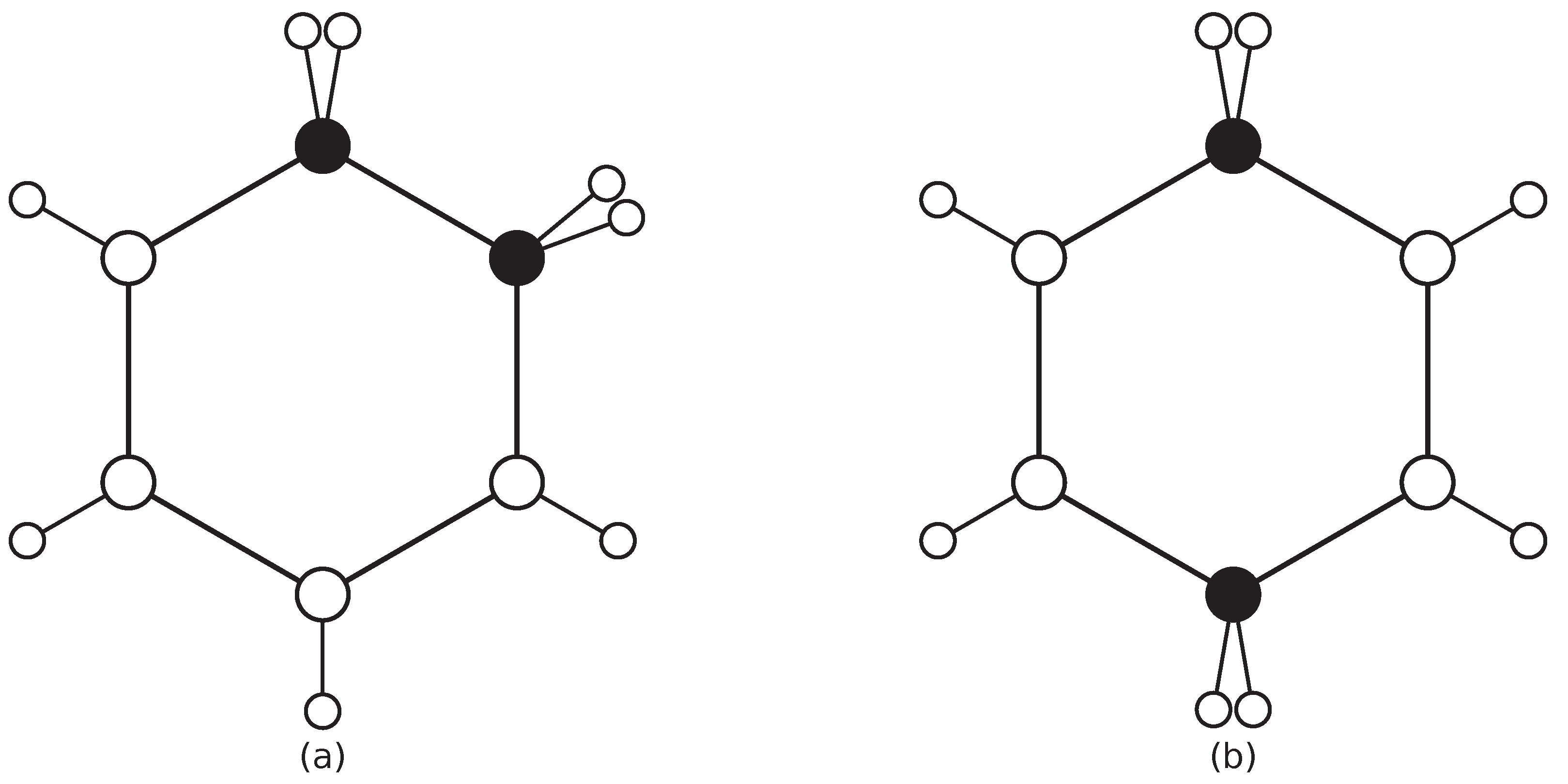

Table 1.
Two placements of the thorn multiset on .
| Index | Adjacent | Antipodal | Adjacent minus antipodal |
|---|---|---|---|
| SO | |||
| ESO | |||
| EU | |||
| Forgotten F | 244 | 244 | 0 |
Disclaimer/Publisher’s Note: The statements, opinions and data contained in all publications are solely those of the individual author(s) and contributor(s) and not of MDPI and/or the editor(s). MDPI and/or the editor(s) disclaim responsibility for any injury to people or property resulting from any ideas, methods, instructions or products referred to in the content. |
© 2026 by the authors. Licensee MDPI, Basel, Switzerland. This article is an open access article distributed under the terms and conditions of the Creative Commons Attribution (CC BY) license (http://creativecommons.org/licenses/by/4.0/).
Copyright: This open access article is published under a Creative Commons CC BY 4.0 license, which permit the free download, distribution, and reuse, provided that the author and preprint are cited in any reuse.