

Submitted:
19 August 2026
Posted:
21 August 2026
You are already at the latest version
Abstract
This study articulates, documents and characterizes a processed financial dataset of daily coffee, Brent oil and gold futures prices for the period 2016-2025. The database was constructed from historical closing prices obtained from Investing.com and organized in long format, so that each record corresponds to a valid daily observation of a specific commodity. Using the original series, a reproducible transformation chain was developed, including logarithmic prices, logarithmic returns, absolute returns, squared returns, 30-day annualized rolling volatility, standardized returns, base-100 price indices, temporal labels and quality-control fields. This manuscript specifically documents the dataset architecture, the information source, quotation units, data-cleaning criteria, temporal consistency and analytical reuse possibilities. The empirical characterization shows that the three markets preserve financial features such as non-Gaussian distributions, heavy tails, heterogeneous volatility and more visible dependence in additional second-moment transformations. The resource is designed to be reused in financial econometrics, econophysics, commodity risk analysis, forecasting exercises, Monte Carlo simulation, financial time-series teaching and comparative studies of agricultural, energy and precious-metal markets.
Keywords:
commodity futures
; coffee futures
; Brent oil futures
; gold futures
; financial time series
; logarithmic returns
; volatility
; long memory
; multifractality
; Monte Carlo simulation
; financial risk
1. Introduction
Commodity risk analysis, financial econometrics and data science jointly determined the importance of dataset selection in this study, because the central argument is based on the fact that coffee, Brent oil and gold futures series constitute not only market records but also empirical inputs that require curation, traceability and systematic transformation in order to be reused in analyses of volatility, temporal memory, multifractality and probabilistic scenarios.
International commodity markets concentrate information on expectations, supply restrictions, demand conditions, geopolitical tensions and changes in risk perception. Since the early formalization of speculative prices [1] and the debate on informational efficiency [2], different studies have documented irregular speculative variations [3] and stylized facts in financial returns [4], which require working with curated databases that preserve tails, extreme episodes and temporal heterogeneity. This implies that financial prices are not exhausted by linear dynamics or simple Gaussian assumptions.
Coffee was selected because it represents an agricultural market that is particularly relevant for Colombia in terms of production and exports; Brent oil represents an energy benchmark associated with external revenues, fiscal expectations and geopolitical effects; and gold represents a hedging and safe-haven commodity during episodes of uncertainty [5]. The selection of coffee, Brent oil and gold therefore responds to a comparative and strategic logic. This heterogeneity makes it possible to examine three markets with different fundamentals under a common data architecture, without eliminating the calendar, scale and behavioral differences that characterize each asset.
The financial modelling of these series is supported by derived variables capable of converting nominal prices into comparable measures of variation, intensity and risk. ARCH and GARCH statistical models implement conditional heteroscedasticity and variance persistence [6,7], while the Box-Jenkins approach makes it possible to diagnose dependence, stability and reproducible specifications [8,9]. To expand the analytical value of closing prices and facilitate economic reuse, the dataset integrates returns, magnitude measures, rolling volatility and normalized indicators [10,11].
To interpret irregular phenomena, fractal and multifractal analysis is used to recognize financial irregularity through a scaling structure [12]. Fractal market analysis proposes that the heterogeneity of investment horizons can generate dynamics that are more complex than those predicted by linear models [13]. The estimation of temporal memory originates in the analysis of persistent dependence [14] and fractional integration models [15].
Long memory establishes persistence as a phenomenon that requires careful analysis in relation to structural changes, heteroscedasticity and short-memory dependence [16,17]. The statistical analysis of long-memory processes and the use of the R/S statistic indicate the need to precisely reference the transformations applied to the series [18,19]. To study temporal scaling with explicit criteria of interpretation, robustness and reproducibility, tools such as DFA and the review of its variants are required [20,21].
When ordinary small movements and extreme events respond to differentiated scaling mechanisms, multifractality becomes relevant, and MF-DFA makes it possible to study the behavior of fluctuations of different magnitudes across temporal scales [22]. Demonstrating that financial markets exhibit regularities compatible with complex systems requires the incorporation of strong econophysics components [23]. In addition, the approach of correlations and complexity in finance broadens the perspective toward interdependent markets [24]. Moreover, to examine relationships between nonstationary series without losing their stationary structure, detrended cross-correlation analysis is required [25].
Studies have reported evidence on volatility, memory or efficiency in commodities; however, cleaning rules, metadata, derived variables and reproducibility controls have remained less visible. The FAIR data framework establishes that a scientific resource acquires value when it is findable, accessible, interoperable and reusable [26]. Data infrastructure and sharing practices show that the quality of a database depends on its organization, preservation, documentation and auditability [27,28].
In computational research, reproducibility requires inputs, transformations and analytical decisions to be verifiable by third parties [29]. When results depend on quantitative processing workflows, editorial policies on data and code reinforce the requirement for verification [30]. The use of tidy data facilitates the observational unit of each variable, consistent definition and explicit analytical function [31]. Accordingly, this article constructs a processed dataset of coffee, Brent oil and gold futures from historical records obtained from Investing.com [32].
The contribution of the study is established at three articulated levels. First, it provides a long-format database that preserves the identity of each commodity, its effective trading dates and its quotation units. Second, it documents the price-processing pipeline, from closing prices to logarithmic prices, logarithmic returns, absolute returns, squared returns, rolling volatility, base-100 indices and standardized returns. Finally, it demonstrates that the resource has the capacity to support descriptive analysis, dependence diagnostics, temporal memory, multifractality and Monte Carlo simulation. This article is organized into five sections: materials and methods, results, discussion, conclusions and final statements.
2. Materials and Methods
Describing the workflow through which historical records are transformed into a processed financial resource is a central methodological component. The procedure integrates decisions on scope, temporal control, variable construction and diagnostic validation. The objective is to enable the reader to reconstruct the path of the data from the closing price to the variables used in the tables, figures and reuse demonstrations.
2.1. Dataset
The dataset was constructed from daily closing prices of coffee, Brent oil and gold futures for the period 2016-2025. A valid daily record for a specific commodity is the observational variable. This approach preserves the sequence of each market and avoids an artificial date intersection that could alter volatility, temporal dependence or tail events.
Table 1 summarizes the financial coverage and organizes the basic information of the resource: asset type, instrument, quotation unit, source, start and end dates, and number of valid observations for prices and returns. Its purpose is to establish the empirical scope of the dataset before presenting the analytical transformations.
Table 1 shows that returns were constructed within each series without cross-sectional combination of assets. The expected loss of the first record between prices and returns is defined by the difference, because no previous price is available. This preserves temporal integrity and avoids interpolations that could introduce artificial smoothing.
2.2. Data Preprocessing and Variable Construction
To convert prices expressed in heterogeneous units into comparable financial variables, preprocessing is required. Stabilizing scale, measuring relative variations, capturing movement magnitude, approximating the second moment, documenting recent risk and normalizing trajectories are part of the precise transformation functions within the pipeline. Formalizing this process makes it possible to evaluate the database and reproduce its derived columns.
The closing price in logarithmic scale, aligned with Equation (1), is the first transformation performed. This operation preserves the temporal order of prices and facilitates the subsequent construction of continuous returns.
where represents the logarithmic price of commodity on day ; is the closing price observed for commodity i on day ; and denotes the natural logarithm operator. This variable makes it possible to work on a scale compatible with continuous returns and facilitates the comparison of series with different quotation units.
The daily logarithmic return is obtained as the continuous variation between two consecutive prices of the same commodity, according to Equation (2). The operation is executed within each asset and while respecting its own trading calendar.
where is the daily logarithmic return of commodity on day ; is the current closing price; and is the immediately preceding closing price within the same commodity. The subscript identifies the asset and the subscript identifies the trading day. This definition avoids calculating returns between different assets or unordered dates.
The absolute magnitude of movements is obtained through Equation (3). This variable removes the direction of change and preserves the intensity of the variation, making it useful for examining episodes of high market mobility.
where represents the absolute value of the logarithmic return of commodity on day ; is the daily logarithmic return; and corresponds to the absolute-value operator. This variable is useful for studying variation intensity, stress episodes and persistence in return magnitude.
The squared return, defined in Equation (4), amplifies larger variations and provides an elementary approximation to second-moment dynamics. Its inclusion makes it possible to contrast dependence in simple returns with persistence in variability.
where corresponds to the square of the logarithmic return of commodity i on day t; and represents the return raised to the square. This variable is a frequent input for diagnosing volatility dependence and risk clustering.
The 30-day annualized rolling volatility is calculated by applying Equation (5). This measure analyzes return variability and identifies stress periods without using parametric conditional models.
where represents the 30-day annualized rolling volatility of commodity on day ; 252 is the annualization factor for daily returns; is the return observed days earlier within the same commodity; is the mean return in the 30-observation rolling window; and k=0,...,29 indicates that the current return and the previous 29 valid returns are used. The measure is calculated independently for each asset.
To compare accumulated trajectories across assets with different quotation units, the base-100 index formalized in Equation (6) is used. The transformation preserves the relative dynamics of each market without artificially equating their nominal levels.
where is the normalized index of commodity on day ; is the closing price on date t; and corresponds to the first valid price in the commodity i series. This transformation does not replace return analysis, but it makes it possible to observe relative trends on a common scale.
The standardized return is defined in Equation (7). This variable centers and scales the returns of each commodity with respect to its own distribution, enabling the identification of relative extreme events within each market.
where represents the standardized return of commodity on day ; is the daily logarithmic return; is the sample mean of returns for commodity ; and is the sample standard deviation of the returns of the same asset.
2.3. Quality-Control Criteria
Quality controls ensure that the properties observed in the dataset correspond to market dynamics. Validation focuses on temporal ordering, record uniqueness, price positivity, price-return consistency, absence of interpolation and source traceability.
Table 2 identifies the field to be evaluated, the validation criterion and the relevance of each verification within the financial curation process by integrating the controls applied during construction of the resource.
Table 2 shows a reproducible audit logic applied to the dataset, in which each record preserves the asset, date, source and quotation unit; in addition, each return is calculated using information from the commodity, and derived variables are documented through explicit rules. This traceability is applied to reduce the risk of confusing processing errors with market signals.
2.4. Descriptive and Diagnostic Indicators
To evaluate whether the processed database preserves financial properties relevant for subsequent analyses, a diagnostic characterization is performed. Descriptive measures, normality, autocorrelation and joint statistics show whether the resource contains sufficient variability, tails and dependence for econometric and risk applications.
The Jarque-Bera test makes it possible to assess whether the deviation of returns follows a normal distribution. The articulation of skewness and kurtosis in Equation (8) synthesizes the distance between the empirical distribution and Gaussian behavior.
where is the Jarque-Bera statistic for commodity ; is the number of valid returns; represents sample skewness; and corresponds to Pearson kurtosis. High values of JBi are consistent with non-Gaussian distributions, a common situation in financial series with heavy tails.
The order autocorrelation in Equation (9) makes it possible to observe linear dependence in returns and second-moment dependence when applied to squared returns. This differentiates mean dynamics from variability persistence.
where is the autocorrelation of commodity at lag ; is the current return; and is the return observed periods earlier. This measure allows linear dependence to be assessed at different lags.
The Ljung-Box statistic in Equation (10) jointly evaluates the significance of autocorrelations up to lag m and summarizes temporal dependence without relying on a single isolated lag.
where represents the Ljung-Box statistic of commodity up to lag ; is the number of valid observations; is the autocorrelation of order ; and is the total number of lags evaluated. The statistic summarizes the joint significance of autocorrelations.
2.5. Reuse Demonstration: Long Memory, Multifractality and Monte Carlo
Analytical reuse is demonstrated through temporal-memory, multifractality and simulation tools. The objective is to show that the dataset variables support advanced procedures for scaling, dependence and probabilistic-scenario generation.
The R/S fraction of the Hurst coefficient is used as an initial approximation for observing temporal persistence through Equation (11). The value of this coefficient allows a preliminary analysis of scaled behavior and is interpreted together with more robust diagnostics.
where represents the cumulative range of deviations from the mean in a window of size ; s the standard deviation within that window; is a proportionality constant; and is the Hurst exponent. Values close to 0.5 are compatible with the absence of strong linear persistence.
Equation (12) presents the accumulation of data from DFA, whose transformation converts centered returns into an accumulated trajectory on which scale fluctuations are evaluated.
where represents the cumulative profile of commodity i up to temporal position ; is the logarithmic return observed at ; and is the mean return of the series. This transformation makes it possible to evaluate fluctuations around local trends.
The slope of the DFA fluctuation function defined in Equation (13), on a log-log scale, approximates scaling behavior and makes it possible to evaluate whether the series is persistent, antipersistent or close to randomness.
where represents the DFA fluctuation function of commodity for scale ; is the number of observations evaluated; is the cumulative profile; and represents the local trend estimated within each window of size s.
The generalized MF-DFA function, summarized in Equation (14), extends the analysis to different q orders, thereby making it possible to differentiate small and large fluctuations, which is relevant for markets exposed to ordinary and extreme episodes.
where represents the generalized fluctuation function of commodity for order and scale ; is the number of segments; is the local detrended variance of segment at scale . Positive values of emphasize large fluctuations and negative values emphasize small fluctuations.
By observing the trajectories described with the Monte Carlo method, probabilistic reuse becomes evident according to Equation (15). The simulation is established as a mechanism for translating the historical distribution of returns into uncertainty bands.
where is the simulated price of commodity at horizon for trajectory ; is the last observed price; is the simulated return at step of trajectory ; and is the exponential function. The equation makes it possible to construct probabilistic trajectories from simulated returns.
2.6. Computational Environment and Data Availability
Because transforming historical records into comparable financial variables, reproducing figures and auditing statistical diagnostics are necessary, the computational environment is an operational extension of the methodological design. For each commodity, the dataset is produced through a sequential workflow of chronological ordering, price-return consistency validation, derived-variable calculation and graphical and tabular outputs linked to the empirical characterization of the resource.
The adequate organization of the processed dataset variables in relation to transformation and analytical function is established in Table 3. This classification structure shows how historical price series become a set of financial measures oriented toward the study of returns, volatility, temporal memory, multifractality and risk.
The organization of variables presented in Table 3 expands the informational content of closing prices, whereby nominal levels are transformed into relative measures, magnitude indicators, second-moment approximations, normalized trajectories and standardized observations. This organization strengthens the analytical density of the resource, allowing financial models to begin with processed data under traceable criteria.
3. Results
The results characterize the coverage, consistency and analytical potential of the dataset, also demonstrating the preservation of financial properties and the feasibility of applying processes associated with econometrics, econophysics, simulation and risk analysis to the derived variables, which are analyzed through the tables and figures.
3.1. Dataset Coverage and Temporal Consistency
The relationship between prices and returns shows temporal consistency and the one-unit difference between both magnitudes, which constitutes a signal of adequate processing in an ordered financial series due to the importance of the previous observation for each commodity.
The contrast between valid prices and returns, and the observational difference for each asset, is shown in Table 4; it also confirms that the transformation from prices to returns was executed without mixing markets, imputing dates or constructing returns between non-comparable observations.
The observational consistency between prices and returns of the three assets is shown in Table 4, and the unitary difference between these magnitudes corroborates the integrity of the transformation pipeline and preserves the possibility of univariate analyses. For multivariate applications, this information makes it possible to precisely define whether the empirical design uses own calendars or whether the intersection of common dates is necessary.
The interpretation of returns and volatility is based on an initial reading of the closing prices of each commodity. Figure 1 presents differentiated dynamics through the trajectories of coffee, Brent oil and gold in independent panels (a), (b) and (c), preserving each market scale and avoiding direct comparisons of heterogeneous nominal levels.
Coffee combines phases of decline, recovery and recent increases; Brent oil concentrates shock and reversal episodes associated with global energy conditions, and gold exhibits an upward trajectory with a lower relative scale of daily variation.
Figure 2 complements the visualization using a base-100 index, where normalization allows the relative evolution of each asset from its first record to be assessed without confusing the analysis with differences in quotation units.
Evidence of the normalization of accumulated trajectories with divergent patterns is observed in Figure 2, which also shows the comparative evolution of the dataset and prepares the interpretation of returns, volatility and risk. Coffee and gold show important relative increases toward the end of the period, whereas Brent oil preserves a more cyclical trajectory.
3.2. Distributional Properties of Logarithmic Returns
The properties of logarithmic returns make it possible to evaluate the empirical density of the dataset and its correspondence with stylized facts of financial series. Attention is focused on dispersion, tails, skewness, kurtosis and second-moment dependence, because these dimensions condition the subsequent use of volatility, memory and simulation models.
Table 5 summarizes the central statistics of logarithmic returns and makes it possible to compare mean, standard deviation, extreme percentiles, skewness, kurtosis, normality, autocorrelation and DFA exponent by commodity.
Table 5 confirms that the three series preserve non-Gaussian financial features; it also shows that Brent oil has the highest kurtosis, which is consistent with extreme episodes associated with energy-sector variables. Coffee records greater dispersion than gold, and the Q(20) statistics on squared returns are higher than those obtained for simple returns. Through the analysis of variability transformations, dependence becomes more relevant than the conditional mean.
The empirical distribution of logarithmic returns, shown in Figure 3, makes it possible to observe central concentration and tail behavior without reducing the dataset to means or standard deviations.
Distributions centered around zero, accompanied by tails, extreme observations and evidence that the intensity of extremes varies markedly, reinforce the comparison of the resource, as observed in Figure 3. This configuration supports the usefulness of the dataset for risk studies, normality tests, tail modelling and volatility analysis.
3.3. Volatility and Temporal-Dependence Patterns
To document the internal dynamics observed in the processed database, volatility and temporal-dependence patterns must be analyzed. Differentiating between linear dependence in the mean and persistence in variability is only possible by combining rolling volatility, return autocorrelation and squared-return autocorrelation.
Continuing with the annualized analysis over 30-day intervals for each commodity, Figure 4 presents rolling volatility, making it possible to identify periods of instability and assess whether the database contains observable risk-concentration episodes before applying conditional models.
Figure 4 shows marked variation in volatility over time. Each market records episodes of intensification, but the amplitude and duration of these episodes differ. This supports the inclusion of rolling_volatility_30d, abs_return and squared_return as central variables for analyzing volatility clustering, dynamic risk and market stress.
Figure 5 compares the autocorrelations of returns and squared returns. Together, they make it possible to establish whether dependence is expressed mainly in the mean or in variability, a fundamental distinction for guiding the subsequent use of ARCH/GARCH models or fractional extensions.
Figure 5 makes dependence more visible in squared returns than in simple returns. This pattern is consistent with volatility clustering and the stylized facts of financial series. In addition to daily variations, the database contains sufficient information to analyze second-moment persistence and conditional risk.
3.4. Diagnostic Suitability for Long Memory and Multifractality
To evaluate the suitability of the database for temporal-memory and multifractality analysis, scaling diagnostics are implemented. This interpretation maintains the DFA and MF-DFA curves as evidence that the processed series contribute to specialized studies in financial econophysics.
The DFA curves on a log-log scale, shown in Figure 6, display the relationship between temporal scale and fluctuation function, allowing determination of whether the processed returns generate sufficiently regular scaling structures for long-range dependence analysis.
Exponents close to 0.5 require a cautious interpretation, thereby avoiding the assertion that long memory is strong without additional tests. This shows that one of the objectives of this work is to demonstrate that the database contains the necessary structure to expand temporal-dependence diagnostics.
The visualization of generalized MF-DFA functions with different q orders, as presented in Figure 7, makes it possible to distinguish small and large fluctuations and thereby evaluate whether heterogeneity-of-scaling analysis can be applied to the dataset.
The use of multifractality resources and sensitivity to events of different magnitudes is evident in Figure 7, because the fluctuation functions do not converge into a single trajectory.
3.5. Risk-Scenario Demonstration Through Monte Carlo
Using a simulation supported by Monte Carlo analysis makes it possible to project risk in coffee, Brent oil and gold markets and to transform observed returns into possible trajectories as a second alternative for these data. The result is a map of future scenarios with their respective uncertainty bands and risk levels, conditioned by past behavior and therefore not based on a single forecast.
To compare how volatile or unpredictable each asset is, the median and the interval from the 5th to the 95th percentile (P5-P95) are contrasted in the projections for each market over a short-term horizon, as observed in Figure 8. The amplitude of each fan reveals which of these markets faces greater immediate uncertainty.
Considering that the amplitude of the bands differs across commodities, the historical volatility incorporated into returns becomes evident, since Figure 8 confirms that the dataset supports reproducible probabilistic scenarios. This demonstration can be extended to historical bootstrap, GARCH models, VaR, Expected Shortfall and financial stress exercises, while maintaining the conditional nature of any simulation explicit.
3.6. Analytical Reuse Capacity
Because empirical properties have been validated throughout this manuscript, the dataset can be reused to document in depth the analytical dimensions associated with return distribution, volatility, temporal dependence, scaling, multifractal heterogeneity and probabilistic simulation, thereby linking a base structure with concrete quantitative applications.
The evidence shown in Table 6 indicates that each dimension is linked to specific dataset variables, supported by an empirical finding and by the scientific interpretation that justifies reuse in subsequent analyses.
These empirical findings show that the database is used as a quantitative infrastructure that provides evidence and replicable analytical designs based on observed signals in heavy tails, conditional volatility, temporal memory, multifractality and risk scenarios, as shown in Table 6.
4. Discussion
The discussion shows that the true value of the dataset lies in building a solid data infrastructure capable of supporting other reproducible analyses in markets involving commodities that, due to their economic nature, are heterogeneous.
The rigorous process of curating the data, transforming them and validating that transformation carries greater weight than merely downloading historical prices. It is important to maintain a data source that preserves market identity, effective date, quotation unit and original source. Ensuring that each derived variable is linked to a documented equation and that each diagnostic is used as a test of analytical suitability preserves the fidelity of the study. The architecture developed in the dataset ensures transparency and data reliability for quantitative research that goes beyond a static collection of records.
Maintaining an organized long-format structure, even though a balanced matrix for the three commodities would have simplified certain multivariate models, made it possible not to remove dates, add data or impose artificial temporal intersections that might not reflect how these markets actually operate. By preserving the data specific to each asset, the study avoids introducing false signals into returns, volatility or temporal dependence.
The implementation of the financial transformations incorporated into the dataset made it possible for the closing price to reconstruct the levels of the time series, the logarithmic function to stabilize the scale, the logarithmic return to convert prices into relative variations, the absolute return and its square to evidence the intensity of the database, the rolling volatility to approximate recent risk, the base-100 index to display accumulated comparison and the standardized return to identify relative extremes. In this way, the sequence defined above established a substantially dense database that can be used to study the mean, variance, memory and possible probabilistic scenarios.
High concentration around zero, heavy tails, skewness, high kurtosis and time-varying volatility are typical features of financial assets that were preserved through empirical characterization. The justification for this resource and its characterization in complex models of efficiency, persistence and risk is supported by the fact that dependence is more visible. This article documents this complexity through a reproducible process of transformation and validation.
The methods used as autocorrelation diagnostics, such as Ljung-Box, Hurst, DFA and MF-DFA, make it possible to strongly support dataset validation through evidence of dependence, persistence and scaling. It is highly relevant to consider that persistence can be confused with heteroscedasticity, structural changes or heavy tails [17,19]. Accordingly, the interpretation of scaling curves was implemented as an action articulated with the methodology and as a clear test of data suitability for dependence analysis and multifractality. This establishes a useful route for future studies involving rolling windows, robustness tests or subperiod analysis.
Coffee, Brent oil and gold are markets that relate ordinary fluctuations and extreme shocks to different risks; therefore, studies based on multifractality can be implemented. This is due to the economic nature of these markets: agricultural in the case of coffee, energy in the case of Brent oil and financial in the case of gold. The advantage of the dataset developed in this work is that, although these three markets present the differences described above, they can be studied under a common variable structure without mixing or eliminating the dynamics specific to each commodity.
The fan charts derived from Monte Carlo simulation convert the historical distribution of the dataset into trajectories, percentiles and uncertainty bands, thereby connecting the dataset with risk-management and scenario-valuation applications under uncertainty [33,34]. The probabilistic measurement of risk related to the return structure of the processed data reveals potential losses, VaR and Expected Shortfall [35].
The described approach is aligned with recent studies that convert quantitative inputs into active platforms for decision-making under uncertainty [36]. Relying on formal performance contrasts and the Diebold-Mariano test provides an appropriate route for future comparisons of forecasting models and accuracy evaluation [37].
The scaling diagnostics presented are supported by previous studies in the energy sector, where DFA has been used to analyze the short-term predictability of the oil market [38]. Complementarily, time-frequency approaches can expand dynamic relationships between financial assets through the application of wavelets to Bitcoin prices [39]. In crisis contexts, dynamic-dependence tools have documented correlated movements between certain assets and systemic events [40].
These considerations are contextualized for Colombia; however, they provide a methodological input based on processed data that is highly useful for studying key markets.
The reliability of the dataset through processed variables, quality criteria and graphical representations makes it possible to ensure the substantive component of reproducibility, which is aligned with FAIR principles [26] and with literature linking data quality, organization and preservation with scientific value [27]. It also responds to the need for computational studies to make their inputs and transformations verifiable [29,30].
By excluding intraday data, trading volumes, open interest, physical inventories, storage costs and external macroeconomic variables, the scope of the dataset is delimited. It is important to establish that any causal or macrofinancial analysis requires additional sources.
In summary, this manuscript proposes an applied data article that integrates its origin, processing, validation and visualization from beginning to end. The main objective on which the strength of the manuscript is based lies in sharing a database that enables direct comparison of three markets that are strategic for Colombia, with variables for analyzing risks, testing their type of temporal memory and simulating their possible behavior. This empirical infrastructure is described with the aim of encouraging more transparent, reproducible and extensible studies on the financial behavior of commodities.
5. Conclusions
The conclusions synthesize the contribution of the dataset and delimit its scientific use. The results derive from the process of construction, characterization and validation of the database and are therefore interpreted within the scope of a data article applied to international commodity futures.
The article presents a processed, documented and validated dataset of daily coffee, Brent oil and gold futures prices for the period 2016-2025. The database integrates closing prices, logarithmic prices, logarithmic returns, absolute returns, squared returns, annualized rolling volatility, base-100 indices, standardized returns, temporal labels and traceability metadata.
The main contribution consists of transforming historical records into a reusable scientific resource. The manuscript documents the file structure, derived variables, quality-control criteria and observational consistency so that other researchers can audit the processing and use the database in subsequent applications.
The empirical characterization shows that the series preserve features typical of financial assets: non-Gaussian distributions, tails, time-varying volatility, dependence in higher moments and explorable scaling structures. These properties confirm that the dataset contains useful information for financial econometrics, econophysics, probabilistic simulation and comparative risk analysis.
Natural extensions of the resource include updating the period after 2025, incorporating new commodities, adding macroeconomic variables, geopolitical uncertainty indicators, volume, open interest and contracts with different maturities. These extensions will make it possible to convert the database into a broader longitudinal platform for the study of strategic markets.
Supplementary Materials
The following supporting information can be downloaded at the website of this paper posted on Preprints.org, The processed dataset, variable dictionary, processing notes, quality-control files and reproduction scripts are available as supplementary material to the article and as an external resource with a persistent identifier. The files are provided in .csv and .xlsx format to facilitate visual review, computational import and scientific reuse.
Author Contributions
Conceptualization, A.A.A. and D.A.P.M.; methodology, A.A.A. and J.F.M.L.; data curation, A.A.A.; formal analysis, A.A.A.; validation, A.A.A., J.F.M.L. and G.E.R.B.; writing-original draft preparation, A.A.A.; writing-review and editing, A.A.A., D.A.P.M., G.E.R.B., J.F.M.L. and H.F.P.; supervision, A.A.A.; project administration, A.A.A. All authors have read and approved the version of the manuscript.
Funding
This research received no external funding.
Institutional Review Board Statement
Not applicable.
Informed Consent Statement
Not applicable.
Data Availability Statement
The processed dataset, variable dictionary, processing notes and quality-control files supporting this study are deposited in a public repository with a persistent identifier. The raw price series were obtained from Investing.com; therefore, users should consult the licensing and redistribution conditions of the original provider. The deposited version contains the repository name, DOI and definitive license of the resource.
Acknowledgments
The authors acknowledge the academic support of their affiliated institutions. The use of generative artificial intelligence tools for style editing, translation or writing support is declared in accordance with MDPI editorial policy, where applicable.
Conflicts of Interest
The authors declare no conflicts of interest.
Abbreviations
The following abbreviations are used in this manuscript:
| ACF | Autocorrelation Function |
| ARFIMA | Autoregressive Fractionally Integrated Moving Average |
| DFA | Detrended Fluctuation Analysis |
| FAIR | Findable, Accessible, Interoperable and Reusable |
| GARCH | Generalized Autoregressive Conditional Heteroskedasticity |
| JB | Jarque-Bera |
| MF-DFA | Multifractal Detrended Fluctuation Analysis |
| VaR | Value at Risk |
References
- Bachelier, L. Théorie de la spéculation. Annales Scientifiques de l’École Normale Supérieure 1900, 17, 21-86.
- Fama, E.F. Efficient capital markets: A review of theory and empirical work. Journal of Finance 1970, 25, 383-417. [CrossRef]
- Mandelbrot, B. The variation of certain speculative prices. Journal of Business 1963, 36, 394-419. [CrossRef]
- Cont, R. Empirical properties of asset returns: Stylized facts and statistical issues. Quantitative Finance 2001, 1, 223-236. [CrossRef]
- Baur, D.G.; Lucey, B.M. Is gold a hedge or a safe haven? An analysis of stocks, bonds and gold. Financial Review 2010, 45, 217-229. [CrossRef]
- Engle, R.F. Autoregressive conditional heteroscedasticity with estimates of the variance of United Kingdom inflation. Econometrica 1982, 50, 987-1007. [CrossRef]
- Bollerslev, T. Generalized autoregressive conditional heteroskedasticity. Journal of Econometrics 1986, 31, 307-327. [CrossRef]
- Tsay, R.S. Analysis of Financial Time Series, 3rd ed.; Wiley: Hoboken, NJ, USA, 2010. [CrossRef]
- Hamilton, J.D. Time Series Analysis; Princeton University Press: Princeton, NJ, USA, 1994.
- Box, G.E.P.; Jenkins, G.M.; Reinsel, G.C.; Ljung, G.M. Time Series Analysis: Forecasting and Control, 5th ed.; Wiley: Hoboken, NJ, USA, 2015.
- Campbell, J.Y.; Lo, A.W.; MacKinlay, A.C. The Econometrics of Financial Markets; Princeton University Press: Princeton, NJ, USA, 1997. [CrossRef]
- Mandelbrot, B.B. The Fractal Geometry of Nature; W.H. Freeman: New York, NY, USA, 1982.
- Peters, E.E. Fractal Market Analysis: Applying Chaos Theory to Investment and Economics; Wiley: New York, NY, USA, 1994.
- Hurst, H.E. Long-term storage capacity of reservoirs. Transactions of the American Society of Civil Engineers 1951, 116, 770-799.
- Granger, C.W.J.; Joyeux, R. An introduction to long-memory time series models and fractional differencing. Journal of Time Series Analysis 1980, 1, 15-29. [CrossRef]
- Hosking, J.R.M. Fractional differencing. Biometrika 1981, 68, 165-176. [CrossRef]
- Baillie, R.T. Long memory processes and fractional integration in econometrics. Journal of Econometrics 1996, 73, 5-59. [CrossRef]
- Beran, J. Statistics for Long-Memory Processes; Chapman and Hall: New York, NY, USA, 1994.
- Lo, A.W. Long-term memory in stock market prices. Econometrica 1991, 59, 1279-1313. [CrossRef]
- Teverovsky, V.; Taqqu, M.S.; Willinger, W. A critical look at Lo’s modified R/S statistic. Journal of Statistical Planning and Inference 1999, 80, 211-227. [CrossRef]
- Peng, C.K.; Buldyrev, S.V.; Havlin, S.; Simons, M.; Stanley, H.E.; Goldberger, A.L. Mosaic organization of DNA nucleotides. Physical Review E 1994, 49, 1685-1689. [CrossRef]
- Kantelhardt, J.W.; Zschiegner, S.A.; Koscielny-Bunde, E.; Havlin, S.; Bunde, A.; Stanley, H.E. Multifractal detrended fluctuation analysis of nonstationary time series. Physica A 2002, 316, 87-114. [CrossRef]
- Mantegna, R.N.; Stanley, H.E. Scaling behaviour in the dynamics of an economic index. Nature 1995, 376, 46-49. [CrossRef]
- Mantegna, R.N.; Stanley, H.E. An Introduction to Econophysics: Correlations and Complexity in Finance; Cambridge University Press: Cambridge, UK, 2000.
- Podobnik, B.; Stanley, H.E. Detrended cross-correlation analysis: A new method for analyzing two nonstationary time series. Physical Review Letters 2008, 100, 084102. [CrossRef]
- Wilkinson, M.D.; Dumontier, M.; Aalbersberg, I.J.; et al. The FAIR guiding principles for scientific data management and stewardship. Scientific Data 2016, 3, 160018. [CrossRef]
- Borgman, C.L. Big Data, Little Data, No Data: Scholarship in the Networked World; MIT Press: Cambridge, MA, USA, 2015.
- Tenopir, C.; Allard, S.; Douglass, K.; et al. Data sharing by scientists: Practices and perceptions. PLoS ONE 2011, 6, e21101. [CrossRef]
- Peng, R.D. Reproducible research in computational science. Science 2011, 334, 1226-1227. [CrossRef]
- Stodden, V.; Seiler, J.; Ma, Z. An empirical analysis of journal policy effectiveness for computational reproducibility. Proceedings of the National Academy of Sciences 2018, 115, 2584-2589. [CrossRef]
- Wickham, H. Tidy data. Journal of Statistical Software 2014, 59, 1-23. [CrossRef]
- Investing.com. Historical Data for Coffee, Brent Oil and Gold Futures. Available online: https://www.investing.com/ (accessed on 25 June 2026).
- Metropolis, N.; Ulam, S. The Monte Carlo method. Journal of the American Statistical Association 1949, 44, 335-341. [CrossRef]
- Glasserman, P. Monte Carlo Methods in Financial Engineering; Springer: New York, NY, USA, 2004. [CrossRef]
- Jorion, P. Value at Risk: The New Benchmark for Managing Financial Risk, 3rd ed.; McGraw-Hill: New York, NY, USA, 2007.
- Rodriguez-Sanchez, A.E.; Tello-Leal, E.; Macias-Hernandez, B.A.; Hernandez-Resendiz, J.D. Data-driven probabilistic MACCs for smart cities: Monte Carlo simulation and Bayesian inference of rebound effects. Data 2026, 11, 87. [CrossRef]
- Diebold, F.X.; Mariano, R.S. Comparing predictive accuracy. Journal of Business and Economic Statistics 1995, 13, 253-263. [CrossRef]
- Alvarez-Ramirez, J.; Alvarez, J.; Rodriguez, E. Short-term predictability of crude oil markets: A detrended fluctuation analysis approach. Energy Economics 2008, 30, 2645-2656. [CrossRef]
- Kristoufek, L. What are the main drivers of the Bitcoin price? Evidence from wavelet coherence analysis. PLoS ONE 2015, 10, e0123923. [CrossRef]
- Goodell, J.W.; Goutte, S. Co-movement of COVID-19 and Bitcoin: Evidence from wavelet coherence analysis. Finance Research Letters 2021, 38, 101625. [CrossRef]
Figure 1.
Daily closing prices by commodity: (a) coffee; (b) Brent oil; (c) gold.
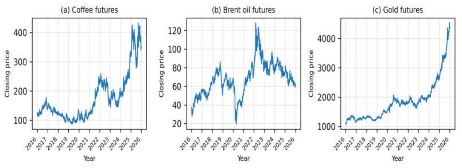
Figure 2.
Base-100 price index by commodity: (a) coffee; (b) Brent oil; (c) gold.
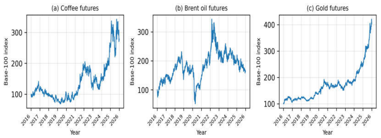
Figure 3.
Empirical distribution of logarithmic returns: (a) coffee; (b) Brent oil; (c) gold.
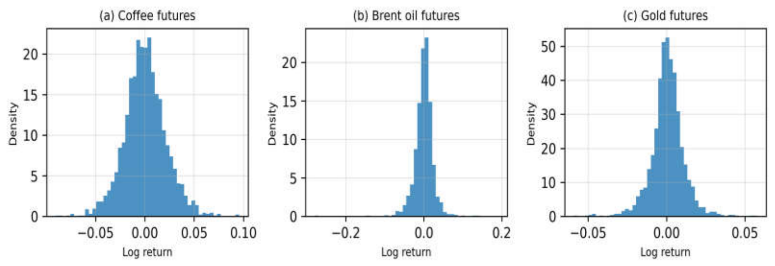
Figure 4.
30-day annualized rolling volatility: (a) coffee; (b) Brent oil; (c) gold.
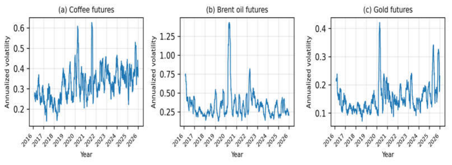
Figure 5.
Autocorrelation of returns and squared returns: (a) coffee; (b) Brent oil; (c) gold.
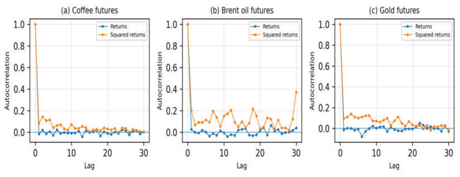
Figure 6.
DFA scaling curves on a log-log scale: (a) coffee; (b) Brent oil; (c) gold.
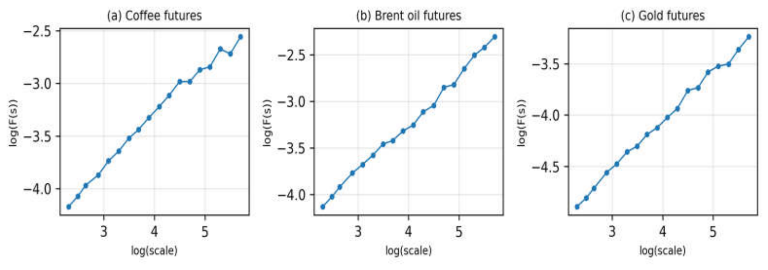
Figure 7.
Generalized MF-DFA functions: (a) coffee; (b) Brent oil; (c) gold.
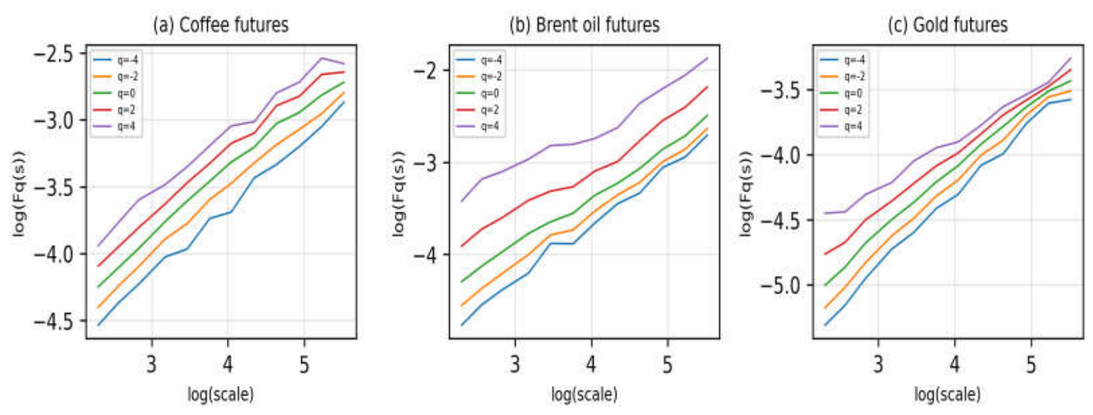
Figure 8.
Monte Carlo fan charts with P5-P95 intervals: (a) coffee; (b) Brent oil; (c) gold.
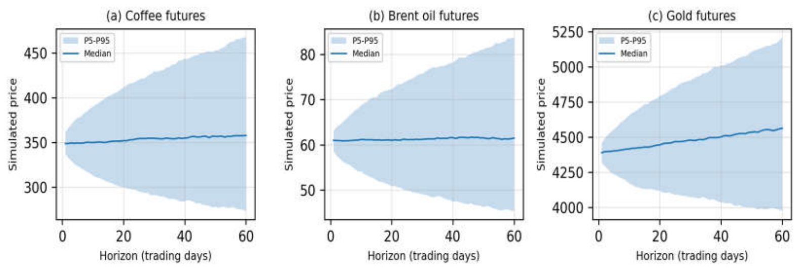

Table 1.
Dataset coverage and financial scope.
| Commodity | Category | Instrument | Quotation unit | Source | Start date | End date | Valid prices | Valid returns |
|---|---|---|---|---|---|---|---|---|
| Coffee | agricultural | Coffee futures | US cents/lb | Investing.com | 2016-01-04 | 2025-12-31 | 2516 | 2515 |
| Brent oil | energy | Brent oil futures | USD/bbl | Investing.com | 2016-01-04 | 2025-12-31 | 2582 | 2581 |
| Gold | precious metal / safe haven | Gold futures | USD/troy oz | Investing.com | 2016-01-04 | 2025-12-30 | 2188 | 2187 |
Table 2.
Quality-control and reproducibility checks applied to the dataset.
| Control | Field | Validation criterion | Scientific purpose |
|---|---|---|---|
| Temporal ordering | date, commodity | Ascending order within each commodity | Avoids calculating returns out of sequence |
| Duplicate control | date, commodity | No repeated dates for the same commodity | Guarantees unique observations |
| Positive prices | closing_price | Numeric values greater than zero | Allows logarithms to be applied |
| Return consistency | log_return | Valid returns = valid prices - 1 | Verifies internal calculation by series |
| No interpolation | date | Own calendars preserved | Avoids artificial smoothing of shocks |
| Volatility window | rolling_volatility_30d | Calculation only with sufficient window | Explains unavailable initial values |
| Traceability | source, notes | Source and processing notes preserved | Facilitates auditing and reuse |
Table 3.
Processed dataset variables and analytical function.
| Variable | Technical definition | Transformation | Analytical function |
|---|---|---|---|
| closing_price | Daily closing price of the futures contract | Original market record | Reconstruction of levels and nominal trajectory |
| log_price | Natural logarithm of the closing price | Scale homogenization and return preparation | |
| log_return | Continuous relative variation between two consecutive prices | Risk, dependence and distribution analysis | |
| abs_return | Absolute magnitude of the logarithmic return | Identification of fluctuation intensity | |
| squared_return | Squared logarithmic return | Evidence of second-moment persistence | |
| rolling_volatility_30d | 30-day annualized rolling volatility | Rolling standard deviation x | Reading of recent risk and stress episodes |
| base100_index | Index normalized from the first valid price | Accumulated comparison between assets with different units | |
| standardized_return | Return centered and scaled by its standard deviation | Detection of relative extremes by commodity |
Table 4.
Consistency between valid prices and returns.
| Commodity | Valid prices | Valid returns | Difference | Diagnosis |
|---|---|---|---|---|
| Coffee | 2516 | 2515 | 1 | Consistent |
| Brent oil | 2582 | 2581 | 1 | Consistent |
| Gold | 2188 | 2187 | 1 | Consistent |
Table 5.
Descriptive and diagnostic statistics of logarithmic returns.
| Commodity | N | Mean | SD | P1 | Median | P99 | Skew. | Kurt. | JB | Q(20) r | Q(20) r² | DFA H |
|---|---|---|---|---|---|---|---|---|---|---|---|---|
| Coffee | 2,515 | 0.00040 | 0.02102 | -0.0499 | 0.0000 | 0.0530 | 0.099 | 3.973 | 103.2 | 15.9 | 200.8 | 0.451 |
| Brent oil | 2,581 | 0.00019 | 0.02437 | -0.0673 | 0.0016 | 0.0619 | -1.092 | 20.742 | 34366.0 | 28.1 | 899.2 | 0.486 |
| Gold | 2,187 | 0.00064 | 0.01034 | -0.0272 | 0.0006 | 0.0289 | -0.196 | 6.645 | 1224.6 | 22.7 | 368.7 | 0.445 |
Table 6.
Empirical evidence of analytical reuse of the dataset.
| Analytical dimension | Observed evidence | Dataset variables | Scientific interpretation |
|---|---|---|---|
| Return distribution | High kurtosis and high Jarque-Bera statistics in the three markets | log_return, standardized_return | Returns preserve heavy tails and departure from normality |
| Volatility and recent risk | Differentiated episodes of rolling volatility and heterogeneous dispersion | abs_return, squared_return, rolling_volatility_30d | The database makes it possible to identify stress periods and compare risk intensity |
| Second-moment dependence | Q(20) on squared returns exceeds Q(20) on simple returns | log_return, squared_return | Dependence is more concentrated in variability than in the mean |
| Temporal scaling | Structured DFA curves and H values close to 0.5 with differences by commodity | log_return | The dataset is suitable for cautious temporal-dependence studies |
| Multifractal heterogeneity | Generalized fluctuation functions differ across q orders | log_return, abs_return, squared_return | Small and large fluctuations can be studied separately |
| Probabilistic simulation | Monte Carlo fan charts with differentiated P5-P95 bands | closing_price, log_return | The dataset supports risk scenarios and uncertainty intervals |
Disclaimer/Publisher’s Note: The statements, opinions and data contained in all publications are solely those of the individual author(s) and contributor(s) and not of MDPI and/or the editor(s). MDPI and/or the editor(s) disclaim responsibility for any injury to people or property resulting from any ideas, methods, instructions or products referred to in the content. |
© 2026 by the authors. Licensee MDPI, Basel, Switzerland. This article is an open access article distributed under the terms and conditions of the Creative Commons Attribution (CC BY) license (http://creativecommons.org/licenses/by/4.0/).
Copyright: This open access article is published under a Creative Commons CC BY 4.0 license, which permit the free download, distribution, and reuse, provided that the author and preprint are cited in any reuse.