

Submitted:
19 August 2026
Posted:
21 August 2026
You are already at the latest version
Abstract
Geopolitical uncertainty has become an increasingly relevant source of information for financial markets, yet whether it improves the out-of-sample forecasting of emerging-market stock returns remains unclear. This study examines whether geopolitical risk (GPR), together with global financial information, improves forecasts of Thai stock-market returns. Using monthly data from January 1990 to July 2026, the study compares ARIMA–GARCH and ARIMAX–GARCH benchmarks with Random Forest, XGBoost, and LightGBM across 1-, 3-, 6-, and 12-month forecasting horizons. An expanding-window rolling-origin framework is employed, with forecast accuracy evaluated using RMSE and MAE and statistical differences assessed using the Diebold–Mariano test and Model Confidence Set procedure. SHAP analysis is used to interpret predictor contributions. The results show that machine-learning models substantially outperform the econometric benchmarks, with LightGBM providing the most consistent forecasting performance across horizons. GPR contributes additional predictive information at the 1- and 3-month horizons, although its contribution weakens at longer horizons. GPR also emerges as the most influential predictor in the LightGBM model. The findings highlight the value of integrating geopolitical information into nonlinear forecasting frameworks for Thai stock-market returns.
Keywords:
geopolitical risk
; Thai stock market
; stock-market returns
; forecasting
; machine learning
; LightGBM
; GARCH
; out-of-sample forecasting
; explainable AI
1. Introduction
Geopolitical developments have become an increasingly relevant source of uncertainty for financial markets. Armed conflicts, trade disruptions, sanctions, energy-market disturbances, and changes in international relations can alter expectations about economic conditions and asset prices. For investors and financial institutions, the challenge is therefore not only to understand how geopolitical events affect financial markets, but also to determine whether geopolitical information can improve the forecasting of future market returns. This distinction is important because evidence of an association between geopolitical risk and financial outcomes does not necessarily imply useful out-of-sample predictive information.
The forecasting problem is particularly challenging for stock-market returns. Returns are affected simultaneously by their own historical dynamics and by information originating from commodity markets, exchange rates, global financial conditions, and investor expectations. These relationships may also be nonlinear and may change across forecast horizons. Recent developments in artificial intelligence and machine learning have consequently expanded the set of tools available for financial forecasting. A recent systematic review of AI-based financial forecasting confirms the rapid expansion of machine-learning applications across equity, commodity, foreign-exchange, and cryptocurrency markets, while emphasizing the importance of nonlinear modeling and rigorous out-of-sample evaluation [1].
1.1. Why Thailand?
The Thai stock market provides a particularly relevant setting for examining the forecasting value of geopolitical information. Thailand is an open emerging economy whose financial market is closely connected with international trade, tourism, energy markets, commodity prices, exchange-rate movements, and cross-border capital flows. Consequently, external geopolitical developments can reach the domestic equity market through several channels rather than through domestic political conditions alone.
The relevance of external uncertainty to Thailand is also supported by recent evidence. For example, research on political uncertainty in the Thai economy finds that political events can have heterogeneous effects on firm-level financial performance and market value, illustrating the sensitivity of Thai financial outcomes to uncertainty-related conditions. More broadly, Thailand's position within regional and global financial networks makes it useful for testing whether geopolitical information contains incremental predictive information for an emerging-market equity index.
The choice of Thailand also addresses an important empirical issue. Evidence obtained from large developed markets cannot automatically be generalized to emerging markets because market depth, investor composition, external dependence, and transmission mechanisms differ across economies. Recent research on emerging-market forecasting similarly emphasizes that model performance and predictor importance can depend on the characteristics of the market being forecast. A recent study of New Zealand, for example, demonstrates the value of combining global intermarket information with econometric and machine-learning forecasting methods in an emerging-market setting.
Accordingly, the Thai Stock Exchange (SET) provides an informative case for evaluating whether geopolitical and global financial information can improve out-of-sample forecasts of stock-market returns, rather than merely explaining historical market movements.
1.2. From Explanation to Forecasting
The present study deliberately focuses on forecasting rather than causal estimation. The central issue is whether information available at the forecast origin can improve predictions of future RSET returns. This perspective is consistent with the recent movement in financial research toward strict walk-forward and out-of-sample evaluation. Forecasting studies increasingly distinguish predictive performance from in-sample explanatory power, particularly when models are flexible enough to capture complex relationships.
This distinction is especially important when comparing conventional econometric models with machine-learning algorithms. A model may provide a good statistical description of historical returns without necessarily producing superior forecasts. Conversely, a flexible nonlinear model may improve predictive accuracy without providing a structural or causal interpretation. The present study therefore evaluates both forecast accuracy and statistical evidence of predictive superiority, rather than relying on in-sample fit alone.
Recent methodological work reinforces the importance of this approach. Naifar [2], for example, combines conventional financial predictors, geopolitical risk, multiple machine-learning models, Diebold–Mariano tests, Model Confidence Set analysis, and SHAP explainability to distinguish numerical forecasting performance from statistically supported model differences.
1.3. Research Objectives
Against this background, this study has four objectives:
- To evaluate whether geopolitical risk and selected global financial indicators provide useful information for forecasting Thai stock-market returns.
- To compare the out-of-sample forecasting performance of conventional volatility-aware econometric models and nonlinear machine-learning models.
- To examine whether model performance and the predictive value of geopolitical information vary across short-, medium-, and longer-term forecast horizons.
- To identify the predictors that contribute most strongly to the forecasts generated by the best-performing machine-learning model using explainable machine learning.
These objectives are deliberately framed around predictive performance, rather than causal effects. The study therefore does not attempt to estimate whether geopolitical risk causes changes in Thai stock returns. Instead, it asks whether geopolitical information contains incremental forecasting information when combined with market and global financial variables.
1.4. Research Questions
The empirical analysis addresses four corresponding research questions:
RQ1. Does incorporating geopolitical risk and global financial information improve the out-of sample forecasting of Thai stock-market returns?
RQ2. Do nonlinear machine-learning models outperform ARIMA–GARCH and ARIMAX–GARCH benchmarks in forecasting RSET returns?
RQ3. Does the relative forecasting performance of the competing models vary across 1-, 3-, 6-, and 12-month horizons?
RQ4. Which geopolitical, market, commodity, and exchange-rate variables contribute most strongly to the predictions of the best-performing machine-learning model?
These questions provide a direct link between the motivation of the study and the empirical design. They also avoid presuming that geopolitical risk must improve forecasts or that one particular machine-learning algorithm must dominate.
1.5. Empirical Strategy and Contribution
To answer these questions, the study uses monthly Thai stock-market return data together with the Geopolitical Risk Index and selected global financial indicators. The empirical framework compares ARIMA–GARCH and ARIMAX–GARCH models with Random Forest, XGBoost, and LightGBM. Forecasts are generated using an expanding-window rolling-origin procedure at 1-, 3-, 6-, and 12-month horizons. Forecast performance is evaluated using RMSE and MAE, while the Diebold–Mariano test and Model Confidence Set procedure are used to distinguish numerical differences from statistically supported differences in predictive accuracy. SHAP analysis is subsequently used to interpret the contribution of individual predictors.
The contribution of the study is therefore methodological and empirical. Empirically, it provides evidence on the forecasting value of geopolitical and global financial information for the Thai equity market. Methodologically, it evaluates conventional and nonlinear forecasting approaches within a common information set and out-of-sample framework, while combining predictive-accuracy measures, formal statistical comparison, and explainable machine learning. This integrated design is particularly relevant given recent evidence that no forecasting algorithm necessarily dominates across all assets, horizons, and loss functions.
The study also contributes to the emerging-market forecasting literature by focusing on Thailand, an economy exposed to international commodity, exchange-rate, trade, and geopolitical developments. Rather than assuming that evidence from major developed markets applies directly to Thailand, the analysis provides a market-specific test of whether geopolitical information has incremental predictive value.
1.6. Structure of the Paper
The remainder of the paper is organized as follows. Section 2 reviews the literature on geopolitical risk, financial-market predictability, machine-learning forecasting, and explainable machine learning, and identifies the research gap addressed by the study. Section 3 describes the data, unit-root analysis, econometric and machine-learning models, forecasting design, statistical evaluation procedures, and SHAP methodology. Section 4 presents the estimation results, out-of-sample forecasting performance, statistical model comparisons, SHAP results, discussion, and robustness analysis. Section 5 concludes the study and discusses limitations, future research, and policy and investment implications.
2. Literature Review
2.1. Geopolitical Risk and Financial Market Predictability
Geopolitical risk (GPR) has become an increasingly important source of uncertainty for financial markets because geopolitical conflicts can affect investor sentiment, international trade, energy markets, capital flows, and expectations about future economic conditions. The news-based GPR index developed by Caldara and Iacoviello [3] has provided a systematic measure of geopolitical uncertainty and has facilitated a growing empirical literature examining its effects across financial assets.
Early evidence indicates that geopolitical risk can affect both returns and volatility, although the magnitude and direction of the effects vary across markets and episodes. More recent studies emphasize that geopolitical risk should not necessarily be interpreted as having a constant linear effect. For example, evidence from global stock markets indicates that the relationship between geopolitical risk and returns can vary across market conditions and the conditional distribution of returns. Enescu and Răileanu Szeles [4] find that geopolitical risk is associated with negative stock-market effects during bullish conditions but can exhibit a positive association during bearish market states, with stronger effects in emerging and commodity-rich markets.
This regime dependence is particularly relevant for emerging markets, where external shocks can transmit through exchange rates, commodity prices, foreign capital flows, and investor sentiment. Recent evidence for China also shows that geopolitical-risk exposure contains information about subsequent stock returns. Zhang et al. [5] document a significant low-GPR-exposure premium in Chinese stocks, suggesting that geopolitical risk can influence return predictability beyond conventional risk factors.
The literature therefore suggests that GPR contains economically relevant information for financial markets, but the predictive relationship is neither necessarily linear nor stable across horizons and market conditions. This observation motivates the use of forecasting frameworks capable of accommodating nonlinearities and changing predictor importance.
2.2. Geopolitical Risk and Forecasting
A related strand of research focuses explicitly on whether geopolitical risk improves out-of-sample forecasting rather than merely explaining contemporaneous returns or volatility. This distinction is important because statistical significance in an explanatory model does not necessarily imply economically useful predictive information.
Plakandaras et al. [6] were among the early studies to examine the forecasting role of geopolitical uncertainty using machine-learning methods. Using data for 14 emerging economies, they evaluated geopolitical risk as a predictor of oil prices, exchange rates, stock-market indices, and gold prices across multiple forecast horizons. Their results indicate that the predictive role of geopolitical risk is generally limited for several assets but more evident for gold, highlighting the asset-specific nature of geopolitical-risk transmission.
More recent research provides stronger evidence that the predictive value of GPR depends on the forecasting environment. Schlosky et al. [7], for example, show that geopolitical risk affects the forecasting ability of standard predictors for U.S. stock returns. Importantly, forecasting performance is significantly better during periods of high geopolitical risk, suggesting that the information content of predictors is state dependent rather than constant over time.
Rafi and Ali [8] further extend this literature by decomposing geopolitical risk into geopolitical threat and geopolitical act components across 40 countries. Their results indicate that geopolitical threat factors have broader predictive power than geopolitical act factors, with significant one-month predictability found across a substantial proportion of countries and positive out-of-sample predictive gains in many markets.
These findings indicate that the forecasting value of geopolitical risk can depend on the type of geopolitical information, market, and forecast horizon. Consequently, a useful empirical framework should evaluate forecasting performance at multiple horizons rather than rely on a single forecast period.
2.3. Machine Learning and Stock Return Forecasting
Traditional econometric models remain important benchmarks in financial forecasting because they provide interpretable structures for serial dependence and conditional volatility. However, financial returns may exhibit nonlinear relationships, interactions, structural changes, and time-varying predictive information that are difficult to capture using fixed parametric specifications.
The development of machine-learning methods has therefore expanded the forecasting literature. Reviews of financial forecasting research indicate substantial growth in the use of machine-learning and deep-learning approaches, particularly because these methods can accommodate nonlinear relationships and high-dimensional predictor sets [9,10].
Recent empirical evidence also supports the usefulness of machine learning for return predictability. Cakici and Zaremba [11] show that machine-learning models can identify significant return predictability across countries, although the importance of individual predictors varies across forecast horizons. Their findings also suggest that predictive relationships may be concentrated in a relatively small number of characteristics rather than being uniformly distributed across all predictors.
Similarly, recent evidence from Risks shows that machine-learning models can improve the modeling of stock returns relative to conventional regression-based approaches when nonlinear risk-factor relationships are considered. The results emphasize that machine learning can reveal predictive structures that may not be captured adequately by standard linear specifications.
However, the literature also indicates that no single machine-learning algorithm is universally superior. Forecasting performance depends on the asset, predictors, horizon, and evaluation design. This reinforces the importance of comparing multiple algorithms using strictly out-of-sample procedures rather than selecting a model based solely on in-sample fit.
2.4. Explainable Machine Learning and Geopolitical Risk
An important limitation of machine-learning forecasting is that predictive improvement alone does not explain why a model performs well. This has motivated the increasing use of explainable artificial intelligence, particularly SHAP-based methods, to identify the contribution of individual predictors.
Niu et al. [12] provide particularly relevant evidence by combining geopolitical-risk categories, machine-learning forecasting, and SHAP analysis. Their study finds that military build-ups and war escalation are among the most important geopolitical-risk components for forecasting U.S. stock-market volatility. The study also demonstrates the usefulness of SHAP for identifying which geopolitical variables contribute most strongly to predictive performance.
More recent work has extended this approach to financial forecasting. Naifar [2], published in Forecasting, combines geopolitical risk and supply-chain stress with machine-learning models, SHAP explainability, Diebold–Mariano tests, and Model Confidence Set analysis. The study finds that the forecasting value of geopolitical risk is asset specific and that nonlinear models do not uniformly dominate across all assets and loss functions. Importantly, the paper demonstrates the value of combining forecast evaluation, statistical model comparison, and explainability rather than treating machine-learning accuracy as the only criterion.
This methodological development is highly relevant to the present study because it moves the literature from the question of whether geopolitical risk predicts financial markets toward the more informative questions of when, at what horizon, through which variables, and with which nonlinear model geopolitical information contributes to forecasting performance.
2.5. Research Gap and Contribution
The literature provides substantial evidence that geopolitical risk contains information relevant to financial markets, but several gaps remain.
First, much of the literature examines individual relationships between GPR and returns or volatility, whereas fewer studies directly compare geopolitical-risk forecasting models with conventional econometric benchmarks across multiple forecast horizons.
Second, although machine learning is increasingly used in financial forecasting, relatively limited evidence combines traditional ARIMA–GARCH/ARIMAX–GARCH benchmarks with multiple tree-based machine-learning models under a common rolling-origin forecasting framework.
Third, the predictive value of geopolitical risk appears to be horizon dependent, but relatively few studies jointly evaluate short-, medium-, and longer-horizon forecasts using formal statistical comparison procedures.
Fourth, machine-learning studies increasingly use explainability tools, but the integration of SHAP, Diebold–Mariano testing, and Model Confidence Set analysis remains relatively limited in emerging-market stock-return forecasting.
Finally, evidence for Thailand remains comparatively limited. Existing international studies provide useful evidence that geopolitical risk affects financial markets, but the extent to which GPR contributes to the out-of-sample predictability of Thai stock-market returns, particularly relative to nonlinear machine-learning models and across multiple forecast horizons, remains insufficiently established.
The present study addresses these gaps by comparing ARIMA–GARCH and ARIMAX–GARCH benchmarks with Random Forest, XGBoost, and LightGBM models using an expanding-window out-of-sample forecasting framework. Forecast horizons of 1, 3, 6, and 12 months are considered, while Diebold–Mariano tests and the Model Confidence Set are used to evaluate statistical differences in predictive performance. Finally, SHAP analysis is employed to identify the predictors contributing most strongly to the forecasts. This integrated framework allows the study to evaluate not only whether geopolitical and financial information improves forecasting, but also which model performs best, whether the advantage is statistically significant, whether it persists across horizons, and which predictors drive the nonlinear forecasts.
3. Methodology and Data Collection
3.1. Data Collection and Variable Definition
This study examines the predictability of Thai stock-market returns using geopolitical risk and global financial indicators. The monthly sample covers January 1990 to July 2026, comprising 439 observations. The dependent variable is the monthly return of the Stock Exchange of Thailand (RSET). The explanatory variables include the Geopolitical Risk Index (GPR), Brent crude oil returns (RBRENT), gold returns (RGOLD), and U.S. dollar index returns (RDXY). The GPR measure follows the news-based geopolitical risk index developed by Caldara and Iacoviello [3]. All price-based financial variables are transformed into continuously compounded returns to improve comparability across series and to provide a consistent basis for time-series modeling.
Stock-Market Return: The monthly return of the Stock Exchange of Thailand (SET) Index is calculated as the continuously compounded return:
where denotes the SET Index at month. The resulting series is the dependent variable in all forecasting models.
Geopolitical Risk: Geopolitical risk is measured using the Geopolitical Risk Index (GPR). Unlike the price-based financial variables, GPR is used in its original index form and is not transformed into a return. The index captures changes in geopolitical tensions and uncertainty and is included as an external predictor in the ARIMAX-GARCH and machine-learning models.
Brent Crude-Oil Return: International oil-market conditions are represented by the Brent crude-oil price. The monthly Brent return is calculated as:
where denotes the Brent crude-oil price at month.
Gold Return: Gold-market conditions are represented by the international gold price. The monthly gold return is calculated as:
where denotes the international gold price at month.
U.S. Dollar Index Return: Global currency-market conditions are represented by the U.S. Dollar Index (DXY). The monthly return of the U.S. Dollar Index is calculated as:
where denotes the U.S. Dollar Index at month.
Lagged Stock-Market Returns: To capture the temporal dependence of stock-market returns, the machine-learning models include the first 12 lags of the SET return:
Thus, the machine-learning feature set contains, together with GPR, RBRENT, RGOLD, and RDXY.
Model-Specific Predictor Sets
The benchmark ARIMA-GARCH model captures the dynamics of the SET return series through its autoregressive and moving-average structure without incorporating external predictors. The ARIMAX-GARCH model extends the benchmark specification by incorporating geopolitical risk and global financial-market variables as external predictors. The machine-learning models—Random Forest, XGBoost, and LightGBM—use a common feature set consisting of the first 12 lags of RSET, GPR, RBRENT, RGOLD, and RDXY. This common feature specification allows the predictive performance of the three machine-learning algorithms to be compared under the same information set.
The machine-learning feature vector can be expressed as:
Information Availability
To prevent look-ahead bias, all predictors used for forecasting are restricted to information available at or before the forecast origin. For the machine-learning models, the lagged RSET variables are constructed from previously observed returns, while the external financial and geopolitical variables are incorporated according to the information set defined in the forecasting design. The same information constraint is imposed consistently across all forecasting models (Table 1).
Model Information Set
| Predictor | ARIMA-GARCH | ARIMAX-GARCH | Random Forest | XGBoost | LightGBM |
| SET return dynamics | ✓ | ✓ | ✓ | ✓ | ✓ |
| — | ✓ | ✓ | ✓ | ✓ | |
| — | ✓ | ✓ | ✓ | ✓ | |
| — | ✓ | ✓ | ✓ | ✓ | |
| — | ✓ | ✓ | ✓ | ✓ | |
| —* | —* | ✓ | ✓ | ✓ | |
| as machine-learning features. The machine-learning models use the same feature set across Random Forest, XGBoost, and LightGBM. | |||||
3.2. Descriptive Statistics
Table 2 reports the descriptive statistics of the variables used in the forecasting analysis. The RSET return series has a mean close to zero but exhibits substantial dispersion and excess kurtosis, indicating the presence of large return movements and non-normality. Brent crude oil returns display the highest standard deviation among the financial return variables and pronounced excess kurtosis, while gold and U.S. dollar returns also depart from normality. The GPR index exhibits particularly strong positive skewness and excess kurtosis, indicating that geopolitical risk is characterized by occasional but exceptionally large spikes. The Jarque–Bera statistics reject normality for all variables at conventional significance levels. These distributional characteristics provide useful motivation for considering both volatility-aware econometric benchmarks and nonlinear machine-learning models in the forecasting analysis.
3.3. Preliminary Analysis and Unit Root Tests
The stationarity of the variables was examined using the Augmented Dickey–Fuller (ADF), Phillips–Perron (PP), and KPSS tests. The tests were used as complementary checks because the ADF and PP tests have a unit-root null hypothesis, whereas the KPSS test has a stationarity null hypothesis [13,14,15]. The results are reported in Table 3 and confirm the time-series properties used in the subsequent forecasting analysis.
3.4. Econometric Model Specification
3.4.1. ARIMA–GARCH Benchmark Model
The ARIMA framework is used to model the conditional mean of RSET returns. The general ARIMA specification is:
where denotes the backshift operator, is the order of differencing, and and are the autoregressive and moving-average polynomials, respectively [16].
To account for time-varying volatility, the conditional variance follows a GARCH(1,1) specification:
where is the variance intercept, captures the response of volatility to recent shocks, and represents volatility persistence [17,18]. Standardized Student-t innovations are assumed to accommodate heavy-tailed financial returns.
3.4.2. ARIMAX–GARCH Model
To examine whether geopolitical and global financial information provides additional predictive information, the conditional mean equation is extended with exogenous variables:
where
The conditional variance is specified as:
The use of lagged predictors ensures that the model relies only on information available before the forecast period. The GPR measure follows Caldara and Iacoviello [3]. The ARIMA orders are selected using an exhaustive search based on the corrected Akaike information criterion (AICc), followed by rolling out-of-sample evaluation.
3.5. Machine Learning Models
Three tree-based machine-learning models are employed: Random Forest, XGBoost, and LightGBM. These models allow nonlinear relationships and interactions among predictors to be captured without imposing a specific linear functional form.
3.5.1. Random Forest
Random Forest combines predictions from multiple regression trees. The resulting prediction can be represented as:
where denotes the prediction from the -th regression tree and is the number of trees [19].
3.5.2. XGBoost
XGBoost constructs an additive ensemble of regression trees by minimizing a loss function with a regularization term:
where represents the prediction loss and controls model complexity:
The regularization component helps control model complexity and reduce overfitting [20].
3.5.3. LightGBM
LightGBM uses a gradient-boosting decision-tree framework. The prediction is represented as an additive function of individual trees:
The model uses an efficient tree-learning strategy to capture nonlinear relationships and interactions among predictors [21].
For all machine-learning models, the predictor set consists of twelve lags of RSET together with GPR, RBRENT, RGOLD, and RDXY. Models are estimated separately at each forecast origin using only information available at that point in time.
3.6. Forecasting Design
An expanding-window rolling-origin forecasting scheme is employed to provide a consistent and strictly out-of-sample comparison across all competing models. At each forecast origin, the estimation sample is expanded by one observation, and the models are re-estimated using only information available up to that point in time [22].
The full sample contains 439 monthly observations from January 1990 to July 2026. The initial estimation window comprises 307 observations, covering January 1990 to July 2015. Accordingly, the first out-of-sample forecast is generated for August 2015. The estimation window is subsequently expanded by one observation at each forecast origin, and the competing models are re-estimated sequentially.
Forecasts are generated at four horizons: one-, three-, six-, and twelve-month ahead. Because the forecast horizons differ, the number of available forecast origins varies across horizons. To maintain a common evaluation endpoint, all forecasts are evaluated against realized observations through July 2026. Consequently, the final forecast origin differs across horizons according to the corresponding forecast horizon.
The forecasting information set is restricted to information available at each forecast origin. For the econometric models, the external predictors enter with a one-month lag, while the machine-learning models use the same underlying lagged information structure together with twelve lags of RSET. This common information constraint is imposed to prevent look-ahead bias and to ensure that differences in forecasting performance reflect differences in model structure rather than differences in information availability.
The resulting forecasting design is summarized in Table 4.
3.7. Forecast Evaluation and Statistical Comparison
Forecast accuracy is evaluated using the root mean squared error (RMSE) and mean absolute error (MAE), calculated from the complete set of observation-level out-of-sample forecasts. These measures are reported separately for each competing model and forecast horizon. Lower values of RMSE and MAE indicate better predictive performance.
The RMSE and MAE are defined as:
where denotes the forecast error, denotes the realized return, denotes the corresponding out-of-sample forecast, and denotes the number of out-of-sample forecasts.
The Diebold–Mariano (DM) test is used to assess whether differences in predictive accuracy between competing models are statistically significant [23]. The loss differential is defined as:
where squared-error loss is used:
The DM statistic is based on the mean loss differential and its estimated long-run variance. The test is conducted separately for the 1-, 3-, 6-, and 12-month forecasting horizons.
Because pairwise comparisons do not necessarily identify the set of models that are statistically indistinguishable from the best-performing models, the Model Confidence Set (MCS) procedure is additionally employed [24]. The MCS is estimated separately for each forecast horizon using squared-error loss at the 10% significance level. The procedure identifies the subset of models that cannot be statistically distinguished from the superior forecasting models.
Accordingly, the forecasting evaluation proceeds in three complementary stages. First, RMSE and MAE are used to describe the numerical forecasting performance of each model. Second, the DM test is used to assess pairwise statistical differences in predictive accuracy. Third, the MCS procedure is used to identify the set of models that remain statistically competitive at the specified confidence level.
This evaluation framework distinguishes numerical differences in forecast accuracy from statistically supported differences in predictive performance and provides a consistent basis for comparing econometric and machine-learning models across forecasting horizons.
3.8. Explainable Machine Learning: SHAP
Following the out-of-sample forecasting evaluation, SHAP (SHapley Additive exPlanations) is employed to interpret the predictions generated by the best-performing machine-learning model, LightGBM. SHAP provides an additive decomposition of each model prediction into a baseline component and feature-specific contributions [25].
SHAP decomposes each prediction into a baseline component and feature-specific contributions (Lundberg & Lee, 2017):
where represents the baseline prediction and represents the contribution of the predictor. Mean absolute SHAP values are used to assess global feature importance, while SHAP dependence plots are used to examine the relationship between individual predictors and their contributions to model predictions.
The SHAP framework is used to examine both the relative importance and directional contribution of individual predictors. Mean absolute SHAP values are used to assess global feature importance, while SHAP dependence plots are employed to examine how changes in selected predictors are associated with their contributions to the model's predicted RSET return.
The interpretation focuses on identifying which geopolitical, market, commodity, exchange-rate, and lagged-return variables contribute most strongly to the LightGBM forecasts. Importantly, SHAP values are interpreted as predictive contributions rather than causal effects. A large SHAP contribution indicates that a predictor is important for the model's prediction but does not imply that changes in the predictor causally determine subsequent stock-market returns.
4. Results and Discussion
4.1. Results
4.1.1. ARIMA and ARIMA–GARCH Benchmark Models
To establish benchmark models for forecasting Thai stock-market returns, we first estimated a non-seasonal autoregressive integrated moving average (ARIMA) model using the monthly SET return series (RSET). Since RSET is already expressed as a return series, no additional differencing was imposed. The ARIMA specification was selected through an exhaustive search over alternative model orders as reported in Table 5 using the corrected Akaike information criterion (AICc), with both stepwise search and approximation disabled. The procedure selected an ARIMA(3,0,2) model with zero mean, which yielded the lowest AICc (−989.41).
The residual diagnostics indicated no significant remaining serial correlation, as shown by the Ljung–Box test (Q = 22.918, p = 0.241). However, the ARCH LM test strongly rejected the null hypothesis of no conditional heteroskedasticity (χ² = 57.994, p < 0.001), indicating time-varying volatility in RSET.
To account for this conditional heteroskedasticity, we subsequently estimated an ARIMA(3,0,2)–GARCH(1,1) model with Student-t innovations. The estimated ARCH and GARCH parameters were statistically significant (α₁ = 0.151, p = 0.008; β₁ = 0.837, p < 0.001), with high volatility persistence (α₁ + β₁ = 0.988). Diagnostic tests based on the standardized residuals found no evidence of remaining serial correlation or ARCH effects. The Student-t shape parameter was also statistically significant (p < 0.001).
The ARIMA–GARCH model was therefore retained as a volatility-aware benchmark for the subsequent out-of-sample forecasting analysis. Importantly, the final comparison of forecasting performance is based on rolling out-of-sample forecasts rather than in-sample information criteria alone.
Figure 1 displays the standardized residuals, which show no evident serial dependence, while the autocorrelation of squared standardized residuals is largely contained within the confidence bounds, supporting the adequacy of the conditional variance specification.
4.1.2. ARIMAX–GARCH Model with Geopolitical and Financial Predictors
To examine whether geopolitical and global financial information provides additional predictive information for Thai stock-market returns, the benchmark framework was extended by incorporating lagged geopolitical and financial-market variables into the ARIMA specification. The information set consists of the one-month lagged Geopolitical Risk Index (GPR), Brent crude oil returns (RBRENT), gold returns (RGOLD), and U.S. dollar index returns (RDXY). Using lagged predictors ensures that the model relies only on information available prior to the forecast period.
An exhaustive AICc-based search selected an ARIMAX(2,0,2) specification, with an AICc of −994.35. The resulting residuals showed no significant serial correlation according to the Ljung–Box test (Q = 21.229, p = 0.384). However, the ARCH LM test remained significant (χ² = 51.691, p < 0.001), indicating that incorporating the external predictors did not eliminate the conditional heteroskedasticity identified in the benchmark model. Therefore, the conditional variance was subsequently modeled using a GARCH(1,1) process with Student-t innovations.
Table 6 reports the estimated coefficients and diagnostic statistics for the resulting ARIMAX(2,0,2)–GARCH(1,1) specification. The autoregressive and moving-average parameters are statistically significant, indicating persistent dynamic dependence in RSET. The volatility parameters are also significant, with α₁ = 0.140 (p = 0.011) and β₁ = 0.844 (p < 0.001), yielding high volatility persistence of α₁ + β₁ = 0.984. The diagnostic statistics reported in Table 6 indicate no evidence of remaining serial correlation or ARCH effects in the standardized residuals. The joint sign-bias test is also insignificant (p = 0.556), providing no evidence of unmodeled asymmetric effects.
Regarding the external predictors, the lagged Brent return is statistically significant and negatively associated with subsequent RSET (β = −0.072, p = 0.029), whereas the lagged GPR coefficient is positive and marginally significant at the 10% level (β = 0.000105, p = 0.052). The coefficients of lagged gold and U.S. dollar index returns are not statistically significant. These estimates are interpreted as predictive associations rather than causal effects.
Overall, the results in Table 6 support the adequacy of the ARIMAX–GARCH specification as an exogenous, volatility-aware benchmark. The model is therefore retained for the subsequent rolling out-of-sample forecasting evaluation, where its predictive performance is compared with the benchmark and machine-learning models.
4.1.3. Out-of-Sample Forecasting Performance
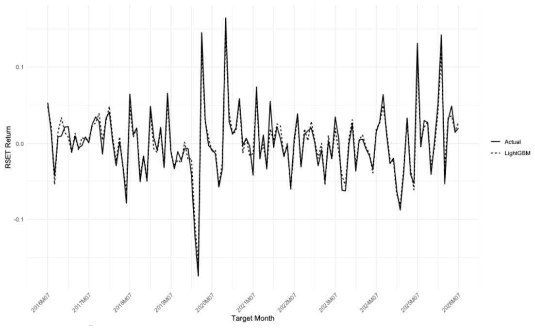
To provide a visual assessment of forecast performance, Appendix A presents plots comparing the actual RSET returns with the LightGBM forecasts at the 1-, 3-, 6-, and 12-month horizons. These plots provide a visual complement to the numerical accuracy measures reported in Table 7.
For completeness, the underlying observation-level forecasts are reported in Appendix C. Tables C1–C4 present the actual RSET returns together with the corresponding forecasts generated by the competing models across the different forecast horizons. Table C5 reports the corresponding Diebold–Mariano comparisons. The detailed forecast records in Tables C1–C4 provide the underlying observations from which the RMSE and MAE values reported in Table 7 are calculated.
At the one-month horizon, LightGBM achieves the lowest RMSE and MAE, with values of 0.0107 and 0.0081, respectively. At the 3- and 6-month horizons, XGBoost provides the best forecasting performance, with RMSE values of 0.0113 and 0.0110, respectively. At the 12-month horizon, LightGBM again records the lowest forecasting errors, with an RMSE of 0.0103 and an MAE of 0.0080.
Overall, the results demonstrate that nonlinear machine-learning models provide more accurate forecasts than the conventional econometric benchmarks, although the best-performing machine-learning model varies across forecast horizons.
To determine whether the observed differences in forecasting accuracy are statistically significant, the Diebold–Mariano (DM) test was conducted between the best-performing machine-learning model at each horizon and the ARIMA-GARCH benchmark. The results indicate that the forecasting improvements are statistically significant across all four horizons. The DM statistics based on RMSE loss are −4.472, −3.634, −3.936, and −2.706 for the 1-, 3-, 6-, and 12-month horizons, respectively, with corresponding p-values below 0.01. Similar results are obtained using MAE loss. These findings indicate that the superior forecasting performance of the machine-learning models is statistically significant rather than attributable to sampling variation alone.
4.1.4. Statistical Comparison of Forecast Accuracy
To further examine pairwise differences in predictive accuracy, Table 8 reports the Diebold–Mariano tests comparing LightGBM with the other competing models. LightGBM significantly outperforms both ARIMA-GARCH and ARIMAX-GARCH at all forecasting horizons, with p-values below 0.01. The same result is obtained against Random Forest, with statistically significant differences at all four horizons.
In contrast, the difference between LightGBM and XGBoost is statistically significant only at the 1-month horizon. At the 3-, 6-, and 12-month horizons, the null hypothesis of equal predictive accuracy cannot be rejected. Thus, although LightGBM remains statistically competitive across all horizons, XGBoost achieves lower numerical RMSE at the 3- and 6-month horizons.
4.1.5. Model Confidence Set Results
Table 9 reports the Model Confidence Set results across the four forecasting horizons. At the 10% significance level, LightGBM remains in the Superior Set of Models at all horizons. XGBoost is eliminated at the one-month horizon but remains in the Superior Set at the 3-, 6-, and 12-month horizons. In contrast, ARIMA-GARCH, ARIMAX-GARCH, and Random Forest are eliminated at all horizons.
These findings reinforce the results from the point-forecast measures and the Diebold–Mariano tests. LightGBM is the only model consistently retained across all forecasting horizons, while XGBoost represents a statistically competitive alternative at medium- and longer-term horizons.
4.1.6. Interpretation of the Best-Performing Model
Given that LightGBM is the only model retained in the Model Confidence Set across all four forecasting horizons, it was selected for further interpretation using SHAP analysis. Figure 2 shows the global importance of the predictors. GPR has the largest mean absolute SHAP value, followed by RSET_l8, RSET_l11, and RSET_l5. These results indicate that geopolitical risk and recent lagged dynamics of the Thai stock market are particularly important contributors to the LightGBM forecasts.
Additional SHAP-based results are reported in Appendix B. Appendix B provides the complete predictor ranking and further interpretation of the SHAP results, complementing the summary SHAP figures presented in the main text.
Figure 2.
Global feature importance of the LightGBM model based on mean absolute SHAP values. Note: Features are ranked according to their mean absolute SHAP values. Larger values indicate greater average contributions to the LightGBM predictions.
Figure 2.
Global feature importance of the LightGBM model based on mean absolute SHAP values. Note: Features are ranked according to their mean absolute SHAP values. Larger values indicate greater average contributions to the LightGBM predictions.
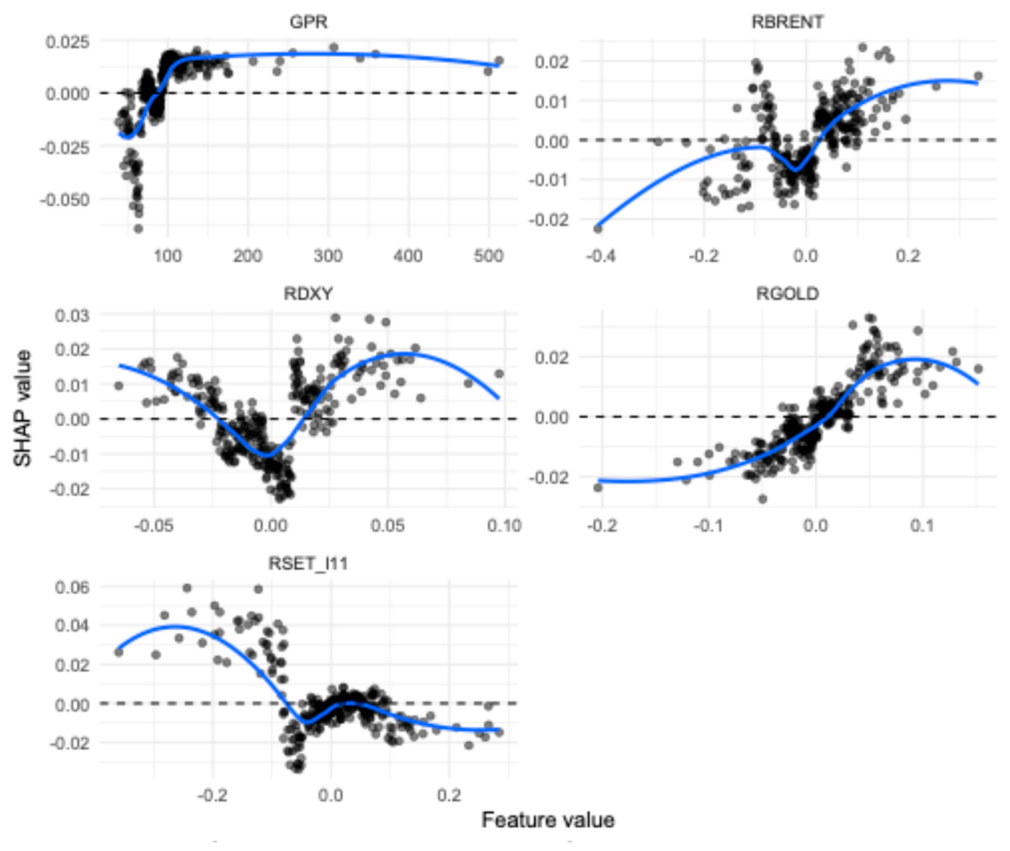
Figure 3.
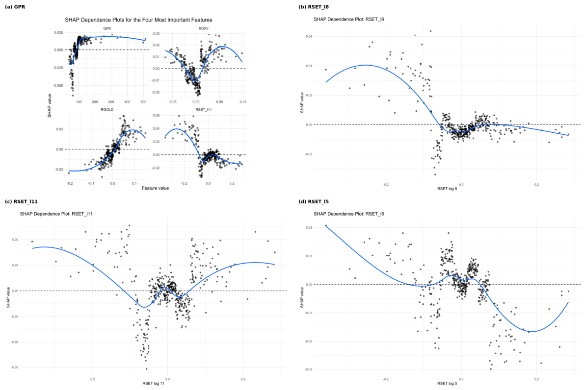
SHAP dependence plots for the four most influential predictors: (a) GPR, (b) RSET_l8, (c) RSET_l11, and (d) RSET_l5.
Figure 3.
SHAP dependence plots for the four most influential predictors: (a) GPR, (b) RSET_l8, (c) RSET_l11, and (d) RSET_l5.
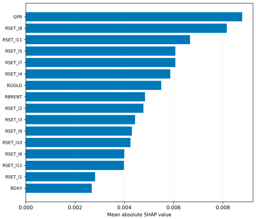
Figure 3.
illustrates nonlinear relationships between the four most influential predictors and their SHAP contributions to predicted RSET returns. The dependence patterns vary across the observed ranges of the predictors, indicating that the contribution of these variables is not adequately represented by a simple linear relationship. This nonlinear structure provides an interpretive explanation for the strong forecasting performance of LightGBM.
Figure 3.
illustrates nonlinear relationships between the four most influential predictors and their SHAP contributions to predicted RSET returns. The dependence patterns vary across the observed ranges of the predictors, indicating that the contribution of these variables is not adequately represented by a simple linear relationship. This nonlinear structure provides an interpretive explanation for the strong forecasting performance of LightGBM.
4.2. Discussion
4.2.1. Forecasting Value of Geopolitical and Financial Information
The results indicate that geopolitical and global financial information contains useful predictive information for Thai stock-market returns. This finding is consistent with recent evidence that geopolitical risk affects the predictability of equity returns and financial-market volatility. Schlosky et al. [7] show that geopolitical risk changes the out-of-sample forecasting performance of standard stock-return predictors, while Rafi and Ali [8] document significant out-of-sample predictability associated with geopolitical-risk factors across a broad set of international equity markets.
The present study extends this literature by examining the predictive value of geopolitical risk jointly with global commodity and exchange-rate information for the Thai stock market. Rather than treating geopolitical risk only as a source of market shocks, the findings demonstrate its usefulness as part of an information set for forecasting future RSET returns. This distinction is important because the evidence concerns predictive association rather than causality.
4.2.2. Why Nonlinear Forecasting Provides an Advantage
The superior performance of the machine-learning models suggests that the relationship between geopolitical conditions, global financial variables, and stock returns is unlikely to be adequately represented by a fixed linear specification. This interpretation is consistent with Niu et al. [12], who find that machine-learning methods improve out-of-sample forecasting of stock-market volatility when geopolitical-risk information is incorporated. Their results also show that geopolitical-risk effects can be nonlinear and heterogeneous across risk categories.
Similarly, Gupta et al. [26] demonstrate the usefulness of machine-learning methods in forecasting financial-market responses to different sources of geopolitical risk over a long historical sample. These findings provide support for the present interpretation that flexible nonlinear models can extract predictive information that may be difficult to capture through the linear conditional-mean structure of ARIMAX-GARCH.
4.2.3. Forecast Horizon and Model Stability
An important finding is that LightGBM remains highly competitive across the four forecast horizons. It achieves the lowest numerical RMSE at the 1- and 12-month horizons, while XGBoost achieves the lowest RMSE at the 3- and 6-month horizons. At the same time, the statistical tests indicate that XGBoost remains competitive with LightGBM at the 3-, 6-, and 12-month horizons. Thus, the evidence supports LightGBM as the most consistently competitive model, rather than implying that it is statistically superior to every alternative at every horizon.
The result is also consistent with recent evidence that return predictability can vary across forecast horizons and information sets. Cakici and Zaremba [11], for example, show that machine-learning models can uncover meaningful stock-return predictability from multiple market characteristics, while the strength and composition of predictive information vary across horizons.
4.2.4. Economic Interpretation of the Predictors
The SHAP results provide additional insight into the information underlying the forecasting performance. GPR has the largest mean absolute SHAP value, followed by RSET_l8, RSET_l11, and RSET_l5. This indicates that geopolitical conditions and recent lagged market dynamics are among the most influential contributors to the model's forecasts.
The importance of geopolitical information is consistent with recent evidence showing that geopolitical risk contains predictive information for financial markets. Niu et al. [12] find that specific geopolitical-risk categories are particularly informative for stock-market volatility forecasts, while Zhang et al. [5] document a significant relationship between geopolitical-risk exposure and subsequent stock returns in China.
The SHAP results should nevertheless be interpreted as predictive attribution rather than causal inference. A high SHAP contribution indicates that a variable is important for the model's prediction, but it does not establish that changes in that variable directly cause subsequent movements in RSET.
4.2.5. Contribution to the Existing Literature
The findings contribute to the existing literature in three respects. First, the study shifts the focus from the transmission and connectedness of geopolitical and financial shocks toward their out-of-sample forecasting value for Thai stock-market returns. This complements recent studies that examine geopolitical risk through return predictability and financial-market forecasting.
Second, the study demonstrates that the predictive information contained in geopolitical and global financial variables is more effectively exploited by nonlinear machine-learning models than by the ARIMA-GARCH and ARIMAX-GARCH benchmarks. Third, combining out-of-sample forecasting, Diebold–Mariano tests, the Model Confidence Set, and SHAP interpretation provides both statistical evidence of predictive improvement and an interpretable assessment of the information underlying the forecasts.
The forecasting results also show clear model differences across horizons. LightGBM achieves the lowest RMSE at the one- and twelve-month horizons, whereas XGBoost achieves the lowest RMSE at the three- and six-month horizons. Importantly, LightGBM significantly outperforms the ARIMA–GARCH and ARIMAX–GARCH benchmarks at all four horizons according to the Diebold–Mariano tests. Thus, the evidence indicates a substantial and statistically supported advantage of the machine-learning models over the conventional econometric benchmarks, while the relative ranking among machine-learning algorithms varies by forecast horizon.
4.3. Robustness of Forecasting Results
Several robustness checks were conducted to examine whether the main forecasting findings depend on the forecast horizon, the model-comparison procedure, or the information set.
First, the forecasting exercise was evaluated over 1-, 3-, 6-, and 12-month horizons. LightGBM achieved the lowest RMSE at the 1- and 12-month horizons, while XGBoost achieved the lowest RMSE at the 3- and 6-month horizons. Nevertheless, LightGBM remained statistically competitive across all horizons and was retained in the Superior Set of Models throughout the forecasting evaluation.
Second, the robustness of model comparisons was assessed using the Diebold–Mariano test and the Model Confidence Set procedure. The results consistently support the strong forecasting performance of LightGBM relative to the conventional GARCH-based benchmarks, while XGBoost remains statistically competitive at the longer horizons. These results indicate that the main model-ranking conclusions are not dependent on a single forecast-comparison criterion.
Third, a feature-exclusion test was conducted by removing GPR from the LightGBM information set while retaining lagged RSET returns, Brent oil returns, gold returns, and exchange-rate returns.
Table 10 presents the results, which reveal a horizon-dependent contribution of geopolitical risk. Including GPR reduces RMSE by 5.71% at the one-month horizon and by 7.69% at the three-month horizon relative to the specification without GPR. At the six-month horizon, the difference is negligible, whereas the specification without GPR produces a lower RMSE at the twelve-month horizon. These results suggest that geopolitical-risk information provides incremental predictive value primarily at short forecasting horizons, while its contribution becomes weaker as the forecast horizon increases.
Overall, the robustness analysis provides further support for the stability of the main forecasting results while providing an important qualification regarding the role of geopolitical risk. The predictive usefulness of GPR is not uniform across horizons; rather, its contribution is strongest for short-term forecasting. This pattern suggests that the predictive contribution of geopolitical risk may be more pronounced at shorter horizons, while other market and financial information may become relatively more important at longer horizons.
5. Conclusion and Implications
5.1. Conclusion
This study examined the out-of-sample predictability of Thai stock-market returns by incorporating geopolitical risk and global financial information into both conventional econometric and machine-learning forecasting frameworks. The results show that machine-learning models provide substantially more accurate forecasts than the ARIMA-GARCH and ARIMAX-GARCH benchmarks.
Among the machine-learning models, LightGBM performs best at the 1- and 12-month horizons, whereas XGBoost achieves the lowest forecasting errors at the 3- and 6-month horizons. This result indicates that nonlinear machine-learning models consistently outperform the conventional econometric benchmarks, although the relative advantage of individual algorithms varies across forecasting horizons.
The results further demonstrate that geopolitical risk contains useful predictive information, particularly for short-horizon forecasts. The feature-exclusion analysis shows that including GPR improves forecasting accuracy at the 1- and 3-month horizons, although its incremental contribution becomes weaker at longer horizons. The SHAP analysis also identifies GPR as the most influential predictor within the full LightGBM model, alongside lagged RSET returns and key global financial variables. These findings suggest that geopolitical information can complement conventional market and financial indicators when forecasting Thai stock-market returns.
Overall, the study contributes to the forecasting literature by shifting attention from the transmission of geopolitical and financial shocks toward their predictive value in an out-of-sample setting. The combination of nonlinear machine learning, statistical forecast comparison, model-confidence analysis, and explainable AI provides a comprehensive framework for evaluating both forecast performance and the information underlying predictions. The findings support the use of flexible machine-learning methods, particularly LightGBM, as a useful forecasting approach for Thai stock-market returns while highlighting that the predictive contribution of geopolitical risk varies across forecast horizons.
5.2. Limitations and Future Research
This study has several limitations that provide opportunities for future research. First, the analysis focuses on the Thai stock market and a specific set of geopolitical and global financial variables. Future studies could extend the analysis to other emerging and developed markets and examine whether the forecasting advantage of machine-learning models is consistent across different market environments.
Second, the study focuses on point forecasts and a selected set of forecasting algorithms. Future research could consider probabilistic forecasting, alternative measures of geopolitical risk, and more advanced machine-learning or deep-learning approaches. Further research could also examine whether the predictive contribution of geopolitical risk changes across different market regimes, particularly during periods of severe geopolitical or financial stress.
Finally, the SHAP analysis provides information about the predictive contribution of individual variables but does not establish causal relationships. Future research could therefore combine explainable machine learning with causal or regime-based approaches to distinguish predictive importance from potential economic transmission mechanisms.
5.3. Policy and Investment Implications
The findings have practical implications for both investors and financial-market institutions. For investors, the superior out-of-sample performance of machine-learning models suggests that nonlinear forecasting methods can provide useful supplementary information for portfolio and risk-management decisions. In particular, LightGBM offers a flexible framework for incorporating geopolitical risk together with market and global financial indicators. The stronger incremental contribution of GPR at shorter horizons further suggests that geopolitical information may be particularly relevant for short-term market monitoring and forecasting.
For policymakers and market institutions, the results highlight the importance of incorporating geopolitical conditions into financial-market risk monitoring. Because the predictive contribution of GPR varies across forecast horizons, geopolitical-risk indicators may be most useful as part of short-term early-warning and market-surveillance systems rather than as standalone long-term forecasting indicators. Combining GPR with exchange-rate, commodity-price, and market information may therefore improve the identification of periods of elevated market risk.
These implications should be viewed as decision-support rather than deterministic forecasting rules. The machine-learning forecasts identify predictive patterns but do not establish causal relationships or guarantee investment returns. Accordingly, investors and market institutions should use the forecasts alongside broader economic, financial, and risk-management information when making investment or policy decisions.
Funding
This research received no external funding.
Institutional Review Board Statement
Not applicable.
Informed Consent Statement
Not applicable.
Data Availability Statement
The data used in this study are publicly available from their respective sources, including Investing.com, Caldara and Iacoviello [3], and SETSMART. The processed dataset used in the analysis is available from the corresponding author upon reasonable request.
Conflicts of Interest
The author declares no conflict of interest.
Appendix A. Actual Versus LightGBM Forecast
This appendix provides a visual assessment of the out-of-sample forecasting performance by comparing realized RSET returns with LightGBM forecasts at the 1-, 3-, 6-, and 12-month horizons. The figures complement the numerical accuracy measures reported in Table 7.
Figure A1.
Actual versus LightGBM Forecast at the 1-Month Horizon.
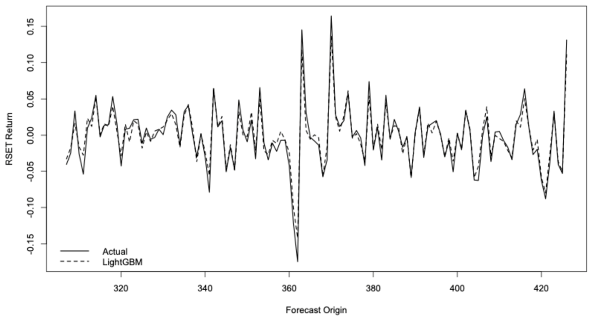
Figure A2.
Actual versus LightGBM Forecast at the 3-Month Horizon.
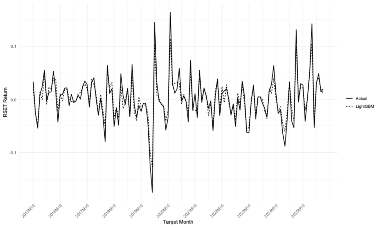
Figure A3.
Actual versus LightGBM Forecast at the 6-Month Horizon.
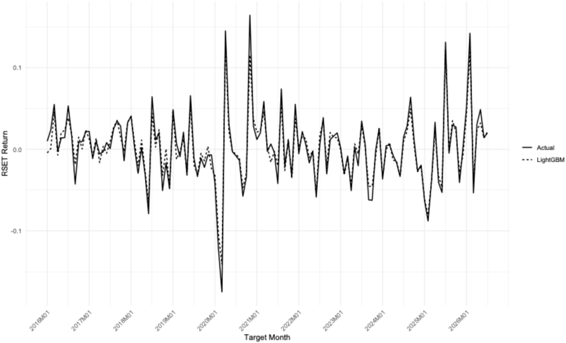
Figure A4.
Actual versus LightGBM Forecast at the 12-Month Horizon.
Appendix B. SHAP-Based Interpretation of the LightGBM Forecast
This appendix provides additional SHAP-based evidence on the predictors underlying the LightGBM forecasts. It complements the summary SHAP results presented in Section 4.1.6 by reporting the predictor set, global feature importance, dependence patterns, and the interpretation of geopolitical risk.
B.1 Purpose of the SHAP Analysis
To improve the interpretability of the LightGBM forecasting model, SHAP (SHapley Additive exPlanations) analysis was employed to examine the contribution of individual predictors to the model's forecasts. Unlike conventional linear models, the tree-based LightGBM framework does not impose a specific linear functional form between the predictors and the forecasted Thai stock-market return. SHAP therefore provides an interpretable decomposition of the model prediction into a baseline component and feature-specific contributions.
The SHAP analysis focuses on identifying which predictors contribute most strongly to the LightGBM forecasts and whether their contributions are associated with positive or negative predicted RSET returns. Mean absolute SHAP values are used to assess the overall importance of each predictor, while SHAP dependence plots are used to examine the relationship between predictor values and their contributions to model predictions.
B.2 Predictor Set
The LightGBM model incorporates twelve lagged values of the Thai stock-market return (RSET), together with geopolitical risk and selected global financial-market variables. The predictor set can be expressed as:
The corresponding forecasting relationship is:
= lagged return of the Stock Exchange of Thailand index
= Geopolitical Risk Index
= Brent crude oil return
= gold return
= U.S. dollar index return
= forecasting error
= nonlinear prediction function estimated by LightGBM
B.3 Global Feature Importance: Complete Numerical Ranking
The global SHAP analysis evaluates the relative importance of predictors according to their average absolute contribution to the LightGBM predictions. A larger mean absolute SHAP value indicates that a predictor contributes more substantially to variation in the model's predicted RSET return. Figure 2 in the main text presents the overall ranking graphically, while Table B1 reports the complete numerical ranking for all 16 predictors.
The global SHAP results identify GPR as the most influential predictor, followed by RSET_l8, RSET_l11, and RSET_l5. The remaining predictors make smaller but non-zero contributions to the LightGBM forecasts. These values represent predictive attribution rather than causal effects.

Table 1.
Global SHAP feature importance of the LightGBM model.
| Rank | Feature | Mean Absolute SHAP |
|---|---|---|
| 1 | GPR | 0.008782704 |
| 2 | RSET_l8 | 0.008160662 |
| 3 | RSET_l11 | 0.006666476 |
| 4 | RSET_l5 | 0.006072976 |
| 5 | RSET_l7 | 0.006071818 |
| 6 | RSET_l4 | 0.005867524 |
| 7 | RGOLD | 0.005496464 |
| 8 | RBRENT | 0.004838127 |
| 9 | RSET_l2 | 0.004774552 |
| 10 | RSET_l3 | 0.004435254 |
| 11 | RSET_l9 | 0.004308624 |
| 12 | RSET_l10 | 0.004247750 |
| 13 | RSET_l6 | 0.003999198 |
| 14 | RSET_l12 | 0.003984996 |
| 15 | RSET_l1 | 0.002816180 |
| 16 | RDXY | 0.002679095 |
B.4 SHAP Dependence Interpretation
SHAP dependence analysis is used to examine how changes in individual predictors are associated with their contribution to the predicted RSET return. The four predictors with the largest mean absolute SHAP values—GPR, RSET_l8, RSET_l11, and RSET_l5—are presented together in Figure 3 in the main text. They are therefore not duplicated in this appendix.
The four dependence plots illustrate nonlinear predictor–contribution patterns in the LightGBM model. Positive SHAP values indicate a contribution toward higher predicted RSET returns, whereas negative SHAP values indicate a contribution toward lower predicted returns. The plots should be interpreted as predictive attribution conditional on the other predictors in the model, not as evidence of causal effects.
B.5 Interpretation of Geopolitical Risk
Particular attention is given to the role of the geopolitical risk index because geopolitical uncertainty constitutes a central variable in the forecasting framework. The inclusion of GPR allows the analysis to examine whether geopolitical conditions contain predictive information for the Thai stock market beyond the historical dynamics of RSET and global financial variables.
The SHAP framework does not imply that a positive or negative SHAP value represents a causal effect of geopolitical risk. Instead, it indicates the direction in which the observed GPR value contributes to the LightGBM prediction conditional on the other predictors included in the model.
This distinction is important because the empirical objective of the forecasting exercise is predictive rather than causal. The model is designed to evaluate whether geopolitical and financial information improves out-of-sample prediction of Thai stock-market returns.
B.6 Interpretation of Nonlinear and Interaction Effects
The use of LightGBM permits nonlinear relationships and interactions among predictors without imposing a predetermined functional form.
Consequently, the SHAP analysis provides information that complements the conventional forecasting results. While RMSE and MAE evaluate how accurately the model forecasts RSET, SHAP analysis provides evidence regarding which information contributes to those forecasts.
This distinction is particularly relevant because the forecasting results indicate that LightGBM performs strongly across the four forecast horizons. LightGBM records the lowest RMSE at the 1- and 12-month horizons, while XGBoost achieves the lowest RMSE at the 3- and 6-month horizons. Thus, the SHAP analysis serves as an interpretability layer for the LightGBM model rather than an additional forecasting-performance test.
B.7 Summary
Overall, the SHAP analysis provides an interpretable representation of the LightGBM forecasting mechanism. The analysis identifies the relative contribution of historical Thai stock-market returns, geopolitical risk, and global financial-market variables to the model's predictions.
The results should be interpreted as predictive contributions rather than causal effects. This interpretation is consistent with the study's primary objective of evaluating the out-of-sample predictive value of geopolitical and financial information for Thai stock-market returns.
The SHAP results therefore complement the RMSE, MAE, Diebold–Mariano, and Model Confidence Set analyses by providing an explanation of the information underlying the forecasts. The forecasting evaluation establishes predictive performance, whereas the SHAP analysis provides model interpretability.
Appendix C. Complete Out-of-Sample Forecast Results
This appendix reports the complete observation-level out-of-sample forecasts underlying the forecast-accuracy results in Table 7. Tables C1–C4 present realized RSET returns together with forecasts from all competing models at each horizon, while Table C5 reports the corresponding Diebold–Mariano comparisons.
Table 1.
Actual and Forecasted RSET Returns: 1-Month-Ahead Horizon.
| Target Month | Actual | ARIMA-GARCH | ARIMAX-GARCH | Random Forest | XGBoost | LightGBM |
|---|---|---|---|---|---|---|
| 2015M08 | -0.040898 | -0.013295 | 0.030512 | -0.023629 | -0.039260 | -0.032576 |
| 2015M09 | -0.024465 | 0.006885 | -0.013415 | -0.006643 | -0.012388 | -0.017205 |
| 2015M10 | 0.033488 | 0.012744 | 0.002147 | 0.021973 | 0.021696 | 0.016289 |
| 2015M11 | -0.025587 | 0.003198 | -0.039067 | -0.007289 | -0.016007 | -0.016008 |
| 2015M12 | -0.054158 | -0.013968 | -0.006959 | -0.027595 | -0.039796 | -0.027386 |
| 2016M01 | 0.010012 | -0.016278 | 0.007901 | 0.013274 | 0.019295 | 0.023413 |
| … | … | … | … | … | … | … |
N = 132 observations Note: Actual denotes the realized monthly RSET return in the target month. Forecasts are generated using an expanding-window out-of-sample forecasting design with a one-month-ahead horizon. ARIMA-GARCH, ARIMAX-GARCH, Random Forest, XGBoost, and LightGBM denote the competing forecasting models. Forecasts are evaluated using the same target observations within each forecasting horizon.
Table 2.
Actual and Forecasted RSET Returns: 3-Month-Ahead Horizon.
| Target Month | Actual | ARIMA-GARCH | ARIMAX-GARCH | Random Forest | XGBoost | LightGBM |
|---|---|---|---|---|---|---|
| 2015M10 | 0.033488 | 0.017396 | 0.005765 | 0.012752 | 0.024046 | 0.019609 |
| 2015M11 | -0.025587 | 0.003762 | -0.026143 | -0.014104 | -0.018764 | -0.025980 |
| 2015M12 | -0.054158 | -0.013326 | -0.021718 | -0.031147 | -0.039094 | -0.048350 |
| 2016M01 | 0.010012 | -0.010740 | 0.009707 | 0.010047 | 0.008782 | 0.013788 |
| 2016M02 | 0.023841 | -0.000985 | 0.036636 | 0.009771 | 0.015918 | 0.000005 |
| 2016M03 | 0.054998 | 0.006479 | 0.034957 | 0.033060 | 0.049329 | 0.048353 |
| … | … | … | … | … | … | … |
N = 130 observations Note: Actual denotes the realized monthly RSET return in the target month. Forecasts are generated using an expanding-window out-of-sample forecasting design with a three-month-ahead horizon. All competing models use the same forecast origins and target observations within this horizon.
Table 3.
Actual and Forecasted RSET Returns: 6-Month-Ahead Horizon.
| Target Month | Actual | ARIMA-GARCH | ARIMAX-GARCH | Random Forest | XGBoost | LightGBM |
|---|---|---|---|---|---|---|
| 2016M01 | 0.010012 | -0.013789 | 0.006298 | 0.000665 | 0.005368 | -0.004325 |
| 2016M02 | 0.023841 | -0.000633 | 0.036708 | 0.008208 | 0.004902 | 0.000876 |
| 2016M03 | 0.054998 | 0.012112 | 0.036703 | 0.029754 | 0.037116 | 0.045860 |
| 2016M04 | -0.002197 | 0.007395 | 0.050891 | -0.005763 | -0.004209 | -0.006982 |
| 2016M05 | 0.013907 | -0.001383 | -0.010679 | 0.010086 | 0.016917 | 0.020413 |
| 2016M06 | 0.014436 | -0.006413 | 0.029071 | 0.019113 | 0.021597 | 0.023485 |
| … | … | … | … | … | … | … |
N = 127 observations Note: Actual denotes the realized monthly RSET return in the target month. Forecasts are generated using an expanding-window out-of-sample forecasting design with a six-month-ahead horizon. All competing models are evaluated over the same set of forecast origins and target observations.
Table 4.
Actual and Forecasted RSET Returns: 12-Month-Ahead Horizon.
| Target Month | Actual | ARIMA-GARCH | ARIMAX-GARCH | Random Forest | XGBoost | LightGBM |
|---|---|---|---|---|---|---|
| 2016M07 | 0.053282 | -0.007506 | -0.002074 | 0.043255 | 0.044777 | 0.048411 |
| 2016M08 | 0.015864 | 0.002883 | 0.002679 | 0.013801 | 0.013563 | 0.023021 |
| 2016M09 | -0.043039 | 0.008713 | 0.002697 | -0.034834 | -0.041470 | -0.054362 |
| 2016M10 | 0.008399 | 0.002445 | -0.022686 | 0.008278 | 0.003517 | 0.014360 |
| 2016M11 | 0.009661 | -0.003645 | -0.014280 | 0.021266 | 0.015689 | 0.033597 |
| 2016M12 | 0.021421 | -0.005134 | 0.018543 | 0.007699 | 0.010376 | 0.014268 |
| … | … | … | … | … | … | … |
N = 121 observations Note: Actual denotes the realized monthly RSET return in the target month. Forecasts are generated using an expanding-window out-of-sample forecasting design with a twelve-month-ahead horizon. All competing models are evaluated over the same set of forecast origins and target observations.
Table 5.
Diebold–Mariano Tests: Best Machine-Learning Model versus ARIMA-GARCH.
| Horizon | Best ML Model | DM (RMSE) | p-value | DM (MAE) | p-value |
|---|---|---|---|---|---|
| 1M | LightGBM | -4.472 | <0.001 | -9.354 | <0.001 |
| 3M | XGBoost | -3.634 | <0.001 | -7.658 | <0.001 |
| 6M | XGBoost | -3.936 | <0.001 | -8.930 | <0.001 |
| 12M | LightGBM | -2.706 | 0.008 | -5.203 | <0.001 |
Note: The Diebold–Mariano test evaluates the null hypothesis of equal predictive accuracy between the best-performing machine-learning model and the ARIMA-GARCH benchmark. The test is conducted using squared-error and absolute-error loss functions. Negative DM statistics indicate lower forecast loss for the machine-learning model relative to the benchmark under the ordering used in the test. p-values below 0.05 indicate statistically significant differences in predictive accuracy.
References
- Vancsura, L.; Tatay, T.; Bareith, T. Navigating AI-driven financial forecasting: A systematic review of current status and critical research gaps. Forecasting 2025, 7(3), 36. [Google Scholar] [CrossRef]
- Naifar, N. Do supply-chain stress and geopolitical risk predict strategic commodity and clean energy market returns? Evidence from explainable machine learning. Forecasting 2026, 8(4), 59. [Google Scholar] [CrossRef]
- Caldara, D.; Iacoviello, M. Measuring geopolitical risk. Am. Econ. Rev. 2022, 112(4), 1194–1225. [Google Scholar] [CrossRef]
- Enescu, A.-G.; Răileanu Szeles, M. Geopolitical risks and global stock market dynamics: A quantile-based approach. Int. J. Financ. Stud. 2026, 14(4), 85. [Google Scholar] [CrossRef]
- Zhang, Y.; Zhang, Y.; Ren, X.; Jin, M. Geopolitical risk exposure and stock returns: Evidence from China. Financ. Res. Lett. 2024, 64, 105479. [Google Scholar] [CrossRef]
- Plakandaras, V.; Gupta, R.; Wong, W.-K. Point and density forecasts of oil returns: The role of geopolitical risks. Resour. Policy 2019, 62, 580–587. [Google Scholar] [CrossRef]
- Schlosky, M. T. T.; Karadas, S.; Stivers, A. Forecasting U.S. stock returns conditional on geopolitical risk and business cycles. Int. Rev. Financ. Anal. 2024, 96(Part B), 103707. [Google Scholar] [CrossRef]
- Rafi, M. K. H.; Ali, S. R. M. Disaggregated geopolitical risks and global stock returns. Glob. Financ. J. 2025, 67, 101151. [Google Scholar] [CrossRef]
- Chopra, R.; Sharma, G. D. Application of artificial intelligence in stock market forecasting: A critique, review, and research agenda. J. Risk Financ. Manag. 2021, 14(11), 526. [Google Scholar] [CrossRef]
- Khan, A. H.; Shah, A.; Ali, A.; Shahid, R.; Zahid, Z. U.; Sharif, M. U.; Jan, T.; Zafar, M. H. A performance comparison of machine learning models for stock market prediction with novel investment strategy. PLoS ONE 2023, 18(9), e0286362. [Google Scholar] [CrossRef]
- Cakici, N.; Zaremba, A. What drives stock returns across countries? Insights from machine learning models. Int. Rev. Financ. Anal. 2024, 96(Part A), 103569. [Google Scholar] [CrossRef]
- Niu, Z.; Wang, C.; Zhang, H. Forecasting stock market volatility with various geopolitical risks categories: New evidence from machine learning models. Int. Rev. Financ. Anal. 2023, 89, 102738. [Google Scholar] [CrossRef]
- Dickey, D. A.; Fuller, W. A. Distribution of the estimators for autoregressive time series with a unit root. J. Am. Stat. Assoc. 1979, 74(366), 427–431. [Google Scholar] [CrossRef]
- Phillips, P. C. B.; Perron, P. Testing for a unit root in time series regression. Biometrika 1988, 75(2), 335–346. [Google Scholar] [CrossRef]
- Kwiatkowski, D.; Phillips, P. C. B.; Schmidt, P.; Shin, Y. Testing the null hypothesis of stationarity against the alternative of a unit root. J. Econom. 1992, 54(1–3), 159–178. [Google Scholar] [CrossRef]
- Box, G. E. P.; Jenkins, G. M.; Reinsel, G. C.; Ljung, G. M. Time series analysis: Forecasting and control, 5th ed.; Wiley, 2015. [Google Scholar]
- Engle, R. F. Autoregressive conditional heteroscedasticity with estimates of the variance of United Kingdom inflation. Econometrica 1982, 50(4), 987–1007. [Google Scholar] [CrossRef]
- Bollerslev, T. Generalized autoregressive conditional heteroskedasticity. J. Econom. 1986, 31(3), 307–327. [Google Scholar] [CrossRef]
- Breiman, L. Random forests. Mach. Learn. 2001, 45(1), 5–32. [Google Scholar] [CrossRef]
- Chen, T.; Guestrin, C. XGBoost: A scalable tree boosting system. In Proceedings of the 22nd ACM SIGKDD. International Conference on Knowledge Discovery and Data Mining; Association for Computing Machinery, 2016; pp. 785–794. [Google Scholar] [CrossRef]
- Ke, G.; Meng, Q.; Finley, T.; Wang, T.; Chen, W.; Ma, W.; Ye, Q.; Liu, T.-Y. LightGBM: A highly efficient gradient boosting decision tree. Adv. Neural Inf. Process. Syst. 2017, 30, 3146–3154. [Google Scholar]
- Hyndman, R. J.; Athanasopoulos, G. Forecasting: Principles and practice, 3rd ed.; OTexts, 2021; Available online: https://otexts.com/fpp3/23.
- Diebold, F.X.; Mariano, R.S. Comparing Predictive Accuracy. J. Bus. Econ. Stat. 1995, 13(3), 253–263. [Google Scholar] [CrossRef]
- Hansen, P.R.; Lunde, A.; Nason, J.M. The Model Confidence Set. Econometrica 2011, 79(2), 453–497. [Google Scholar] [CrossRef]
- Lundberg, S. M.; Lee, S.-I. A unified approach to interpreting model predictions. Adv. Neural Inf. Process. Syst. 2017, 30, 4765–4774. [Google Scholar]
- Gupta, R.; Karmakar, S.; Pierdzioch, C. Safe havens, machine learning, and the sources of geopolitical risk: A forecasting analysis using over a century of data. Comput. Econ. 2024, 64, 487–513. [Google Scholar] [CrossRef]
Figure 1.
Residual diagnostics for the ARIMA–GARCH(1,1) benchmark model.
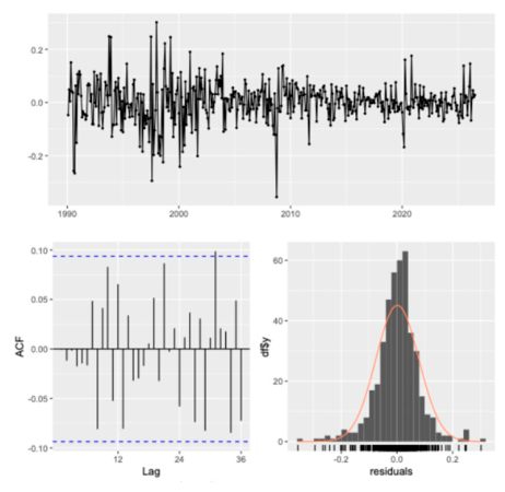
Table 1.
Definition and Use of Variables.
| Variable | Definition / Construction | Role |
|---|---|---|
| Dependent variable | ||
| Geopolitical Risk Index | External predictor | |
| External predictor | ||
| External predictor | ||
| External predictor | ||
| ML predictors |
Note: GPR is used in its original index form, whereas price-based financial variables are transformed into continuously compounded returns. The machine-learning models use the first 12 lags of RSET together with GPR, RBRENT, RGOLD, and RDXY.
Table 2.
Descriptive Statistics.
| Variable | Mean | Median | SD | Min | Max | Skewness | Kurtosis | JB | N |
|---|---|---|---|---|---|---|---|---|---|
| RSET | 0.0015 | 0.0056 | 0.0785 | −0.3592 | 0.2843 | −0.3233 | 6.0321 | 175.41 | 439 |
| GPR | 104.8863 | 92.0200 | 52.0969 | 39.0500 | 512.5300 | 3.6615 | 23.0016 | 8,298.74 | 439 |
| RBRENT | 0.0034 | 0.0063 | 0.0988 | −0.6339 | 0.3796 | −0.5823 | 8.3467 | 546.47 | 439 |
| RGOLD | 0.0052 | 0.0012 | 0.0448 | −0.2041 | 0.1519 | −0.1292 | 4.1872 | 26.94 | 439 |
| RDXY | 0.0002 | −0.0007 | 0.0230 | −0.0651 | 0.0975 | 0.3273 | 3.8190 | 20.06 | 439 |
Note: JB denotes the Jarque–Bera normality statistic. The null hypothesis of normality is rejected for all variables at the 1% significance level.
Table 3.
Unit Root Test Results.
| Variable | ADF p-value | PP p-value | KPSS p-value | Conclusion |
|---|---|---|---|---|
| RSET | <0.01 | <0.01 | >0.10 | I(0) |
| GPR | <0.01 | <0.01 | >0.10 | I(0) |
| RBRENT | <0.01 | <0.01 | >0.10 | I(0) |
| RGOLD | <0.01 | <0.01 | 0.0446 | I(0)* |
| RDXY | <0.01 | <0.01 | >0.10 | I(0) |
Note: * The KPSS test rejects level stationarity at the 5% level; however, the ADF and PP tests both reject the unit-root null at the 1% level.
Table 4.
Out-of-sample forecasting design.
| Element | Specification |
|---|---|
| Full sample | Jan 1990 – Jul 2026 |
| Observations | 439 |
| Initial training window | Jan 1990 – Jul 2015 (307 observations) |
| Forecasting scheme | Expanding-window rolling-origin |
| First forecast origin | Jul 2015 |
| First forecast target | Aug 2015 |
| Forecast horizons | 1-, 3-, 6-, and 12-month ahead |
| Evaluation endpoint | Jul 2026 |
| Information constraint | No future/contemporaneous information |
| External predictors | Lagged GPR, RBRENT, RGOLD, RDXY |
| Accuracy measures | RMSE, MAE |
| Pairwise comparison | Diebold–Mariano test |
| Multiple-model comparison | Model Confidence Set |
Note: All competing models are evaluated using the same forecasting procedure and information constraints within each forecast horizon.
Table 5.
Estimation and diagnostic results for the ARIMA–GARCH benchmark model.
| Component | Parameter/Test | Estimate/Statistic | p-value |
|---|---|---|---|
| Mean equation | AR(1) | 0.899 | <0.001 |
| AR(2) | −1.022 | <0.001 | |
| AR(3) | 0.076 | 0.020 | |
| MA(1) | −0.837 | <0.001 | |
| MA(2) | 0.989 | <0.001 | |
| Variance equation | ω | 0.000115 | 0.139 |
| α₁ | 0.151 | 0.008 | |
| β₁ | 0.837 | <0.001 | |
| α₁ + β₁ | 0.988 | — | |
| Distribution | Student-t shape | 6.352 | <0.001 |
| Diagnostics | Ljung–Box, standardized residuals | 11.878 | 0.567 |
| Ljung–Box, squared standardized residuals | 4.005 | 0.588 | |
| ARCH LM, lag 7 | 2.724 | 0.567 | |
| Nyblom joint stability | 1.853 | — | |
| Sign-bias joint test | 2.731 | 0.435 |
Note: Robust standard errors are used for parameter inference. Diagnostic tests are based on standardized residuals. Volatility persistence is measured as α₁ + β₁.
Table 6.
Estimation and diagnostic results for the ARIMAX–GARCH benchmark model.
| Component | Parameter/Test | Estimate/Statistic | p-value |
|---|---|---|---|
| Mean equation | AR(1) | 0.924 | <0.001 |
| AR(2) | −0.882 | <0.001 | |
| MA(1) | −0.907 | <0.001 | |
| MA(2) | 0.930 | <0.001 | |
| GPRₜ₋₁ | 0.000105 | 0.052 | |
| RBRENTₜ₋₁ | −0.0719 | 0.029 | |
| RGOLDₜ₋₁ | 0.0300 | 0.711 | |
| RDXYₜ₋₁ | −0.2021 | 0.162 | |
| Variance equation | ω | 0.000121 | 0.138 |
| α₁ | 0.140 | 0.011 | |
| β₁ | 0.844 | <0.001 | |
| α₁ + β₁ | 0.984 | — | |
| Distribution | Student-t shape | 6.076 | <0.001 |
| Diagnostics | Ljung–Box, standardized residuals | 8.780 | 0.675 |
| Ljung–Box, squared standardized residuals | 4.076 | 0.576 | |
| ARCH LM, lag 7 | 2.874 | 0.538 | |
| Nyblom joint stability | 3.150 | — | |
| Sign-bias joint test | 2.081 | 0.556 |
Note: Robust standard errors are used for parameter inference. Diagnostic tests are based on standardized residuals. Volatility persistence is measured as α₁ + β₁.
Table 7.
Out-of-Sample Forecasting Performance of Competing Models.
| Forecast horizon | Model | RMSE | MAE | N |
|---|---|---|---|---|
| 1-month | ARIMA-GARCH | 0.0462 | 0.0322 | 132 |
| ARIMAX-GARCH | 0.0431 | 0.0317 | 132 | |
| Random Forest | 0.0197 | 0.0136 | 132 | |
| XGBoost | 0.0132 | 0.0101 | 132 | |
| LightGBM | 0.0107 | 0.0081 | 132 | |
| 3-month | ARIMA-GARCH | 0.0468 | 0.0339 | 130 |
| ARIMAX-GARCH | 0.0425 | 0.0312 | 130 | |
| Random Forest | 0.0197 | 0.0139 | 130 | |
| XGBoost | 0.0113 | 0.0088 | 130 | |
| LightGBM | 0.0146 | 0.0110 | 130 | |
| 6-month | ARIMA-GARCH | 0.0476 | 0.0337 | 127 |
| ARIMAX-GARCH | 0.0434 | 0.0318 | 127 | |
| Random Forest | 0.0195 | 0.0133 | 127 | |
| XGBoost | 0.0110 | 0.0083 | 127 | |
| LightGBM | 0.0111 | 0.0084 | 127 | |
| 12-month | ARIMA-GARCH | 0.0469 | 0.0331 | 121 |
| ARIMAX-GARCH | 0.0446 | 0.0326 | 121 | |
| Random Forest | 0.0205 | 0.0139 | 121 | |
| XGBoost | 0.0119 | 0.0088 | 121 | |
| LightGBM | 0.0103 | 0.0080 | 121 |
Note: RMSE and MAE are calculated from the complete observation-level out-of-sample forecasts. Lower values indicate better forecasting performance. Bold values indicate the lowest error among competing models within each forecasting horizon. The number of observations varies across horizons because longer-horizon forecasts reduce the number of available forecast origins. The complete observation-level actual and forecasted values underlying these accuracy measures are reported in Appendix C (Tables C1–C4).
Table 8.
Diebold–Mariano Tests of Predictive Accuracy.
| Comparison | h=1 DM (p) | h=3 DM (p) | h=6 DM (p) | h=12 DM (p) |
|---|---|---|---|---|
| LightGBM vs ARIMA-GARCH | −4.054 (<0.001) | −3.331 (0.001) | −3.502 (<0.001) | −2.654 (0.009) |
| LightGBM vs ARIMAX-GARCH | −4.434 (<0.001) | −3.360 (0.001) | −3.189 (0.002) | −2.689 (0.008) |
| LightGBM vs Random Forest | −3.755 (<0.001) | −2.480 (0.015) | −2.310 (0.023) | −2.196 (0.030) |
| LightGBM vs XGBoost | −3.435 (<0.001) | −1.277 (0.204) | −0.032 (0.974) | −1.031 (0.305) |
Table 9.
Model Confidence Set across Forecasting Horizons.
| Model | h=1 | h=3 | h=6 | h=12 |
|---|---|---|---|---|
| ARIMA-GARCH | Eliminated | Eliminated | Eliminated | Eliminated |
| ARIMAX-GARCH | Eliminated | Eliminated | Eliminated | Eliminated |
| Random Forest | Eliminated | Eliminated | Eliminated | Eliminated |
| XGBoost | Eliminated | Retained | Retained | Retained |
| LightGBM | Retained | Retained | Retained | Retained |
Table 10.
Robustness Test: With and Without GPR.
| Forecast horizon | LightGBM | LightGBM without GPR | RMSE change (%) |
|---|---|---|---|
| 1-month | 0.01060 | 0.01124 | 5.71 |
| 3-month | 0.01029 | 0.01115 | 7.69 |
| 6-month | 0.01098 | 0.01097 | −0.12 |
| 12-month | 0.01035 | 0.00964 | −7.43 |
Note: Positive values indicate lower RMSE for the full LightGBM specification relative to the model without GPR. RMSE changes are calculated using unrounded RMSE values; displayed RMSE values are rounded to five decimal places.
Disclaimer/Publisher’s Note: The statements, opinions and data contained in all publications are solely those of the individual author(s) and contributor(s) and not of MDPI and/or the editor(s). MDPI and/or the editor(s) disclaim responsibility for any injury to people or property resulting from any ideas, methods, instructions or products referred to in the content. |
© 2026 by the authors. Licensee MDPI, Basel, Switzerland. This article is an open access article distributed under the terms and conditions of the Creative Commons Attribution (CC BY) license (http://creativecommons.org/licenses/by/4.0/).
Copyright: This open access article is published under a Creative Commons CC BY 4.0 license, which permit the free download, distribution, and reuse, provided that the author and preprint are cited in any reuse.