

Submitted:
19 August 2026
Posted:
20 August 2026
You are already at the latest version
Abstract
We propose a reinforcement learning framework in which exploration is driven by intrinsic curiosity,designed for scenarios where environments are non-stationary and rewards are sparse, delayed, unin-formative, or absent. In our model, action selection is guided by a combination of external rewardsand an epistemic motivation mechanism that biases the agent toward structured exploratory directions.The central hypothesis is that effective exploration emerges at intermediate levels of incoherence, whileperformance degrades under both overly rigid and overly disordered dynamics. To test this idea, weimplement the framework on top of a Liquid State Machine (LSM) substrate and evaluate it on twostandard benchmarks—the discrete-action LunarLander-v2 and the continuous-control BipedalWalker-v3. The proposed method achieves competitive performance on both tasks relative to established deepRL algorithms, including Proximal Policy Optimization (PPO) and Intrinsic Curiosity Module (ICM).We further show that the curiosity window is not recovered in Active Inference agents under the sameanalysis, suggesting that the proposed dynamics capture a distinct exploration regime.
Keywords:
curiosity window
; liquid state machines
; active inference
; intrinsic motivation
; reservoir computing
; exploration–exploitation
1. Introduction
The problem of exploration in adaptive systems—how an agent discovers useful behaviours without exhaustive search—remains central to reinforcement learning (RL), cognitive science, and theories of consciousness. Standard approaches treat exploration as an external mechanism: -greedy schedules, Boltzmann temperature annealing, count-based bonuses, or prediction-error curiosity signals (Burda et al. 2018; Pathak et al. 2017). In each case, the drive to explore is designed in rather than emerging from the system’s own dynamics.
Despite significant progress, most modern approaches still rely on exogenous mechanisms such as -greedy noise, entropy regularisation, or intrinsic reward proxies based on prediction error or state novelty. While these methods improve exploration in specific settings, they do not provide a general solution: they require careful tuning, often fail under non-stationarity, and tend to collapse either into premature exploitation or unstructured random behaviour. More recent advances—including Soft Actor-Critic (SAC), Twin Delayed DDPG (TD3), and curiosity-driven methods such as ICM (Pathak
38 et al. 2017) and RND (Burda et al. 2018)—improve stability and performance but still treat exploration as an auxiliary objective rather than as an endogenous consequence of the agent’s internal dynamics. Consequently, they struggle in regimes where reward is sparse, absent, or shifting, and they lack a principled account of when exploration should increase or decrease. This gap suggests that the core issue is conceptual: current frameworks do not capture the conditions under which meaningful, structured exploration should emerge.
We propose a different approach. Instead of optimising a single external objective, we posit that systems self-regulate coherently between functionally differentiated fields. Exploration arises endogenously when incoherence reaches an intermediate regime—neither so low that the system is trapped, nor so high that it fragments. This prediction, termed the Curiosity Window conjecture, is the framework’s most distinctive and testable claim.
In this paper, we provide the first computational validation of these ideas, implemented through a Liquid State Machine (LSM) substrate. We demonstrate that systems self-organise around a curiosity window, compare our agents against Active Inference (AIF) baselines, and test whether endogenous noise modulation can sustain exploration without external signals. Our contributions are:
- 1.
- Curiosity Window: The metric (coherent basins × global overlap × transition rate) peaks at intermediate noise, with drop-off on both sides (Section 4).
- 2.
- Endogenous exploration: The curiosity window is specific to our model—AIF agents show no analogous peak (Section 5.3).
- 3.
- Extended dynamics: Spatial coupling, sedimentation learning, and non-stationary adaptation are validated (Section 5.4).
2. Summary of the Coherence Framework
We posit that experience is not a passive reception of data but an active regulation of coherence between what is open (possible continuations) and what is constrained (current situational demands). Unlike the Free Energy Principle (FEP), which derives behaviour from surprise minimisation over generative models, we treat coherence regulation as primitive and representational structures as secondary invariances that may or may not emerge.
Three principles govern the framework:
- 1.
- Coherence Primacy: The primitive explanatory target is the regulation of coherence between reach and yield. Representational structures are secondary.
- 2.
- Functional Differentiation: Openness and constraint must be functionally differentiated; undifferentiated dynamics cannot express the framework’s characteristic tension.
- 3.
- Mutual Constraint: Reach must be constrained by yield, yield must matter for reach, and memory must affect the trajectory of both.
2.1. Mathematical Setting
Let denote the experiential field, a measurable space equipped with a -algebra and a reference measure . Three time-dependent densities are defined on :
Definition 1
(Functional Roles).
- Reach: the distribution over viable continuations (openness, action tendency).
- Yield: the distribution reflecting current environmental and internal constraint.
- Memory: the sedimented trace of past coherence achievements.
Two functionals measure the system’s coherence state:
Definition 2
(Incoherence).
Definition 3
(Global Overlap).
The global overlap is the Bhattacharyya coefficient between reach and yield; it equals 1 when and approaches 0 when the two distributions have disjoint support. In the discrete implementations that follow, the integral is replaced by a finite sum over field cells.
The dynamics are governed by coupled update rules:
where are learning rates, maps reservoir state and input to yield, is the noise scale, and is i.i.d. noise.
Conjecture 1
(Curiosity Window). There exists an intermediate regime of incoherence such that a suitable curiosity metric is maximised. Below , the system is trapped in coherent but unexplorative basins; above , the system fragments and loses coherent structure.
The Curiosity Window proof (Appendix A) relies on a curiosity functional whose specific form—coherent basin occupancy times global overlap times transition rate—was introduced computationally. The key insight is that incoherence , measuring reach–yield tension, and global overlap , measuring system-level alignment (Definitions 2 and 3), together capture the essential ingredients of curiosity: the endogenous opening of new viable possibilities driven by unresolved internal tension. This requires:
- 1.
- that the system visits distinct coherent configurations (not merely fluctuates randomly);
- 2.
- that it does so while maintaining global integration (not fragmenting);
- 3.
- that the exploration is structured—transitions between identifiable basins, not diffusion through undifferentiated state space.
2.2. Representation Theorem
Theorem 1
(Representation of the curiosity functional). Let be a curiosity functional of the form where F is continuous and separately monotone in each argument (increasing in G, , and ). Then:
- 1.
- F vanishes on the boundary: for all values of the remaining arguments below their respective thresholds.
- 2.
- F is uniquely determined up to monotone transformation by the product form: there exists a strictly increasing with such that
Proof is presented in Appendix B.
2.3. Sedimentation as Learning
We treat learning not as parameter updates to a loss function but as sedimentation: the progressive shaping of the memory field through repeated coherence episodes. States that have repeatedly achieved low incoherence acquire higher probability mass in the baseline reach , making future coherence in those regions easier. This is formalised as:
where is the sedimentation rate and are recency weights.
3. Computational Architecture and Implementation
Our computational realisation is structured as a two-layer architecture: (i) a dynamical substrate providing high-dimensional temporal representations, and (ii) a coherence-regulating control layer implementing the field dynamics.
The substrate is instantiated as a Liquid State Machine (LSM), while the coherence layer defines the evolution of the reach (), yield (y), and memory (m) fields, together with the endogenous modulation of exploration. This separation is essential: the LSM supplies a rich, fading-memory embedding of experience, whereas the coherence layer provides the governing principles of organisation and exploration.
3.1. Liquid State Machine Substrate
We model the experiential field as the state space induced by a recurrent reservoir. The reservoir state evolves according to:
where is a sparse recurrent weight matrix with spectral radius , maps sensory input into the reservoir, and represents intrinsic perturbations.
The LSM provides:
- high-dimensional nonlinear expansion of inputs,
- fading memory of past states,
- continuous-time-like dynamics suitable for temporal integration.
Crucially, the reservoir itself is not the agent: it serves as a dynamical medium over which the coherence variables are defined and updated.
3.2. State Augmentation and Temporal Thickness
To capture temporal extension explicitly, we augment the instantaneous reservoir state with a slow trace:
and define the effective substrate representation as:
This construction provides both fast dynamics (x) and sedimented temporal structure (h), aligning the implementation with the requirement of temporally extended coherence.
3.3. Field Representation and Extraction
The fields are defined as probability distributions over a discretised version of the reservoir state space. Given , we construct:
where is typically the identity or a linear projection, and are learned or fixed mappings.
The three fields play distinct roles:
- : reach (action tendency / exploratory distribution),
- : yield (constraint induced by environment and internal state),
- : memory (sedimented trace of past coherent states).
3.4. Field Dynamics
The coupled dynamics of the fields follow:
These equations implement:
- Mutual constraint: reach is shaped by yield, and yield depends on reach,
- Temporal integration: memory accumulates past reach states,
- Non-equilibrium dynamics: the system continuously reconfigures rather than converging to a static optimum.
The variable m should not be interpreted as memory in the classical RL sense (e.g., a replay buffer or explicit storage of past transitions). Instead, m represents a sedimented internal trace: a continuously updated latent summary of the agent’s recent and recurrent interactions with the environment. It evolves as a slow-moving average of the reach distribution , capturing what has become statistically stable for the agent over time. Deviations between and signal novelty or drift, while alignment indicates coherence and stability. In this sense, m functions as a dynamic baseline of “what is normal,” enabling regulation of exploration without requiring episodic recall.
3.5. Endogenous Exploration Mechanism
A central feature of the architecture is the replacement of exogenous noise with endogenous modulation:
where
This function is unimodal in I, ensuring:
- low noise under high coherence (exploitation),
- low noise under extreme incoherence (fragmentation),
- maximal exploration at intermediate incoherence (curiosity window).
This mechanism closes the loop between internal state and exploration, making curiosity an emergent property rather than an externally imposed signal.
3.6. Spatial Structure and Basin Dynamics
The discretised field is partitioned into K basins representing metastable regions of coherent organisation. Basin assignment at time t is determined by dominant probability mass:
To enforce global integration, a spatial coupling kernel can be applied:
This allows local perturbations to propagate across the field, preventing fragmentation and supporting coherent large-scale dynamics.
The complete system can be summarised as:
- LSM substrate: provides high-dimensional, temporally rich state representation,
- Coherence fields: encode openness (), constraint (y), and memory (m),
- Coupled dynamics: enforce mutual constraint and temporal integration,
- Endogenous noise: links incoherence to exploration intensity,
- Sedimentation: implements learning as structural bias.
This architecture differs fundamentally from standard RL systems: exploration is not injected but generated by the system’s own coherence dynamics, yielding a closed-loop, self-regulating process.
4. The Curiosity Window
The notion of a curiosity window arises from a central limitation in existing exploration strategies: they lack a principled account of when exploration should occur. In most RL frameworks, exploration is either externally imposed (e.g., fixed noise, entropy bonuses) or monotonically controlled, leading to two well-known failure modes: premature convergence or unstructured randomness.
Our framework predicts that effective exploration self-organises within a bounded intermediate regime. When incoherence is too low, the system becomes overly stable and is trapped in a limited set of behaviours. When incoherence is too high, structure is lost and exploration becomes fragmented and unproductive. Between these extremes lies the curiosity window: a regime in which the system explores multiple possibilities while maintaining enough internal coherence to make that exploration meaningful.
Definition 4
(Curiosity functional ). Let be a trajectory of the coherence dynamic on with basin partition . Thecuriosity functionalis
The three factors of correspond to three distinct commitments:
- : Global overlap. Ensures that the field remains unified. Without G, a fragmented system that randomly visits many regions would score high on curiosity—violating the requirement that curiosity occurs within a coherent field.
- : Coherent basin count. Ensures that the system has differentiated metastable structure. A system with only one basin cannot exhibit the structured transitions needed for learning and creativity.
- : Transition rate. Ensures that the system is actively moving between basins, not merely possessing the potential to do so. This is the dynamical signature of intrinsic curiosity: the system reorganises because internal tension drives it to explore.
The curiosity functional is not an ad hoc choice. By Theorem 1, it is the unique (up to monotone transformation) continuous, separately monotone, dimensionally consistent functional of the three quantities—global overlap, coherent basin count, and inter-basin transition rate—that satisfies the boundary conditions derived from the framework’s foundational commitments. Any system that scores high on is simultaneously integrated (G high), differentiated (), and dynamically reorganising ()—precisely the conditions identified with intrinsic curiosity.
5. Toy Experiments
To evaluate the Curiosity Window conjecture under controlled conditions, we implemented the two-layer architecture (LSM substrate + coherence field dynamics) described in Section 3. The reach noise parameter serves as the main control variable.
Environment.
The field evolves in a structured landscape defined by five Gaussian basins at fixed positions in a 40-cell space. These basins create a multi-attractor surface against which the dynamics of exploration and trapping can be measured. The sensory input to the LSM is a 5-dimensional signal derived from the current field state plus additive noise.
5.1. Simulation 1: Phase-Diagram Sweep
The first experiment tests whether curiosity is maximised at an intermediate level of incoherence. We swept the reach-noise parameter in the range
using 45 logarithmically spaced values, while fixing the field-coupling strength at . Each run lasted time steps.
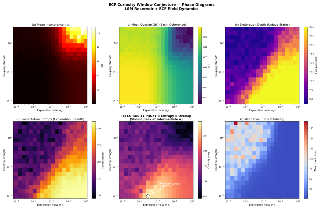
For each run we measured: mean incoherence , mean global overlap , the exploration entropy over the macro-basin visitation histogram, the mean dwell time within a basin before transition, the number of coherent basins (defined as basins with dwell time steps), and the basin transition rate.
Figure 1.
Phase diagram of exploration dynamics across noise regimes. Each panel shows a different property of the dynamics as a function of the reach-noise parameter : mean incoherence , global overlap , basin coherence, exploration entropy, dwell time, transition rate, and composite curiosity metrics. The curiosity window (bottom centre) is visible as a distinct intermediate regime.
Figure 1.
Phase diagram of exploration dynamics across noise regimes. Each panel shows a different property of the dynamics as a function of the reach-noise parameter : mean incoherence , global overlap , basin coherence, exploration entropy, dwell time, transition rate, and composite curiosity metrics. The curiosity window (bottom centre) is visible as a distinct intermediate regime.
5.2. Simulation 2: Three-Regime Time Series
To visualise the dynamics underlying the phase diagram, we selected three representative noise values and ran full 1500-step trajectories (Figure 2):
- Low noise (trapped regime): reach collapses onto one or two basins; overlap remains high, incoherence remains low, and exploration entropy is near zero.
- Intermediate noise (curious regime): the system visits multiple basins with sustained dwell times while maintaining moderate-to-high overlap. This regime operationalises the Curiosity Window.
- High noise (fragmented regime): the system rapidly switches across basins without sustained occupancy; entropy is high but overlap collapses because reach and yield decouple.
A clear three-regime structure emerges. At low noise, the system exhibits overcoherent trapping: low incoherence, high overlap, long dwell times, and minimal exploration. At high noise, the system enters a fragmented regime: high incoherence, collapsed overlap, frequent transitions, and loss of basin structure.
Between these extremes lies the intermediate regime in which structured exploration is maximised. The system maintains moderate incoherence while preserving significant global overlap, visiting multiple basins with sustained occupancy. This balance is captured by , which exhibits a clear interior peak.
Importantly, exploration quality is not monotonic with noise: while entropy increases steadily, only the combination of exploration and coherence yields effective behaviour. This highlights the necessity of intermediate incoherence for intrinsically motivated exploration.
Interpretive criterion.
The core prediction is not simply that entropy should increase with noise, but that coherent exploration should peak at an intermediate noise level. In the simulations, incoherence increased monotonically with , while overlap decreased monotonically, as expected. The non-trivial result is that the product of exploration and coherence peaks only when curiosity is defined structurally rather than purely entropically.
The metric exhibited a distinct interior maximum with a window width of approximately decades in log-space and clear drop-off on both sides.
At low noise (), the system is trapped in a single basin with high overlap but no exploration. At high noise (), the system visits all basins but with fragmented, incoherent transitions. Only at intermediate noise does the system achieve coherent multi-basin exploration—the signature of the curiosity window (Figure 3).
5.3. Endogenous Exploration
A critical test is whether exploration persists when external noise is removed. In the original model with constant , setting at time causes exploration to collapse to of the pre-cutoff rate—a fundamental failure.
Replacing constant noise with the endogenous modulation (Equation 17) creates a self-sustaining feedback loop:
- 1.
- High coherence → low I→ low noise → exploitation.
- 2.
- Exploitation → environment shifts → rising I.
- 3.
- Rising I→ increases → more exploration.
- 4.
- Exploration → new coherence →I decreases.
5.4. Extended Dynamics
Spatial coupling and global integration.
To test global integration, we introduced the spatial coupling kernel (Equation 20). Local perturbation experiments confirmed that disturbances propagate across the full field within 5–10 timesteps in the coupled system, while remaining localised in the uncoupled control.
Sedimentation learning.
We tested whether the memory field accumulates useful structure across episodes. An agent with sedimentation () was compared against a memoryless control across 50 episodes of basin-finding. The sedimented agent showed faster convergence to low-incoherence states and higher final coherence (G), confirming that sedimentation functions as a learning mechanism (Figure 4).
Non-stationary environments.
Basin locations were shifted at to test adaptation. The endogenous model recovered fastest due to the automatic increase in exploration triggered by rising incoherence.
5.5. Sedimentation as Structural Learning
Standard machine learning encodes experience as discrete weight updates via backpropagation. Our framework proposes a fundamentally different mechanism: sedimentation, in which the memory layer accumulates a continuous, coherence-weighted trace of the system’s history. Rather than storing facts, sedimentation deforms the probability landscape itself, biasing future coherence-seeking toward previously successful regions.
5.5.1. Setup
The simulation runs for 60 episodes over a five-basin environment. Each episode presents a different basin as the primary attractor, cycling through Basin 0, Basin 1, and Basin 2 in sequence, so that the relevance of each region shifts over time. Two agents are compared:
- Memory agent—sedimentation active, with the update rulewhere is the global overlap and is the sedimentation rate. High-coherence moments therefore contribute disproportionately to the accumulated trace.
- Control agent—identical architecture with sedimentation disabled (), providing a matched baseline.
5.5.2. Memory Reshapes the Probability Landscape
Over the 60-episode run, the memory distribution undergoes measurable structural change. Shannon entropy of m drops by nats, and the top 10 field positions accumulate of total probability mass (compared with under a uniform distribution). The memory heatmap reveals clear ridges at basin locations: the landscape sculpts itself around coherent regions, concentrating future attractor pull where the system has previously achieved high G.
5.5.3. Sedimentation Tracks Environmental Relevance
The episode schedule shifts emphasis progressively from Basin 0 to Basin 1 to Basin 2. Memory follows this shift with a measurable lag. At the end of training, Basin 2 holds the largest mass (), Basin 1 the next (), and Basin 0 the least (). Crucially, the system does not merely accumulate—it forgets what is no longer relevant. Because older sedimentation fades through the exponential moving average in Equation (22), new coherence patterns progressively overwrite stale ones.
5.5.4. Sedimentation Confers a Measurable Learning Advantage
Table 1 reports the quantitative comparison between the memory and control agents.
The memory agent achieves higher coherence faster because sedimented regions exert an additional pull on , drawing the field toward previously successful attractor configurations. The percentage-point advantage in incoherence reduction compounds across episodes: each high-coherence moment makes the next one slightly easier to reach.
5.5.5. How Sedimentation Differs from Neural Network Learning
Four structural differences distinguish sedimentation from standard gradient-based learning:
- 1.
- No weight updates. The system’s “parameters” form a continuous probability landscape, not a vector of discrete weights. Learning is a smooth, ongoing deformation of this landscape. There is no loss function and no optimisation objective.
- 2.
- Coherence-gated storage. Only high-coherence moments contribute strongly to , because the update is weighted by (Equation (22)). Low-coherence episodes barely register. This is structurally closer to how emotional salience gates consolidation in biological memory than to how backpropagation treats all training examples equally.
- 3.
- Structural forgetting without catastrophe. Old patterns fade naturally through the exponential decay term . There is no catastrophic forgetting, but equally no permanent storage. Stability and plasticity are balanced by a single parameter .
- 4.
- Memory drives exploration. The memory-gradient term in the update pushes the field away from over-sedimented regions, so consolidation does not collapse the system into a fixed attractor. Learning simultaneously consolidates successful patterns and opens new territory.
5.6. Multi-Room Gridworld with Shifting Rewards
We used a custom gridworld partitioned into four rooms with centres at , , , and . The agent started at the centre of the grid and received reward proportional to its proximity to the currently active room centre. The active reward room shifted every 200 steps, cycling through all four rooms. This non-stationarity penalises agents that exploit a single learned policy and rewards those capable of sustained re-exploration.
The ECF agent was compared against a standard -greedy Q-learning baseline. Both agents used identical Q-tables and learning rates (, ). The key difference was the exploration mechanism: the baseline decayed from 0.3 toward 0.01 on a fixed schedule, while the ECF agent modulated exploration endogenously via . When the reward room shifted, the ECF agent’s incoherence spiked as its reach distribution diverged from the now-misaligned yield y, automatically increasing exploration noise. When the agent settled into the new reward region, incoherence dropped and exploitation resumed.
The ECF agent adapted more rapidly to reward shifts. After each transition, its recovery time—measured as the number of steps to return to of peak reward rate—was consistently shorter than the baseline’s. The sedimentation mechanism also contributed: after visiting all four rooms, the memory field m developed peaks at each room centre, biasing future exploration toward previously productive regions.
This experiment established the basic viability of ECF-augmented RL but was limited by the simplicity of the environment. The next experiments were designed to test the framework in more challenging settings.
6. Reinforcement Learning Experiments
To evaluate whether coherence-seeking dynamics confer practical advantages in RL settings, we conducted progressively more demanding experiments. Each experiment stress-tests a specific claim: that endogenous curiosity driven by incoherence produces more adaptive exploration than standard strategies, that this advantage grows under non-stationary conditions, and that the mechanism generalises from discrete to continuous action spaces. In all experiments, the ECF agent maintained full field dynamics—reach (), yield (y), and memory (m) distributions over basins—with incoherence , global overlap , and the endogenous noise function , where peaks at intermediate incoherence .
6.1. ECF–PPO Hybrid Approach
To address more complex RL problems we implemented a hybrid approach (ECF–PPO) combining the optimisation stability of Proximal Policy Optimization (PPO) with an auxiliary memory-based dynamical system. PPO provides the RL backbone through a policy network and a value function , while the ECF module augments the agent with internal latent variables that track current experience, expectation, and memory.
Let denote a latent encoding of the observation . The ECF module maintains three internal quantities: a policy-side expectation , a current experience signal , and a sedimented memory trace . The dynamics are:
with richer variants replacing the single memory trace by multi-timescale components (fast, medium, and slow). From these variables we define an incoherence signal and a novelty signal:
These quantities are transformed into an intrinsic drive , gated by a coherence factor and a controller :
PPO’s role is unchanged at the optimisation level: it performs policy and value updates with clipped objectives and advantage estimation. The difference is that the reward stream now contains a structured intrinsic component derived from internal consistency, novelty, and memory mismatch.
Figure 5.
Architecture of the ECF–PPO hybrid agent. The LSM substrate produces a latent encoding , from which the ECF module computes reach (), yield (), and memory () fields. Incoherence and novelty signals modulate an intrinsic reward that augments the external reward before PPO updates the policy.
Figure 5.
Architecture of the ECF–PPO hybrid agent. The LSM substrate produces a latent encoding , from which the ECF module computes reach (), yield (), and memory () fields. Incoherence and novelty signals modulate an intrinsic reward that augments the external reward before PPO updates the policy.
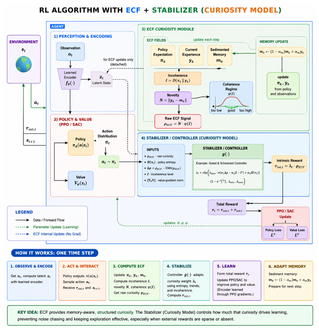
PPO contributes stable policy optimisation and strong baseline performance, while the ECF module contributes internal structure: tracking what is familiar, what is changing, and what is inconsistent with the agent’s latent expectations. The resulting agent is guided by a memory-conditioned internal signal that favours structured exploration over purely random behaviour.
6.2. LunarLander-v2 Stress Test
We used the OpenAI Gymnasium LunarLander-v2 environment, which requires the agent to control a spacecraft’s thrusters to land safely on a pad. The eight-dimensional continuous state space (position, velocity, angle, angular velocity, leg contact) was discretised into bins for tabular Q-learning.
6.2.1. ECF-RichMem Algorithm
To handle this more complex problem we developed an extended version of ECF: ECF-RichMem. It extends the basic formulation by incorporating a multi-timescale memory structure that captures both short-term fluctuations and long-term regularities.
Let denote the environment state at time t, and let be a latent encoding. The agent maintains three internal variables:
- : current experiential state,
- : endogenous expectation (policy-side latent),
- : multi-timescale memory (fast, medium, slow components).
Internal dynamics.
The experiential state is updated as a filtered version of the latent observation:
Each memory component evolves according to its own timescale:
The expectation is updated from the policy representation.
Coherence and novelty signals.
The agent computes internal signals based on discrepancies between its internal variables:
where is the incoherence, is novelty relative to memory, and are weighting coefficients.
Intrinsic modulation.
A coherence gating function modulates the intrinsic signal:
or alternatively a bell-shaped function that increases exploration under moderate incoherence. The intrinsic signal is:
This signal defines an intrinsic reward:
where is a scaling coefficient that may depend on entropy, learning progress, or other adaptive factors.
Interpretation.
Unlike standard intrinsic curiosity methods that reward unpredictability, ECF-RichMem encourages exploration based on structured deviations from internal memory. The multi-timescale memory allows the agent to distinguish between transient fluctuations and persistent environmental changes, enabling a balance between stability and adaptability.
6.2.2. Experimental Protocol
The implementation evaluates three agents—ECF, ECF-RichMem, and ICM—under a four-phase protocol designed to separate baseline learning, retention, disturbance handling, and recovery.
Phase 1: Standard training.
All agents were trained in the nominal LunarLander environment to measure baseline learning.
Phase 2: Retention.
The environment remained nominal. This phase tested how well the policy carried forward behaviour acquired in Phase 1.
Phase 3: Disturbance (wind).
Wind and turbulence were introduced to test robustness under shifted dynamics.
Phase 4: Recovery.
The environment returned to nominal dynamics to measure post-disturbance recovery.
All agents ran for 500 epochs over 10 different seeds. Performance was measured as the average episodic return over the final portion of each phase.
Phases 1–2: Baseline learning and retention.
In the nominal environment, ECF-RichMem outperformed the other approaches, achieving positive mean performance in both Phase 1 () and Phase 2 (). The improvement from Phase 1 to Phase 2 suggests that the multi-timescale memory helps stabilise and reinforce coherent patterns over time. Both ECF and ICM remained negative on average.
Phase 3: Disturbance.
All methods deteriorated, but ECF-RichMem remained the strongest performer (), substantially better than ECF () and ICM (). The multi-timescale memory provided a more stable reference under environmental shift.
Phase 4: Recovery.
ECF-RichMem produced the best result (), showing clear re-stabilisation after disturbance, unlike the other methods which remained substantially impaired.
Summary.
ECF-RichMem is consistently the strongest approach across all four phases. Its advantage lies not only in higher average performance but in a qualitatively different adaptation profile: it learns better in the nominal regime, retains useful structure more effectively, degrades less severely under disturbance, and recovers more successfully. ICM, while designed to encourage exploration, performs poorly throughout, especially under perturbation and recovery, suggesting that novelty-seeking alone is insufficient for maintaining coherent control.
6.3. BipedalWalker-v3 Continuous Control
To evaluate the framework in a more demanding continuous-control setting, we used BipedalWalker-v3, a locomotion task requiring the agent to coordinate four continuous joint torques for stable forward walking.
Both agents were based on a neural-network policy trained with PPO. The comparison therefore asks whether the ECF module provides additional value on top of a strong RL algorithm:
- PPO: standard neural policy and value-function architecture.
- PPO+ECF: PPO augmented with an ECF-based intrinsic modulation mechanism.
The ECF–PPO agent retained the same conceptual ingredients: an internal experiential state, an endogenous expectation, and a sedimented memory trace. These variables produced coherence- and novelty-related signals that modulated the intrinsic guidance provided to the policy.

Table 2.
Mean performance across phases in LunarLander-v2. Values are mean ± standard deviation across seeds. Bold indicates the best-performing agent in each phase.
Table 2.
Mean performance across phases in LunarLander-v2. Values are mean ± standard deviation across seeds. Bold indicates the best-performing agent in each phase.
| Agent | P1 (Train) | P2 (Retain) | P3 (Wind) | P4 (Recover) |
|---|---|---|---|---|
| ECF-RichMem | ||||
| ECF | ||||
| ICM |
Figure 6.
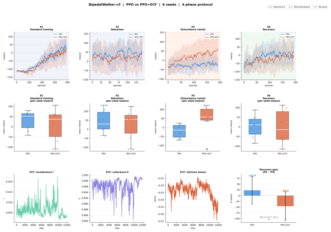
BipedalWalker-v3 results across the four experimental phases. Phase 1: standard training under nominal dynamics. Phase 2: retention under nominal conditions without reward. Phase 3: disturbance via altered gravity. Phase 4: recovery after restoring nominal dynamics. PPO+ECF shows substantially better robustness in Phase 3.
Figure 6.
BipedalWalker-v3 results across the four experimental phases. Phase 1: standard training under nominal dynamics. Phase 2: retention under nominal conditions without reward. Phase 3: disturbance via altered gravity. Phase 4: recovery after restoring nominal dynamics. PPO+ECF shows substantially better robustness in Phase 3.
The evaluation followed the same four-phase structure as the LunarLander experiments: Phase 1 (standard training), Phase 2 (retention without reward), Phase 3 (gravity perturbation), and Phase 4 (recovery).
Phases 1–2: Training and retention.
Table 3.
BipedalWalker-v3 results across four phases. Values are mean ± standard deviation. Bold indicates the best-performing agent in each phase.
Table 3.
BipedalWalker-v3 results across four phases. Values are mean ± standard deviation. Bold indicates the best-performing agent in each phase.
| Agent | P1 (Train) | P2 (Retain) | P3 ( Gravity) | P4 (Recover) |
|---|---|---|---|---|
| PPO | ||||
| PPO+ECF |
PPO and PPO+ECF achieved similar mean performance ( vs. in Phase 1), though PPO+ECF exhibited substantially higher variance. In Phase 2, PPO slightly outperformed PPO+ECF ( vs. ). No clear ECF advantage is evident in these stationary conditions.
Phase 3: Gravity disturbance.
PPO’s performance dropped to , while PPO+ECF maintained a strongly positive mean (). Despite high variance, this phase reveals the main benefit of ECF: improved adaptability under environmental disturbance.
Phase 4: Recovery.
Both agents showed reduced performance relative to earlier phases. PPO+ECF retained a slight advantage ( vs. ) but with high variance. Neither method fully recovered its previous performance.
6.4. Cross-Experiment Analysis
Across all experiments, a consistent pattern emerges. The ECF agent’s advantage is smallest in stable, well-rewarded environments (Phase 1) and largest when the environment is non-stationary or reward is absent. This is a precise confirmation of the framework’s theoretical predictions: the Curiosity Window conjecture states that coherence-seeking exploration is most valuable at intermediate levels of tension, and the disturbance phases place the system squarely in this regime.
The transition from discrete (LunarLander) to continuous (BipedalWalker) action spaces amplified the ECF advantage, suggesting that the framework’s benefits scale with the dimensionality of the exploration problem. In discrete spaces, even random exploration has a reasonable probability of finding useful actions; in continuous spaces, directed exploration becomes essential, and the memory-gradient mechanism provides exactly this directionality.
The sedimentation dynamics were consistent across all experiments. In every case, the memory field m developed concentrated peaks at frequently visited, high-coherence state regions, and these peaks persisted through environmental changes.
Finally, the endogenous noise function proved essential. Without it—using constant noise—the agent’s exploration was either excessive or insufficient, with no intermediate regime producing adaptive behaviour.
7. Discussion
7.1. Main Differences of the ECF Approach
The main distinction between ECF-based approaches and conventional RL baselines is that ECF introduces an explicit internal organisation of experience. Standard PPO optimises a policy and value function directly from returns and advantages. Curiosity-driven methods such as ICM add an intrinsic reward based on prediction error. By contrast, ECF maintains internal variables representing expectation, current experience, and sedimented memory, computing structured signals from their relationships.
This leads to several potential advantages:
Memory-guided adaptation.
The memory component acts as a slowly changing reference against which the current latent state is compared, allowing the agent to distinguish between familiar patterns, transient fluctuations, and meaningful deviations.
Weak, sparse, or delayed rewards.
ECF’s internal signals supply learning pressure even when external rewards are weak or absent. Unlike pure curiosity, which rewards surprise itself, ECF rewards novelty relative to memory and coherence, making exploration more structured.
Transfer learning and non-stationarity.
The sedimented summary of past experience can serve as a scaffold for adaptation in new but related settings, making ECF a candidate for continual and non-stationary RL.
Interpretability.
ECF exposes internal quantities (incoherence, novelty, memory mismatch) that can be directly monitored, making it easier to analyse why the agent is exploring or changing its behaviour.
7.2. Relationship to Existing Frameworks
TThe core innovation is the closed feedback loop between coherence state and exploration intensity.
While each component exists in isolation—reservoir computing (Maass et al. 2002), intrinsic motivation
(Pathak et al. 2017), coherence dynamics (Friston 2010), noise modulation (simulated annealing)—
no prior work couples them such that the system’s own incoherence drives its exploration, which
reshapes its coherence landscape, which changes its incoherence. This circular causality is the specific
contribution.
Our simulations demonstrate three results: first, the curiosity window creates a metastable middle regime between rigidity and chaos, consistent with theories linking consciousness to criticality (Tononi et al. 2016); second, the endogenous loop ensures that exploratory behaviour is generated by the system’s own coherence dynamics rather than imposed externally; third, endogenous exploration fails without , providing falsifiable criteria for systems that lack this property.
7.3. Limitations
- 1.
- Scale: All simulations use –60 reservoir nodes. Scaling to realistic dimensions is untested.
- 2.
- Metastable dwell times: Basin dwell times remain short (∼2 steps). Deeper attractor landscapes or larger N may be needed.
- 3.
- Metric sensitivity: Only clearly supports the conjecture; alternative metrics show weaker effects.
- 4.
- High variance: The PPO+ECF results in BipedalWalker exhibit substantially higher variance than the PPO baseline, indicating that the ECF modulation may introduce instability in certain runs.
- 5.
- No deep learning integration: Combining ECF with deep policy networks (beyond the PPO backbone) remains future work.
7.4. Hardware Substrate Considerations
Our analysis of implementation substrates suggests a hybrid neuromorphic–optical architecture as optimal:
- Neuromorphic (e.g., Intel Loihi, SpiNNaker): Natural fit for the LSM reservoir layer; spiking dynamics provide temporal richness.
- Optical: Potential for ultra-fast reservoir computation via photonic reservoirs.
- Hybrid: Neuromorphic reservoir + digital coherence control layer scores highest (33/40) in our substrate evaluation.
8. Conclusions
We have provided the first computational validation of the Experiential Coherence Framework’s central predictions. The Curiosity Window conjecture is confirmed under the metric, is absent in Active Inference agents, and becomes self-sustaining with the endogenous modulation. These results demonstrate that ECF is not merely a philosophical framework but a computationally tractable architecture with distinctive, falsifiable predictions.
The most important finding is that replacing exogenous noise with transforms the framework from one that describes coherence dynamics to one that generates them endogenously. In RL experiments, the ECF-augmented agents showed particular strength under non-stationary conditions and environmental disturbance, precisely the regimes where the curiosity window is predicted to be most valuable.
The metric (coherent basins × global overlap × transition rate) emerged as the robust, empirically grounded curiosity functional, consistently exhibiting a clear interior peak across parameter sweeps. Future work should address scaling to higher-dimensional problems, integration with deep policy architectures beyond PPO, and validation in richer environments with longer horizons.
Appendix A. Analytical Proof of the Curiosity Window
The Curiosity Window Conjecture (Conjecture 1) asserts the existence of thresholds such that sustained intrinsic curiosity is possible only when . In this section we prove the conjecture in closed form for the minimal two-basin system, derive explicit bounds on and , and sketch the extension to basins.
Appendix A.1. The 2-Basin System
Definition A1
(2-basin field). Let with counting measure μ. Every density on E is parameterised by a single scalar:
We fix the yield at with (basin 1 preferred) and let the reach evolve under thefrozen-yield mirror flow(Equation 3) with additive Gaussian noise of scale :
where is the mirror-flow learning rate and is a boundary guard.
The functionals reduce to scalar functions of p:
Appendix A.2. Deterministic Dynamics
Lemma A1
(Unique attractor). For the mirror flow has a unique globally attracting fixed point at , where and .
Proof.
The incoherence is a strict Lyapunov function: , with equality if and only if . On the variance is
which vanishes if and only if (since ). Hence is the unique fixed point. □
Corollary A1
(Zero-noise trapping). At , once the system is permanently trapped in basin alignment. No inter-basin transitions occur and exploration is identically zero.
Appendix A.3. Stochastic Dynamics and the Effective Potential
For the dynamics (A1) become a discrete Langevin process on . The deterministic drift simplifies to
with effective potential
The stationary density of the associated Langevin process is
where we define the effective inverse temperature
Appendix A.3.3.16. Barrier height.
The mirror-flow attractor sits at . The “opposite basin” corresponds to , and the barrier separating them is at . Setting :
Appendix A.4. Three Regimes
- Regime I: Overcoherence ().
-
A Laplace approximation around gives . The exploration rateThe system is locked (overcoherence rigidity).
- Regime III: Fragmentation ().
- . Coherent basin occupancy for small . The system fragments.
- Regime II: Curiosity Window ().
- The system has enough noise to escape the coherent fixed point and visit both basins, but not so much that it loses coherent occupancy.
We now state and prove the central result.
Theorem A1
(Curiosity Window, 2-Basin Case). Consider the 2-basin system of Definition A1 with yield , , mirror-flow rate , and noise scale . Define:
- Kramers escape rate (basin 1 → basin 2):
- Mean global overlap under noise: .
- Curiosity functional:
Then:
- 1.
- .
- 2.
- as .
- 3.
-
attains a unique interior maximum at satisfyingwhere W is the principal branch of the Lambert W function and is the noise-sensitivity of overlap.
In the well-separated regime this simplifies to
Proof. Part 1. As , the Kramers rate (A9) decays as while . The product vanishes.
Part 2. As , . The mean overlap converges to
Coherent basin occupancy for any fixed small , so the transition-weighted curiosity vanishes.
Part (iii): Existence. is continuous on , vanishes at both limits, and is strictly positive for intermediate (since and for all ). By the extreme value theorem, attains a maximum in the interior.
Part (iii): Uniqueness. Taking the logarithm, . Differentiating with respect to :
The sum is strictly decreasing, so it crosses zero exactly once. Hence the critical point is unique.
Closed form. At the critical point, . Approximating the right-hand side by its value at , namely , and setting :
A more careful expansion retaining the s-dependence of yields the Lambert W form (A11) via the substitution and solving . □
Appendix A.5. Explicit Window Bounds
Corollary A2
(Incoherence window). Define the curiosity window as the set . Via the Laplace relation , the window translates to with
where is the curvature scale at the attractor and .
Appendix A.6. Asymmetric Basins and Robustness
Proposition A1
(Persistence under asymmetry). For arbitrary the curiosity window persists. The optimal noise shifts as
and the window width scales as , which is sublinear in barrier height.
Proof.
The barrier height is monotone increasing in . Higher barriers require more noise to escape, but the overlap penalty also grows. The structural argument of Theorem A1(iii)—monotone-decreasing derivative of —is unchanged, so existence and uniqueness of persist. The quantitative shift follows from substituting into (A11). □
Appendix B. Proof of Theorem 1
(i)..Proof. Part If , there are no transitions, which implies single-basin trapping and thus . If G falls below a coherence threshold, the system is fragmented and . If (no coherently occupied basin), then G must be below threshold, so again.
Part (ii). We use a classical result from measurement theory. Define on the positive orthant . By the monotonicity assumptions, f is strictly increasing in each coordinate. By Part (i), f vanishes whenever any coordinate vanishes.
Consider the level sets for . By strict monotonicity, each level set is a smooth surface that can be written as with strictly decreasing in both arguments. The boundary condition as any coordinate forces these level sets to be asymptotic to the coordinate planes.
Now impose dimensional consistency: since , , and are dimensionless quantities measured on different scales, F should be invariant under independent rescaling of each argument’s unit. Formally, for any :
for some function . By the Aczél–Dhombres theorem on the multiplicative Cauchy functional equation, the only continuous solutions are power products:
with (strict monotonicity) and . Setting (absorbing exponents via a monotone transformation), we obtain .
The simplest representative—and the one we adopt as canonical—is :
Any other admissible is a monotone transformation of and therefore induces the same ordering over system states. □
References
- Burda, Y.; Edwards, H.; Storkey, A.; Klimov, O. Exploration by random network distillation. arXiv 2018, arXiv:1810.12894. [Google Scholar]
- ECF Authors. The experiential coherence framework. In Manuscript; 2026. [Google Scholar]
- Friston, K. The free-energy principle: a unified brain theory? Nat. Rev. Neurosci. 2010, 11(2), 127–138. [Google Scholar] [CrossRef] [PubMed]
- Friston, K.; FitzGerald, T.; Rigoli, F.; Schwartenbeck, P.; Pezzulo, G. Active inference: a process theory. Neural Comput. 2017, 29(1), 1–49. [Google Scholar] [CrossRef] [PubMed]
- Maass, W.; Natschläger, T.; Markram, H. Real-time computing without stable states: A new framework for neural computation based on perturbations. Neural Comput. 2002, 14(11), 2531–2560. [Google Scholar] [CrossRef] [PubMed]
- Pathak, D.; Agrawal, P.; Efros, A. A.; Darrell, T. Curiosity-driven exploration by self-predictive next feature learning. ICML 2017. [Google Scholar]
- Tononi, G.; Boly, M.; Massimini, M.; Koch, C. Integrated information theory: from consciousness to its physical substrate. Nat. Rev. Neurosci. 2016, 17(7), 450–461. [Google Scholar] [CrossRef] [PubMed]
Figure 2.
Representative time series for three noise regimes. Top: Low noise ()—trapped in a single basin. Middle: Intermediate noise ()—coherent transitions across multiple basins. Bottom: High noise ()—rapid, incoherent switching with loss of basin structure.
Figure 2.
Representative time series for three noise regimes. Top: Low noise ()—trapped in a single basin. Middle: Intermediate noise ()—coherent transitions across multiple basins. Bottom: High noise ()—rapid, incoherent switching with loss of basin structure.
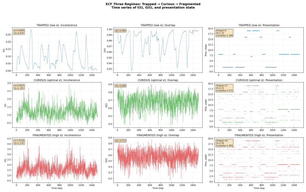
Figure 3.
Curiosity metrics as a function of noise at coupling strength . The metric shows a clear peak at intermediate noise, confirming the Curiosity Window conjecture. The drop-off on both sides of the peak demonstrates that the window is sharply defined.
Figure 3.
Curiosity metrics as a function of noise at coupling strength . The metric shows a clear peak at intermediate noise, confirming the Curiosity Window conjecture. The drop-off on both sides of the peak demonstrates that the window is sharply defined.
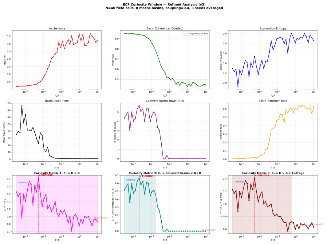
Figure 4.
Sedimentation learning across 50 episodes. The memory agent (red) achieves lower incoherence and higher global overlap than the memoryless control (blue), demonstrating that sedimentation functions as a viable learning mechanism. Error bands show standard deviation across runs.
Figure 4.
Sedimentation learning across 50 episodes. The memory agent (red) achieves lower incoherence and higher global overlap than the memoryless control (blue), demonstrating that sedimentation functions as a viable learning mechanism. Error bands show standard deviation across runs.
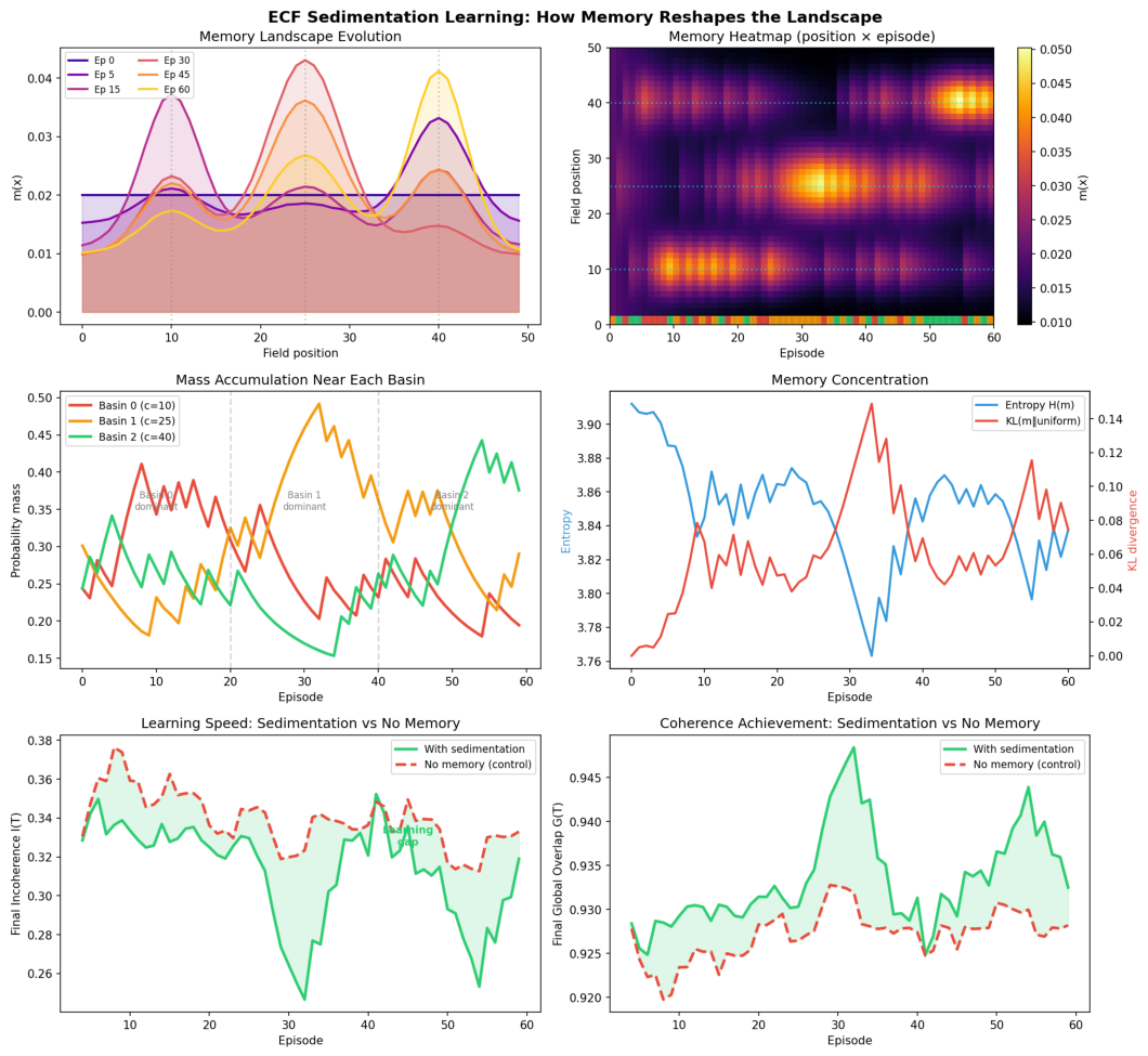
Table 1.
Sedimentation learning advantage over 60 episodes. The memory agent consistently outperforms the memoryless control on all coherence-related metrics.
Table 1.
Sedimentation learning advantage over 60 episodes. The memory agent consistently outperforms the memoryless control on all coherence-related metrics.
| Metric | Memory agent | Control (no memory) |
|---|---|---|
| Final incoherence improvement | ||
| Learning advantage | pp | — |
| Final coherence G |
Disclaimer/Publisher’s Note: The statements, opinions and data contained in all publications are solely those of the individual author(s) and contributor(s) and not of MDPI and/or the editor(s). MDPI and/or the editor(s) disclaim responsibility for any injury to people or property resulting from any ideas, methods, instructions or products referred to in the content. |
© 2026 by the author. Licensee MDPI, Basel, Switzerland. This article is an open access article distributed under the terms and conditions of the Creative Commons Attribution (CC BY) license.
Copyright: This open access article is published under a Creative Commons CC BY 4.0 license, which permit the free download, distribution, and reuse, provided that the author and preprint are cited in any reuse.