

Submitted:
19 August 2026
Posted:
20 August 2026
You are already at the latest version
Abstract
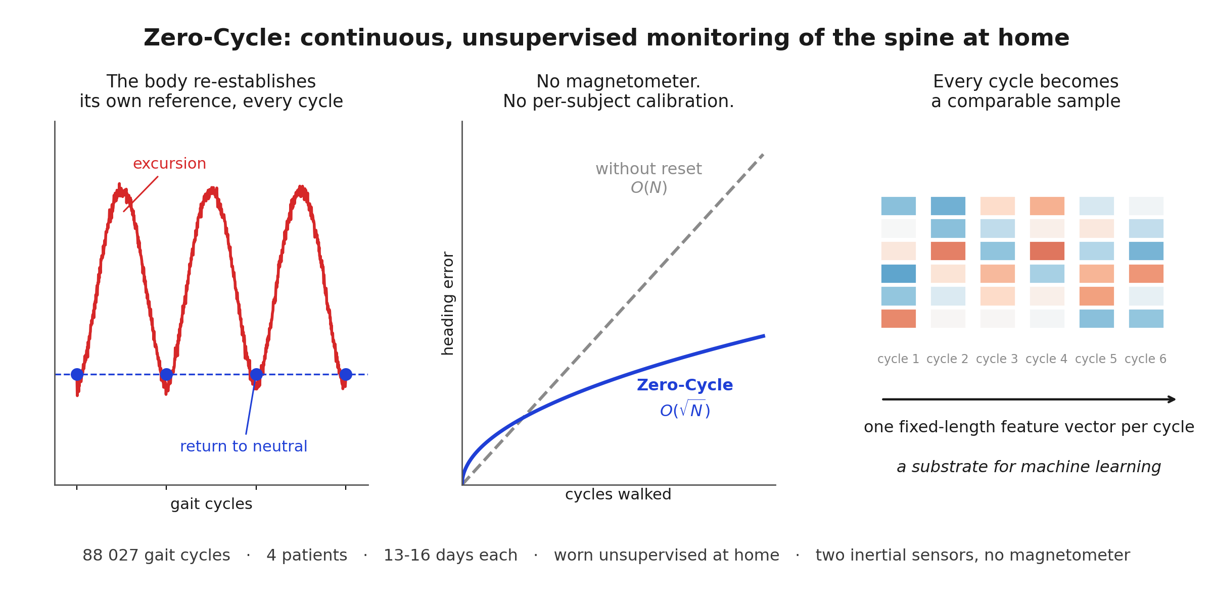
Continuous, objective records of spinal motion during ordinary life have not been available; assessment relies on intermittent questionnaires and brief supervised motion capture. A dual inertial-sensor garment applies the Zero-Cycle method, which treats the spine’s recurrent return to a consistent configuration once per gait cycle—present although no segment is ever stationary—as a body-intrinsic reference, emitting one fixed-dimensional feature vector per cycle. Resetting heading at each return bounds drift from linear growth to \( O(\sqrt{N}) \) and supplies the correction a magnetometer would otherwise provide, so no magnetic fusion is required; the per-cycle local frame removes subject-specific calibration. In a four-patient pilot conducted unsupervised at home, 88,027 cycles were analysed over 13 to 16 days each. The stream was stable over weeks and showed intervention-associated change, reported as Cliff’s delta with the cycle as the unit of analysis: sustained reduction in structural responders and none in a non-structural comparison case. The instrument was built to measure Dubousset’s cone of economy; the recording also contained a quantity that was not sought—the precision of the spine’s return to neutral, corresponding to Panjabi’s neutral zone, a complementary description of spinal control. The contribution is a substrate for machine learning rather than a more accurate sensor.
Keywords:
continuous monitoring
; home monitoring
; machine-learning substrate
; per-cycle features
; representation learning
; spine
; inertial measurement unit
; magnetometer-free
; drift correction
; cone of economy
1. Introduction
Disability and impaired function are hallmarks of spine pathology, but they are assessed clinically only at intervals—through questionnaires, the judgement of an experienced surgeon, and occasional laboratory motion capture—and not as a continuous record of how the spine actually moves during daily life. Such a record does not currently exist. The wearable inertial measurement unit (IMU) is the natural instrument for it, being inexpensive and unobtrusive, but continuous, unsupervised spine monitoring in the home has not been achieved.
What such a record should contain is less obvious than it appears. Spinal control is usually summarised by how far the spine moves, but two distinct descriptions of it already exist in the clinical literature. Dubousset described the cone of economy [1]: the envelope within which the trunk is maintained with least effort, an account of control as economy of excursion. Panjabi described the neutral zone [2,3]: the low-stiffness region about neutral within which the spine offers little resistance to motion, an account of control as the existence of a preferred configuration. The first concerns how far the trunk deviates; the second concerns where it comes back to. Neither has been measured continuously in a living person during ordinary activity, and they have not been measured together.
The reasons are well known. A recent validation of a spine-specific wearable against optical motion capture attributes the limited clinical adoption of single-sensor IMUs to three requirements—subject-specific calibration, drift correction, and high-fidelity sensor fusion [4]—the same problems identified across the inertial-sensing literature [5,6]. Orientation is obtained by integrating angular velocity, so gyroscope bias accumulates as heading drift; the usual correction, magnetometer fusion, is unreliable indoors and near metal; and features computed in the sensor frame shift with each donning and with garment slip, which is why such systems typically require per-subject calibration and degrade outside the laboratory.
A fourth requirement is logically prior to these three and is rarely stated: what quantity should be measured. The three above concern how faithfully a chosen quantity is recovered, and they presuppose that the quantity is range of motion, a joint angle, or a segmental moment—measurands inherited from goniometry and from optical gait laboratories. None of them is defined by the body itself; each requires an external frame to be meaningful, which is what makes calibration and fusion necessary in the first place. The measurand used here was not chosen from that inventory. The instrument was built to capture Dubousset’s cone of economy [1], the envelope within which the trunk is held with least effort—a construct that is body-referenced rather than laboratory-referenced, and which motivated a differential thoracic-against-pelvic architecture rather than a single-sensor one. The per-cycle return to a body-determined configuration emerged from that recording, first as the mechanism by which heading drift could be bounded without a magnetometer, and only subsequently as a quantity in its own right. That the removal of calibration, drift, and fusion follows from the measurand rather than from improved estimation is therefore a consequence of the architecture, not a design premise, and it is stated here because it is the more general lesson. What the recording also contained was the second of the two descriptions above: the spine’s return, cycle after cycle, to a narrow region about neutral. The cone was sought; the neutral zone was found alongside it, and the two proved complementary rather than alternative.
It is worth stating the novelty precisely, because several adjacent literatures already exist. Continuous home-based movement monitoring is established in neurological and rehabilitation settings, where wearable inertial systems track motor symptoms and physical activity over extended periods [7]. Spine-specific inertial work has largely addressed different problems: validation of trunk kinematics during supervised or standardized functional tasks [4,8,9,10,11], automated spine-angle estimation for telerehabilitation and prompted exercise [12], and the repeatability of spinal-posture measurement in daily life [13]. These studies establish that spine kinematics can be measured with IMUs and that home use is attractive, but none provides a continuous, unsupervised, at-home stream of spine-specific kinematic control sampled at the level of individual movement cycles across an intervention course. The present claim is therefore deliberately narrow: not that home wearables, posture sensors, gait monitors, or spine IMUs are new, but that continuous, unsupervised, at-home, per-cycle monitoring of spine-specific kinematics, demonstrated through an intervention course, is the specific paradigm reported here.
This paper reports, to our knowledge, the first continuous, unsupervised, multi-week recording of spinal motion in the home, obtained with a dual-IMU garment and the Zero-Cycle method. The method uses the periodicity of gait: the differential trunk–pelvis configuration returns to a consistent neutral configuration approximately once per gait cycle, even though no segment is ever stationary, and this recurrent return is used as a body-intrinsic reference, producing one fixed-dimensional feature vector per gait cycle. Almost incidentally, the same reference removes the three problems above, two of them through one mechanism: resetting the estimate at each return bounds heading drift to and, because the reset supplies the heading correction a magnetometer would otherwise provide, removes the need for magnetic fusion, while six-axis gyroscope–accelerometer fusion is retained; the per-cycle local frame removes subject-specific calibration. This reference also differs from the zero-velocity update, which requires a momentary stop and is therefore limited to the foot whereas the trunk never stops; that distinction is developed in Section 2.2.
The substance of the contribution is what this recording is: a rich substrate for machine learning. Each gait cycle yields a fixed-dimensional sample, and because every sample is expressed in a frame comparable across sessions and subjects without calibration, the per-cycle stream has the properties that learning systems require and wearable data usually lack. It is approximately stationary, the per-cycle reset removing the monotonic drift a model would otherwise fit. It carries little frame-related distribution shift from donning or slip, because the frame is re-established each cycle, so a model trained on one recording or one patient applies to the next without recalibration. It is uniformly segmented, one sample per cycle with the per-cycle return as a natural boundary, which maps directly onto sequence models, and cycles in which the return fails are retained as informative samples rather than discarded. It is reproducible, fixed to a single versioned extractor. And it is produced without labels: a two-week recording yields on the order of tens of thousands of samples to which sparse labels—clinical timepoints, patient-initiated events, longer-term outcomes—attach at the timestamp, so the stream is suited to self-supervised pretraining with light supervision. This substrate, rather than a more accurate sensor, is the result we present.
The contributions are, in order: (i) the first continuous, unsupervised, multi-week recording of spinal motion in the home; (ii) its formulation as a per-cycle machine-learning substrate with the stationarity, frame-invariance, uniform-segmentation, and version-pinning properties above—the principal contribution; (iii) the Zero-Cycle measurement that produces it, drift-stabilised and magnetometer-free, which removes calibration, drift, and fusion through a single body-intrinsic reference and is distinct from the zero-velocity update; and (iv) a four-patient pilot showing that the stream is stable over weeks and shows intervention-associated temporal change, including a within-study non-responder comparison case, assessed by internal drift-consistency criteria rather than external ground truth. The two per-cycle quantities correspond to the two descriptions of control set out above: the excursion about neutral to Dubousset’s cone of economy, which the instrument was built to capture, and the precision of the return to Panjabi’s neutral zone, which was not anticipated. The relation between them is discussed as interpretation rather than as a validated measurement, and the pilot is not powered to establish whether the two vary independently. The engineering analysis and long-distance validation of the drift correction are in a companion letter [14]; a phenotype model is not developed here.
More broadly, the principle is not specific to the spine. We propose that the natural computational unit of free-living biomechanics is not the timestamped sensor sample but the biomechanically anchored movement cycle: expressing each cycle in a body-intrinsic frame and emitting it as a fixed-dimensional token defines a representation layer between wearable hardware and machine learning, on which movement phenotypes and outcome models can be learned. The spine is used here as its first continuous, unsupervised, in-home demonstration; the same construction is applicable, in principle, to other quasi-periodic segmental motion, such as the knee, the hip, or gait as a whole.
2. Materials and Methods
2.1. Instrumentation
Two BNO085 sensors were worn over the upper thoracic spine (approximately T1) and the sacrum (approximately S1), about 50 cm apart, in a soft garment intended for continuous home wear (Figure 1). The two-sensor differential configuration was adopted so that trunk excursion could be expressed against the pelvis rather than against a room, following Dubousset’s cone of economy [1]; the per-cycle return properties described in Section 2.4 were not anticipated at the design stage. Each sensor operated in a gyroscope-plus-accelerometer (six-axis) fusion mode with the magnetometer disabled, so that pitch and roll are gravity-referenced while heading is unconstrained and corrected by the per-cycle reset. Data were sampled at 100 Hz; the higher rate resolves the brief return to the neutral configuration and the fine structure of each cycle that a lower rate does not, an effect examined directly for inertial spine-orientation estimation in [15]. The sensors cost on the order of a few euros each.
2.2. Drift and the Zero-Cycle Reset
Standard orientation estimation integrates angular velocity continuously,
so the bias term b grows in proportion to elapsed time. Because the trunk never reaches a true zero-velocity state during gait, the zero-velocity update [16,17] that bounds foot-mounted navigation is inapplicable. The Zero-Cycle reference is instead a kinematic configuration the segment returns to, and the method operates entirely in the orientation domain: it does not double-integrate acceleration to recover position, and so does not incur the velocity error the zero-velocity update exists to remove. At each return, the reset is computed as the relative rotation in quaternion form, taking the orientation at the cycle start as the reference,
and the per-cycle increments are accumulated. Because the composition is carried out in quaternion algebra, with Euler extraction applied only to the small per-cycle relative rotation, the procedure is free of gimbal-lock artefacts. When the per-cycle increments are zero-mean and approximately independent, the cumulative heading error follows a random walk,
in place of the linear growth of Equation (1). The per-cycle return to neutral responsible for this drift scaling is also the bracket of the analysis: the same event that recalibrates the estimate delimits the cycle within which the per-cycle quantities below are taken.
2.3. Differential Spine Motion
Spinal motion is computed as the orientation of the thoracic sensor relative to the pelvic sensor,
so that whole-body turning, common to both sensors, cancels in the differential and leaves the three inter-segmental components—flexion/extension, lateral bending, and axial rotation—the last of which is inaccessible to a single magnetometer-free sensor.
2.4. Local Neutral Detection and the Body-Intrinsic Frame
Within confirmed walking bouts—identified by a heel-strike detector (2 Hz Butterworth pre-filter, peak prominence, and a walking-bout coefficient-of-variation gate) validated in the companion letter [14]—the differential orientation is monitored, and a per-cycle reference is estimated as the geodesic median of the heel-strike samples in a short rolling window,
A per-cycle sample qualifies as a reset anchor when its rotation-vector representation lies within a fixed tolerance of this local neutral. At each anchor the differential quaternion is snapped to identity, defining the local frame for the subsequent cycle,
where d is the geodesic angle of the local-frame orientation. Referring each cycle to its own freshly established local neutral is the step that makes the measurement insensitive to slow garment or mounting drift within a recording (12–35°/h) and to differences in sensor placement between recordings (70–100°). Standing cycles are bridged by interpolating the local neutral between consecutive walking bouts when the wearer remains continuously upright; sitting and lying cycles receive no kinematic measurement and are logged for activity allocation only. The return criterion is defined by the recorded distribution of differential orientation at heel strike rather than by a modelled or externally specified neutral posture; no anatomical or biomechanical construct enters the detector. A single frozen version of this extractor was used for every file in the study.
2.5. The Per-Cycle Feature Vector and the Substrate Stream
For each cycle, two primary quantities are taken in the local frame. The valley is the geodesic distance of the cycle’s return sample from the local neutral, a measure of how precisely the spine returns,
and the peak is the per-cycle excursion, the maximum geodesic distance from the local neutral over the stride,
Their difference is the inter-segmental dynamic range. Two further channels are recorded: the return accessibility , the retained outcome of the gating event (whether the cycle reached the local neutral within tolerance), and the dwell and within-zone wobble , which quantify how long and how much the spine moves while near neutral. Assembled per cycle and stacked over a recording, these define the substrate object,
Each row of X is one cycle; the rows are ordered on a regular per-cycle grid and carry their wall-clock timestamp, cycle duration, and bout identifier, and the per-cycle return marks the boundary between them. X, not the sensor, is the deliverable of this work.
For reference, the following terms are used throughout. The Zero-Cycle anchor is the recurrent biomechanical configuration (Equation 5) used as an endogenous reference in place of an external calibration. Cycle canonicalisation is the expression of each movement cycle relative to its contemporaneous anchor (Equation 6). The Zero-Cycle token is the fixed-dimensional feature vector emitted for one cycle (Equation 9). The Zero-Cycle substrate is the ordered sequence X of these tokens together with their timestamps, bout identifiers, quality indicators, and extractor version. Biomechanical tokenisation denotes the conversion of a continuous wearable recording into this sequence of naturally segmented, body-referenced units.
2.6. Suitability as a Machine-Learning Substrate
Four properties of X follow directly from its construction and together make it suitable as a learning input.
Approximate stationarity. The drift scaling (Equation 3) removes the monotonic trend that a model would otherwise fit in place of biology; the per-cycle feature distribution is approximately stable across a recording, conditional on biomechanical state, so day-to-day comparisons reflect physiology rather than accumulated sensor error.
Frame invariance and reduced distribution shift. The snap-to-identity local frame (Equation 6) removes donning angle and within-file slip, so a feature vector computed on one day, or in one patient, is directly comparable to another without per-subject calibration. This is the property that normally forces recalibration or explicit domain adaptation in wearable pipelines; here it is built into the measurement, which supports cross-session comparability and, in principle, cross-subject generalization, a property the present data do not test.
Uniform tokenization. Fixed-dimensional rows on a regular per-cycle grid, with the per-cycle return as a natural boundary token, map directly onto temporal-convolutional and attention architectures; the cycle is the token and the return is the segmentation marker. Retained failed returns enter the sequence as informative tokens rather than being dropped.
Version-pinned reproducibility. A single frozen extractor yields deterministic, versioned feature definitions. This is an operational and regulatory requirement as much as a scientific one: features must be defined identically across training, validation, and deployment, and because the biomarkers are detector-version-dependent, the extractor version is pinned and never mixed across comparisons.
Finally, the representation is produced unsupervised. Labels—clinical timepoints, patient-initiated pain-button events, and longer-term outcomes—attach at the timestamp level, so the large number of unlabelled per-cycle samples per patient over a two-week recording supports self-supervised pretraining with light supervised fine-tuning.
2.7. Cohort and Protocol
Four patients were monitored. The index patient (Z) was an 80-year-old with severe L3/L4 sciatica treated with transforaminal epidural steroid injection (TESI). A second TESI patient (P) presented with sciatica for which MRI showed no corresponding lesion, and serves as a within-study comparison case. Two further patients (F and K) underwent single-level foraminotomy. Each patient wore the device continuously in their own home, unsupervised: Z for 13 days (4–18 February 2026), K for 16 days (9–26 March 2026), P for 16 days (10–25 March 2026), and F for 16 days (14–29 April 2026). Patient-reported outcomes were recorded at the first and last day of each patient’s monitoring period using the Oswestry Disability Index (ODI) and the Core Outcome Measures Index (COMI). A single frozen extractor version was used for all four recordings; the version identifier is recorded with the analysis code.
2.8. Analysis
The unit of analysis was the movement cycle. Recording days yielding fewer than 200 validated cycles were excluded, because the daily metric defined below is undefined below that count; four such days were removed across the cohort, two of which also showed a median sensor tilt above 50°, indicating that the device was off the body. The four recordings together contributed 88,027 analysed cycles (Z 19,133; K 38,210; P 17,959; F 12,725). The clinical sample is four patients, and the cycle is used as a descriptive unit within each patient rather than as an independent observation; because adjacent cycles are serially correlated and nested within bouts, days, and patients, no population-level significance test is appropriate and none is reported. Within-patient effect sizes were instead reported as Cliff’s delta, computed for each patient between a pre-intervention window and the post-intervention plateau against that patient’s own distribution,
Cliff’s delta is a non-parametric measure of dominance bounded between minus one and one and makes no distributional assumption [18]. It is oriented here so that a positive value indicates a reduction of the per-cycle metric after intervention, i.e., pre-intervention values stochastically dominate post-intervention values.
Daily metric and independence from activity. For day-to-day comparison the per-cycle stream is summarised with a fixed-size window rather than a whole-day average: on each day the most compact 200 consecutive cycles are taken, and the median peak and median valley of that window—the Best-200 metric used in Figure 3—are reported. The fixed window size makes a light-activity day and a heavy-activity day contribute the same number of cycles, and taking the most compact window reflects the best-controlled state the spine reached that day rather than an average diluted by fatigue or by long, variable walking bouts. The control for activity is therefore structural rather than statistical: because the window is a fixed 200 cycles, a light day and a heavy day contribute the same number of cycles to the daily value, and the metric cannot be inflated merely by walking more. Consistent with this, across 45 plateau patient-days pooled within patient, the daily valley and peak showed no detectable association with distance walked, walking time, or cycle count (Spearman , all ). A sample of this size cannot establish independence, and the absence of a detected association is not evidence that none exists; the claim made here is the weaker one that the intervention-associated changes reported below are not accounted for by the activity differences present in this cohort. All four patients remained ambulatory throughout, so the metric was not evaluated under conditions approaching immobility, where too few cycles would be available for the window to be defined at all.
2.9. Validation
Concurrent optical motion capture was considered and deliberately not used. The reason is primarily one of measurand rather than of logistics. Optical capture expresses kinematics in an external laboratory frame defined by marker positions, whereas the quantity measured here is defined against a body-intrinsic reference that the spine re-establishes on each cycle; agreement between the two would therefore be a comparison between different quantities, and disagreement would not adjudicate either. Second, the property that matters cannot be observed inside a capture volume. Per-cycle drift stabilisation is a statement about behaviour over thousands of consecutive cycles: absolute heading error grows as rather than linearly, so error relative to distance travelled falls as , and the sampling precision of the per-cycle statistics improves as more cycles are accumulated. A capture volume admits a few consecutive cycles of prompted walking and can neither exhibit that scaling nor sample the free-living behaviour in which the measurement is intended to operate. Third, validation of spine-worn inertial sensing against optical capture during supervised functional tasks has already been reported [4]; repeating it would establish agreement on the supervised, laboratory-frame measurand that this work does not use. The angular accuracy of the differential trunk–pelvis measurement against an external standard remains a separate and legitimate question, and is addressed in planned work; it is distinct from validating the per-cycle measurand, which is why the criteria below are internal.
Loop-closure error, the conventional figure of merit for dead reckoning, is insufficient on its own: when reset timing is correlated with the underlying drift, closure can be artificially small even when the reconstructed path is wrong. The per-cycle stream was therefore assessed for internal drift consistency by its random-walk signature—approximately zero-mean per-cycle increments, near-zero lag-one autocorrelation, and cumulative heading contained within a envelope—and by recovery of a reference per-cycle return dispersion (approximately 1.85°) established on the same hardware in separate recordings [14]. Both criteria are available without external ground truth, which is what makes them suitable for unsupervised wear.
3. Results
3.1. Overview
Across the four patients, 88,027 movement cycles were analysed over 13 to 16 days of monitoring each, entirely in the free-living home setting and without a magnetometer. The per-cycle stream remained drift-stabilised throughout, satisfying the random-walk signature described above, so that day-to-day comparisons of the per-cycle features reflect biomechanics rather than accumulated sensor error. The result is therefore a monitoring result rather than a single task result: one extractor produced an ordered sequence of comparable cycle-level measurements throughout ordinary home activity, and the clinical course appears as a distributional process—the per-cycle band narrows, widens, fragments, or stabilises over time—rather than as a difference between two scalar values.
3.2. The Per-Cycle Stream
Figure 2 shows the per-cycle stream for the index patient across the monitoring period. In each panel, every gait cycle contributes two values plotted against cycle count: the within-cycle excursion from neutral (peak) and the return position, the distance of the cycle’s return from the local neutral (valley). The panels correspond to successive recording sessions, from the pre-treatment baseline through the post-injection course; each session contains several hundred to several thousand cycles recorded continuously during unsupervised home wear. The separation between the two bands and the dispersion within each band are the per-cycle quantities summarised in the analyses that follow, and the figure shows that they are defined at the level of individual cycles rather than as session averages. Across the sequence of sessions the bands change systematically: in the baseline and pre-treatment sessions both bands are high and broad, and in the later sessions the valley band moves toward zero and narrows, indicating a more precise and more consistent return to neutral. This progression is quantified below.
3.3. Clinical Course Across the Cohort
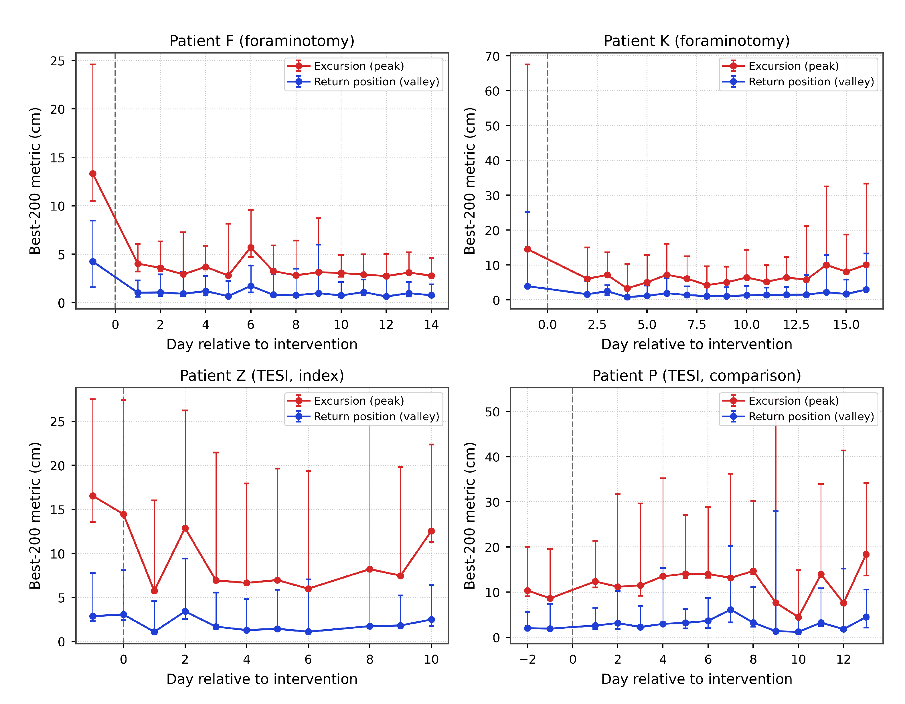
Figure 3 summarises the four patients using the Best-200 daily metric: for each recording day, the median peak (excursion) and median valley (return position) of the most compact 200-cycle window of that day, plotted against day relative to intervention. The two foraminotomy patients (F and K) and the index TESI patient (Z) show a reduction of the per-cycle metric around the intervention that is then maintained; in patient Z the metric re-widens after approximately day ten. The second TESI patient (P), whose sciatica had no corresponding lesion on MRI, shows no such reduction. Error bars are the inter-quartile range of the per-cycle distribution within each day.
Two recordings show a late partial re-widening of the metric, and the two occur in opposite activity contexts. In patient Z the re-widening over the final days coincided with a fall in walking volume rather than a rise (mean 367 m per day over the last two days, against 2086 m per day over days six to eleven), so it cannot be an artefact of increased exposure; its attribution to a concurrent hip process is clinical and is not established by the present data. In patient K the re-widening coincided instead with the highest walking volumes of that recording (mean 6167 m per day over the final four days, against 2992 m per day earlier), consistent with a return to unrestricted activity, although the single highest-distance day before the re-widening carried a tight metric (6089 m, peak median 7.2 cm), so walking volume alone does not account for it. Neither explanation is tested by this design, and both are reported as observations rather than as findings.
Figure 3.
Four-patient Best-200 trajectories. For each patient, the median excursion (peak, red) and median return position (valley, blue) of the most compact 200-cycle window are plotted against day relative to intervention (dashed line); error bars are the within-day inter-quartile range. Patients F and K underwent foraminotomy; patients Z and P received transforaminal epidural steroid injection. The structural responders (F, K, Z) show a reduction of the per-cycle metric that is maintained, with a late re-widening in Z; the non-structural case (P) shows no change at the intervention. Display units are centimetres of the Best-200 metric.
Figure 3.
Four-patient Best-200 trajectories. For each patient, the median excursion (peak, red) and median return position (valley, blue) of the most compact 200-cycle window are plotted against day relative to intervention (dashed line); error bars are the within-day inter-quartile range. Patients F and K underwent foraminotomy; patients Z and P received transforaminal epidural steroid injection. The structural responders (F, K, Z) show a reduction of the per-cycle metric that is maintained, with a late re-widening in Z; the non-structural case (P) shows no change at the intervention. Display units are centimetres of the Best-200 metric.
3.4. Intervention-Associated Change and Effect Sizes
The trajectories in Figure 3 are quantified as per-patient effect sizes in Table 1. The patients with structural pathology (Z, F, K) have positive Cliff’s delta (, , ), corresponding to a reduction of the per-cycle metric that is maintained, while the non-structural comparison case (P) has a near-zero negative value (). This comparison case is particularly informative: a measurement that does not change when there is no structural change to detect supports the interpretation of the measurement in the cases where it does change. As an example of the underlying per-cycle channels, the post-operative course of patient K, processed through the frozen extractor, showed the daily valley median falling from 14.9 cm on the pre-operative day to a plateau median of 2.0 cm () and the peak median from 48.6 cm to 8.5 cm (). The plateau was established by the first post-operative recording day and held for eleven days before the late re-widening described above; the two channels moved together and by similar proportions rather than on separate time courses.
The structural classification used above is radiological rather than symptomatic. Both TESI patients presented with sciatica; they differ in that the index patient had lateral recess stenosis at the symptomatic level on MRI before treatment (Figure 4), whereas patient P had no corresponding lesion. That distinction, and not the presenting complaint, is what separates them.
3.5. Relation to Patient-Reported Outcomes
Patient-reported outcomes for the same monitoring periods are given in Table 2. All four patients reported large improvement on both instruments: ODI fell by 34 to 56 percentage points and COMI by 2.4 to 6.7 points, and every patient moved from the severe or worse category to minimal or moderate disability. The per-cycle measurement agrees with that improvement in three of the four. In the fourth, the non-structural comparison case P, the questionnaires record a change of the same magnitude as the others—ODI 46% to 12%, COMI 6.0 to 1.4—while the per-cycle metric does not shift. The instrument and the questionnaires therefore separate one patient of four, and they separate the patient in whom no structural lesion was identified. A single case is an observation and not a rate, and the direction of the disagreement cannot be adjudicated without longer-term outcome data; it is reported because the capacity to disagree with a questionnaire is the property that would make continuous measurement useful, and because a measurement that agreed with the questionnaire in every case would add nothing to it.
3.6. Quantities Defined only at the Per-Cycle Level
Two further quantities are defined at the per-cycle level and are not recoverable from session averages. The first is return accessibility, the fraction of cycles that reach the local neutral within tolerance, which varies independently of excursion magnitude: in patient K it increased from 9% to 32% over six days while the excursion median decreased, indicating that the rate of successful return and the precision of return follow different time courses. The second concerns the structure of motion around the local neutral. Distinguishing the scatter of the return point (return precision) from the residual motion while near neutral and the time spent there, the index patient after treatment showed a large reduction in return scatter (from 11.7 to 2.3 units) together with an increase in near-neutral motion and dwell time (0.76 to 1.08 units and 0.25 to 0.86 s, respectively). These quantities are determined by the per-cycle structure rather than by a daily summary, and depend on retaining all cycles, including those in which the return failed. They are candidate features for a learning model and are not available from a session-averaged or drift-affected pipeline.
4. Discussion
The principal contribution is the per-cycle representation rather than the sensor or its accuracy: a stable, calibration-free description of spine movement obtained over weeks in the home setting rather than in a brief supervised session. The reference that produces it—the spine’s recurrent return to a consistent configuration each cycle—is what makes continuous trunk measurement feasible, since the trunk provides no stationary interval for the conventional correction, and it removes calibration, drift, and magnetic fusion as a secondary consequence rather than as the objective.
The most important property for machine learning is frame invariance. Referring each cycle to its own local neutral reduces the donning and slip that otherwise introduce a frame-related distribution shift in sensor-frame features, stabilising the input distribution at the source. This supports, in principle, transferring a model trained on one cohort to another without per-subject recalibration, and is a stronger property than post-hoc normalisation because the invariance is a property of the measurement rather than of a fitted correction.
Using the cycle as the unit of representation is suited to sequence models: regularly ordered, fixed-dimensional samples with a defined boundary correspond to the inputs such models expect [19], with the per-cycle return serving as the segmentation boundary. Retaining cycles in which the return failed, and recording the precision of return, preserves information discarded by a reset-only pipeline; the distribution of return success and precision is itself a feature.
The representation is produced without labels, which supports label-efficient training: the large number of unlabelled per-cycle samples per patient over a two-week recording is suitable for self-supervised pretraining [20,21], with sparse labels—patient-initiated pain events, clinical timepoints, and six- to twelve-month outcomes—applied at the corresponding timestamps. Monitoring of this kind is likely to be most informative where it disagrees with questionnaire scores; discordance with patient-reported measures is itself of interest rather than a limitation of the instrument. The present cohort contains one such case. Patient P reported an improvement indistinguishable in magnitude from the three patients with structural pathology, and moved from severe to minimal disability on both instruments, while the per-cycle measurement did not move at all (Table 2). Which of the two is the better guide to that patient’s course cannot be settled here and requires longer follow-up. What the case does establish is that the two do not measure the same thing, which is the precondition for the measurement adding anything.
The two per-cycle quantities correspond to the two established descriptions of spinal control, and the relation between them is the least expected result of this work. The excursion about neutral corresponds to Dubousset’s cone of economy [1], the envelope within which the trunk is maintained with least effort, measured here once per cycle rather than as a static posture; this is the quantity the instrument was built to capture. The precision of the per-cycle return was not sought. It appeared as the observation that the differential orientation reoccupies a narrow region at each cycle, with a scatter that is stable within a recording and that changes after intervention; the correspondence to Panjabi’s neutral zone [2,3], the low-stiffness region about neutral, was recognised subsequently. That construct was defined from cadaveric segmental testing under applied load, and the present quantity is neither a measurement of segmental stiffness nor a validation of it—the correspondence is offered as an interpretation, and establishing it formally would require concurrent reference standards we did not collect.
The two descriptions are complementary rather than competing. One concerns how far the trunk deviates over the cycle, the other where it comes back to; a controller may economise on excursion, on the precision of its return, or on both, and the clinical meaning of the two need not be the same. Whether they vary independently is not settled here, and the present data do not settle it: in the post-operative patient the two channels fell together and by similar proportions (% and %), and no recording in this cohort shows one moving while the other does not. Establishing whether the two carry independent clinical information requires a cohort in which they can be compared across patients rather than within four. These interpretations motivate the quantities but are not required for the substrate argument, which rests only on the per-cycle stream being stable, comparable, and informative.
This representation is intended as the input layer for downstream tasks: movement phenotyping, prediction of symptom flares and longer-term outcomes, and automated generation of structured progress notes from the per-cycle stream. Because the recording is continuous and unsupervised, the same stream also supports discrimination of activities of daily living—posture and activity states such as sitting, standing, walking, and the transitions between them—directly from the worn sensors and without supervision [20,22]; this supplies the behavioural context in which the per-cycle kinematic features are read, and is the subject of concurrent work rather than of this paper. The present cohort shows distinguishable response patterns—a sustained reduction in the structural responders and no change in the non-structural case—which indicates the direction the representation supports rather than a phenotype classification established here. A single-sensor configuration is also possible: a single trunk sensor returns to its own per-cycle neutral and can provide a heading estimate and per-cycle return features, without the differential inter-segmental kinematics that two sensors provide.
5. Limitations
This is a pilot of four patients, and all comparisons are within-subject across days rather than between subjects; the frame-invariance argument supports cross-subject comparability in principle, but the present data do not test it. A study of this size estimates the magnitude of the within-patient effect and establishes feasibility; it does not test a hypothesis, and no inference about a population is drawn from it. The quantity that determines the size of a confirmatory study is the between-patient variance of the pre-to-post change, and four patients do not estimate it usefully, so no power calculation is offered here. The per-patient effect magnitudes in Table 1 are reported partly so that they can serve as the input to that calculation. The confirmatory study is designed with several days of monitoring both before and after intervention, with the readout criteria and the primary endpoint stated before enrolment, and with the extractor version frozen in advance. Optical motion capture was not used, for the reasons given in Section 2.9; the angular accuracy of the differential measurement against an external standard is consequently unestablished and is the subject of planned validation. The correspondence of the two per-cycle quantities to Panjabi’s neutral zone and Dubousset’s cone of economy is interpretive and was not validated against those original constructs; nor does the pilot establish whether the two quantities vary independently. Loop-closure error must be interpreted with care and was not used as a primary metric. The return-detector parameters—the tolerance and the rolling-window length—were fixed rather than optimised. Because the features are detector-version-dependent, the extractor must be frozen, its version reported, and versions never mixed across comparisons. The pre-intervention window rests on a single recording day in the two surgical patients and on part of one further day in the index patient, so each effect size compares one baseline day against a multi-day plateau; the baseline distribution is correspondingly poorly characterised, and a design with several days of monitoring before as well as after the intervention is the subject of the next study. One recording contained a mounting artefact, which was flagged rather than filtered; as it adds scatter to the pre-intervention window, it can only reduce the measured effect and so does not inflate the reported result.
6. Conclusions
We have presented the first continuous, unsupervised, multi-week recording of spinal motion in the home, and its principal property: a per-cycle stream suitable as a substrate for machine learning. Using the spine’s recurrent return to a consistent configuration as a body-intrinsic reference produces, once per gait cycle, a fixed-dimensional feature vector that is stationary, comparable across sessions and subjects without calibration, uniformly segmented, and version-pinned, and, as a secondary consequence, removes the drift, calibration, and magnetic-fusion problems that have limited wearable spine IMUs. In four patients across two intervention types in the unsupervised home setting, the stream was stable over weeks and showed intervention-associated temporal change, showing a sustained reduction in the structural responders and no change in a non-structural case. The work began as an attempt to measure Dubousset’s cone of economy continuously, and returned a second quantity that was not sought: the precision of the spine’s per-cycle return to neutral, corresponding to Panjabi’s neutral zone. The two are complementary descriptions of spinal control—the envelope of excursion, and the configuration that excursion is organised about—and this is the first setting in which both have been recorded together during ordinary life. Whether they carry independent clinical information is a question for a cohort rather than for four patients. The contribution offered here is the substrate itself and its suitability for movement phenotyping and outcome models; development of that layer is the subject of future work.
Patents: International patent applications covering the Zero-Cycle measurement method and its application to segmental biomechanical monitoring are pending.
Author Contributions
Conceptualization, G.M.; methodology, G.M.; software, G.M.; validation, G.M. and T.S.; formal analysis, G.M. and A.P.; investigation, G.M., T.S. and A.P.; data curation, G.M.; writing—original draft preparation, G.M.; writing—review and editing, G.M., T.S. and A.P.; project administration, A.P. All authors have read and agreed to the published version of the manuscript.
Funding
This research received no external funding.
Institutional Review Board Statement
The study was conducted in accordance with the Declaration of Helsinki and approved by the Bioethics Committee of the Lower Silesian Medical Chamber in Wrocław, Poland (Komisja Bioetyczna przy Dolnośląskiej Izbie Lekarskiej we Wrocławiu), Resolution No. 32/BNBO/2025 of 8 October 2025.
Informed Consent Statement
Informed consent was obtained from all subjects involved in the study. Written informed consent has been obtained from the patient and from the individual shown in Figure 1 to publish this paper.
Data Availability Statement
The original data presented in the study are openly available in the Zero-Cycle Spine directory of https://github.com/gmiekisiak/spinerebel, together with the analysis pipeline and the frozen extractor version used for every recording in this study.
Acknowledgments
During the preparation of this manuscript, the authors used Claude (Anthropic) for minor language editing. The authors have reviewed and edited the output and take full responsibility for the content of this publication.
Conflicts of Interest
G.M. is an inventor on pending international patent applications covering the measurement method described in this work and has a financial interest in its commercialisation. T.S. and A.P. declare no conflicts of interest. The funders had no role in the design of the study; in the collection, analyses, or interpretation of data; in the writing of the manuscript; or in the decision to publish the results.
References
- Dubousset, J. Three-dimensional analysis of the scoliotic deformity. In The Pediatric Spine: Principles and Practice; Weinstein, S.L., Ed.; Raven Press: New York, NY, USA, 1994. [Google Scholar]
- Panjabi, M.M. The stabilizing system of the spine. Part II. Neutral zone and instability hypothesis. J. Spinal Disord. 1992, 5(4), 390–396. [Google Scholar] [CrossRef]
- Panjabi, M.M. The stabilizing system of the spine. Part I. Function, dysfunction, adaptation, and enhancement. J. Spinal Disord. 1992, 5(4), 383–389. [Google Scholar] [CrossRef]
- Haddas, R.; Kaufmann, K.; Romiyo, P.; Shu, Y.; Ramirez, G.; Rubery, P.; Rogerson, A.; Puvanesarajah, V.; Lavelle, W.; Mesfin, A.; Barzilay, Y. Translating biomechanics to clinic: Validating a spine-specific wearable for remote functional assessment. Spine J. 2026, 26(6), 1124–1133. [Google Scholar] [CrossRef]
- Filippeschi, A.; Schmitz, N.; Miezal, M.; Bleser, G.; Ruffaldi, E.; Stricker, D. Survey of motion tracking methods based on inertial sensors: A focus on upper limb human motion. Sensors 2017, 17(6), 1257. [Google Scholar] [CrossRef]
- Woodman, O.J. An Introduction to Inertial Navigation; Technical Report UCAM-CL-TR-696; University of Cambridge: Cambridge, UK, 2007. [Google Scholar]
- Farabolini, G.; Baldini, N.; Pagano, A.; Andrenelli, E.; Pepa, L.; Morone, G.; Ceravolo, M.G.; Capecci, M. Continuous movement monitoring at home through wearable devices: A systematic review. Sensors 2025, 25(16), 4889. [Google Scholar] [CrossRef]
- O’Grady, M.; O’Dwyer, T.; Connolly, J.; Condell, J.; Esquivel, K.M.; O’Shea, F.D.; Gardiner, P.; Wilson, F. Measuring spinal mobility using an inertial measurement unit system: A reliability study in axial spondyloarthritis. Diagnostics 2021, 11(3), 490. [Google Scholar] [CrossRef]
- Franco, L.; Sengupta, R.; Wade, L.; Cazzola, D. A novel IMU-based clinical assessment protocol for axial spondyloarthritis: A protocol validation study. PeerJ 2021, 9, e10623. [Google Scholar] [CrossRef]
- Mageswaran, P.; Dufour, J.; Aurand, A.; Knapik, G.; Hani, H.; Blakaj, D.M.; Khan, S.; Hussain, N.; Tiwari, M.; Vallabh, J.; Weaver, T.; Marras, W.S. Wearable motion-based platform for functional spine health assessment. Reg. Anesth. Pain Med. 2024, 49(7), 518–527. [Google Scholar] [CrossRef]
- Bailes, A.H.; Johnson, M.; Roos, R.; Clark, W.; Cook, H.; McKernan, G.; Sowa, G.A.; Cham, R.; Bell, K.M. Assessing the reliability and validity of inertial measurement units to measure three-dimensional spine and hip kinematics during clinical movement tasks. Sensors 2024, 24(20), 6580. [Google Scholar] [CrossRef]
- Pan, H.; Wang, H.; Li, D.; Zhu, K.; Gao, Y.; Yin, R.; Shull, P.B. Automated, IMU-based spine angle estimation and IMU location identification for telerehabilitation. J. NeuroEng. Rehabil. 2024, 21(1), 96. [Google Scholar] [CrossRef]
- Riddick, R.; Alshehri, M.A.; Hodges, P. Repeatability of inertial measurements of spinal posture in daily life. Sensors 2025, 25(16), 5011. [Google Scholar] [CrossRef]
- Miekisiak, G. Torso-mounted pedestrian dead reckoning using nadir-based Zero-Cycle heading and differential accelerometry. IEEE Sens. Lett. 2026, 10(8), 6007204. [Google Scholar] [CrossRef]
- Riddick, R.; Smits, E.; Faber, G.; Shearwin, C.; Hodges, P.; van den Hoorn, W. Estimation of human spine orientation with inertial measurement units (IMU) at low sampling rate: How low can we go? J. Biomech. 2023, 157, 111726. [Google Scholar] [CrossRef]
- Foxlin, E. Pedestrian tracking with shoe-mounted inertial sensors. IEEE Comput. Graph. Appl. 2005, 25(6), 38–46. [Google Scholar] [CrossRef]
- Skog, I.; Händel, P.; Nilsson, J.-O.; Rantakokko, J. Zero-velocity detection—An algorithm evaluation. IEEE Trans. Biomed. Eng. 2010, 57(11), 2657–2666. [Google Scholar] [CrossRef]
- Cliff, N. Dominance statistics: Ordinal analyses to answer ordinal questions. Psychol. Bull. 1993, 114(3), 494–509. [Google Scholar] [CrossRef]
- Ordóñez, F.J.; Roggen, D. Deep convolutional and LSTM recurrent neural networks for multimodal wearable activity recognition. Sensors 2016, 16(1), 115. [Google Scholar] [CrossRef] [PubMed]
- Yuan, H.; Chan, S.; Creagh, A.P.; Tong, C.; Acquah, A.; Clifton, D.A.; Doherty, A. Self-supervised learning for human activity recognition using 700,000 person-days of wearable data. npj Digit. Med. 2024, 7(1), 91. [Google Scholar] [CrossRef] [PubMed]
- Haresamudram, H.; Essa, I.; Plötz, T. Assessing the state of self-supervised human activity recognition using wearables. Proc. ACM Interact. Mob. Wearable Ubiquitous Technol. 2022, 6(3), 1–47. [Google Scholar] [CrossRef]
- Bao, L.; Intille, S.S. Activity recognition from user-annotated acceleration data. In Pervasive Computing (PERVASIVE 2004); Lecture Notes in Computer Science 3001; Ferscha, A., Mattern, F., Eds.; Springer: Berlin/Heidelberg, Germany, 2004; pp. 1–17. [Google Scholar] [CrossRef]
- Wilke, H.-J.; Wenger, K.; Claes, L. Testing criteria for spinal implants: recommendations for the standardization of in vitro stability testing of spinal implants. Eur. Spine J. 1998, 7(2), 148–154. [Google Scholar] [CrossRef]
- Charry, E.; Umer, M.; Redmond, S. Design and validation of an ambulatory inertial system for 3-D measurements of low back movements. Proc. ISSNIP, Adelaide, 2011; pp. 58–63. [Google Scholar]
- Madgwick, S.O.H.; Harrison, A.J.L.; Vaidyanathan, R. Estimation of IMU and MARG orientation using a gradient descent algorithm. In Proceedings of the IEEE International Conference on Rehabilitation Robotics (ICORR), Zurich, Switzerland, 2011. [Google Scholar] [CrossRef]
- Solà, J. Quaternion kinematics for the error-state Kalman filter. arXiv 2017, arXiv:1711.02508. [Google Scholar] [CrossRef]
- Perry, J.; Burnfield, J.M. Gait Analysis: Normal and Pathological Function, 2nd ed.; SLACK: Thorofare, NJ, USA, 2010. [Google Scholar]
- Fairbank, J.C.T.; Pynsent, P.B. The Oswestry Disability Index. Spine 2000, 25(22), 2940–2952. [Google Scholar] [CrossRef] [PubMed]
- Iosa, M.; Picerno, P.; Paolucci, S.; Morone, G. Wearable inertial sensors for human movement analysis. Expert Rev. Med. Devices 2016, 13(7), 641–659. [Google Scholar] [CrossRef]
- CEVA/Hillcrest Laboratories. BNO080/BNO085 Data Sheet; CEVA, Inc.: Rockville, MD, USA, 2017. [Google Scholar]
Figure 1.
The instrumented garment, shown in lateral (left) and posterior (right) views. A soft, over-the-shoulder garment houses two inertial sensors, one over the upper thoracic spine (approximately T1) and one over the lumbosacral region (approximately S1), each integrated into a fabric pocket so that placement is reproduced approximately at each donning. The differential orientation of the two sensors yields inter-segmental spine motion. The garment is worn continuously during ordinary activity at home; no external reference, marker, or supervised calibration posture is required.
Figure 1.
The instrumented garment, shown in lateral (left) and posterior (right) views. A soft, over-the-shoulder garment houses two inertial sensors, one over the upper thoracic spine (approximately T1) and one over the lumbosacral region (approximately S1), each integrated into a fabric pocket so that placement is reproduced approximately at each donning. The differential orientation of the two sensors yields inter-segmental spine motion. The garment is worn continuously during ordinary activity at home; no external reference, marker, or supervised calibration posture is required.
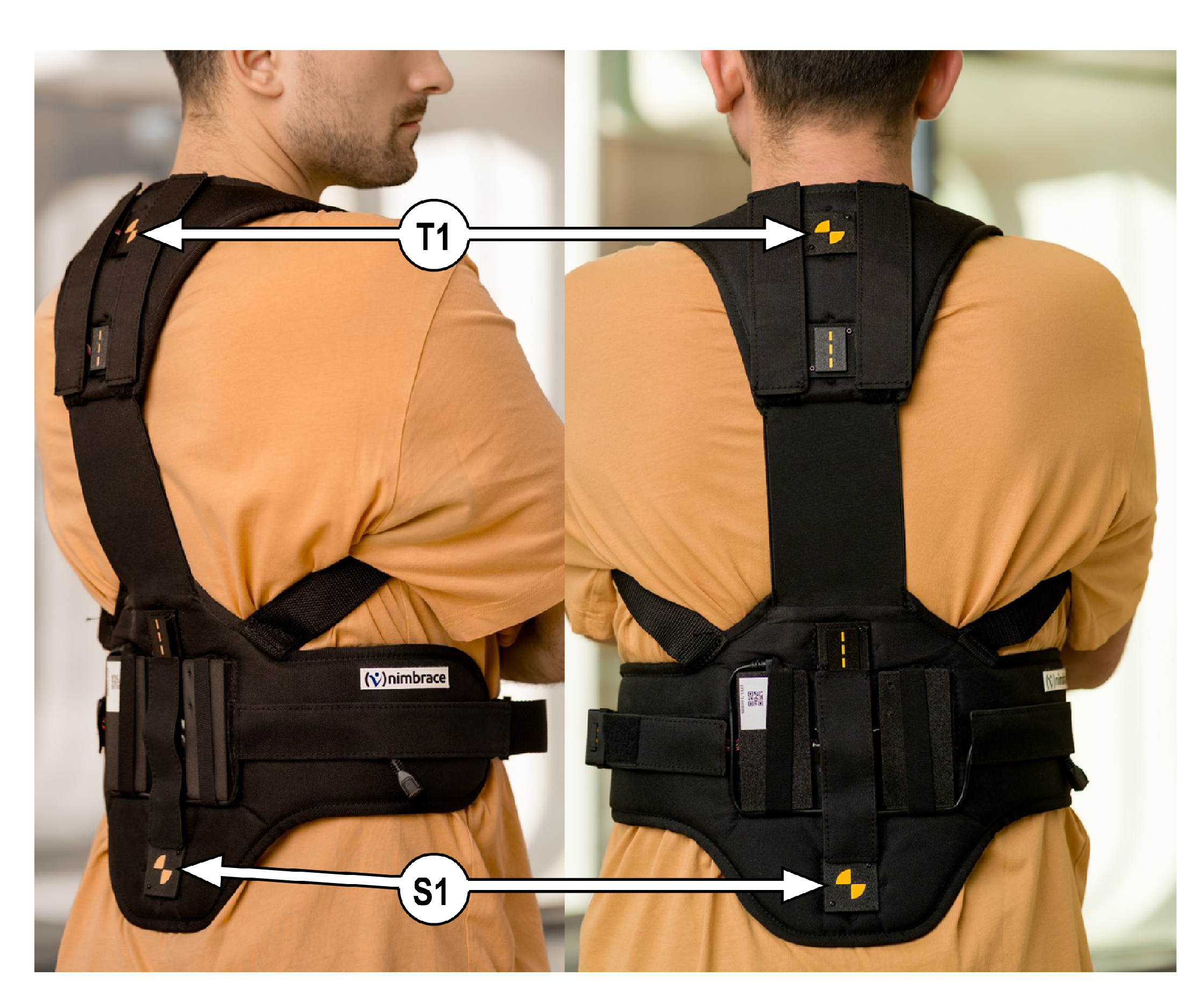
Figure 2.
Per-cycle stream for the index patient (Z) across recording days. Each panel is one complete day of monitoring, with all of that day’s recording files concatenated in order, and the panels run from the pre-treatment baseline through the post-injection course. For every gait cycle, the within-cycle excursion from neutral (peak, red) and the return position—the distance of the cycle’s return from the local neutral (valley, blue)—are plotted against cycle count. Each day contains several hundred to several thousand cycles. Display units are degrees of differential trunk–pelvis orientation.
Figure 2.
Per-cycle stream for the index patient (Z) across recording days. Each panel is one complete day of monitoring, with all of that day’s recording files concatenated in order, and the panels run from the pre-treatment baseline through the post-injection course. For every gait cycle, the within-cycle excursion from neutral (peak, red) and the return position—the distance of the cycle’s return from the local neutral (valley, blue)—are plotted against cycle count. Each day contains several hundred to several thousand cycles. Display units are degrees of differential trunk–pelvis orientation.
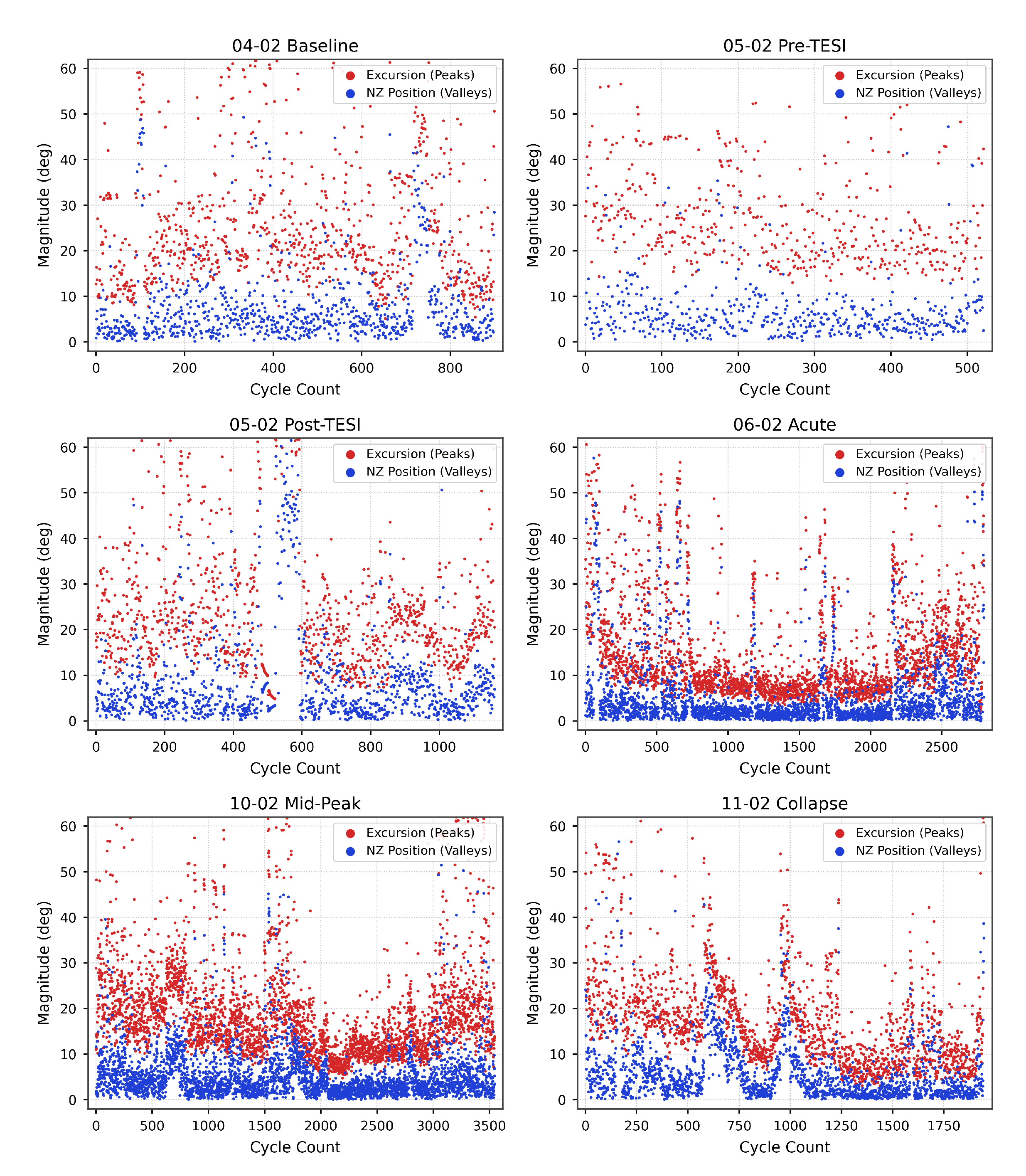
Figure 4.
Index patient (Z), T2-weighted lumbar MRI before treatment. Axial (left) and sagittal (right) images show lateral recess stenosis at the symptomatic level (arrowheads).
Figure 4.
Index patient (Z), T2-weighted lumbar MRI before treatment. Axial (left) and sagittal (right) images show lateral recess stenosis at the symptomatic level (arrowheads).
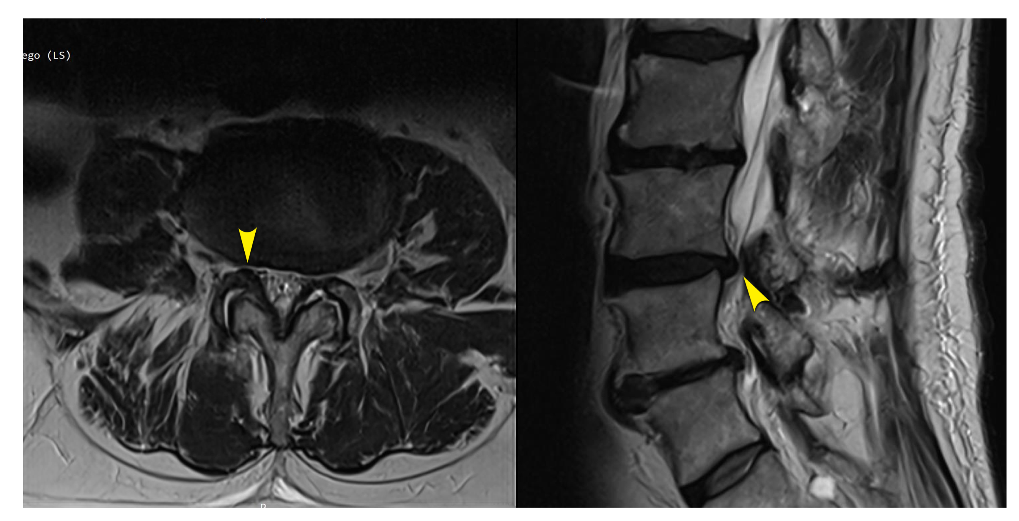

Table 1.
Per-patient pre-to-post effect on the per-cycle return metric, reported against each patient’s own plateau. Cliff’s delta is computed with the cycle as the unit of analysis; a positive value indicates a reduction of the metric after intervention.
Table 1.
Per-patient pre-to-post effect on the per-cycle return metric, reported against each patient’s own plateau. Cliff’s delta is computed with the cycle as the unit of analysis; a positive value indicates a reduction of the metric after intervention.
| Patient | Intervention | Cliff’s Delta | Per-Cycle Pattern |
|---|---|---|---|
| Z (index) | TESI | Return-metric collapse that held; late re-widening (see text) | |
| P | TESI | No shift; non-structural presentation. Within-study comparison case | |
| F | Foraminotomy | Collapse to a tight, low plateau held through follow-up | |
| K | Foraminotomy | Collapse with later partial re-widening; one mounting artefact flagged, not removed (conservative lower bound) |
Table 2.
Patient-reported outcomes at the first and last day of each monitoring period, with the corresponding per-cycle effect size from Table 1. ODI, Oswestry Disability Index; COMI, Core Outcome Measures Index.
Table 2.
Patient-reported outcomes at the first and last day of each monitoring period, with the corresponding per-cycle effect size from Table 1. ODI, Oswestry Disability Index; COMI, Core Outcome Measures Index.
| Patient | ODI (%) | COMI (/10) | Cliff’s Delta | Agreement |
|---|---|---|---|---|
| Z (index) | Concordant | |||
| K | Concordant | |||
| F | Concordant | |||
| P | Discordant |
Disclaimer/Publisher’s Note: The statements, opinions and data contained in all publications are solely those of the individual author(s) and contributor(s) and not of MDPI and/or the editor(s). MDPI and/or the editor(s) disclaim responsibility for any injury to people or property resulting from any ideas, methods, instructions or products referred to in the content. |
© 2026 by the authors. Licensee MDPI, Basel, Switzerland. This article is an open access article distributed under the terms and conditions of the Creative Commons Attribution (CC BY) license (http://creativecommons.org/licenses/by/4.0/).
Copyright: This open access article is published under a Creative Commons CC BY 4.0 license, which permit the free download, distribution, and reuse, provided that the author and preprint are cited in any reuse.