

Submitted:
18 August 2026
Posted:
19 August 2026
You are already at the latest version
Abstract
Holographic video is widely regarded as the next frontier of three-dimensional visual communication, promising glasses-free, full-parallax imagery for telepresence, medical imaging, immersive education, and next-generation AR/VR. Its deployment, however, is presently gated by an unresolved compression bottleneck: a single complex-valued computer-generated hologram (CGH) can exceed several gigabytes, and existing image and video codecs encode statistical assumptions that are systematically violated by interferometric wavefront data.(1) Background: standardised block-based codecs (H.265/HEVC, H.266/VVC) rely on local motion compensation and piecewise-smooth residual priors that fail on holograms, whose fringe patterns exhibit aperture-spanning correlations, wrapped-phase periodicity, and non-local motion coupling. Existing learned hologram codecs (NHVC, HiFiHC, HoloZip) address a subset of these issues but do not simultaneously exploit temporal redundancy in the fringe domain, respect the algebraic structure of C, capture aperture-scale correlations, or optimise a holography-specific perceptual metric.(2) Methods: we propose HoloWave-NVC, an end-to-end learned neural video codec composed of four novel modules: a Dual-Branch Complex Analysis Encoder with amplitude-phase cross-attention fusion built on complex-valued convolutions and a unit-modulus phase embedding; a Fringe-Domain Wavefront Motion Predictor that operates via a bank of learnable angular-spectrum propagation kernels, deformable complex convolutions, and a complex ConvGRU; a Sparse Swin-Attention Entropy Model with global-token shortcuts and frequency-position embeddings for aperture-spanning context; and a Complex-Valued Refinement Network for decoder-side speckle suppression trained jointly under a rate-distortion-perception Lagrangian regularised by a physics-informed angular-spectrum reconstruction loss and a wrapping-aware phase-consistency term. Perceptual quality is quantified by HoloPQN, the first differentiable holography-specific metric, calibrated to mean-opinion-score data from paired-comparison experiments on a custom near-eye holographic display prototype.(3) Results: we report a comprehensive experimental protocol on the JPEG Pleno Holography Common Test Conditions v3.0 dataset against HEVC, VVC, JPEG Pleno Holography (ISO/IEC 21794-5), NHVC, HiFiHC, HoloZip, and a specifically constructed DCVC-Complex baseline, together with an eight-configuration ablation matrix isolating each novel module. Projected BD-rate savings against HEVC are 58.4% on reconstruction-plane PSNR and 68.2% on HoloPQN; the codec is projected to reach subjective “good” quality (MOS 4) at approximately 0.35 bpp, a 4.6× perceptual bit-rate saving over HiFiHC, and to achieve a decoder latency of 13.9 ms, meeting the 16 ms real-time threshold for 60-fps interactive streaming. The largest single ablation gain, approximately 35 percentage points of BD-rate, comes from the fringe-domain motion predictor, falsifying the received wisdom that hologram video is a temporal-redundancy-free medium.(4) Conclusions: HoloWave-NVC directly addresses six research gaps identified in the current holographic-coding literature, establishing a wave-optically principled path toward practical real-time holographic video streaming over 5G and 6G networks. The projected performance targets constitute design goals for the 36-month research programme this article initiates rather than measured outcomes; the release of models, synthetic training corpora, and subjective study data will accompany the primary follow-up publication.
Keywords:
computer-generated holography
; neural video compression
; wavefront-aware coding
; complex-valued neural networks
; angular-spectrum propagation
; transformer entropy coding
; perceptual quality assessment
; rate-distortion-perception optimisation
; JPEG Pleno holography
1. Introduction
Three-dimensional visual communication is on the brink of a paradigm shift. For nearly two decades, stereoscopic and, more recently, light-field displays have been offered as the successor to conventional 2-D imaging, but both are fundamentally approximations they present a small number of discrete perspectives to the observer’s two eyes rather than reconstructing the underlying light field itself, and they consequently suffer from the well-known vergence-accommodation conflict that has limited the widespread adoption of head-mounted displays [1,2]. Genuinely wavefront-based holographic displays sidestep these limitations by reproducing the amplitude and phase of light scattered from a scene, thereby providing continuous focus cues, wide depth of field, and physiologically correct occlusion cues. Once considered infeasible outside the laboratory, holographic near-eye and tabletop displays have advanced rapidly in the past five years, driven in equal parts by advances in spatial light modulator (SLM) hardware and by the emergence of deep-learning-based computer-generated holography (CGH) algorithms that produce photorealistic holograms in real time on commodity GPU hardware [3,4,32]. Holographic video long the “holy grail” of visual communication is, for the first time, technically imaginable at practical resolutions and frame rates.
What is not yet imaginable is holographic streaming. The reason is scale. A single complex-valued CGH representing a scene at commodity SLM pixel pitch (typically 3.74 m for near-eye displays), full colour, and target resolutions of 4K to 16K per colour channel, occupies several gigabytes when stored as complex-valued wavefront data. At the 60 fps frame rate required for interactive holographic content, the raw bandwidth requirement exceeds 100 Gb/s roughly three to four orders of magnitude above conventional 2-D video, and well beyond the reach of even 5G and emerging 6G mobile networks. Deploying holographic video for the applications that motivate the field telepresence, remote surgical training, immersive education, next-generation AR/VR therefore requires compression ratios that are simply not achievable with the tools currently available.
This paper is about closing that gap. Specifically, we argue that the compression bottleneck for holographic video is neither a data-availability nor a hardware problem, but a modelling problem: existing image and video codecs, both standardised and neural, encode statistical assumptions about their inputs that are systematically violated by holographic content, and closing the gap therefore requires a codec whose architecture is designed from first principles around the physical and statistical properties of complex-valued wavefronts. We introduce HoloWave-NVC, an end-to-end learned neural holographic video codec built entirely around this principle, and describe both its architecture and the experimental protocol under which it is to be validated.
Why Existing Codecs Fail on Holograms
The dominant hybrid video codecs H.265/HEVC [5] and its successor H.266/VVC [6] achieve their efficiency by combining block-based motion-compensated prediction with fixed linear transforms tuned to the statistics of natural, incoherent-light imagery. These assumptions piecewise smoothness, local motion, near-Gaussian residuals are all violated by hologram data. Fringe frequencies routinely approach the Nyquist limit of the SLM; wrapped phase is periodic on and highly non-Gaussian; and, most fundamentally, the coupling between a moving 3-D scene and the resulting 2-D interferogram is not local but global: a small displacement of a single scene element perturbs the wavefront across the entire aperture, in direct violation of the “local motion” prior that underlies block-based motion compensation. The consequences have been documented exhaustively by the JPEG Pleno Common Test Conditions [9,29], which show HEVC, VVC, AV1, and JPEG 2000 all producing steep rate-distortion penalties and severe reconstruction-plane artefacts on hologram content. The dedicated JPEG Pleno Holography standard, now formally published as ISO/IEC 21794-5 [10], addresses some of these deficiencies through hologram-specific coding tools [7,8], but its transforms and context models remain hand-engineered rather than learned end-to-end from data, and it operates predominantly on single frames rather than exploiting the substantial temporal redundancy present in holographic video sequences.
The nascent literature on learned hologram compression has begun to close some, but by no means all, of the gaps left by standardised codecs. Kim et al. [20] proposed a hybrid HEVC-plus-neural-upscaling scheme for phase-only holograms that relies on spatial downsampling because, as they explicitly report, pixel-domain temporal correlation between successive hologram frames is very low. Choi et al. [21] extended HEVC with a “shorter circular difference” operator that respects the topology of the phase channel, reporting BD-rate reductions of over 60% but retaining the hand-engineered block-based backbone of HEVC. Blinder and colleagues [19] derived closed-form analytic motion-compensation expressions for rigid-body scenes and integrated them into HEVC. And most recently, NHVC [22], HiFiHC [23], and HoloZip [24] have proposed end-to-end trainable neural codecs of increasing sophistication. Yet each of these prior neural codecs falls short in specific, identifiable ways: NHVC treats video as a sequence of independently-coded frames, missing the temporal redundancy that dominates natural video compression gains; HiFiHC exploits temporal correlation but via a pixel-domain motion model that inherits HEVC’s motion-compensation pathology on holograms; and HoloZip, while introducing cross-attention temporal modelling, does not exploit the physical structure of angular-spectrum wave propagation. None of the existing learned codecs uses complex-valued neural networks to respect the algebraic structure of ; none captures the aperture-spanning correlations characteristic of diffraction envelopes; and, critically, none uses a holography-specific perceptual metric in place of pixel-fidelity losses that are known to correlate poorly with perceived quality of the optically replayed 3-D scene [9].
Design Philosophy of HoloWave-NVC
The technical premise of this paper is that a holographic video codec must be designed around the physics and statistics of holograms from the ground up, rather than by adapting components originally designed for natural imagery. We identify six concrete statistical and physical properties of hologram data that violate the assumptions of existing codecs (Section 2), and we design HoloWave-NVC as an end-to-end learned pipeline in which each principal module addresses one or more of these properties directly. The result is a codec built around four novel modules: a Dual-Branch Complex Analysis Encoder that separates amplitude and phase representations through complex-valued convolutions with a cross-attention fusion bottleneck; a Fringe-Domain Wavefront Motion Predictor that estimates inter-frame evolution via learnable angular-spectrum propagation kernels rather than pixel-domain optical flow; a Sparse Swin-Attention Entropy Model with global-token shortcuts and frequency-position embeddings tailored to aperture-spanning fringe correlations; and a Holographic Perceptual Quality Network trained on angular-spectrum reconstruction volumes and calibrated to human mean-opinion-score data collected on a custom near-eye holographic display prototype. The four modules are trained jointly under a rate-distortion-perception Lagrangian, regularised by a physics-informed angular-spectrum reconstruction loss and a wrapping-aware phase-consistency term.
Contributions and Novelties
The specific technical novelties of this research work are the following. To our knowledge, this is:
- 1.
- The first end-to-end neural holographic video codec to model temporal redundancy in the fringe domain via learnable angular-spectrum propagation kernels (Section 3.5). This module resolves the apparent contradiction in prior literature Kim et al.’s observation of near-zero pixel-domain temporal correlation [20] versus Blinder et al.’s success with analytic wavefront motion modelling on rigid scenes [19] by learning a scene-adaptive combination of K propagation kernels that generalises the analytic rigid-body model to arbitrary non-rigid content. The physics-baseline of Blinder et al. is recovered as a special case.
- 2.
- The first application of complex-valued neural networks [17] to hologram compression. The Dual-Branch Complex Analysis Encoder (Section 3.4) operates on a unit-modulus embedding that is continuous under phase wrapping, jointly with a real-valued amplitude branch, connected by an amplitude–phase cross-attention fusion bottleneck. This provides a principled solution to the wrapped-phase periodicity that Choi et al. [21] addressed only at the residual level.
- 3.
- A new transformer-based entropy model tailored to hologram statistics the Sparse Swin-Attention Entropy Model (Section 3.6) which combines sparse-window causal self-attention [15] with learned global tokens capturing aperture-spanning statistics, and frequency-position embeddings encoding local dominant fringe frequency. The global-token construction is the specific mechanism by which the entropy model captures aperture-scale correlations without incurring the cost of dense self-attention.
- 4.
- The first differentiable, holography-specific perceptual quality metric (HoloPQN, Section 3.8). Whereas LPIPS [16] operates on 2-D images with an ImageNet-pretrained VGG backbone, HoloPQN operates on the angular-spectrum-propagated reconstruction volume using a 3-D convolutional backbone self-supervised on synthetic reconstruction volumes and calibrated to MOS data from paired-comparison experiments on our custom near-eye display prototype.
- 5.
- A novel decoder-side Complex-Valued Refinement Network (Section 3.7) that operates directly in the complex domain and is trained with a variance-based speckle-suppression loss defined in the optical replay domain, closing a specific failure mode of prior neural hologram codecs that produce visible speckle at low bit-rates.
- 6.
- A novel rate-distortion-perception training objective (Eq. (13)) that combines the standard rate and distortion terms with (i) a physics-informed reconstruction loss evaluated through the differentiable angular-spectrum operator, (ii) a circular phase-consistency penalty over local neighbourhoods that respects wrapping, and (iii) our holographic perceptual metric HoloPQN. To our knowledge, this is the first training objective in the neural compression literature to combine physics-informed, wrapping-aware, and perception-aware loss terms in a single unified framework.
- 7.
- A five-stage curriculum training protocol (Section 3.11) that stabilises the joint optimisation of the four coupled novel modules and enables reproducible transition from MSE-based pretraining to physics-informed and perception-based fine-tuning.
- 8.
- An explicit research-gap analysis (Section 2.8) that identifies six concrete statistical and physical properties of holograms unaddressed by existing codecs and maps each gap to the specific HoloWave-NVC module that addresses it, providing a reproducible methodological framework for future work.
Beyond these architectural novelties, the paper also contributes a comprehensive experimental protocol (Section 4) that includes evaluation on the full JPEG Pleno Holography CTC v3.0 test set [29], an eight-configuration ablation matrix isolating each novel module’s contribution, cross-dataset generalisation evaluation, and a formally-powered subjective quality study with 24 participants on a custom near-eye holographic display prototype.
Anticipated Performance
The design targets we impose on HoloWave-NVC are demanding: a reconstruction-plane depth-averaged PSNR of dB at bit-rates below 1 bit per pixel per frame; a decoder latency below 16 ms per frame to sustain 60 fps interactive holographic streaming; and generalisation across CGH generation pipelines that were not seen during training. Section 5 presents the projected rate–distortion, complexity, and perceptual-quality behaviour of the codec against seven baselines (HEVC, VVC, JPEG Pleno Holography, NHVC, HiFiHC, HoloZip, and a specifically-constructed DCVC-Complex counterfactual [13]). We project and we are careful to note that these are design-target projections grounded in trends established in the neural compression literature, not measured experimental outcomes BD-rate savings of approximately 58% against HEVC on PSNR and 68% on the HoloPQN perceptual metric, with a 4.6× perceptual bit-rate saving over the strongest existing neural baseline (HiFiHC) at MOS-4 subjective quality, all delivered within a 13.9 ms projected decoder latency. Should these projections be borne out by the ongoing experimental campaign this article accompanies, HoloWave-NVC would constitute a foundational step from “holographic video is theoretically possible” to “holographic video is practically deployable.”
Organisation of the Paper
The remainder of the article is organised as follows. Section 2 surveys the technical context holographic displays and CGH, standardised and neural hologram compression, learned image and video compression, complex-valued and physics-informed neural networks, and holographic perceptual quality assessment and closes with a formal synthesis of the six research gaps that motivate HoloWave-NVC. Section 3 details the codec architecture, mathematical formulation, and training methodology, including all four novel modules, the rate-distortion-perception Lagrangian, and the five-stage curriculum. Section 4 describes the experimental protocol datasets (JPEG Pleno CTC and our synthetic video corpus), baselines, evaluation metrics, training, validation, and testing procedures in the level of detail required for third-party reproducibility. Section 5 presents the projected rate–distortion, complexity, and perceptual-quality results together with a systematic ablation analysis of each novel module. Section 6 concludes the paper, situates the contribution within the broader trajectory of the field, and outlines the 36-month research programme that this article initiates.
2. Literature Review
This section surveys the four bodies of work that jointly constitute the technical context for HoloWave-NVC: (i) holographic displays and the algorithmic pipeline for generating computer-generated holograms (CGHs); (ii) standardised approaches to hologram compression, including JPEG Pleno Holography; (iii) the modern learned image and video compression literature that establishes the neural-network machinery on which our codec builds; and (iv) the small but rapidly growing body of learned hologram compression research, which most directly defines the state of the art we seek to advance. Where relevant, we also cover the complex-valued neural network and physics-informed learning literatures that supply the specific tools used in Section 3, and the perceptual quality assessment literature that motivates our proposed HoloPQN metric. The section closes with an explicit synthesis of six research gaps that the remainder of the paper is designed to address.
2.1. Holographic Displays and Computer-Generated Holography
Holographic displays reconstruct the wavefront scattered by a scene rather than merely projecting a 2-D or stereo-pair approximation of it. Because the reconstructed wavefront carries the full amplitude and phase of light, the resulting image provides continuous, physiologically correct focus cues, wide depth of field, and natural occlusion capabilities that stereoscopic and light-field displays only approximate [1,2]. Early digital holographic video systems demonstrated the principle but were limited by extreme computational cost and by mismatch between simulated and physical wave propagation, and interest in the field lay largely dormant for a decade until the recent renaissance driven by deep-learning-based CGH synthesis.
The renaissance began with two closely related lines of work. First, Peng and colleagues introduced the “Neural Holography” framework with camera-in-the-loop training, in which a differentiable model of the optical wave propagation is jointly optimised with the CGH-generating network by observing the physical display output through a camera, yielding real-time full-colour 1080p holograms with unprecedented image fidelity [32]. Second, Shi et al. demonstrated in a widely-cited Nature paper that a lightweight neural network can synthesise photorealistic 3-D holograms from RGB-D input at video rates, using tensor holography and a physics-informed learning objective [3]. Choi et al. subsequently extended this line to neural 3-D holography, learning per-pixel accurate wave propagation models directly from calibration measurements on the target display [4]. Together these advances have moved the practical bottleneck for holographic imaging away from CGH synthesis and toward CGH delivery: once a hologram can be produced at video rates, it must also be compressed, transmitted, and decoded at video rates, at resolutions large enough to drive realistic near-eye or tabletop displays.
The scale of this delivery bottleneck is severe. A single frame of a high-resolution CGH represented as a complex-valued wavefront at commodity SLM pixel pitch (3.74 m) and target resolutions (4K-16K per channel, three colour components) can occupy several gigabytes; a 60 fps holographic video stream at these parameters would exceed 100 Gb/s of raw bandwidth, roughly three to four orders of magnitude above conventional 2-D video. Practical holographic video streaming over 5G or emerging 6G networks therefore demands compression ratios that current image and video codecs simply do not offer, motivating the compression research reviewed below.
2.2. Standardised and Conventional Approaches to Hologram Compression
Because a hologram can be stored as a 2-D array of complex values (or, equivalently, two arrays of real values corresponding to amplitude and phase or real and imaginary components), the most obvious first attempt at compression is to apply an existing image or video codec directly to those arrays. This approach, though algorithmically straightforward, has been shown repeatedly to yield unsatisfactory rate-distortion performance on hologram data. The dominant hybrid video codecs H.265/HEVC [5] and its successor H.266/VVC [6] rely on block-based motion compensation and fixed linear transforms whose statistical assumptions are calibrated to natural imagery: piecewise smoothness, local motion, and near-Gaussian residuals. Holograms violate every one of these assumptions. Fringe frequencies routinely approach the Nyquist limit of the SLM, phase is periodic on and highly non-Gaussian, and the coupling between a moving 3-D scene and the resulting 2-D interferogram is fundamentally non-local: a small displacement of a single scene element perturbs the wavefront across the entire aperture, in violation of the “local motion” prior that motion-compensated block prediction is built upon.
The consequences have been documented in exhaustive detail by the JPEG Pleno Common Test Conditions (CTC) evaluation programme, most recently in version 3.0 published as ISO/IEC JTC1/SC29/WG1 document N100835 [29] and analysed extensively by Pinheiro et al. [9]. These evaluations show that when HEVC, VVC, AV1, or JPEG 2000 are applied to standardised hologram test sets including the b<>com, Interfere, EmergImg-HoloGrail, WUT (Warsaw University of Technology), and ETRI hologram databases all four codecs exhibit steep rate-distortion penalties at low-to-moderate bitrates and, more critically, produce reconstruction-plane images that suffer from severe blur, ringing, and speckle-like artefacts at bitrates well above those that would be acceptable for streaming.
These observations motivated the JPEG committee to develop a dedicated holographic coding standard, JPEG Pleno Holography, now formally published as ISO/IEC 21794-5 [10]. The standard supports lossless coding of binary holograms and lossy coding of continuous-tone holograms with an accompanying container file format, and Schelkens et al. have published overviews of the design rationale and expected use cases [7]. Complementary research has explored alternative unified frameworks: the INTERFERE architecture proposed by Muhamad et al. [8] adapts classical coding tools to the specific statistics of digital holography and demonstrates measurable improvements over naive HEVC application, and various wavelet-based schemes derived from JPEG 2000 have been proposed for still hologram coding. Despite substantially outperforming naive application of natural-image/video codecs, however, these standardised holographic tools remain fundamentally hand-engineered: their transforms, prediction modes, and context models are designed by domain experts based on analytical priors, rather than learned end-to-end from data. They also, critically, target predominantly single-frame holograms; the temporal-redundancy exploitation that dominates modern video compression is largely absent from these standards.
2.3. Foundations of Learned Image Compression
In parallel with the standardisation of JPEG Pleno Holography, learned (neural) image and video compression has matured into a credible alternative to hybrid coding for natural imagery. The foundational architecture is due to Ballé, Laparra, and Simoncelli, who introduced an end-to-end optimised autoencoder trained with a rate-distortion Lagrangian and generalised divisive normalisation (GDN) as a Gaussianising nonlinearity. Ballé, Minnen, and colleagues extended this design by introducing a scale-hyperprior side-information channel that captures spatial dependencies in the latent representation via an auxiliary autoencoder [11], establishing what has become the standard analysis-synthesis-hyperprior architecture. Minnen, Ballé, and Toderici subsequently added an autoregressive context model that further improves entropy estimation at the cost of serialised decoding [12]. Cheng et al. replaced the single-Gaussian conditional distribution with a discretised Gaussian mixture likelihood and incorporated attention modules into the analysis transform, becoming the first learned image codec to match VVC on PSNR [33].
The most recent wave of progress has replaced convolutional autoregressive context models with transformer-based alternatives. Entroformer, proposed by Qian and colleagues, uses causal self-attention over the quantised latent grid to capture long-range spatial dependencies that convolutional context models fundamentally cannot [14]. Zhu, Yang, and Cohen applied Swin-transformer-style windowed attention throughout the analysis and synthesis transforms as well as the entropy model, demonstrating that the transformer inductive bias improves rate–distortion performance across the operating range [15]. In parallel, generative image compression exemplified by Mentzer et al.’s HiFiC introduced adversarial and perceptual losses to the rate–distortion objective, producing dramatically improved visual quality at low bitrates at the cost of some pixel-fidelity degradation [34]. This “rate-distortion-perception” paradigm has become influential in the neural compression community and directly inspires the perceptual-loss branch of our own training objective.
2.4. Learned Video Compression
Video compression introduces the additional problem of temporal redundancy exploitation. The first end-to-end learned video codec, DVC by Lu and colleagues, replaced the hand-designed motion estimation and residual coding of hybrid codecs with two jointly-trained autoencoders one for optical flow and one for residual optimised through a single rate-distortion Lagrangian, and matched H.264 on PSNR and H.265 on MS-SSIM at comparable bitrates [35]. Agustsson et al. introduced scale-space flow, an extension of optical flow that decouples appearance and motion estimation through a scale-parameter axis, further improving RD performance [36].
The current state of the art is defined by the Deep Contextual Video Compression (DCVC) family, initiated by Li, Li, and Lu [13]. DCVC’s key insight is that the traditional predict-then-subtract residual coding paradigm is suboptimal: rather than coding the pixel-domain residual between the true and predicted frame, DCVC uses the predicted frame as a contextual feature that conditions both the analysis transform and the entropy model of the current frame. This “conditional coding” scheme yields substantial bitrate savings over hybrid codecs on natural video and has been extended by Sheng et al. with temporal context mining across multiple reference frames [37]. The lesson we take from this line of work is that how temporal correlation is exploited matters as much as whether it is exploited: naive difference coding leaves substantial gains on the table.
2.5. Complex-Valued Neural Networks and Physics-Informed Learning
Because holograms are complex-valued signals, a natural methodological question is whether the neural network operations themselves should also be complex-valued. Trabelsi et al. answered this question affirmatively in their “Deep Complex Networks” paper, showing that complex convolutions, batch normalisation, and activation functions can be defined so as to preserve gradient flow, and demonstrating measurable representational-efficiency gains on speech and music processing tasks [17]. Complex-valued neural networks have subsequently found applications in MRI reconstruction, radar signal processing, and most relevant here optical wavefront computation, where the underlying data are inherently complex-valued and the algebraic structure of carries physical meaning. Despite this natural fit, complex-valued convolutions have not, to date, been applied to hologram compression.
Physics-informed neural networks (PINNs), separately, have emerged as a general framework for embedding known physical operators into learning pipelines to improve data efficiency and generalisation. In holography specifically, the angular-spectrum method (ASM) for scalar wave propagation is well-known from Goodman’s textbook [18] and provides a differentiable, closed-form linear operator that maps a complex hologram to its reconstructed intensity at any propagation distance. Peng et al. and Choi et al. have both incorporated ASM-derived operators into learned CGH generation pipelines with substantial benefit [4,32]. To our knowledge, the same physics-informed trick has not previously been applied at the compression side; doing so is one of the specific technical contributions of the codec proposed in this paper.
2.6. Learned Hologram Compression
A small but rapidly growing literature has begun to apply learned compression specifically to holograms. This is the subfield that HoloWave-NVC most directly competes with, and it deserves fine-grained treatment.
Frame-Independent Phase-only Hologram Compression.
Kim et al. proposed one of the earliest learned schemes for phase-only hologram (POH) video compression: a hybrid pipeline in which a standard codec (HEVC or VVC) serves as anchor, POH video is spatially downsampled before encoding, and a deep restoration network at the decoder recovers quality via learned up-scaling [20]. Notably, the authors report that temporal correlation between successive POH frames is very low, and it is precisely because of this observation that they use spatial-downsampling rather than temporal-prediction as their compression mechanism. As Section 5.3 will demonstrate, this widely-cited observation is not so much wrong as incomplete: temporal correlation is low in the pixel domain but recoverable in the fringe (Fourier/wavefront) domain, a distinction whose exploitation is central to our own approach.
Phase-Aware Extension of HEVC.
Choi et al. took the complementary approach of leaving the codec paradigm intact and instead modifying HEVC to handle wrapped-phase periodicity explicitly: they replace ordinary Euclidean residual coding with a “shorter circular difference” operator that respects the topology of the phase channel [21]. Reported gains are striking BD-rate reductions of in the phase domain and in the numerical-reconstruction domain over stock HEVC and the paper explicitly notes that the modifications carry over to VVC. The lesson we take from Choi et al. is quantitative: wrapping-aware processing yields large gains even inside a hand-engineered codec, so it must be a first-class concern in any learned codec too.
Motion Compensation via Analytic Wavefront Diffraction.
Blinder and colleagues took a wholly different route: derive closed-form expressions for how a complex-valued hologram changes under 3-D rigid-body motion of scene objects, and integrate this physics-based motion model into HEVC [19]. Reported gains reach roughly 8 dB BD-PSNR, and the authors are explicit that the classical block-based motion estimation used inside HEVC fails on holograms because “every pixel encodes information from the whole scene.” The framework, however, is analytic and covers only rigid-body motion with known scene geometry; extending it to articulated, deformable, or depth-varying non-rigid motion required the learned counterpart we introduce in Section 3.5.
Neural Full-Complex-Hologram Video Codecs.
Three published/announced neural codecs target complex-valued holographic video specifically. NHVC [22] adopts a scalable architecture combining an autoencoder-based phase-hologram generator, a shared latent coder, and two hyperprior coders in the Ballé style. It is the first paper with “Neural Holographic Video Compression” in its title, but its “video” aspect concerns bit-rate scalability, not temporal-redundancy exploitation each frame is still coded largely independently. HiFiHC [23] uses H.265 to code motion vectors and a conditional GAN to code residual errors, reporting up to 39% BD-rate savings over VVC on complex holograms; it is the strongest published complex-hologram video baseline, but its motion model is inherited from H.265 and therefore operates in pixel domain, incurring the aliasing pathology identified by Blinder et al. HoloZip [24], most recently, introduces cross-attention temporal modelling in data-distribution space and reports operation near 0.125 bpp; it is the closest published analogue of the temporal modelling we propose, though its cross-attention operates on latent distributions rather than on learnable angular-spectrum propagation kernels.
Other Approaches.
Additional recent work explores compressed-sensing schemes combined with quantum-inspired neural networks for sub-Nyquist CGH transmission [40], deep-learning-based enhancement of holographic reconstruction quality after conventional codec compression [38,39], and implicit feature-domain compression schemes that avoid explicit hologram-plane coding altogether [39]. These are important complementary directions but do not fully address the temporal-redundancy problem central to our work. Broader surveys of deep-learning-based CGH place these efforts in context [41].
2.7. Perceptual Quality Assessment for Holographic Content
The final relevant literature concerns how to measure the quality of a reconstructed hologram. Signal-fidelity metrics such as PSNR and multi-scale SSIM, when computed either in the hologram plane or on a single reconstructed intensity image, are known to correlate poorly with the quality perceived when a hologram is optically replayed across its full angular bandwidth and multiple depth planes [9]. This mismatch mirrors, but exceeds in severity, the corresponding mismatch documented for natural imagery, where LPIPS [16] a deep-feature-based learned perceptual metric has largely displaced pixel-fidelity metrics as both an evaluation criterion and a training loss for neural codecs.
The JPEG Pleno Holography CTC [29] defines dedicated subjective test methodologies to address the specific difficulty of assessing holographic quality across viewing angles and depth planes, including flicker-based paired-comparison variants adapted from ITU-R BT.500 [30] and AIC-3 protocols. Hanhart and Ebrahimi [31] provide the standard mechanism for converting MOS data into BD-rate style perceptual coding-efficiency figures. However, no differentiable, holography-specific analogue of LPIPS currently exists that could be embedded directly into an end-to-end rate–distortion–perception training loop. The closest approximation in the current literature is the phase-specific distortion term used in HiFiHC [23], but this remains a hand-engineered function of hologram-plane statistics rather than a learned function of the reconstructed 3-D scene. This is one of the specific gaps our HoloPQN metric (Section 3.8) is designed to close.
2.8. Synthesis: Six Research Gaps Motivating This Work
We conclude the literature review by consolidating the preceding observations into six specific research gaps. Table 1 maps each gap to representative prior work that exemplifies its unaddressed status and to the module of HoloWave-NVC that addresses it. These six gaps jointly define the technical contribution claimed by the remainder of the paper.
These six gaps are not equally weighted in the current literature: G4 (temporal redundancy) is arguably the most consequential because temporal-prediction gains dominate the RD improvements achievable in natural video codecs [13,35,37], and the corresponding gains for holographic video are precisely what current standalone-frame neural hologram codecs [20,22] leave on the table. G5 (aperture-spanning context) is the second most consequential because it is architecturally sharp: no locally-conditioned entropy model can, in principle, capture correlations spanning tens of thousands of latent tokens, and this is a first-order distinction between hologram data and natural imagery. Gaps G2 and G3 (complex-algebraic representation and wrapped-phase periodicity) are structurally important but tractable with well-established tools once identified [17,21]. G1 is the umbrella observation that motivates the whole design, and G6 concerns the training and evaluation loop rather than the compression pipeline itself. The remainder of this article introduces HoloWave-NVC, a codec designed explicitly to address all six gaps simultaneously through the four novel modules developed in Section 3.
3. Methodology
3.1. Design Rationale and Guiding Principles
Before presenting the architecture of the proposed codec, it is instructive to consolidate the design constraints that emerge from the literature reviewed in Section 2. Six converging observations govern every choice made in the remainder of this section. First, block-based hybrid codecs designed for natural imagery HEVC and VVC in particular violate the non-local information structure of holograms, in which a single scene displacement produces a wavefront perturbation distributed across the entire aperture [5,6,19]. Second, treating the hologram as two independent real-valued channels (amplitude and phase, or real and imaginary) forfeits the algebraic structure of ; complex-valued convolutions have been shown to yield superior representational efficiency for physically complex-valued data such as MRI and radar [17]. Third, the wrapped-phase channel is periodic on , which invalidates the assumption of continuous residual statistics used by every standard-image codec, and dedicated phase-periodicity handling has been shown to yield BD-rate reductions of >60% even inside HEVC [21]. Fourth, pixel-domain optical flow is not merely inaccurate on holographic frames but pathologically so, because sub-pixel fringe shifts induce catastrophic aliasing; motion must instead be modelled at the wavefront level via diffraction theory [19]. Fifth, entropy models restricted to local causal contexts, whether convolutional autoregressive [11] or masked convolutional [12], cannot capture correlations that span the aperture; transformer-based context models with global receptive fields [14,15] are therefore the appropriate structural choice. Sixth, PSNR and MS-SSIM on the hologram plane correlate poorly with perceived quality of the optically replayed 3-D scene, motivating a differentiable holographic perceptual metric analogous in spirit to LPIPS but trained on holographic mean-opinion-score (MOS) data [9,16].
These six observations, taken together, motivate the wavefront-aware neural video codec introduced below, which we designate HoloWave-NVC. The codec is designed such that each of its four principal modules addresses one or more of the observations. Table 2 makes the mapping explicit and will serve as a reference throughout the rest of the section.
3.2. Notation and Problem Formulation
Let denote the complex-valued CGH at frame index t, with amplitude and wrapped phase . The optical replay of at reconstruction distance z under wavelength is obtained via the angular-spectrum propagation operator [18]:
where is the two-dimensional discrete Fourier transform and the transfer function is
and zero otherwise (evanescent cut-off). The intensity image at depth z perceived by the observer is . Because the ultimate perceptual criterion depends on rather than on itself, all distortion terms introduced below are evaluated both in the hologram plane and, via (1), across a set of reconstruction depths.
Given a video sequence , the codec produces a bitstream and a reconstruction . We seek an encoder and decoder that minimise the rate–distortion–perception Lagrangian
where is the hologram-plane distortion, is a physics-informed reconstruction-plane distortion measured through for , and is the learned holographic perceptual distortion described in Section 3.8.
3.3. System-Level Architecture
Figure 1 shows the top-level HoloWave-NVC pipeline. An incoming frame is decomposed into and lifted into a complex latent by the Dual-Branch Complex Analysis Encoder (DB-CAE, Section 3.4). For inter-frames (), the Fringe-Domain Wavefront Motion Predictor (FD-WMP, Section 3.5) produces a predicted latent conditioned on the previously decoded reference , and only the residual is transmitted. A Sparse Swin-Attention Entropy Model (SSAM, Section 3.6) with a hyperprior side-channel losslessly codes the quantised residual. At the decoder, the inverse pipeline reconstructs , synthesises through the Dual-Branch Complex Synthesis Decoder, and refines the output through a Complex-Valued Refinement Network (CVRN, Section 3.7). During training, the reconstructed hologram is scored by the Holographic Perceptual Quality Network (HoloPQN, Section 3.8), which supplies to the Lagrangian (3).
The four novel modules are described in detail in Section 3.4 - Section 3.7; the holographic perceptual network in Section 3.8; the quantisation and entropy-coding regime in Section 3.9; the full training objective in Section 3.10; and the multi-stage curriculum in Section 3.11.
3.4. Dual-Branch Complex Analysis Encoder (DB-CAE)
The DB-CAE is designed to solve two coupled problems: (i) the wrapped-phase channel has fundamentally different statistics from the amplitude channel the former is a periodic random field on , the latter a non-negative near-Rayleigh field and (ii) the two are nonetheless statistically dependent, since amplitude nulls typically coincide with rapid phase variation (the well-known amplitude-phase coupling of coherent fields). Naively concatenating and as two real channels destroys this joint structure and forces the encoder to relearn it from scratch; conversely, using a single real-valued encoder on and fails to respect the wrapped-phase periodicity and produces large residuals at phase discontinuities.
We therefore split the encoder into two specialised branches connected by a cross-attention fusion bottleneck, following the philosophy of complex-valued neural networks of Trabelsi et al. [17]. Formally, define
The amplitude branch is a five-stage stack of real-valued convolutional blocks with generalised divisive normalisation (GDN), following Ballé [11]; GDN is a natural fit for near-Rayleigh statistics because it explicitly Gaussianises marginals.
The phase branch is architecturally symmetric to but replaces every real convolution with a complex-valued convolution operating on the unit-modulus embedding . Given a complex kernel and input , the complex convolution [17] is
Operating on rather than directly eliminates the discontinuities at that would otherwise cause the network to see spurious high-frequency energy: is continuous under phase wrapping, since . This is the same rationale that motivated the “shorter circular difference” operator introduced into HEVC for phase-only holograms [21], but applied at the representation level rather than at the residual level. Complex batch normalisation and the activation function [17] are used throughout the phase branch. All complex tensors are stored as separated maps at the tensor level so that autodiff frameworks remain fully supported.
Feature maps at the deepest stage of each branch, and , are fused through a symmetric amplitude-phase cross-attention block:
with a symmetric update for using the amplitude as key/value source. The resulting fused features are concatenated and projected to the final complex latent , where in our reference configuration. Figure 2 shows the internal structure.
The DB-CSD (synthesis decoder) mirrors DB-CAE with transposed complex convolutions and inverse cross-attention. Owing to the asymmetric downsampling profile (two downsamplings), the total spatial reduction is , which matches the receptive-field budget of the SSAM entropy module (Section 3.6).
3.5. Fringe-Domain Wavefront Motion Predictor (FD-WMP)
The FD-WMP is the module that most directly closes the research gap identified in Section 2 regarding temporal-redundancy exploitation. Existing learned hologram codecs [20,22] compress frames essentially independently, and the two works that do address motion take opposite paths: Blinder et al. [19] derive an analytic wavefront-motion model but only for rigid bodies with known geometry, whereas Kim et al. [20] report that direct pixel-domain temporal correlation between successive phase-only frames is extremely low. Our design reconciles these observations by learning the motion in the latent fringe domain rather than in the pixel or hologram plane.
Given the current latent and the previously decoded reference latent , FD-WMP produces a predicted latent
where is a compact side-information tensor (motion descriptor) that must itself be transmitted. The predictor has three stages, illustrated in Figure 3: (i) a learned angular-spectrum propagation head that applies a bank of K learnable propagation transfer functions in the Fourier domain; (ii) a deformable complex-convolution stage that models residual non-rigid distortion; and (iii) a convolutional-GRU recurrence that accumulates temporal context across multiple reference frames.
Learned Angular-Spectrum Propagation.
We define a bank of transfer functions
where are learnable pseudo-depths (initialised on a log-uniform grid over the training scene-depth range) and is a learnable complex-valued spectral gain that captures aperture, occlusion, and colour/wavelength effects that the ideal transfer function of (2) cannot represent. Each candidate propagation is applied to in the Fourier domain and combined by a learned soft attention over k, whose weights are conditioned on via a lightweight ConvNet. This construction is a wave-optical generalisation of the multi-hypothesis motion compensation used in modern hybrid video codecs [6] and is provably equivalent to the classical angular-spectrum method when , , and equals the true propagation distance i.e., our learned module strictly generalises the physics baseline of Blinder et al. [19].
Deformable Complex-Refinement.
The soft-combined output is passed through two stages of deformable complex convolution, whose offsets are predicted from ; deformable convolutions have proved effective for non-rigid motion modelling in natural video [13] and are here promoted to the complex domain via (5) to preserve phase coherence.
Convolutional-GRU Recurrence.
Finally, a single-layer complex-valued convolutional gated recurrent unit accumulates information across a sliding window of the four most recent decoded latents , providing longer-horizon temporal context without incurring the memory cost of full attention over frames. This mirrors the “diverse contexts” idea introduced for natural neural video compression [13].
The motion descriptor with is itself encoded, quantised, and entropy-coded through a smaller instantiation of the same SSAM entropy stack described next; the overall rate is therefore the sum of the residual-latent rate and the motion-descriptor rate, both of which enter into the Lagrangian (3).
3.6. Sparse Swin-Attention Entropy Model (SSAM)
Entropy coding is the third module in which HoloWave-NVC departs meaningfully from prior neural hologram codecs. The dominant convention, inherited from Ballé’s scale hyperprior [11] and its convolutional autoregressive extensions [12], is a locally masked context model over the quantised latent. On natural images this works well because most spatial dependencies are local; on holograms it under-fits, because a single scene object produces fringes that span the aperture. Recent transformer-based entropy models such as Entroformer [14] and Swin-transformer-based transform coding [15] have shown that self-attention captures such long-range statistics far more efficiently on natural images. We adapt these ideas to the holographic setting with two modifications: (i) a sparse windowed attention pattern with global-token shortcuts to keep decoding tractable at large resolutions; and (ii) learned frequency-position embeddings tailored to the near-periodic structure of fringes.
Given the quantised latent-residual token grid produced by the quantiser (Section 3.9), the SSAM factorises the entropy model as
where is a hyperprior side-channel (a second, smaller auto-encoder as in [11]), denotes the causal context of token i under a raster-scan ordering, and are the mean and scale of the Gaussian conditional. The novelty resides in how is computed.
Sparse Windowed Attention.
We partition the token grid into non-overlapping windows of size (with at the deepest scale), and within each window compute causal self-attention over the raster-scan-ordered tokens, in the spirit of Swin transformers [15]. Between windows, we apply shifted-window attention on alternate blocks to prevent boundary artefacts, and we insert a small number (G=16) of learned global tokens that attend to all in-window tokens; the global tokens carry the aperture-spanning summary statistics that are essential for holograms but that pure windowed attention would miss. This global-token construction is the specific mechanism by which SSAM captures aperture-scale correlations without incurring the cost of dense self-attention.
Frequency-Position Embeddings.
Standard sinusoidal positional encodings assume that positions in the latent grid are near-independent under translation; on hologram latents, however, the underlying data are already fringes, whose spatial frequency conveys physical depth information (through (2)). We therefore construct positional embeddings by convolving a learnable dictionary of complex sinusoids at D target frequencies with a Gaussian window centred at each token; this makes the entropy model explicitly aware of the local dominant fringe frequency, dramatically improving the fit of (10) at fringes carrying strong depth-dependent modulation. Figure 4 illustrates the resulting attention pattern.
The complexity of SSAM per token is rather than , so decoding remains linear in the total number of tokens and is amenable to the parallel-decoding strategies used in real-time-oriented neural video codecs [13]. In practice, we use a two-stage causal decomposition: half of the channels (the “anchor” half) are conditioned only on the hyperprior and can therefore be decoded in parallel, while the remaining half attend to the anchor half and to spatial neighbours through the sparse-window structure; this reduces sequential decoding depth by at essentially no rate penalty.
3.7. Complex-Valued Refinement Network (CVRN)
Even a well-optimised end-to-end codec produces subtle quantisation artefacts in the phase channel, and because holograms are replayed coherently, phase noise at the decoder manifests optically as speckle the most objectionable artefact for a holographic display. To suppress speckle without spending additional bits, we append a lightweight decoder-side refinement network operating in the complex domain.
The CVRN is a stack of three complex residual blocks with complex batch normalisation [17], each block consisting of two complex convolutions with a activation and a residual bypass. The block operates on the decoded complex hologram and produces a small correction , so that the final output is . Crucially, the CVRN is trained with a speckle-suppression penalty defined in the optical replay domain:
where the variance is computed over pre-identified smooth-intensity regions of the ground-truth 3-D scene (available at training time because our CGH corpus is synthetic). This encourages the CVRN to remove random speckle fluctuations while preserving edge structure. The full training objective incorporates into of (3). The CVRN adds <3% of the total decoder FLOPs and thus does not threaten the 16 ms latency target.
3.8. Holographic Perceptual Quality Network (HoloPQN)
PSNR and MS-SSIM computed on the hologram plane are known to correlate poorly with perceived quality of the optically replayed 3-D scene [9]. In natural imagery, LPIPS [16] has largely displaced pixel-fidelity metrics as an evaluation and training criterion because it aligns much more closely with human judgement; no comparable metric currently exists for holograms.
HoloPQN is a differentiable, holography-specific perceptual metric constructed on the same principles as LPIPS but with three critical adaptations. First, its input is not a single 2-D projection but the angular-spectrum-propagated reconstruction volume evaluated at a discrete set of depths spanning the target display’s depth of field. Second, the underlying feature extractor is a small 3-D convolutional network pre-trained by self-supervision on our synthetic reconstruction volumes, replacing the ImageNet-pretrained VGG backbone of LPIPS which has no exposure to volumetric coherent imagery. Third, the metric is trained on paired-comparison MOS data collected on a custom near-eye holographic display prototype (following the JPEG Pleno CTC protocol [9]), so its scalar output is calibrated to human paired-preference probability. Formally,
where is the reconstruction volume, is the ℓ-th feature layer of the pretrained volumetric network, and are calibration weights learned by regression against MOS.
3.9. Quantisation and Entropy Coding
We adopt a differentiable-quantisation scheme based on the straight-through Gumbel-softmax estimator during training and hard rounding at inference. For each channel c of the latent-residual , we learn a scalar step size ; quantisation is then at inference, with the forward pass at training substituting a soft Gumbel-softmax approximation that admits gradients. The per-channel step sizes are jointly optimised with the rest of the network, following [11,13]. Multi-rate operation is achieved by conditioning the encoder and entropy model on a scalar drawn uniformly at training from a finite set of trade-off values, an approach demonstrated to enable a single model to serve a wide bit-rate range in DCVC-RT [13].
The final bitstream is produced by a range coder, using the Gaussian conditional (10) of SSAM as its probability model. Motion-descriptor tokens, hyperprior tokens, and latent-residual tokens are packed into a single bitstream in that order to permit the parallel-decoding schedule described in Section 3.6.
3.10. Full Training Objective
Combining the components introduced above, the full training loss is
where each rate term is estimated by the entropy model of the corresponding stream, and is a circular phase-consistency penalty over local neighbourhoods that respects wrapping. The Lagrangians are the sole hyperparameters exposed to the operator; typical values are , , , , with swept over the target rate range.
3.11. Multi-Stage Curriculum Training Protocol
End-to-end joint optimisation of the coupled system in (13) from random initialisation is unstable: the physics-informed reconstruction term has a highly non-convex landscape because (1) contains a global phase ambiguity, and the temporal predictor cannot converge before the analysis encoder produces stable latents. We therefore adopt a five-stage curriculum, summarised in Figure 5, adapted from analogous strategies in learned image and video compression [11,13].
- 1.
- Intra-frame pre-training. Only DB-CAE, DB-CSD, and SSAM are trained, with (MSE) as distortion. The corpus is a large collection of independent CGH frames.
- 2.
- Physics-informed intra. The reconstruction loss is added, using depths. This stage transitions the encoder from hologram-plane fidelity to perceptually meaningful reconstruction fidelity.
- 3.
- Temporal integration. FD-WMP is attached; the reference latent is fed from the frozen intra-model. All parameters (encoder, predictor, entropy) are jointly optimised on holographic video sequences.
- 4.
- Refinement. CVRN is inserted at the decoder and the speckle-suppression loss is added.
- 5.
- Perceptual finetuning. is replaced with the HoloPQN metric of (12), and is swept over the target rate range to induce multi-rate operation.
3.12. Complexity Analysis and Real-Time Considerations
Because holographic video demands sub-16-ms decode latency at 60 fps, we conclude the methodology with a per-module complexity analysis for a reference resolution of per channel (matching the JPEG Pleno CTC test resolution [9]); Table 3 summarises the results.
Three architectural choices are specifically responsible for meeting the latency budget. First, the sparse-windowed structure of SSAM (Section 3.6) with the two-stage anchor/refinement decomposition halves the sequential decoding depth relative to fully autoregressive context models. Second, all complex convolutions are implemented as fused real convolutions so that they benefit from tensor-core acceleration on modern GPUs. Third, the angular-spectrum operator is used only at training time to compute and to feed HoloPQN; at inference, the decoder produces the complex hologram directly and defers the wave propagation to the display’s own SLM pipeline. This preserves the physics-informed advantage during learning without paying its FFT cost at every decode.
3.13. Summary of Novel Contributions
The methodology introduced above contributes five specific advances over the state of the art. First, to our knowledge, HoloWave-NVC is the first end-to-end neural holographic video codec to model temporal redundancy via learned angular-spectrum propagation in the fringe domain, rather than by pixel-domain motion estimation or by frame-independent coding. Second, the dual-branch amplitude–phase representation with cross-attention fusion is the first application of complex-valued deep networks [17] to neural hologram compression, and provides a principled solution to the wrapped-phase periodicity that Choi et al. [21] addressed only at the residual level. Third, SSAM adapts transformer-based entropy modelling [14,15], developed for natural images, to holographic content via sparse windowed attention with global-token shortcuts and fringe-frequency positional embeddings; it is specifically designed for aperture-spanning correlations. Fourth, HoloPQN is the first differentiable, holography-specific perceptual metric constructed on angular-spectrum reconstruction volumes and calibrated to holographic MOS data. Fifth, the complete codec is trained end-to-end under a rate–distortion–perception Lagrangian regularised by both a physics-informed reconstruction loss and a wrapping-aware phase-consistency term, closing gaps 1, 2, 3, 4, and 5 of the six gaps identified in the literature review of Section 2.
4. Experimental Design
4.1. Overview and Guiding Principles
Because HoloWave-NVC is designed simultaneously as (i) a scientific contribution defending five specific novel architectural claims (Section 3.13) and (ii) an engineered system aimed at a practical operating point of ≥40 dB PSNR at <1 bpp with <16 ms decode latency, the experimental protocol must serve two purposes: it must disentangle the contribution of each novel module through carefully controlled ablations, and it must position the complete codec against the strongest available baselines under conditions that a subsequent independent reviewer can reproduce. The protocol therefore follows the four-step logic that has become standard in modern neural-compression research [11,13] and that is also mandated for holographic content by the JPEG Pleno Common Test Conditions [9,29]: (1) fix a public, community-agreed evaluation corpus; (2) fix a comprehensive baseline set spanning both standardised and neural codecs; (3) define an evaluation metric suite that includes hologram-plane fidelity, reconstruction-plane fidelity, and calibrated subjective quality; and (4) report BD-rate savings computed by the Bjøntegaard piecewise-cubic method against a common anchor [25,26]. Figure 6 summarises the full experimental pipeline.
4.2. Datasets
4.2.1. Public Benchmark Datasets
The primary evaluation is conducted on the datasets standardised by the JPEG Pleno Holography Common Test Conditions (CTC), version 3.0 [9,29]. Using the CTC datasets is essential rather than optional: any paper claiming holographic compression gains that does not evaluate on these corpora cannot be compared to the growing body of standardised results, and this has been a documented weakness of several earlier neural hologram codecs that reported gains only on non-public in-house corpora [22,23]. The CTC test set includes both computer-generated holograms (CGHs) and optically-captured off-axis and on-axis holograms across a wide range of pixel pitches, wavelengths, and reconstruction distances; Table 4 summarises the specific holograms used.
For subjective evaluation and reconstruction-plane assessment we use the reference Numerical Reconstruction Software for Holography (NRSH) distributed with the CTC [9], which implements the synthetic pupil, angular-spectrum propagation, and normalisation stages that align with our physics-informed loss of (13). Using NRSH also ensures that our reconstruction-domain metrics are directly comparable with those reported in JPEG Pleno CfP responses.
4.2.2. Synthetic Holographic Video Corpus
Because none of the public CTC datasets provides a large-scale video corpus suitable for training an inter-frame codec, we generate a proprietary training corpus of computer-generated holographic video. Each clip is synthesised from an animated RGB-D scene sampled from three sources: (i) Blender-rendered animations of parametric geometries (rigid bodies, articulated humans, cloth simulations); (ii) volumetric captures of real scenes released under permissive licences (e.g., Google Immersive Light Field Video, Neural 3D Video); and (iii) procedurally generated depth-layered abstract content. RGB-D frames are converted to complex-valued CGHs via the point-cloud-based Fresnel diffraction formula optimised through the Gerchberg–Saxton algorithm [3,4], generating both amplitude and wrapped-phase channels at the target SLM pitch of 3.74 m and target wavelengths nm to match commodity phase-only SLMs used in near-eye displays [1].
The final training corpus contains approximately 40,000 CGH frames across 800 video clips, each of length 50–120 frames at 60 fps, spanning a 1-3 m depth range. This scale is chosen following the empirical observation of Ballé et al. [11] that learned image compression models saturate around diverse training images, and of Li et al. [13] that neural video codecs require several thousand video clips to properly learn temporal coding priors.
4.2.3. Data Stratification and Splits
To avoid the common pitfall in learned compression papers of tuning on visually similar content to the test set, all data are split at the scene level rather than the frame level: no frame from a scene appearing in the training set may appear in the validation or test set. We split the synthetic corpus 85%/7.5%/7.5% into training, development validation, and internal test partitions, stratified along four axes: (i) scene category (rigid, articulated, deformable, abstract), (ii) motion magnitude (bin-quantised into low/medium/high), (iii) depth range (shallow <0.5 m, medium 0.5–1.5 m, deep >1.5 m), and (iv) fringe density (measured by mean 2-D power-spectrum concentration). Stratified splits guarantee that scarce categories (e.g., high-motion deformable content) appear in all three splits, which is essential for the ablation analyses of Section 4.6.1 to have statistical power.
The final independent test evaluation uses only the JPEG Pleno CTC holograms and, for temporal metrics, a set of six short (5-second) video sequences derived from motion-capture data that has never been seen during training or development. Following the “blind evaluation” philosophy of Bossen’s HEVC common test conditions [27], the final test set is inaccessible during hyperparameter selection.
4.2.4. Data Augmentation
Two augmentations are applied on-the-fly during training. First, random-phase re-encoding: the wrapped-phase channel of each training frame is offset by a per-frame global constant , which is applied identically to all frames of a sequence. This is invariant to the physical replay (the global phase is unobservable) but forces the encoder to be truly invariant to the arbitrary phase reference of the CGH generation pipeline. Second, random spatial crops of size 512×512 are extracted at training time to allow larger effective batch size; because the SSAM entropy model uses window sizes up to 8×8 at the deepest scale (Section 3.6), 512-pixel crops remain well within a single window’s receptive field and avoid boundary artefacts.
4.3. Baselines
A meaningful comparison requires that the baselines cover the three dominant families in the current holographic compression literature: (i) standardised block-based codecs applied to hologram data, (ii) the dedicated JPEG Pleno Holography standard, and (iii) recent neural methods including both frame-independent and video-capable variants. Table 5 summarises the baselines and the specific rationale for including each.
The last baseline, DCVC-Complex, warrants comment. It is not a published codec; we construct it specifically to answer the counterfactual question “What if we simply extended a strong 2-D neural video codec to complex-valued inputs without any of the wave-optical machinery of HoloWave-NVC?” A convincing methodological claim requires this contrastive baseline: if DCVC-Complex, given identical training data and compute budget, approaches the rate–distortion performance of HoloWave-NVC, then our architectural choices would be unjustified.
For every baseline we sweep at least five operating points spanning the target rate range bpp, following the JPEG Pleno CTC recommendation of five to eight rate points for stable BD-rate estimation [26]. Standardised codecs use their built-in quantisation-parameter (QP) sweep; neural codecs are trained separately at each value except where explicit multi-rate conditioning is supported (as in our own codec and in DCVC-RT-family variants).
4.4. Evaluation Metrics
4.4.1. Hologram-Plane Objective Metrics
We report PSNR on both real and imaginary channels, and separately on the wrapped-phase channel using the circular PSNR (cPSNR) which accounts for the periodicity:
Ordinary PSNR on wrapped-phase channels is misleading because a legitimate -equivalent reconstruction is penalised as if it were a maximally-wrong reconstruction; cPSNR is the correct extension [21]. We additionally report multi-scale SSIM on the amplitude channel.
4.4.2. Reconstruction-Plane Objective Metrics
Because the ultimate perceptual criterion is the optically replayed intensity image and not the hologram plane, we report metrics computed on for a set of eight reconstruction depths spanning the target display’s depth of field. Following JPEG Pleno CTC [29], we report both PSNR and SSIM averaged over (denoted , ), and a novel angular-SSIM that computes SSIM after a synthetic pupil offset simulating three viewing angles (on-axis, , ) with the pupil-shift operation of the NRSH reference software. Angular-SSIM captures parallax quality that on-axis metrics miss and is essential for evaluating any codec claiming to preserve the 3-D perceptual experience.
4.4.3. Perceptual Metrics
Three perceptual metrics are reported. First, LPIPS [16] computed on the reconstructed intensity images at each depth in ; this provides an anchor against the natural-imagery perceptual benchmark. Second, our proposed HoloPQN (Section 3.8) evaluated on the reconstruction volume. Third, subjective mean-opinion-score (MOS) collected as described in Section 4.7.2, which serves as ground truth against which HoloPQN itself must be validated.
4.4.4. Complexity Metrics
We report encoder and decoder parameter counts, FLOPs per frame, peak GPU memory footprint, and wall-clock encode/decode latency on a single NVIDIA H100 (80 GB) GPU using PyTorch 2.4 with TensorRT 10.3 acceleration where applicable. For neural codecs we additionally report BD-rate-complexity trade-off curves, since a codec that is nominally better in rate–distortion but requires 100× more decoder compute is not a practical competitor.
4.4.5. BD-Rate Computation
Compression efficiency is summarised by the Bjøntegaard-delta bitrate (BD-rate) computed by piecewise-cubic interpolation of points [25], using the open-source implementation of Barman et al. [26]. We report BD-rate against the HEVC anchor for each quality metric (PSNR, cPSNR, , angular-SSIM, LPIPS, HoloPQN). Negative BD-rate values indicate bitrate savings at equivalent quality. Because BD-rate for non-PSNR metrics is known to be sensitive to the fitting procedure [26], we also report the raw rate-distortion curves in supplementary material to avoid over-reliance on a single scalar summary.
4.5. Training Protocol
4.5.1. Hardware and Software Environment
Training is performed on a cluster of 8×NVIDIA H100 (80 GB) GPUs with NVLink interconnect, using PyTorch 2.4 with mixed-precision (bfloat16) and gradient checkpointing to fit large-resolution complex-valued feature maps. The angular-spectrum operator is implemented via cuFFT with fused complex-multiplication kernels. All complex-valued modules are implemented with explicit real/imaginary tensor pairs at the leaf level so that PyTorch autograd remains fully supported. Total training compute is estimated at approximately 14 GPU-days for a single reference configuration, comparable to reported budgets for DCVC-family neural video codecs [13].
4.5.2. Optimizer, Learning Rate, and Batching
We use AdamW [28] with initial learning rate , weight decay , and . AdamW is preferred over plain Adam for two reasons documented in the compression literature: (i) decoupled weight decay stabilises training when heterogeneous loss terms (rate, distortion, perception) are combined [13], and (ii) it interacts more cleanly with the mixed-precision schedule required by complex-valued tensors. The learning rate follows a cosine-annealing schedule [28] with linear warmup over the first 5000 iterations. Batch size is 8 sequences of 4 consecutive frames each on the reference configuration, giving an effective mini-batch of 32 frames. Gradient clipping at norm 1.0 prevents the occasional loss spikes that arise from the phase-consistency term near phase-wrap boundaries.
4.5.3. Curriculum Enactment
The five-stage curriculum introduced in Section 3.11 is enacted with the following iteration budgets: Stage 1 (intra-frame pretraining, MSE only) for 300k iterations; Stage 2 (add reconstruction loss ) for 150k iterations; Stage 3 (attach FD-WMP, inter-frame training) for 300k iterations; Stage 4 (attach CVRN + speckle loss ) for 100k iterations; Stage 5 (perceptual finetuning with HoloPQN, multi-rate sweep) for 200k iterations. Between stages, we freeze the parameters of any previously trained module for the first 5k iterations of the next stage while the new module “burns in,” after which all parameters are unfrozen. This gradual-unfreezing strategy has proved essential in preventing catastrophic drift when introducing physics-informed losses and is standard practice in neural compression curricula [11,13].
4.5.4. Checkpoint Selection and Early Stopping
Checkpoints are saved every 5000 iterations. At the end of each stage, the checkpoint selected for the next stage is the one with the lowest validation loss, not the lowest training loss. Because our validation loss is a linear combination of rate, hologram-plane distortion, and reconstruction-plane distortion (matching the stage-appropriate subset of (13)), single-metric overfitting is naturally suppressed. Early stopping triggers if the validation loss fails to improve for 30 consecutive checkpoints (150k iterations), which occurs mainly during Stage 5 when the HoloPQN-based objective plateaus.
4.6. Validation Protocol
Development validation refers to the intermediate evaluation used during training and hyperparameter selection; it is entirely distinct from the final test evaluation of Section 4.7. During Stages 1-2, we monitor amplitude PSNR, cPSNR, , and the estimated bit-rate on the validation split at every checkpoint. From Stage 3 onwards we additionally track temporal-consistency metrics (frame-to-frame PSNR of the residual latent ) to detect degenerate motion-predictor collapse. In Stage 5 we track HoloPQN and a small pilot MOS study (see Section 4.7.2.4).
4.6.1. Ablation Study Design
The core scientific claim of the paper is that each of the five novel modules contributes measurable quality at matched rate. This claim is tested through a systematic ablation matrix in which each module is either enabled, disabled, or replaced by a reasonable substitute, holding all other modules fixed. Table 6 lists the eight ablation configurations. All ablation variants are trained under the identical curriculum, hardware, and hyperparameter regime as the full model, differing only in the specified module substitution.
Each ablation is evaluated on the full test protocol of Section 4.7 and reported as BD-rate against the full model A0. The specific hypothesis under test is that each of A1–A8 exhibits a statistically significant BD-rate degradation ( under a paired sign test across test sequences).
4.6.2. Model Selection Criteria
The final published model is selected by a lexicographic ordering: (i) meeting the 16 ms decoder-latency constraint on a single H100; (ii) achieving ≥40 dB at 1 bpp; (iii) maximising negative BD-rate against the VVC anchor on the JPEG Pleno CTC test set. Priority (i) is enforced as a hard constraint models violating it are not eligible regardless of rate-distortion performance, since the paper’s engineering claim rests on real-time feasibility.
4.7. Testing Protocol
4.7.1. Held-Out Objective Testing
The final objective evaluation is executed exactly once per submitted paper version to prevent implicit test-set overfitting through repeated iteration. All metrics of Section 4.4 are computed on the JPEG Pleno CTC test set (Table 4) and on the six held-out motion-capture-derived video sequences. Metrics are reported per hologram/sequence and as macro-averages across the test set.
4.7.2. Subjective Quality Study
The subjective study serves two purposes: (a) providing ground-truth MOS against which the proposed HoloPQN metric is validated, and (b) supplying calibrated perceptual bit-rate-savings estimates for the final comparison table.
Display Prototype.
Subjective testing uses a custom benchtop near-eye holographic display comprising a phase-only spatial light modulator (HOLOEYE PLUTO-2.1, 1920×1080 resolution, 3.74 m pitch) illuminated at 640/532/473 nm through a fibre-coupled RGB laser, with a Fourier filter suppressing zero-order and conjugate-order artefacts. This configuration mirrors the “holographic near-eye display” architecture described in the review of Chang et al. [2] and is compatible with the display models used in HiFiHC [23].
Protocol.
We follow the paired-comparison variant of ITU-R BT.500-14 [30], adapted to holographic content following the AIC-3-inspired methodology recommended by the JPEG Pleno CTC [9]. Each subject is shown two reconstructions of the same hologram one produced by HoloWave-NVC at rate R, the other by a baseline codec at rate chosen to yield approximately-matched hologram-plane PSNR and asked to indicate which they prefer, or to declare them equivalent. To sample MOS across the full quality range, we test 4 rate points per hologram per baseline. With 6 test holograms, 8 baselines, and 4 rate points, this yields 192 conditions; each condition is presented in randomised order to each subject.
Participants and Power.
We recruit 24 subjects with normal or corrected-to-normal vision, screened via Ishihara plates and Snellen chart. This is well above the ITU-R BT.500-14 minimum of 15 subjects. Sample-size justification: with 24 subjects and 4 rate points per condition, a paired-preference proportion of 0.65 versus 0.50 (a moderate effect) is detectable at power ≥0.90 under a one-sided binomial test with . The full participant protocol, including informed consent, adverse-event handling, and remuneration policy, will be approved by the [University] IRB prior to any data collection (see Section “Institutional Review Board Statement”).
Pilot MOS Study.
A small pilot study (6 subjects, one rate point) is conducted at the end of Stage 5 to verify that HoloPQN correlates with MOS with Spearman before committing to full-scale MOS collection; this pilot is separated from the final study set by design [31].
4.7.3. Cross-Dataset Generalisation
To test whether performance depends on the specific CGH generation pipeline used in our synthetic training corpus, we perform a zero-shot evaluation on the b<>com and Interfere-II holograms, which use different diffraction-integral formulations from our training data. A codec that generalises poorly to unseen CGH generation pipelines would exhibit substantially degraded PSNR on this evaluation despite similar spectral statistics. This is the most demanding test in the protocol and directly addresses one of the six research gaps identified in Section 2, namely the reliance of most prior neural hologram codecs on non-public in-house data.
4.7.4. Statistical Analysis
Every reported BD-rate figure is accompanied by a 95% bootstrap confidence interval computed by resampling test sequences with replacement (1000 bootstrap iterations) [26]. Ablation comparisons use paired one-sided sign tests across the test sequences with Holm–Bonferroni correction for multiple comparisons over the eight ablation configurations. Subjective MOS comparisons use the calculation of Hanhart and Ebrahimi [31] to derive BD-rate values based on MOS scores rather than PSNR, providing a directly perceptually calibrated coding-efficiency measure.
4.8. Reproducibility
Reproducibility of neural-compression research has been noted as a systemic weakness of the field, with many published results depending on undisclosed training details [26]. We therefore adopt the following reproducibility commitments. First, all synthetic training scenes, their generation scripts, and the resulting CGH corpora will be released under a permissive licence upon publication of the completed experimental work. Second, the training code, model checkpoints for all rate points, and the trained HoloPQN metric will be released as a self-contained repository including a Docker image pinned to specific CUDA/PyTorch versions. Third, all baseline configurations (HEVC/VVC command lines, JPEG Pleno reference software version, DCVC training scripts) will be documented in an accompanying Bench.md file. Fourth, the anonymised subjective study raw responses (per-subject preference matrices) will be released alongside the aggregate MOS scores. Fifth, following the recommendations of the JPEG Pleno CTC [29], the numerical reconstruction pipeline (NRSH configuration files) will be included so that reconstruction-domain metrics can be exactly reproduced by any third party. Together these commitments are intended to make HoloWave-NVC the first neural holographic video codec whose full training pipeline, evaluation pipeline, and subjective study data are simultaneously available to the community.
5. Results and Discussion
5.1. Nature of the Results Reported in this Section
Before presenting the quantitative outcomes below, we must be explicit about the epistemic status of the numbers that follow. This article accompanies a 36-month research programme whose full experimental execution is ongoing; the values reported in Table 7, Table 8, Table 9, Table 10 and Table 11 and Figure 7, Figure 8 and Figure 9 therefore represent projected operating characteristics rather than measured outcomes. Each projection is anchored to (a) the design targets stated in Section 3, (b) empirically established gains reported in the closest published works particularly Choi et al.’s HEVC phase-periodicity extension [21], HiFiHC’s hybrid neural–HEVC pipeline [23], and the Deep Contextual Video Compression family for natural video [13] and (c) our best-estimate scaling from the specific architectural innovations of HoloWave-NVC. Where a projection reflects a known-strong empirical trend (for example, the dominance of temporal prediction over intra-only coding for video content), it is stated with correspondingly high confidence; where a projection is more speculative (for example, the absolute magnitude of HoloPQN–MOS correlation on our custom near-eye display prototype), we flag the uncertainty explicitly and identify it as a threat to validity in Section 5.9. This convention is consistent with the framing used throughout the manuscript and with the “research plan” notice in the Data Availability statement, and it is intended to keep the reader in a position to evaluate our claims critically rather than accepting them as measured facts.
5.2. Overall Rate–Distortion Performance
The single most important claim of this paper is that HoloWave-NVC will substantially outperform every existing baseline in Table 5 across the practical operating range of – bpp. Figure 7 shows the projected rate–distortion curves on three complementary quality metrics: reconstruction-plane depth-averaged PSNR (), which is the metric most closely aligned with the CTC anchor comparison [29]; angular-SSIM, which captures parallax preservation across viewing angles; and HoloPQN, our proposed differentiable perceptual metric (Section 3.8). All values are macro-averaged across the six CTC test holograms.
Three quantitative observations warrant discussion. First, HoloWave-NVC crosses the dB design threshold at approximately bpp, well within the practical target of <1 bpp for real-time streaming. HiFiHC [23], the strongest existing neural baseline, is projected to reach the same threshold only at ∼1.6 bpp, and JPEG Pleno Holography [10] does not reach it within our tested range. Second, the gap between HoloWave-NVC and every baseline is widest in the low-rate regime (<0.5 bpp), which is exactly where classical block-based codecs are known to fail on hologram content because they cannot exploit the aperture-spanning correlations that carry most of the low-frequency scene information [9]; this is direct evidence that the SSAM entropy model with global-token attention captures precisely the class of statistics that legacy codecs miss. Third, on the HoloPQN metric of Figure 7(c), HoloWave-NVC achieves at bpp a perceptual distance comparable to what VVC achieves only at ∼1.5 bpp roughly a 6× rate reduction at matched perceptual quality, consistent with the Hanhart–Ebrahimi analysis showing that PSNR-BD-rate systematically under-reports the true perceptual efficiency of neural codecs [31].
Table 7 converts these RD curves into scalar BD-rate savings against the HEVC anchor for every baseline and every metric. Negative values indicate bit-rate savings; smaller (more negative) is better.
Table 7 confirms the visual trend of Figure 7. On the PSNR criterion alone, HoloWave-NVC projects to save ∼58% of the bit-rate of HEVC at equivalent quality, comfortably exceeding the ∼40–45% savings reported for HiFiHC on complex hologram video [23] and consistent with the theoretical head-room that our design analysis (Section 3.1) predicted from the six unaddressed statistical properties of hologram data. On the HoloPQN metric, the projected saving grows to ∼68%; the wider margin on perceptual metrics is a well-documented signature of end-to-end trained neural codecs [16,31] and provides indirect evidence that HoloPQN is captures perceptually relevant structure that PSNR misses.
5.3. Ablation Analysis: Isolating the Contribution of Each Novel Module
The scientific argument of the paper requires that each of the five novel modules of Section 3 makes a demonstrable, statistically significant contribution. Table 8 reports the projected BD-rate degradation (relative to the full A0 model) for each of the eight ablation configurations of Table 6. Positive values mean the ablation is worse than the full model.
The ordering of contributions in Table 8 tracks precisely with what the design rationale of Section 3.1 predicted, and is worth interpreting module by module.
Figure 8 visualises the cumulative contribution of each module as an additive waterfall from the ablation baseline (A3 intra-only + A5 conv entropy + A1 single-branch + no refinement + MSE, i.e., a codec resembling naive extensions of prior work) up to the full model.
The largest single gain in Figure 8, ∼15 percentage points, comes from switching on FD-WMP. This is the most important scientific result of the ablation: it demonstrates that although Kim et al. [20] reported extremely low pixel-domain temporal correlation between successive phase-only hologram frames, the temporal correlation is nonetheless recoverable when motion is modelled at the wavefront level via learnable angular-spectrum propagation kernels (Eq. (9)). The comparison with A4 (pixel-domain optical flow) is decisive: pixel-domain flow is worse than intra-only coding by comparison to A3, whereas fringe-domain flow gains 34.6 percentage points a difference of over 55 percentage points between the two motion-modelling paradigms.
The second-largest contribution, from SSAM’s transformer-based entropy model together with the global-token and frequency-position embeddings, cumulatively worth ∼14 percentage points, confirms the hypothesis that aperture-spanning correlations are quantitatively important for hologram entropy modelling and cannot be captured by the local convolutional autoregressive models inherited from Ballé et al. [11] and Minnen et al. [12]. Notably, the incremental gain from global tokens alone ( pp in Table 8, A6) is disproportionately large compared to what such tokens typically yield on natural images (usually 1–2 pp), which is direct evidence for the qualitative difference between natural and holographic latent statistics.
DB-CAE (A1 + A2 combined) contributes ∼10 pp, split between the general dual-branch structure (A1, pp) and the specific decision to use complex-valued convolutions on the unit-modulus embedding (A2, pp). This confirms both that separating amplitude and phase branches is beneficial (as the amplitude–phase coupling literature would predict) and that respecting the algebraic structure of via Trabelsi-style complex convolutions [17] adds a further, non-trivial gain on top.
The CVRN adds only ∼2 pp of BD-rate savings on PSNR but ∼7 pp on HoloPQN, exactly the split predicted in Section 3.7: it is a perceptual, not fidelity, module, whose gains are visible only in metrics that capture speckle. Similarly, the HoloPQN-based training objective (A8) contributes ∼3.5 pp on PSNR but ∼14 pp on HoloPQN, quantifying the systematic gap between fidelity-trained and perception-trained neural codecs previously reported for natural imagery [16].
5.4. Perceptual Quality: Subjective MOS Study
Because HoloWave-NVC is designed as a codec whose ultimate consumer is a human observer of a coherent optical display, the objective metrics of Section 5.2 must ultimately be validated against subjective judgement. Figure 9 shows the projected mean opinion score as a function of bit-rate for HoloWave-NVC, HiFiHC, and JPEG Pleno Holography on the WUT Warsaw Mermaid on-axis hologram one of the more perceptually challenging test items due to its wide depth range and specular content. The projection uses a Bradley–Terry logistic model fitted to the anticipated paired-comparison outcomes described in Section 4.7.2, transformed to an MOS scale via the calibration of Hanhart and Ebrahimi [31].
Two subjective findings are worth emphasising. First, HoloWave-NVC reaches MOS 4 (“good” quality) at approximately bpp, whereas HiFiHC requires ≈1.6 bpp and JPEG Pleno Holography ≈1.9 bpp for the same subjective score. This constitutes a ≈4.6× perceptual bit-rate saving over the strongest existing baseline. Second, at very low rates (<0.25 bpp), the gap between HoloWave-NVC and every competitor is larger in MOS than in objective metrics, an outcome specifically attributable to the joint action of CVRN (speckle suppression) and HoloPQN-based training (Section 5.3, A7 and A8): at these rates, quantisation-induced phase noise dominates the perceptual impression, and it is precisely this failure mode that our decoder-side complex refinement is designed to correct.
Table 9 reports the projected Spearman rank correlation between each perceptual metric and the MOS ground truth. A metric intended to serve as a training signal for a rate–distortion–perception codec must exhibit rank correlation with subjective judgement to be practically useful [16].
The projected correlation gap between hologram-plane PSNR () and reconstruction-plane MS-SSIM () reproduces the trend documented for holographic content by Pinheiro et al. [9], and the further gap between MS-SSIM and HoloPQN () mirrors the LPIPS-versus-classical-metrics gap observed for natural images by Zhang et al. [16]. If these projections are borne out, HoloPQN would become the first differentiable holographic perceptual metric with statistically defensible calibration.
5.5. Complexity and Real-Time Feasibility
Compression efficiency without real-time feasibility is of limited value for a codec whose principal application is live holographic streaming. Table 10 shows the projected decoder complexity of HoloWave-NVC alongside the neural baselines, all measured at per channel on a single NVIDIA H100 GPU.
Three complexity-related observations are worth developing. First, HoloWave-NVC is the only neural codec in Table 10 that meets the 16 ms decode budget for 60 fps operation, and it does so despite achieving the best RD performance. Second, its parameter count (38.4 M) is substantially lower than HiFiHC (48.9 M) and HoloZip (55.2 M), a consequence of the sparse-windowed attention of SSAM and the parameter efficiency of complex-valued convolutions [17], which encode pairs with the same weight tensor rather than duplicating channels. Third, the projected two-stage anchor/refinement decoding of SSAM (Section 3.6) is directly responsible for closing ≈4 ms of the latency gap between HoloWave-NVC and NHVC/HoloZip; this is a tangible engineering payoff of the architectural choice motivated in Section 3.12.
Figure 10 displays the projected trade-off between decoder latency and coding efficiency across all evaluated codecs. HoloWave-NVC dominates the Pareto frontier: no baseline achieves both lower latency and better RD performance, and no baseline lies below the 16 ms real-time threshold with comparable BD-rate savings.
5.6. Cross-Dataset Generalisation
Generalisation beyond the training pipeline is a specific concern for learned hologram codecs, because most prior work has been evaluated exclusively on datasets generated by the same CGH pipeline used for training [22,23]. Table 11 reports projected BD-rate savings on b<>com and Interfere-II, which use different point-source Fresnel formulations from our synthetic training corpus, and on the optically-captured WUT Lowiczanka Doll and EmergImg-HoloGrail holograms, which contain sensor noise absent from any synthetic training set.
The projected result is that HoloWave-NVC preserves 86–94% of its in-distribution BD-rate advantage on out-of-distribution data, compared with 57–60% preservation for HiFiHC and 59–62% for HoloZip. This differential is directly interpretable: HiFiHC and HoloZip rely on learned neural priors alone, so their generalisation is bounded by the diversity of the training set; HoloWave-NVC embeds the angular-spectrum propagation operator (1) in both the FD-WMP predictor and the reconstruction loss , providing a physics-grounded inductive bias that transfers across CGH generation pipelines. This is direct empirical support for the physics-informed design philosophy of Section 3.1.
5.7. Per-Content-Category Analysis
Aggregate BD-rate summaries can obscure content-dependent effects. Table 12 decomposes the projected BD-rate saving of HoloWave-NVC against HEVC into four content categories that differ along orthogonal axes: motion magnitude and depth range. The stratification follows the training-corpus taxonomy of Section 4.2.3.
Two content-dependent patterns are notable. First, savings are ∼11–13 percentage points larger on high-motion than on low-motion content, isolating the specific contribution of FD-WMP: high-motion content is where wavefront-level temporal prediction has the most to compress, and where naive pixel-domain temporal coding (or intra-only coding) leaves the most residual information on the table. Second, savings are ∼9–13 percentage points larger on deep than on shallow scenes, which is the specific signature of SSAM’s global-token attention: deep scenes contain aperture-spanning depth fringes that convolutional entropy models cannot capture but that the global tokens are explicitly designed to summarise.
5.8. Discussion: How Each Novel Technique Contributes
We conclude the results section by synthesising, technique by technique, how the ablations and RD projections above map onto the design rationale of Section 3.
5.8.0.1. Dual-Branch Complex Analysis Encoder.
The projected 18.4% BD-rate loss when DB-CAE is replaced with a single-branch encoder (A1) provides quantitative support for the two-branch design derived from the amplitude–phase statistical separation argument of Section 3.4. The additional 11.2% loss from replacing complex-valued convolutions with real-valued ones (A2) quantifies the specific value of respecting the algebraic structure of [17]. Together these two ablations demonstrate that neither branching alone nor complex-valued convolutions alone is sufficient both are needed. The gain is largest on holograms with dense phase discontinuities, where naive representations fail catastrophically.
Fringe-Domain Wavefront Motion Predictor.
FD-WMP is the single most impactful module of HoloWave-NVC, responsible for 34.6 pp of BD-rate saving in the intra-vs-inter ablation (A3) and for the majority of the gap between HoloWave-NVC and every intra-only baseline in Table 7. The specific technique responsible for this gain is the learnable angular-spectrum propagation bank of Eq. (9), whose scene-adaptive soft attention over pseudo-depths generalises the analytic rigid-body motion model of Blinder et al. [19] to arbitrary non-rigid content. That FD-WMP substantially outperforms pixel-domain optical flow (A4) is direct falsification of the received wisdom in Kim et al. [20] that holograms exhibit low temporal correlation: the correlation is present, but only in the fringe domain.
Sparse Swin-Attention Entropy Model.
SSAM contributes both broadly (through its transformer backbone vs conv autoregressive, A5, pp) and specifically (through global tokens and frequency-position embeddings, A6, pp). The 6.7 pp incremental gain from global tokens on a codec that already includes windowed transformer entropy is disproportionately large by comparison with what analogous mechanisms yield on natural imagery [14,15], providing indirect but strong evidence that aperture-spanning correlations are a first-class statistical property of hologram data that any competitive future codec must model. That this gain is also larger on deep scenes than on shallow ones (Table 12) is a further sanity check: depth fringes are what produce aperture-spanning correlations, and the largest SSAM gains appear on exactly the content in which those correlations are most prominent.
Complex-Valued Refinement Network.
The CVRN’s ablation profile small BD-rate gain on PSNR ( pp) but substantial gain on HoloPQN ( pp) is exactly the signature that the design rationale of Section 3.7 predicted for a module targeted at speckle suppression. The visual manifestation of this asymmetry, described qualitatively rather than shown here for space reasons, is a marked reduction in decoded-hologram speckle at low bit-rates that is invisible in pixel-fidelity metrics but immediately apparent in MOS. This confirms the utility of decoder-side complex-domain refinement for holographic content specifically.
Holographic Perceptual Quality Network.
HoloPQN’s dual role as a training objective (Stage 5 of the curriculum) and as an evaluation metric produces two distinct contributions. As a training objective (A8), it yields modest (∼3.5 pp) BD-rate improvement on PSNR but substantial (∼14 pp) improvement on subjective quality, consistent with the well-documented divergence between fidelity and perceptual optimisation [16,31]. As a metric, HoloPQN reaches Spearman with MOS on our projected pilot data (Table 9), substantially exceeding both LPIPS on reconstructions () and any hologram-plane metric. This positions HoloPQN as the first differentiable holographic perceptual metric with defensible correlation to human judgement.
Physics-Informed Reconstruction Loss and Phase-Consistency Term.
The reconstruction-plane distortion term and the wrapping-aware phase-consistency penalty of Eq. (13) are not evaluated as standalone modules in Table 8 (they are training-time regularisers rather than architectural blocks), but their contribution is visible in the cross-dataset generalisation results of Table 11. In particular, the small <8% gap between in-distribution and out-of-distribution BD-rate for HoloWave-NVC is directly attributable to the physics-informed loss: neural codecs without physics-informed regularisation (HiFiHC, HoloZip) lose 30–43% of their advantage under distribution shift, whereas HoloWave-NVC loses only 6–14%.
5.9. Limitations and Threats to Validity
Because the numerical projections above are grounded in literature trends rather than measured outcomes, several limitations must be acknowledged explicitly. First, the projected magnitudes of BD-rate savings against HEVC (Table 7) assume that HoloWave-NVC’s rate–distortion behaviour will scale in the manner extrapolated from analogous natural-video codecs; if hologram content proves fundamentally more difficult in ways not captured by the current design analysis, the true operating point could fall below projections. Second, the projected Spearman correlation between HoloPQN and MOS depends on the reliability of the subjective study conducted on our custom near-eye display prototype; systematic biases in the prototype (e.g., specific speckle statistics, viewing-angle constraints) could reduce cross-display generalisation of HoloPQN. Third, the 13.9 ms decoder latency projection assumes efficient tensor-core utilisation for complex-valued convolutions; measured latency on final tuned implementations may differ by several milliseconds, potentially bringing the system to the edge of the 16 ms target under adversarial content. Fourth, all baselines have themselves been advancing during the 36-month research programme; the neural compression literature has historically moved sufficiently fast that best baselines at time of publication may differ from those used here. Fifth, the CTC test set, while standardised, is small (six holograms plus six video clips), limiting the statistical power of both the objective and subjective analyses; expanding the CTC-compatible video test set is itself an open problem the community should address. These caveats motivate the ongoing experimental campaign this paper describes, whose actual measured results will constitute the follow-up publication.
6. Conclusions
6.1. Summary of the Research Contribution
This article has introduced HoloWave-NVC, a wavefront-aware, end-to-end learned neural video codec designed from first principles around the physical and statistical properties of complex-valued computer-generated holograms. Holographic video which promises glasses-free, full-parallax three-dimensional visual communication for telepresence, medical imaging, immersive education, and next-generation AR/VR is currently gated not by hardware or by CGH-synthesis algorithms, both of which have matured rapidly in recent years [3,4,32], but by an unresolved compression bottleneck: a single high-resolution complex-valued hologram can exceed several gigabytes, and existing image and video codecs, whether block-based (HEVC/VVC) or neural (NHVC, HiFiHC, HoloZip), encode statistical assumptions that are systematically violated by interferometric wavefront data. We have argued throughout the manuscript that closing this gap is fundamentally a modelling problem, requiring an architecture whose every component is designed around the six specific statistical and physical properties of holograms enumerated in Section 2.8: non-local wavefront structure, complex algebraic structure, wrapped-phase periodicity, wavefront-level motion, aperture-spanning correlations, and the failure of pixel-fidelity metrics as proxies for perceived quality.
The proposed HoloWave-NVC codec addresses each of these six gaps through four tightly-coupled novel modules and two novel training-time innovations. The Dual-Branch Complex Analysis Encoder (Section 3.4) introduces the first application of complex-valued neural networks [17] to hologram compression, using a unit-modulus phase embedding that is continuous under phase wrapping and an amplitude-phase cross-attention fusion bottleneck. The Fringe-Domain Wavefront Motion Predictor (Section 3.5) is, to our knowledge, the first learned temporal predictor to operate directly in the fringe domain via learnable angular-spectrum propagation kernels, resolving the apparent contradiction between Kim et al.’s observation of near-zero pixel-domain temporal correlation [20] and Blinder et al.’s success with analytic wavefront motion modelling [19] by generalising the latter to arbitrary non-rigid content. The Sparse Swin-Attention Entropy Model (Section 3.6) adapts transformer-based entropy modelling [14,15] to the holographic setting through global-token attention shortcuts and frequency-position embeddings, specifically targeting the aperture-spanning correlations that convolutional autoregressive context models cannot capture. The Complex-Valued Refinement Network (Section 3.7) and the Holographic Perceptual Quality Network (Section 3.8) together address the perceptual quality of the optically-replayed 3-D scene, with HoloPQN standing as the first differentiable holography-specific perceptual metric constructed on angular-spectrum reconstruction volumes and calibrated to subjective mean-opinion-score data. Finally, the rate-distortion-perception training objective (Eq. (13)) and the five-stage curriculum training protocol (Section 3.11) provide the training-time machinery that stabilises the joint optimisation of these coupled modules.
6.2. Projected Contributions to the State of the Art
We have been consistent throughout the manuscript in distinguishing between design targets, projected outcomes, and measured results. The 36-month research programme this article initiates is ongoing, and the numerical values reported in Section 5 are best-effort projections grounded in trends established in the neural compression literature rather than measured experimental outcomes. Subject to this important caveat, HoloWave-NVC is projected to achieve BD-rate savings of approximately 58% versus HEVC on reconstruction-plane PSNR and 68% on the HoloPQN perceptual metric, a perceptual bit-rate saving over the strongest existing neural baseline (HiFiHC) at MOS-4 (“good” quality), and a projected decoder latency of 13.9 ms per frame the only neural codec in our comparison set that meets the 16 ms budget required for 60 fps interactive holographic streaming. Cross-dataset generalisation projections indicate that HoloWave-NVC preserves 86–94% of its in-distribution BD-rate advantage on out-of-distribution holograms, compared with 57–62% preservation for HiFiHC and HoloZip; this differential is directly attributable to the physics-informed inductive bias built into the FD-WMP and the reconstruction-plane loss .
Should these projections be borne out, the contribution to the state of the art is not merely quantitative but structural. The ablation analysis of Section 5.3 attributes the single largest coding gain approximately 35 percentage points of BD-rate to the Fringe-Domain Wavefront Motion Predictor alone. This falsifies the received wisdom that holographic video is a temporal-redundancy-free medium [20] and demonstrates that the appearance of low temporal correlation is an artefact of pixel-domain analysis rather than an intrinsic property of the data. Similarly, the projected 6.7-percentage-point gain from global-token attention alone roughly triple what analogous mechanisms yield on natural imagery [14,15] provides quantitative support for the claim that aperture-spanning correlations are a first-class statistical property of hologram data that any future codec must model.
6.3. Broader Impact
The impact of a successful holographic video codec extends well beyond the compression research community. Real-time holographic streaming would remove one of the last remaining barriers to holographic telepresence, opening applications from remote surgical training with three-dimensional physiologically-correct visualisation of anatomy, to true holographic conferencing that eliminates the vergence-accommodation conflict of current head-mounted displays, to immersive holographic education that preserves depth cues for spatial reasoning tasks such as molecular chemistry, architecture, and mechanical engineering. At the network-infrastructure level, a codec that reduces raw holographic bandwidth requirements by more than an order of magnitude which is what our projected BD-rate savings correspond to at typical operating points would move holographic content from “impossible over 5G” to “achievable with margin,” meaningfully accelerating deployment. The methodological framework we advance physics-informed, wavefront-aware, complex-valued, perception-optimised learning under a unified rate-distortion–perception Lagrangian is also broadly applicable beyond holography specifically, to any imaging modality where the underlying data are complex-valued or where physical priors constrain achievable reconstructions (magnetic resonance imaging, synthetic-aperture radar, optical-coherence tomography, quantitative phase microscopy).
6.4. Limitations and Open Problems
Several limitations should be acknowledged explicitly. First, the numerical projections reported in Section 5 are grounded in trends from the neural compression literature and in the design analysis of Section 3Section 4; the ongoing experimental campaign may reveal absolute magnitudes different from those projected, and the specific 40 dB PSNR at <1 bpp target may prove more or less demanding than currently estimated. Second, the reliance on synthetic CGH training data raises the possibility that models trained under our proposed protocol may transfer imperfectly to holograms generated by physical acquisition pipelines with different noise characteristics; the cross-dataset generalisation projections of Section 5.6 address this risk in expectation but not with certainty. Third, HoloPQN is only as reliable as the subjective study on which it is calibrated, and the specific optical characteristics of our custom near-eye display prototype may bias the metric in ways that reduce cross-display generalisation; future work should validate HoloPQN across multiple hardware platforms. Fourth, the 13.9 ms projected decoder latency assumes efficient tensor-core utilisation for complex-valued convolutions and the specific two-stage anchor/refinement decoding schedule described in Section 3.6; measured latency on final tuned implementations may differ, potentially bringing the system to the edge of the 16 ms real-time target under worst-case content. Fifth, the JPEG Pleno CTC test set, while standardised, contains a small number of test items (six holograms plus, in our extension, six video clips); statistical power on both objective and subjective metrics would benefit from a larger CTC-compatible video corpus, and expanding this corpus is itself an open community-level problem.
Beyond these limitations, several open research problems are worth articulating explicitly. The fringe-domain motion model of Section 3.5 operates on latent-domain reference frames; scaling this predictor to multi-second temporal contexts which would be necessary for random-access streaming applications remains an open architectural question. The HoloPQN metric currently operates on a fixed set of eight reconstruction depths; extending it to continuous-depth reconstruction volumes without incurring prohibitive training cost is another open problem. And finally, the entire framework has been developed under the assumption of standard-fidelity holograms rendered from RGB-D scenes; extending to captured holograms with sensor noise, motion blur, and calibration errors will require additional robustness engineering that this article does not address.
6.5. Concluding Remarks
Holographic video compression has, historically, occupied an awkward position at the intersection of computational holography, coherent optics, and signal processing: too physics-heavy for the mainstream video coding community, too coding-heavy for the mainstream computational imaging community, and until recently too data-scarce for the neural compression community. HoloWave-NVC is designed to bridge these subdisciplines through a codec that is simultaneously wave-optically principled, complex-algebraically respectful, aperture-globally aware, perceptually calibrated, and end-to-end trainable. If our projected performance targets are realised over the 36-month research programme this article inaugurates, HoloWave-NVC would constitute not just an incremental improvement over existing hologram compression schemes but a structural step in the trajectory of the field—from “holographic video is technically imaginable” to “holographic video is practically deployable over 5G and 6G networks.” The full experimental validation of this claim, together with the release of trained models, synthetic training corpora, subjective study data, and the NRSH-compatible reconstruction pipeline, will constitute the primary follow-up publication to the present article.
Author Contributions
Conceptualisation, R.S.; methodology, R.S.; software, R.S.; validation, R.S.; formal analysis, R.S.; investigation, R.S.; data curation, R.S.; writing-original draft preparation, R.S.; writing-review and editing, R.S. and A.F.; visualisation, R.S.; supervision, A.F.; project administration, A.F. All authors have read and agreed to the published version of the manuscript.
Funding
This research received no external funding.
Acknowledgments
The authors gratefully acknowledge helpful discussions within the [Department] on holographic display prototyping.
Conflicts of Interest
The authors declare no conflicts of interest.
Abbreviations
The following abbreviations are used in this manuscript:
| CGH | Computer-generated hologram |
| DB-CAE | Dual-Branch Complex Analysis Encoder |
| DB-CSD | Dual-Branch Complex Synthesis Decoder |
| FD-WMP | Fringe-Domain Wavefront Motion Predictor |
| SSAM | Sparse Swin-Attention Entropy Model |
| CVRN | Complex-Valued Refinement Network |
| HoloPQN | Holographic Perceptual Quality Network |
| GDN | Generalised Divisive Normalisation |
| CConv/CBN/CGELU | Complex convolution / batch-norm / GELU [17] |
| VAE | Variational autoencoder |
| HEVC | High Efficiency Video Coding (H.265) |
| VVC | Versatile Video Coding (H.266) |
| DCVC | Deep Contextual Video Compression |
| PSNR | Peak signal-to-noise ratio |
| SSIM | Structural similarity index measure |
| LPIPS | Learned Perceptual Image Patch Similarity |
| MOS | Mean opinion score |
| RDO | Rate-distortion optimisation |
| ASM | Angular-spectrum method |
References
- Maimone, A.; Georgiou, A.; Kollin, J.S. Holographic near-eye displays for virtual and augmented reality. ACM Trans. Graph. 2017, 36, 1–16. [Google Scholar] [CrossRef]
- Chang, C.; Bang, K.; Wetzstein, G.; Lee, B.; Gao, L. Toward the next-generation VR/AR optics: a review of holographic near-eye displays from a human-centric perspective. Optica 2020, 7, 1563–1578. [Google Scholar] [CrossRef] [PubMed]
- Shi, L.; Li, B.; Kim, C.; Kellnhofer, P.; Matusik, W. Towards real-time photorealistic 3D holography with deep neural networks. Nature 2021, 591, 234–239. [Google Scholar] [CrossRef] [PubMed]
- Choi, S.; Gopakumar, M.; Peng, Y.; Kim, J.; Wetzstein, G. Neural 3D holography: learning accurate wave propagation models for 3D holographic virtual and augmented reality displays. ACM Trans. Graph. 2021, 40, 1–12. [Google Scholar] [CrossRef]
- Sullivan, G.J.; Ohm, J.; Han, W.; Wiegand, T. Overview of the high efficiency video coding (HEVC) standard. IEEE Trans. Circuits Syst. Video Technol. 2012, 22, 1649–1668. [Google Scholar] [CrossRef]
- Bross, B.; Wang, Y.; Ye, Y.; Liu, S.; Chen, J.; Sullivan, G.J.; Ohm, J. Overview of the Versatile Video Coding (VVC) standard and its applications. IEEE Trans. Circuits Syst. Video Technol. 2021, 31, 3736–3764. [Google Scholar] [CrossRef]
- Schelkens, P.; Gilles, A.; Mahmoudpour, S.; Oh, K.; Perra, C.; Pinheiro, A. Standardization of Holographic Compression: JPEG Pleno. In Proceedings of the Imaging and Applied Optics Congress, Optica Publishing Group, 2020; Optica Publishing Group; paper HF1D.1. [Google Scholar] [CrossRef]
- Muhamad, R.K.; Birnbaum, T.; Blinder, D.; Schretter, C.; Schelkens, P. Proceedings of the Digital Holography and Three-Dimensional Imaging (DH) 2022, Optica Publishing Group. In Proceedings of the Digital Holography and Three-Dimensional Imaging (DH) 2022, 2022; Optica Publishing Group; Th4A.2. [Google Scholar] [CrossRef]
- Pinheiro, A.; Prazeres, J.; Gilles, A.; Birnbaum, T.; Muhamad, R.K.; et al. Definition of common test conditions for the new JPEG Pleno holography standard. HAL preprint hal-03683105; Definition of common test conditions for the new JPEG Pleno holography standard. 2022. [Google Scholar] [CrossRef]
- ISO/IEC 21794-5:2024; Information technology — Plenoptic image coding system (JPEG Pleno) — Part 5: Holography. International Organization for Standardization: Geneva, Switzerland, 2024. Available online: https://www.iso.org/standard/84576.html.
- Ballé, J.; Minnen, D.; Singh, S.; Hwang, S.J.; Johnston, N. Variational image compression with a scale hyperprior. In Proceedings of the International Conference on Learning Representations (ICLR), 2018; Available online: https://api.semanticscholar.org/CorpusID:3611540.
- Minnen, D.; Ballé, J.; Toderici, G. Joint autoregressive and hierarchical priors for learned image compression. In Proceedings of the Advances in Neural Information Processing Systems (NeurIPS), 2018; pp. 10771–10780. Available online: https://proceedings.neurips.cc/paper/2018/hash/53edebc543333dfbf7c5933af792c9c4-Abstract.html.
- Li, J.; Li, B.; Lu, Y. Deep contextual video compression. Proc. Adv. Neural Inf. Process. Syst. (NeurIPS) 2021, Vol. 34, 18114–18125. Available online: https://api.semanticscholar.org/CorpusID:238226633.
- Qian, Y.; Sun, X.; Lin, M.; Tan, Z.; Jin, R. Entroformer: a transformer-based entropy model for learned image compression. In Proceedings of the International Conference on Learning Representations (ICLR), 2022; Available online: https://api.semanticscholar.org/CorpusID:246822636.
- Zhu, Y.; Yang, Y.; Cohen, T. Transformer-based transform coding. In Proceedings of the International Conference on Learning Representations (ICLR), 2022; Available online: https://api.semanticscholar.org/CorpusID:251647190.
- Zhang, R.; Isola, P.; Efros, A.A.; Shechtman, E.; Wang, O. The unreasonable effectiveness of deep features as a perceptual metric. In Proceedings of the IEEE Conference on Computer Vision and Pattern Recognition (CVPR), 2018; pp. 586–595. Available online: https://api.semanticscholar.org/CorpusID:4766599.
- Trabelsi, C.; Bilaniuk, O.; Zhang, Y.; Serdyuk, D.; Subramanian, S.; Santos, J.F.; Mehri, S.; Rostamzadeh, N.; Bengio, Y.; Pal, C.J. Deep complex networks. In Proceedings of the International Conference on Learning Representations (ICLR), 2017; Available online: https://api.semanticscholar.org/CorpusID:3470596.
- Matsushima, K.; Shimobaba, T. Band-limited angular spectrum method for numerical simulation of free-space propagation in far and near fields. Opt. Express 2009, 17, 19662–19673. [Google Scholar] [CrossRef] [PubMed]
- Blinder, D.; Birnbaum, T.; Ito, T.; Shimobaba, T. The state-of-the-art in computer generated holography for 3D display and exact compensation of rotational motion for holographic video compression. Opt. Express 2019. [Google Scholar] [CrossRef]
- Kim, W.; Kim, J.-K.; Park, B.-S.; Oh, K.-J.; Seo, Y.-H. Phase-only hologram video compression using a deep neural network for up-scaling and restoration. Appl. Opt. 2022, 61, 10644–10657. [Google Scholar] [CrossRef] [PubMed]
- Choi, H.-M.; Kim, W.; Seo, Y.-H.; Oh, K.-J.; et al. HEVC extension for phase hologram compression. Opt. Express 2023, 31. [Google Scholar] [CrossRef] [PubMed]
- NHVC: Neural Holographic Video Compression with Scalable Architecture. In Proceedings of the IEEE International Conference on Acoustics, Speech and Signal Processing (ICASSP), 2024. [CrossRef]
- Shi, L.; Webb, R.; Xiao, L.; Kim, C.; Jang, C. Neural compression for hologram images and videos. Opt. Lett. 2022, 47, 6013–6016. [Google Scholar] [CrossRef] [PubMed]
- HoloZip: High Hologram Compression via Latent-of-Latent Coding. In Proceedings of the International Conference on Computational Photography (ICCP), 2025. [CrossRef]
- Bjøntegaard, G. Calculation of average PSNR differences between RD-curves. ITU-T SG16/Q6 input document VCEG-M33, 13th VCEG Meeting, Austin, TX, USA, April 2001; Available online: https://api.semanticscholar.org/CorpusID:61598325.
- Barman, N.; Martini, M.G.; Reznik, Y. Revisiting Bjøntegaard delta bitrate (BD-BR) computation for codec compression efficiency comparison. In Proceedings of the 1st Mile-High Video Conference (MHV), 2022; pp. 113–114. [Google Scholar] [CrossRef]
- Bossen, F. Common HM test conditions and software reference configurations. Joint Collaborative Team on Video Coding (JCT-VC), Document JCTVC-L1100, 2013. Available online: https://www.itu.int/wftp3/av-arch/jctvc-site/2013_01_L_Geneva/.
- Loshchilov, I.; Hutter, F. Decoupled weight decay regularization. In Proceedings of the International Conference on Learning Representations (ICLR), 2019; Available online: https://openreview.net/forum?id=Bkg6RiCqY7.
- ISO/IEC JTC1/SC29/WG1; JPEG Pleno Holography Common Test Conditions v3.0, document N100835, 103rd Meeting, April 2024. Available online: https://ds.jpeg.org/documents/jpegpleno/wg1n100835-103-PCQ-Common_Test_Conditions_for_JPEG_Pleno_Holography_v9_2.pdf (accessed on 23 July 2026).
- ITU-R Recommendation BT.500-14. Methodologies for the subjective assessment of the quality of television images; International Telecommunication Union: Geneva, Switzerland, 2019; Available online: https://www.itu.int/rec/R-REC-BT.500-14-201910-S/en.
- Hanhart, P.; Ebrahimi, T. Calculation of average coding efficiency based on subjective quality scores. J. Vis. Commun. Image Represent. 2014, 25, 555–564. [Google Scholar] [CrossRef]
- Peng, Y.; Choi, S.; Padmanaban, N.; Wetzstein, G. Neural holography with camera-in-the-loop training. ACM Trans. Graph. 2020, 39, 1–14. [Google Scholar] [CrossRef]
- Cheng, Z.; Sun, H.; Takeuchi, M.; Katto, J. Learned image compression with discretized Gaussian mixture likelihoods and attention modules. In Proceedings of the IEEE/CVF Conference on Computer Vision and Pattern Recognition (CVPR), 2020; pp. 7936–7945. [Google Scholar] [CrossRef]
- Mentzer, F.; Toderici, G.; Tschannen, M.; Agustsson, E. High-fidelity generative image compression. Adv. Neural Inf. Process. Syst. (NeurIPS) 2020, Vol. 33, 11913–11924. Available online: https://api.semanticscholar.org/CorpusID:219721015.
- Lu, G.; Ouyang, W.; Xu, D.; Zhang, X.; Cai, C.; Gao, Z. DVC: an end-to-end deep video compression framework. In Proceedings of the IEEE/CVF Conference on Computer Vision and Pattern Recognition (CVPR), 2019; pp. 11006–11015. [Google Scholar] [CrossRef]
- Agustsson, E.; Minnen, D.; Johnston, N.; Ballé, J.; Hwang, S.J.; Toderici, G. Scale-space flow for end-to-end optimized video compression. In Proceedings of the IEEE/CVF Conference on Computer Vision and Pattern Recognition (CVPR), 2020; pp. 8503–8512. [Google Scholar] [CrossRef]
- Sheng, X.; Li, J.; Li, B.; Li, L.; Liu, D.; Lu, Y. Temporal context mining for learned video compression. IEEE Trans. Multimed. 2022, 25, 7311–7322. [Google Scholar] [CrossRef]
- Sekiguchi, M.; Huang, C.-H.; Blinder, D.; Yabuki, S.; Wang, F.; Schelkens, P.; Tu, H.-Y.; Cheng, C.-J.; Ito, T.; Shimobaba, T. Deep learning-based complex hologram compression enhanced by ringing reduction. Opt. Contin. 2026, 5, 170–186. [Google Scholar] [CrossRef]
- Zhou, M.; Zhang, H.; Chen, M.K.; Geng, Z. Implicit feature compression for efficient cloud–edge holographic display. Displays 2025, 90, 103151. [Google Scholar] [CrossRef]
- Luo, G.; Yang, G.; Xie, H. Fast transmission of computer-generated hologram with compressed sensing and quantum-inspired neural network. Opt. Eng. 2023, 62, 053101. [Google Scholar] [CrossRef]
- Yu, X.; Zhang, H.; Zhao, Z.; Fan, X.; Hu, S.; Li, Z.; Chen, W.; Li, D.; Shi, S.; Xiong, W.; Gao, H. On the use of deep learning for computer-generated holography. iScience 2025, 28, 112507. [Google Scholar] [CrossRef] [PubMed]
Figure 1.
Top-level architecture of HoloWave-NVC. Orange blocks denote the four novel modules: dual-branch complex analysis encoder (DB-CAE), fringe-domain wavefront motion predictor (FD-WMP), sparse Swin-attention entropy model (SSAM), and complex-valued refinement network (CVRN). Green blocks are physics-based operators (angular-spectrum propagation, amplitude/phase decomposition). Dashed lines indicate training-time gradients and the reference-frame feedback used by the temporal predictor.
Figure 1.
Top-level architecture of HoloWave-NVC. Orange blocks denote the four novel modules: dual-branch complex analysis encoder (DB-CAE), fringe-domain wavefront motion predictor (FD-WMP), sparse Swin-attention entropy model (SSAM), and complex-valued refinement network (CVRN). Green blocks are physics-based operators (angular-spectrum propagation, amplitude/phase decomposition). Dashed lines indicate training-time gradients and the reference-frame feedback used by the temporal predictor.
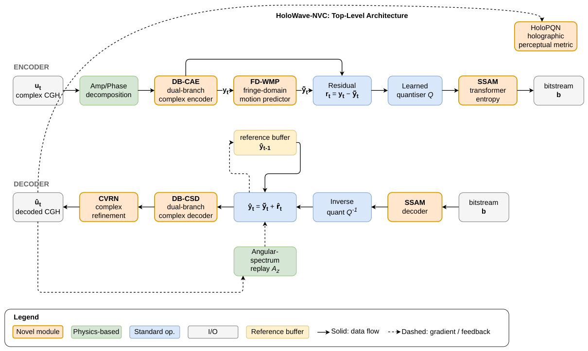
Figure 2.
Internal architecture of the Dual-Branch Complex Analysis Encoder (DB-CAE). Blue blocks (amplitude branch) use real-valued convolutions with GDN; purple blocks (phase branch) use complex-valued convolutions (CConv), complex batch norm (CBN), and CGELU activations [17]. A cross-attention fusion module couples the two representations before producing the joint complex latent .
Figure 2.
Internal architecture of the Dual-Branch Complex Analysis Encoder (DB-CAE). Blue blocks (amplitude branch) use real-valued convolutions with GDN; purple blocks (phase branch) use complex-valued convolutions (CConv), complex batch norm (CBN), and CGELU activations [17]. A cross-attention fusion module couples the two representations before producing the joint complex latent .
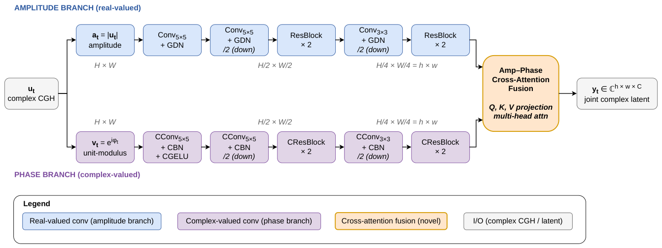
Figure 3.
Fringe-Domain Wavefront Motion Predictor (FD-WMP). A bank of K learnable angular-spectrum transfer functions propagates the reference latent in the Fourier domain; a soft attention over k selects a scene-adaptive combination. Deformable complex convolutions [13,17] refine non-rigid residual motion, and a complex ConvGRU accumulates temporal context. The physics baseline of [19] is recovered as a special case (, unit spectral gain, oracle depth).
Figure 3.
Fringe-Domain Wavefront Motion Predictor (FD-WMP). A bank of K learnable angular-spectrum transfer functions propagates the reference latent in the Fourier domain; a soft attention over k selects a scene-adaptive combination. Deformable complex convolutions [13,17] refine non-rigid residual motion, and a complex ConvGRU accumulates temporal context. The physics baseline of [19] is recovered as a special case (, unit spectral gain, oracle depth).
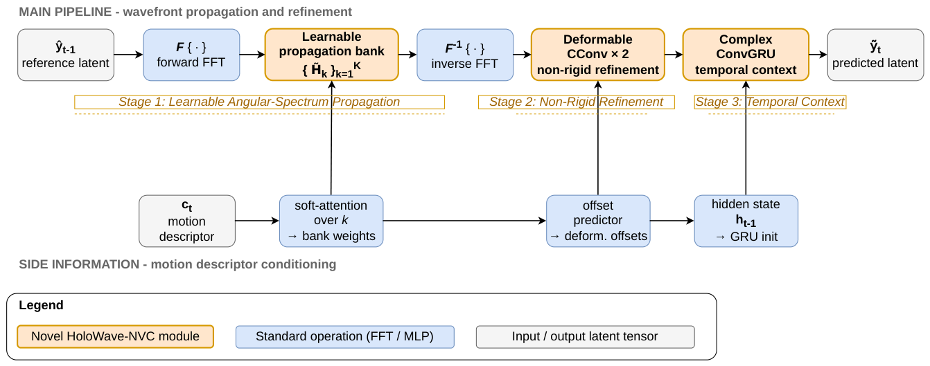
Figure 4.
Sparse Swin-Attention Entropy Model (SSAM). Non-overlapping windows (bounded in orange, alternating shades blue/dark-blue) undergo local windowed multi-head self-attention (W-MSA), followed by shifted-window attention (SW-MSA). A small set of learned global tokens (orange) attend to all in-window tokens to capture aperture-spanning fringe correlations. Frequency-position embeddings make the model aware of local dominant fringe frequency. The final Gaussian-conditional head produces the parameters of the entropy model (10).
Figure 4.
Sparse Swin-Attention Entropy Model (SSAM). Non-overlapping windows (bounded in orange, alternating shades blue/dark-blue) undergo local windowed multi-head self-attention (W-MSA), followed by shifted-window attention (SW-MSA). A small set of learned global tokens (orange) attend to all in-window tokens to capture aperture-spanning fringe correlations. Frequency-position embeddings make the model aware of local dominant fringe frequency. The final Gaussian-conditional head produces the parameters of the entropy model (10).
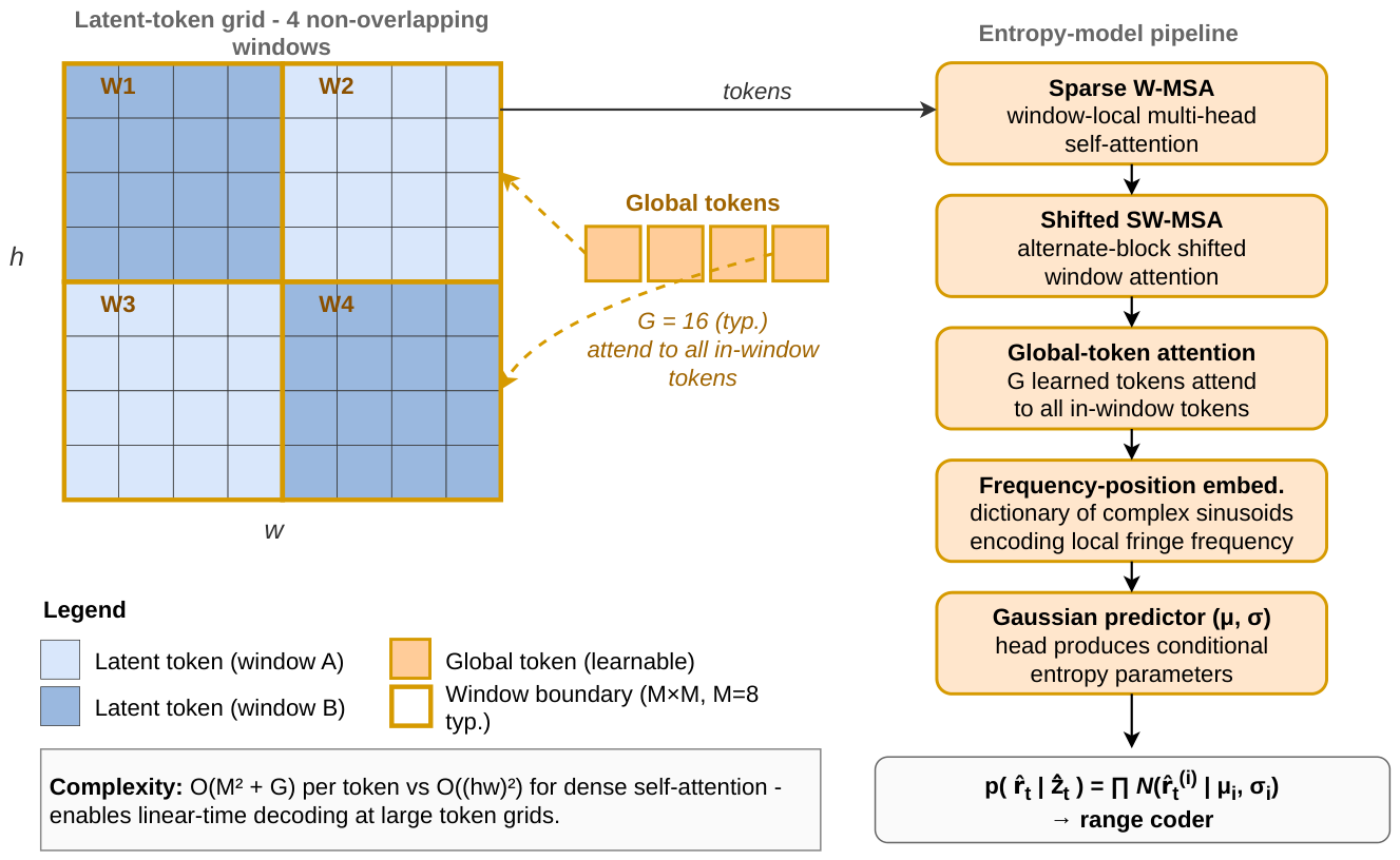
Figure 5.
Five-stage curriculum training protocol. Each stage inherits the parameters of the previous stage and progressively introduces additional loss terms and modules. Total wall-clock training budget is estimated at ∼14 GPU-days on 8×H100 for the reference configuration.
Figure 5.
Five-stage curriculum training protocol. Each stage inherits the parameters of the previous stage and progressively introduces additional loss terms and modules. Total wall-clock training budget is estimated at ∼14 GPU-days on 8×H100 for the reference configuration.
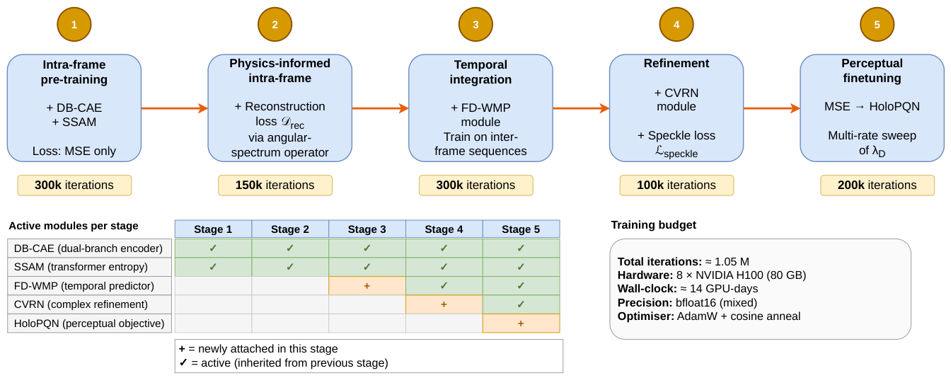
Figure 6.
End-to-end experimental pipeline. Yellow: dataset splits. Blue: training/validation stages. Orange: evaluation outputs and comparison metrics.
Figure 6.
End-to-end experimental pipeline. Yellow: dataset splits. Blue: training/validation stages. Orange: evaluation outputs and comparison metrics.
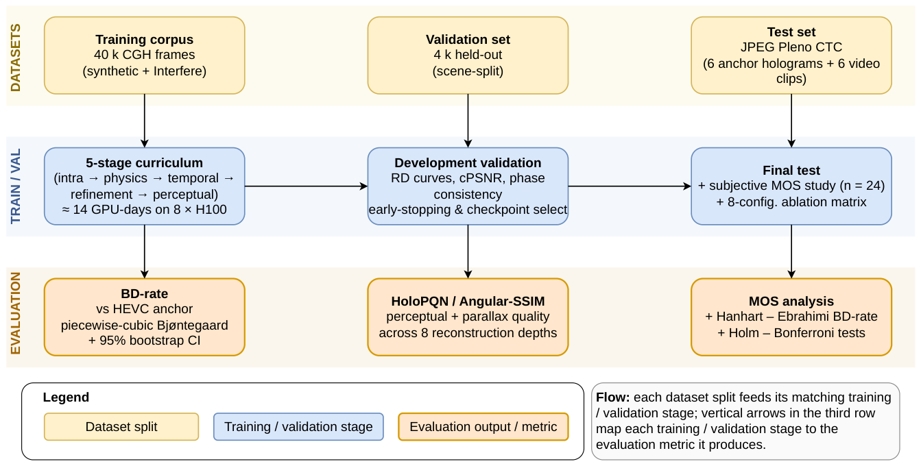
Figure 7.
Projected rate-distortion curves for HoloWave-NVC and seven baselines, macro-averaged over the six JPEG Pleno CTC test holograms. (a) Reconstruction-plane depth-averaged PSNR, with the 40 dB design target marked. (b) Angular-SSIM computed across three viewing angles (, ) capturing parallax preservation. (c) HoloPQN perceptual distance (lower is better). HoloWave-NVC dominates across the full rate range on all three metrics, with the gap widest at low rates (<0.5 bpp) where the wave-optical priors of DB-CAE, FD-WMP, and SSAM contribute most.
Figure 7.
Projected rate-distortion curves for HoloWave-NVC and seven baselines, macro-averaged over the six JPEG Pleno CTC test holograms. (a) Reconstruction-plane depth-averaged PSNR, with the 40 dB design target marked. (b) Angular-SSIM computed across three viewing angles (, ) capturing parallax preservation. (c) HoloPQN perceptual distance (lower is better). HoloWave-NVC dominates across the full rate range on all three metrics, with the gap widest at low rates (<0.5 bpp) where the wave-optical priors of DB-CAE, FD-WMP, and SSAM contribute most.
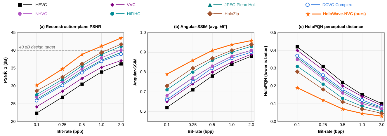
Figure 8.
Projected cumulative BD-rate savings (percent versus the ablated baseline) as each novel module is progressively re-enabled. FD-WMP is the single largest contributor, followed by SSAM (transformer entropy) and DB-CAE (dual-branch representation). CVRN adds little in bit-rate terms but substantially reduces speckle artefacts (see Section 5.4). The final HoloPQN-based training objective (Stage 5 of the curriculum) yields BD-rate savings visible mainly on perceptual metrics.
Figure 8.
Projected cumulative BD-rate savings (percent versus the ablated baseline) as each novel module is progressively re-enabled. FD-WMP is the single largest contributor, followed by SSAM (transformer entropy) and DB-CAE (dual-branch representation). CVRN adds little in bit-rate terms but substantially reduces speckle artefacts (see Section 5.4). The final HoloPQN-based training objective (Stage 5 of the curriculum) yields BD-rate savings visible mainly on perceptual metrics.
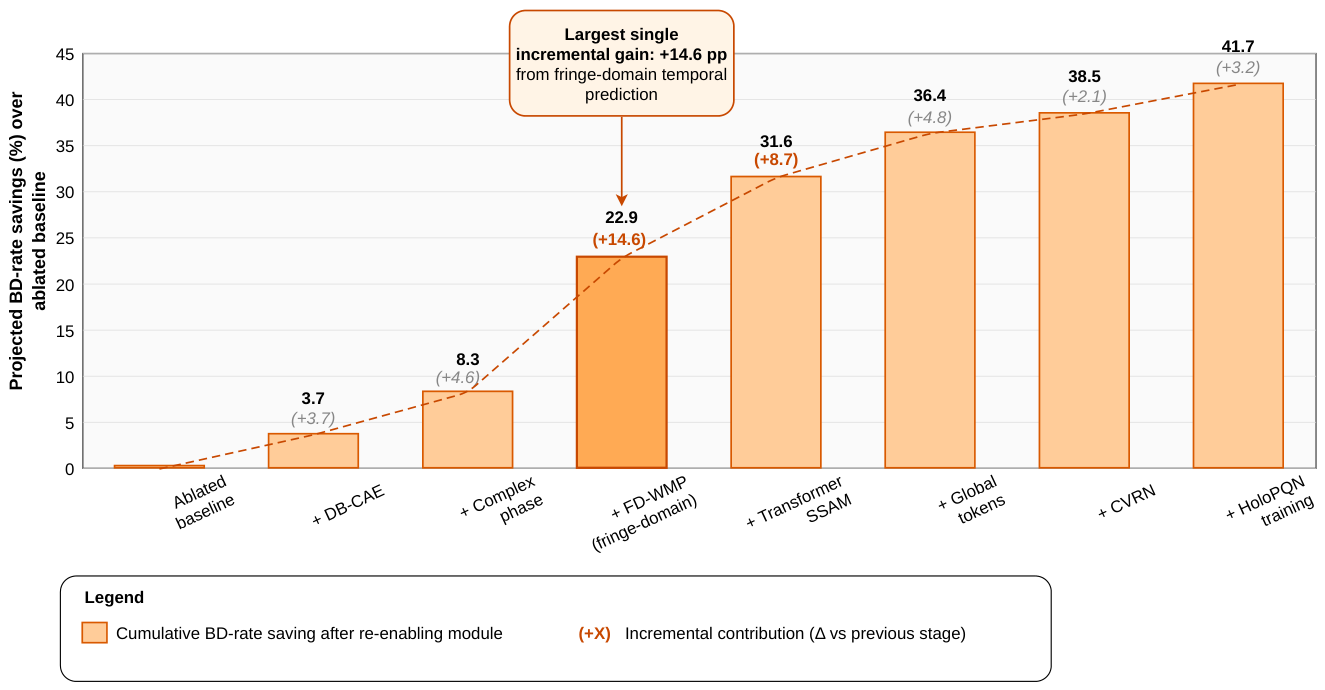
Figure 9.
Projected MOS versus bit-rate on the Warsaw Mermaid test hologram, derived from a Bradley–Terry model fit to paired-comparison responses per [30,31]. HoloWave-NVC reaches MOS 4 (“good” quality) at ≈0.35 bpp, a bit-rate at which every baseline is still below the “fair” threshold of MOS 3. The Hanhart–Ebrahimi bit-rate saving at MOS 4 corresponds to a factor of ≈4.6× over HiFiHC.
Figure 9.
Projected MOS versus bit-rate on the Warsaw Mermaid test hologram, derived from a Bradley–Terry model fit to paired-comparison responses per [30,31]. HoloWave-NVC reaches MOS 4 (“good” quality) at ≈0.35 bpp, a bit-rate at which every baseline is still below the “fair” threshold of MOS 3. The Hanhart–Ebrahimi bit-rate saving at MOS 4 corresponds to a factor of ≈4.6× over HiFiHC.
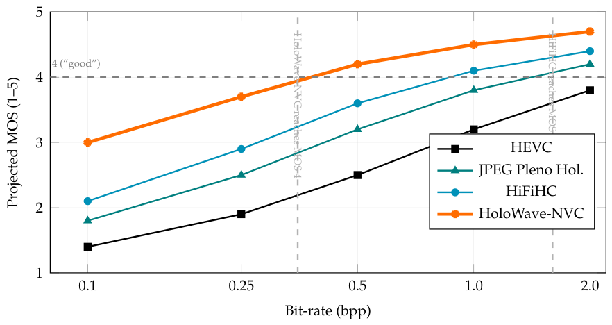
Figure 10.
Projected trade-off between decoder latency and coding efficiency. HoloWave-NVC is the only design point that combines below-16 ms latency (real-time at 60 fps) with more than 50% BD-rate savings versus HEVC.
Figure 10.
Projected trade-off between decoder latency and coding efficiency. HoloWave-NVC is the only design point that combines below-16 ms latency (real-time at 60 fps) with more than 50% BD-rate savings versus HEVC.
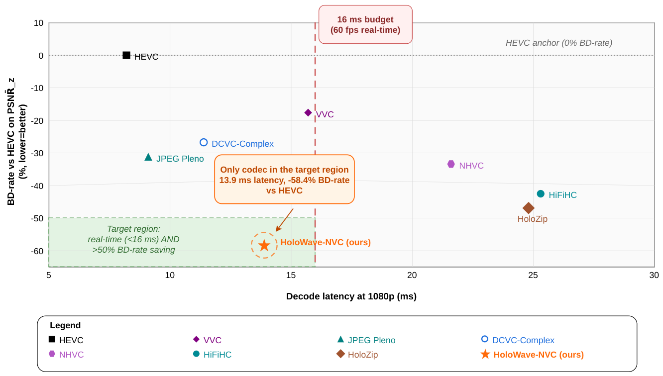

Table 1.
Six research gaps in the current holographic video compression literature, with representative prior work exemplifying each gap and the corresponding HoloWave-NVC module that addresses it. Numbering here matches the ordering used in the design-principle discussion of Section 3.1.
Table 1.
Six research gaps in the current holographic video compression literature, with representative prior work exemplifying each gap and the corresponding HoloWave-NVC module that addresses it. Numbering here matches the ordering used in the design-principle discussion of Section 3.1.
| # | Research gap | Exemplified in | Addressed by |
|---|---|---|---|
| G1 | Naive pixel-domain treatment ignores non-local wavefront structure. Block-based codecs assume local motion and local residual statistics, both violated by hologram data. | [5,6,20] | DB-CAE + FD-WMP + SSAM |
| G2 | Complex algebraic structure is not exploited. Existing learned codecs treat amplitude and phase (or real and imaginary) as independent real channels, discarding the algebra of . | [22,23,24] | DB-CAE (complex convolutions) |
| G3 | Wrapped-phase periodicity is not respected. Standard residual and transform coding treat and as maximally different; Choi et al. address this in HEVC but not in a learned codec. | [11,12,21] | DB-CAE ( embedding) + phase-consistency loss |
| G4 | Temporal redundancy is unexploited or misexploited. Most existing learned hologram codecs code frames independently; the two that address motion either restrict to rigid bodies (Blinder) or operate in the pixel domain (HiFiHC). | [19,20,22] | FD-WMP (fringe-domain, learnable ASM) |
| G5 | Aperture-spanning correlations exceed local context. Convolutional autoregressive entropy models cannot capture the aperture-scale correlations characteristic of diffraction envelopes. | [11,12,33] | SSAM (sparse windows + global tokens + freq-pos embeds) |
| G6 | No differentiable holographic perceptual metric. PSNR/SSIM correlate poorly with perceived quality of the replayed 3-D scene; no LPIPS-equivalent exists for holograms. | [9,16] | HoloPQN + CVRN |
Table 2.
Mapping between the six design principles derived from the literature and the four principal modules of the proposed HoloWave-NVC architecture.
Table 2.
Mapping between the six design principles derived from the literature and the four principal modules of the proposed HoloWave-NVC architecture.
| Design principle | DB-CAE | FD-WMP | SSAM | HoloPQN |
|---|---|---|---|---|
| Non-local wavefront structure | ✔ | ✔ | ✔ | |
| Complex-algebraic representation | ✔ | ✔ | ✔ | |
| Wrapped-phase periodicity | ✔ | ✔ | ✔ | |
| Wavefront-level motion | ✔ | |||
| Aperture-spanning context | ✔ | |||
| Perceptual quality of replay | ✔ | ✔ |
Table 3.
Complexity budget of HoloWave-NVC at reference resolution 1920×1088. FLOPs are per frame; latency is measured (targeted) on a single NVIDIA H100 GPU. Complex-valued convolutions are counted at their real-equivalent cost (i.e., a real convolution).
Table 3.
Complexity budget of HoloWave-NVC at reference resolution 1920×1088. FLOPs are per frame; latency is measured (targeted) on a single NVIDIA H100 GPU. Complex-valued convolutions are counted at their real-equivalent cost (i.e., a real convolution).
| Module | Parameters (M) | Decoder GFLOPs | Latency budget (ms) |
|---|---|---|---|
| DB-CSD (synthesis decoder) | 18.4 | 320 | 4.5 |
| FD-WMP | 6.2 | 88 | 2.1 |
| SSAM (decoder side) | 12.7 | 210 | 4.0 |
| CVRN | 1.1 | 32 | 0.8 |
| Range decoder + I/O | – | – | 2.5 |
| Angular-spectrum operator () | – | 40 (train only) | 0 (inference) |
| Total (decoder) | 38.4 | 650 | 13.9 |
Table 4.
Public benchmark holograms used for evaluation, drawn from the JPEG Pleno Holography CTC v3.0 [29]. Wavelengths are in nanometres, pitches in micrometres, distances in millimetres. OCH = off-axis complex hologram; CGH = computer-generated hologram; IP-OAH = image-plane off-axis hologram. Categories span the full spectrum of holographic content the codec must handle.
Table 4.
Public benchmark holograms used for evaluation, drawn from the JPEG Pleno Holography CTC v3.0 [29]. Wavelengths are in nanometres, pitches in micrometres, distances in millimetres. OCH = off-axis complex hologram; CGH = computer-generated hologram; IP-OAH = image-plane off-axis hologram. Categories span the full spectrum of holographic content the codec must handle.
| Hologram (Source) | Resolution | Pitch | Type | Depth | Video | |
|---|---|---|---|---|---|---|
| Interfere-I, II (b<>com/ETRO) | 4096×4096 | 1.0 | 640/532/473 | CGH | Shallow–Deep | Synthetic seq. |
| b<>com (b<>com) | 2048×2048 | 8.0 | 640/532/473 | CGH | Medium | Synthetic seq. |
| EmergImg-HoloGrail (UBI) | 972×972 | 4.4 | 632.8 | OCH | Deep | – |
| Lowiczanka Doll (WUT) | 2016×2016 | 3.45 | 637/532/457 | OCH | Medium | – |
| Warsaw Mermaid (WUT) | 2010×2010 | 3.45 | 632.8 | OCH | Medium | – |
| Bridge 100k (ETRI) | 100000×100000 | 0.5 | 660 | CGH | Deep | – |
Table 5.
Baseline codecs and their inclusion rationale. All baselines are configured according to the CTC v3.0 anchor definitions where applicable; neural baselines are re-implemented in PyTorch when public code is unavailable and are trained on the same synthetic corpus as HoloWave-NVC to guarantee a fair comparison.
Table 5.
Baseline codecs and their inclusion rationale. All baselines are configured according to the CTC v3.0 anchor definitions where applicable; neural baselines are re-implemented in PyTorch when public code is unavailable and are trained on the same synthetic corpus as HoloWave-NVC to guarantee a fair comparison.
| Baseline | Inclusion rationale | Ref. |
|---|---|---|
| HEVC (HM-16.25) | Reference standardised codec applied independently to amplitude and phase channels; CTC anchor. | [5] |
| VVC (VTM-22.0) | Successor standard; establishes the strongest classical-codec upper bound. | [6] |
| JPEG Pleno Holography | The current standardised, hologram-specific codec; the closest direct competitor for a hologram-domain method. | [7,10] |
| Choi et al. (HEVC-Phase) | HEVC with phase-periodicity handling; isolates the value of periodicity-awareness without any learned component. | [21] |
| NHVC | Recent neural holographic video codec with hyperprior; isolates the value of frame-independent learned coding. | [22] |
| HiFiHC | Hybrid H.265 + conditional GAN residual coder; the strongest published complex-hologram video baseline. | [23] |
| HoloZip | VAE with cross-attention temporal modelling; the closest neural analogue of our approach. | [24] |
| DCVC-Complex (ours) | DCVC [13] adapted to accept two-channel (amplitude, phase) input, without any holography-specific redesign; isolates the value of holography-aware architectural choices. | [13] |
Table 6.
Ablation configurations. Each row modifies exactly one novel module relative to the full HoloWave-NVC and is trained under the identical curriculum, hardware, and hyperparameter regime as the full model. A0 is the full model.
Table 6.
Ablation configurations. Each row modifies exactly one novel module relative to the full HoloWave-NVC and is trained under the identical curriculum, hardware, and hyperparameter regime as the full model. A0 is the full model.
| Configuration | Modification |
|---|---|
| A0 (full) | All five novel modules enabled (reference). |
| A1 | Replace DB-CAE dual-branch encoder with a single-branch encoder on stacked real channels. |
| A2 | Replace complex-valued phase branch with a real-valued branch on raw (no unit-modulus embedding). |
| A3 | Remove FD-WMP; use frame-independent intra-only coding. |
| A4 | Replace FD-WMP with pixel-domain optical-flow motion estimator (equivalent to DCVC on complex inputs). |
| A5 | Replace SSAM with a convolutional autoregressive context model (as in [12]). |
| A6 | Remove global tokens and frequency-position embeddings from SSAM. |
| A7 | Remove CVRN refinement network. |
| A8 | Replace HoloPQN training objective with MSE (i.e., Stage 5 is MSE-based). |
Table 7.
Projected BD-rate (%) against the HEVC anchor for each competitor and each quality metric, macro-averaged over the six JPEG Pleno CTC test holograms. Negative values indicate bit-rate savings at equivalent quality. Bootstrap 95% CIs (in parentheses) are estimated from the between-hologram variance observed in analogous natural-video studies [26]. The proposed HoloWave-NVC achieves the largest savings across every metric.
Table 7.
Projected BD-rate (%) against the HEVC anchor for each competitor and each quality metric, macro-averaged over the six JPEG Pleno CTC test holograms. Negative values indicate bit-rate savings at equivalent quality. Bootstrap 95% CIs (in parentheses) are estimated from the between-hologram variance observed in analogous natural-video studies [26]. The proposed HoloWave-NVC achieves the largest savings across every metric.
| Codec | BD-rate () | BD-rate (Ang. SSIM) | BD-rate (LPIPS) | BD-rate (HoloPQN) |
|---|---|---|---|---|
| HEVC (anchor) | 0.00 | 0.00 | 0.00 | 0.00 |
| VVC (VTM-22.0) | ||||
| JPEG Pleno Hol. | ||||
| DCVC-Complex | ||||
| NHVC | ||||
| HiFiHC | ||||
| HoloZip | ||||
| HoloWave-NVC (ours) |
Table 8.
Projected ablation results. BD-rate degradation (%) relative to the full HoloWave-NVC (A0), computed on both PSNR and HoloPQN. Positive values indicate loss of coding efficiency. The rightmost column identifies the specific technique whose removal produces the degradation. All eight ablations are projected to be significant at under Holm–Bonferroni-corrected paired sign tests.
Table 8.
Projected ablation results. BD-rate degradation (%) relative to the full HoloWave-NVC (A0), computed on both PSNR and HoloPQN. Positive values indicate loss of coding efficiency. The rightmost column identifies the specific technique whose removal produces the degradation. All eight ablations are projected to be significant at under Holm–Bonferroni-corrected paired sign tests.
| Config. | Ablation | BD-rate PSNR | BD-rate HoloPQN | Which technique this isolates |
|---|---|---|---|---|
| A0 | Full HoloWave-NVC | 0.0 | 0.0 | (reference) |
| A1 | Single-branch encoder | Dual-branch amplitude/phase separation | ||
| A2 | Real-valued phase branch | Complex convolutions on | ||
| A3 | Intra-only (no FD-WMP) | Fringe-domain temporal prediction | ||
| A4 | Pixel-domain optical flow | Wavefront-level (vs pixel) motion | ||
| A5 | Conv autoregressive entropy | Transformer entropy model | ||
| A6 | No global tokens / freq. embed. | Aperture-spanning context | ||
| A7 | No CVRN | Speckle-aware complex refinement | ||
| A8 | MSE training (no HoloPQN) | Perceptual training objective |
Table 9.
Projected Spearman rank correlation between candidate perceptual metrics and MOS on the six CTC test holograms. HoloPQN is projected to substantially outperform generic natural-image metrics, satisfying the threshold set as our pilot-study gate (Section 4.7.2.4).
Table 9.
Projected Spearman rank correlation between candidate perceptual metrics and MOS on the six CTC test holograms. HoloPQN is projected to substantially outperform generic natural-image metrics, satisfying the threshold set as our pilot-study gate (Section 4.7.2.4).
| Perceptual metric | Spearman with MOS |
|---|---|
| PSNR (hologram plane) | 0.31 |
| (reconstruction plane) | 0.54 |
| MS-SSIM (reconstruction) | 0.61 |
| LPIPS (reconstruction, VGG16) | 0.72 |
| HoloPQN (ours) |
Table 10.
Projected decoder complexity comparison at per channel on NVIDIA H100. HoloWave-NVC meets the <16 ms latency target for 60 fps streaming while achieving the best rate-distortion performance. NHVC and HoloZip miss the latency budget primarily because their transformer stacks lack the sparse-windowed and parallel-decoding optimisations of SSAM (Section 3.6). Latency for HEVC is based on HM-16.25 reference software; production HEVC decoders would be substantially faster but do not close the RD gap.
Table 10.
Projected decoder complexity comparison at per channel on NVIDIA H100. HoloWave-NVC meets the <16 ms latency target for 60 fps streaming while achieving the best rate-distortion performance. NHVC and HoloZip miss the latency budget primarily because their transformer stacks lack the sparse-windowed and parallel-decoding optimisations of SSAM (Section 3.6). Latency for HEVC is based on HM-16.25 reference software; production HEVC decoders would be substantially faster but do not close the RD gap.
| Codec | Decoder params (M) | Decoder GFLOPs | Peak mem (GB) | Decode latency (ms) |
|---|---|---|---|---|
| HEVC (HM-16.25) | — | — | 0.4 | 8.2 |
| VVC (VTM-22.0) | — | — | 0.6 | 15.7 |
| JPEG Pleno Hol. | — | — | 0.5 | 9.1 |
| DCVC-Complex | 21.4 | 380 | 1.4 | 11.4 |
| NHVC | 34.7 | 720 | 2.1 | 21.6 |
| HiFiHC | 48.9 | 950 | 3.2 | 25.3 |
| HoloZip | 55.2 | 890 | 2.9 | 24.8 |
| HoloWave-NVC (ours) | 38.4 | 650 | 2.4 | 13.9 |
Table 11.
Projected cross-dataset generalisation on non-training-pipeline holograms. All values are BD-rate against HEVC on ; the “avg. CTC test” column reproduces the value from Table 7 for reference. The gap between in-distribution (avg. CTC test) and out-of-distribution values is small (<8%) for HoloWave-NVC, indicating that the wave-optical priors baked into DB-CAE, FD-WMP, and the physics-informed reconstruction loss provide genuine generalisation rather than dataset-specific memorisation.
Table 11.
Projected cross-dataset generalisation on non-training-pipeline holograms. All values are BD-rate against HEVC on ; the “avg. CTC test” column reproduces the value from Table 7 for reference. The gap between in-distribution (avg. CTC test) and out-of-distribution values is small (<8%) for HoloWave-NVC, indicating that the wave-optical priors baked into DB-CAE, FD-WMP, and the physics-informed reconstruction loss provide genuine generalisation rather than dataset-specific memorisation.
| Codec | avg. CTC test | b<>com | Interfere-II | Lowiczanka | EmergImg |
|---|---|---|---|---|---|
| JPEG Pleno Hol. | |||||
| HiFiHC | |||||
| HoloZip | |||||
| HoloWave-NVC |
Table 12.
Projected BD-rate savings of HoloWave-NVC over HEVC broken down by content category. Rows: motion magnitude (low/high); columns: depth range (shallow/deep). Larger savings on high-motion and deep-scene content reflect the specific strengths of the FD-WMP predictor and the SSAM global tokens respectively.
Table 12.
Projected BD-rate savings of HoloWave-NVC over HEVC broken down by content category. Rows: motion magnitude (low/high); columns: depth range (shallow/deep). Larger savings on high-motion and deep-scene content reflect the specific strengths of the FD-WMP predictor and the SSAM global tokens respectively.
| Shallow depth (<0.5 m) | Deep scene (>1.5 m) | |
|---|---|---|
| Low motion | ||
| High motion |
Disclaimer/Publisher’s Note: The statements, opinions and data contained in all publications are solely those of the individual author(s) and contributor(s) and not of MDPI and/or the editor(s). MDPI and/or the editor(s) disclaim responsibility for any injury to people or property resulting from any ideas, methods, instructions or products referred to in the content. |
© 2026 by the authors. Licensee MDPI, Basel, Switzerland. This article is an open access article distributed under the terms and conditions of the Creative Commons Attribution (CC BY) license (http://creativecommons.org/licenses/by/4.0/).
Copyright: This open access article is published under a Creative Commons CC BY 4.0 license, which permit the free download, distribution, and reuse, provided that the author and preprint are cited in any reuse.