

Submitted:
18 August 2026
Posted:
19 August 2026
You are already at the latest version
Abstract
World Action Models (WAMs) improve planning by incorporating future world evolution into action generation, yet existing methods allocate a fixed imagination budget to every scene. We propose RISE (Refining Imagination through SElective Rollout), a system-level adaptive imagination framework that makes sequential ROLL/STOP decisions according to the expected planning benefit of continued rollout. At each step, a Latent Evaluator estimates the risk revealed by the current prefix and how much planning could improve if imagination continues, while a Rollout Gate weighs this expected benefit against additional computation cost. Since factual driving logs expose only one realized future, we further construct CounterDrive, a counterfactual dataset with diverse outcomes and risk levels, to enrich future dynamics and provide localized risk supervision. Each retained sample undergoes expert verification and annotation of trajectory validity, incident onset, and causal category, providing a reusable resource for safety-critical world-modeling research. Experiments on NAVSIM and nuScenes show that RISE achieves the best overall planning performance while reducing unnecessary rollout, with additional transfer results supporting its plug-in generality across WAM architectures.
Keywords:
world action model
; autonomous driving
1. Introduction
End-to-end autonomous driving [1,2] is moving beyond direct trajectory regression toward models that reason about the future before acting [3,4]. World Action Models (WAMs) [5,6] incorporate predicted world evolution into planning, allowing policies to evaluate actions through their consequences rather than the current observation alone. This capability is particularly relevant to driving, where similar visual contexts can lead to different outcomes as the ego vehicle and surrounding agents interact. Consequently, recent methods [7,8] employ latent future prediction, action-conditioned dynamics, or world-model-based policy learning to improve planning under interaction and uncertainty.
However, future imagination adds inference cost because latent futures must be generated before an action can be produced. As illustrated in Figure 1(a)–(c), existing WAMs [9,10,11,12] organize this computation differently. Shared-backbone models perform prediction and planning from a common representation through an imagine-and-plan design. Cascaded models complete a future rollout before passing it to the Planner through an imagine-then-plan design. Other approaches remove test-time imagination and plan directly from the observation. Despite these differences, their inference schedules are specified globally. They do not reassess after each partial rollout whether the current prefix is sufficient for planning or continued prediction is likely to improve the final decision.
We refer to this missing decision signal as Future Planning Gain. At rollout step, its profile measures the change in planning score associated with each valid continuation relative to stopping with the current prefix. By expressing continuation utility in planning score, it directly connects additional rollout to downstream planning quality. Because each predicted latent updates the current prefix and the available future evidence, the gain may change throughout rollout. Therefore, it should be re-estimated after each step and used as a sequential stopping signal rather than to select a final rollout depth in advance.
This perspective captures the varying utility of imagination without dividing scenes into predefined easy and difficult categories. The observation or an early prefix may already support a stable trajectory, so continuing offers little gain and only increases latency. Alternatively, the current prefix may leave an interaction unresolved, and an additional predicted step may change the preferred plan. In either case, the decision is local: the model should Roll when the expected improvement justifies its cost and Stop otherwise. Repeating this decision produces a horizon ranging from zero rollout to the dataset-specific maximum.
Building on this principle, we introduce RISE (Refining Imagination through SElective Rollout), the plug-in adaptive imagination framework illustrated in Figure 1(d). RISE augments an Encoder–Predictor–Planner WAM with a lightweight Scheduler composed of a Latent Evaluator and a Rollout Gate. At each step, the Evaluator predicts a Risk Profile summarizing the planning-relevant risk already revealed and a Future Planning Gain Profile describing the improvement available through continued rollout. The Gate weighs the predicted gain against computation cost and makes the current binary decision. Under Roll, the Predictor appends one future latent and the Scheduler evaluates the updated prefix again. Under Stop, the selected prefix is passed once to the Planner. The Gate does not predict the final horizon directly. Therefore, the effective horizon emerges from repeated Roll/Stop decisions.
The two Evaluator signals require different supervision. Planning scores obtained by stopping at every valid prefix provide direct Future Planning Gain targets: the score difference between a continued and current prefix measures the realized benefit of continuation. Risk learning faces a different limitation because factual logs record only the future that occurred and leave plausible safety-critical alternatives unseen. We construct CounterDrive to augment selected contexts with diverse counterfactual outcomes and risk levels. Accepted clips enrich future-latent prediction, while verified factual–counterfactual incident pairs provide temporally localized Risk Profile supervision. Consequently, all-horizon planning outcomes teach how planning changes under continuation, while CounterDrive improves sensitivity to risks revealed along that process.
Extensive experiments on NAVSIM and nuScenes validate the effectiveness of RISE. It achieves 91.5 PDMS and 90.8 EPDMS on NAVSIM v1 and v2, respectively, while obtaining state-of-the-art trajectory accuracy and collision performance on nuScenes. Further analyses show that CounterDrive improves hazard discrimination and that the Scheduler transfers to another architecture without modifying its Predictor or Planner, supporting both adaptive imagination and architectural generality. Our contributions are summarized as follows:
- We propose RISE, a plug-in adaptive imagination framework for WAMs that uses Future Planning Gain to make sequential Roll/Stop decisions, yielding a scene-dependent rollout horizon while balancing planning quality and inference cost.
- We construct CounterDrive, a counterfactual driving dataset with diverse interaction outcomes and risk levels, supporting both RISE training and safety-critical world modeling research.
- Experiments on driving benchmarks show that RISE achieves state-of-the-art planning performance with lower rollout cost, while its transfer to other WAM architecture supports plug-in generality.
2. Related Works
2.1. World Action Models
World action models (WAMs) extend predictive world modeling [13,14] with executable action generation. Rather than directly mapping observations to actions, they use future prediction to learn physical dynamics and state–action correspondences. Unified Video Action Model [15] learns a shared video–action latent space for forward prediction, inverse dynamics, and real-time control. Cosmos Policy [16] adapts pretrained video diffusion models to jointly predict future states, actions, and values. LingBot-VA [17], DreamZero [18], MotuBrain [19], and WLA-0 [20] further scale WAMs toward language-conditioned, long-horizon, and cross-embodiment control. However, most existing WAMs treat test-time imagination as a fixed architectural choice.
2.2. Autonomous Driving World Models
Driving world models predict scene evolution from historical observations and ego actions [21]. ReSim [22] further studies reliable simulation for autonomous driving. GAIA-1 [23] and DriveDreamer [24] generate controllable futures from video, text, and action conditions. OccWorld [25] models future 3D occupancy, while HERMES [26] and UniFuture [27] couple generation with scene understanding or geometric perception. DriveDreamer4D [28] uses generated futures to improve 4D scene representations. More recent methods emphasize planning-oriented latent dynamics: Epona [29] integrates autoregressive diffusion with trajectory planning, whereas Latent-WAM [9], DriveFuture [30], and DreamerAD [10] learn compact future states for end-to-end planning or reinforcement learning. Despite their different representations, these methods generally use a fixed imagination strategy, whereas RISE allocates future reasoning according to scene-dependent planning utility.
3. CounterDrive
Factual driving logs contain only realized futures and provide limited safety-critical alternatives. Therefore, we construct CounterDrive from selected NAVSIM and nuScenes scenes. Each retained counterfactual clip is associated with its factual source, forming pairs within the selected subset rather than covering the complete datasets.
3.1. Counterfactual Video Generation
For each selected source key frame, the prompt combines a fixed instruction, a scene description, and an incident description specifying the event location and involved object. Prompts additionally constrain the camera viewpoint, road geometry, background, and initial traffic configuration so that the generated clip remains anchored to the source scene. Conditioned on the key frame and prompt, Wan 2.7 generates a 10-second video at 1080p resolution, which is sampled at 2 Hz into 20 frames.
3.2. Trajectory Annotation
We apply OpenVO [31] to recover the frame-wise ego poses:
The corresponding ego-motion actions are computed from adjacent poses:
3.3. Human Verification and Annotation
Annotators verify ego-motion consistency, identify the first incident frame, mark generation distortions, and categorize each clip as normal, caused by non-ego behavior, or caused by ego behavior. A recovered trajectory is marked invalid when it disagrees with the visually observed ego motion. For ego-caused incidents, annotators also record recommended avoidance or stopping actions as clip-level metadata. Clips with severe distortion or unreliable motion are removed. Accepted clips supervise future prediction, while verified incident pairs provide temporally localized risk-ranking supervision.
After filtering, CounterDrive contains 2,432/511 training/test clips from nuScenes and 5,013/1,000 from NAVSIM. Unpaired factual samples remain available for standard training objectives. Additional construction and annotation details are provided in the Appendix.
4. RISE
We propose RISE (Refining Imagination through SElective Rollout), a plug-in adaptive imagination framework for World Action Models. As shown in Figure 2, RISE augments an Encoder–Predictor–Planner WAM with a lightweight Scheduler composed of a Latent Evaluator and a Rollout Gate. The Evaluator estimates the planning risk revealed by the current future prefix and the potential gain of deeper rollout, while the Gate determines whether additional imagination is worth its computation cost.
4.1. Problem Formulation
Let c denote the current driving context, the future trajectory over planning horizon P, and the future world representation over a maximum rollout horizon H. A standard World Action Model uses a fixed rollout depth for every scene:
RISE instead makes the effective rollout depth scene-dependent. Given an imagined prefix , where , the Scheduler determines whether the current prefix is sufficient for planning:
where controls the preference for computation cost.
Our RISE models
Here, is selected independently for each scene. When , the model plans directly from the observed context; when , it recovers the full-rollout behavior of a standard WAM.
4.2. World Action Model Architecture
4.2.1. Encoder
We use a frozen V-JEPA 2 [32] image encoder with a ViT-L backbone to encode front-camera observations into latent tokens. Four input frames are resized to and processed using patches and non-overlapping two-frame tubelets. The Encoder produces two observed latent time steps, each containing 512 spatial tokens of dimension 1024.
4.2.2. Predictor
We adopt a frame-causal ego motion conditioned Transformer with 12 layers, a hidden dimension of 384, and 12 attention heads. Starting from the observed latent tokens, the Predictor autoregressively generates up to future latent steps, each corresponding to two raw video frames. Hereafter, denotes the dataset-specific realization of the maximum horizon H. Ego-motion conditions are represented by relative pose changes computed between adjacent ego poses. The Predictor uses no route command, additional state input, or camera extrinsic.
4.2.3. Planner
We employ a 12-layer diffusion Transformer with a hidden dimension of 384 and 12 attention heads. The Planner conditions on the observed tokens and the selected future prefix, distinguished by learned source embeddings, together with the observed ego-motion history and current ego kinematics. It generates six candidate trajectories using a variance-preserving diffusion process with 20 DPM-Solver++ [33] sampling steps. Each candidate contains eight future poses at s intervals, represented as . Candidate selection and dataset-specific scoring details are provided in the Appendix.
4.3. Adaptive Rollout Scheduler
At rollout depth h, the Scheduler decides whether to stop with the currently available future prefix or generate one additional latent step. It is guided by the predicted Future Planning Gain of continuing rollout and computation cost.
4.3.1. Latent Evaluator
Given the observed latent and imagined prefix , the Latent Evaluator predicts a Risk Profile and a Future Planning Gain Profile:
where estimates the trajectory risk associated with the prefix ending at depth k, while predicts the Future Planning Gain of continuing from depth h to j, measured relative to stopping with the current prefix. Thus, summarizes the risk already exposed, whereas summarizes the potential planning gains available from continued rollout.
4.3.2. Rollout Gate
For , we construct
where denotes token pooling, is a learned empty-prefix embedding, and are zero-padded to length , is the cumulative cost, and . Given computation preference , the Gate predicts
The sign of indicates whether the predicted planning gain available from continued rollout justifies its additional cost. The Scheduler applies
For Roll, the Predictor appends one future latent step and the Scheduler evaluates the extended prefix. For Stop, the selected prefix is risk-refined when and passed once to the Planner. Refinement is skipped when , and rollout terminates at by construction.
4.4. Three-Stage Training
RISE is trained in three stages. Stage I trains the Predictor and an initial variable-prefix Planner. Stage II learns planning-oriented risk and Future Planning Gain. Stage III converts these signals into a cost-aware stopping policy.
4.4.1. Stage I: Predictor and Initial Planner
The Predictor recursively generates the maximum dataset-specific prefix . It is trained on real and accepted CounterDrive sequences using teacher-encoded future latents:
where is the target latent, denotes the stop-gradient. For CounterDrive sequences, the ego-motion conditions are computed from adjacent recovered poses. We then train an initial Planner using real trajectory supervision:
The Encoder, Predictor, and are frozen when constructing the subsequent training targets.
4.4.2. Stage II: Latent Evaluator and Guided Planner
For each real prefix, produces candidate trajectories whose planning risk is computed by a fixed geometry-based evaluator:
The evaluator includes the common candidate-selection rule and geometry-based risk terms, whose definitions are provided in the Appendix.
CounterDrive contributes paired supervision only when a verified factual–counterfactual pair is available. Let denote the verified pairs in which the counterfactual future contains an annotated incident and is ranked as riskier than its factual source. For a pair i, the annotated incident frame is mapped to latent step , and we define
Real samples without a paired counterfactual clip are excluded only from this ranking term. The complete Risk Profile objective is
where uses the annotated incident onset for temporally localized risk calibration. Its detailed construction and loss weights are provided in the Appendix.
After learning the Risk Profile, we refine each non-empty prefix using a small norm-constrained update:
For , we define and skip refinement. The final Planner is trained at all valid rollout depths:
We evaluate at every rollout depth and denote its dataset-specific planning score by
The Future Planning Gain target is
The loss details are in the Appendix.
4.4.3. Stage III: Rollout Gate
Finally, we freeze other modules and train the Rollout Gate as a cost-aware stopping policy. For each real sample, we enumerate all valid rollout depths and record and cumulative cost . For a computation preference , the best remaining cost-adjusted gain is
The continuation target and Gate objective are
At the maximum depth, rollout stops by construction. Full-horizon enumeration is used only to construct training targets.
5. Experiments
5.1. Implementation Details
All experiments are implemented in PyTorch using bfloat16 precision. The training is conducted on 8 × NVIDIA A100 GPUs with a per-GPU batch size of 4. Videos are sampled at 2 Hz and resized to . Each clip contains four observed frames and a dataset-specific future horizon. With two-frame tubelets, we set and . We train for 20 epochs with a learning rate of and for 50 epochs with using AdamW. The scheduler is trained for 50 epochs with a learning rate of . Latent guidance performs two gradient steps with a step size of and a maximum update norm of . We use normalized rollout costs and evaluate , with as the default.
5.2. Main Results
We compare RISE with representative driving WAMs in the perception-free setting, including DrivingGPT [36], LAW [37], World4Drive [38], Epona [29], DriveVLA-W0 [39], PWM [40], DreamerAD [10], DriveLaW [34], Drive-JEPA [7], DAWN [12], EponaV2 [35], DriveFuture [30], and Latent-WAM [9]. As shown in Table 1, Table 2 and Table 3, RISE achieves the best overall planning performance on both NAVSIM V1 and V2, reaching 91.5 PDMS and 90.8 EPDMS, respectively. It surpasses the strongest baselines by 0.8 points on V1 and 0.9 points on V2. On NAVSIM V1, RISE improves the previous best EP and TTC by 2.9 and 1.9 points, respectively. On NAVSIM V2, it ranks first or ties for first on seven of the nine component metrics, demonstrating strong performance across safety, compliance, and planning quality. RISE also establishes state-of-the-art results on nuScenes, achieving the lowest average L2 error of 0.31 m and collision rate of 0.10. These results demonstrate that adaptive rollout improves planning across evaluation settings.
5.3. Ablation Studies
5.3.1. Ablation on Key Components
Table 4 isolates the Scheduler and CounterDrive under the same backbone and training settings. CounterDrive alone raises EPDMS/PDMS from 88.9/89.7 to 89.8/90.5, indicating that counterfactual futures provide useful supervision for future representation learning. The Scheduler alone reaches 90.4/91.2, confirming that scene-dependent rollout allocation independently improves planning. Combining both yields the best results of 90.8/91.5, showing their complementary roles: CounterDrive enriches future supervision, while the Scheduler allocates additional imagination where it remains useful.
5.3.2. Ablation on Adaptive Rollout Method
Table 5 compares the Scheduler with Random Stop and Latent Margin. Random Stop assigns each sample a reproducible horizon from , whereas Latent Margin stops when consecutive latents converge. Random Stop provides the lowest latency of 264.075 ms but reaches only 89.5 EPDMS. Latent Margin averages 2.98 rollouts and incurs 308.532 ms latency, yet obtains only 89.7 EPDMS. In contrast, the Scheduler achieves 90.8 EPDMS with 2.40 rollouts and 287.429 ms latency. It shows that effective stopping should reflect the planning gain rather than random allocation or latent convergence alone.
5.4. Further Analysis
5.4.1. Is Adaptive Rollout Necessary?
To examine whether a single rollout depth can serve all scenes, we evaluate every sample at fixed depths and group it by the depth yielding its highest planning score. Figure 3 shows substantial groups at every depth: 1,248 scenes perform best without rollout, whereas 4,036 and 2,180 scenes favor depths 3 and 4, respectively. For the group, increasing the depth from 0 to 4 reduces EPDMS from 89.9 to 88.4. Conversely, for the group, it improves from 88.5 to 91.1. Thus, deeper imagination benefits some scenes but is unnecessary or even detrimental to others. The examples in Figure 4 provide an intuitive view of this variation. The examples present open roads and limited immediate interaction, for which the observation already provides sufficient evidence for planning. The examples contain traffic lights, vehicles, or road construction, introducing interactions that benefit from modest future context. The cases involve dense pedestrian flow or crossing vehicles, where future evolution is ambiguous and additional prediction is valuable. These examples explain why the best-performing depth varies across scenes and why no fixed rollout budget is uniformly optimal.
5.4.2. Does CounterDrive Improve Safety-Critical Evaluation?
To assess whether CounterDrive improves safety-critical evaluation, we evaluate identical models with and without CounterDrive on the held-out counterfactual test set. As shown in Table 6, the model without CounterDrive remains close to random risk ranking, with AUC scores of 0.49–0.52 and an accident-recognition accuracy of 0.51. CounterDrive increases the four horizon-specific AUC scores to 0.93–0.96 and accuracy to 0.96, demonstrating substantially improved risk discrimination and accident awareness.
5.4.3. Can RISE Benefit Other Paradigm?
To evaluate whether the proposed Scheduler generalizes beyond our base WAM, we reproduce DAWN, a representative World–Action Interactive Model, and integrate the Scheduler without modifying its Predictor or Planner. As shown in Table 7, the resulting model improves PDMS from 89.1 to 90.3. Consistent gains are also observed in NC, DAC, EP, and TTC, with particularly clear improvements of 2.7 points in EP and 2.3 points in TTC, while retaining a perfect collision score. These results suggest that the Scheduler can serve as a plug-in adaptive computation module for different world–action modeling paradigms, rather than being tied to a specific WAM.
5.4.4. Can RISE Generate Plausible and Safe Trajectories?
Figure 5 compares RISE with Drive-JEPA across representative scenes. In the intersection and turning cases of Figure 5(b)–(d), Drive-JEPA exhibits lateral or directional deviations from the local lane geometry, whereas RISE remains within feasible lane corridors and closely matches the human trajectory. In the curved-road cases of Figure 5(a) and (e), RISE likewise follows the reference closely, including at , while Drive-JEPA shows greater lateral deviation. These examples show that RISE produces plausible, lane-consistent trajectories across varied road structures and selected rollout depths.
6. Conclusion
We presented RISE, a plug-in adaptive imagination framework that replaces fixed-depth WAM rollout with scene-dependent computation. Its Latent Evaluator estimates current risk and Future Planning Gain, allowing the Scheduler to make cost-aware sequential Roll/Stop decisions. We also introduced CounterDrive for counterfactual future learning and risk evaluation. Experiments on nuScenes and NAVSIM demonstrate competitive planning performance while balancing planning quality and inference cost.
7. Limitations
Although adaptive rollout is designed as a general principle for world action models, our experiments currently focus on autonomous driving, and its applicability to other domains remains to be explored. Furthermore, due to the cost of generating and filtering counterfactual samples, CounterDrive does not yet provide one-to-one coverage of the NAVSIM training set. Nevertheless, the primary goal of this work is to establish the necessity of scene-adaptive rollout, which is consistently supported by our experiments. Future work will extend the evaluation to broader domains and further scale the counterfactual dataset.
Acknowledgments
This work was supported in part by the Research and Application of Key Technologies for L4 End-to-End Autonomous Driving Based on Multi-modal Large Language Models under Grant 202423dl2050005, and in part by Research and Application of the Next-Generation General-Purpose Intelligent Robot Brain (Robo-GPT) under Grant 2024zd01.
Appendix A. Implementation Details
Compute and data.
We implement RISE in PyTorch. The WAM and diffusion planners are trained with bfloat16 precision on eight NVIDIA A100 GPUs using a per-GPU batch size of 4, giving an effective batch size of 32. The lightweight Evaluator and Rollout Gate are trained offline in FP32 on one A100. We use four data-loading workers per process with pinned and persistent workers. Front-camera videos are sampled at 2 Hz and resized to . Each clip contains four observed frames. With a spatial patch size of 16 and a temporal tubelet size of 2, the four observations correspond to two observed latent steps. We set the maximum rollout horizons to and . Horizontal flipping, motion shifting, GridMask, AutoAugment, and random erasing are disabled.
World Action Model.
The visual encoder is a Drive-JEPA ViT-L/16 with causal attention. The action-conditioned Predictor contains 12 Transformer blocks with a hidden dimension of 384, 12 attention heads, rotary positional embeddings, and activation checkpointing. Each rollout step is conditioned on a three-dimensional ego-action vector. Ego-state conditioning, route-command conditioning, camera extrinsics, and parallel future prediction are disabled. A frozen Token-AE represents each latent frame using 128 tokens arranged on an latent grid. It uses a four-layer encoder, a two-layer decoder, and a two-layer causal temporal module with 16 attention heads and zero dropout. During Planner, Evaluator, and Scheduler training, the visual encoder and Predictor remain frozen.
Dynamic planners.
Both and use the same diffusion Transformer architecture with 12 layers, a hidden dimension of 384, 12 attention heads, an MLP ratio of 4, and zero dropout. The variance-preserving diffusion process uses and . At inference, the Planner performs 20 denoising steps and generates trajectory modes. Each pose is represented by with a temporal interval of . The classification, regression, velocity, and yaw losses are weighted by , , , and , respectively. The confidence temperature is 1.5, with classification and ignore thresholds of 2.0 and 0.2. The adaptive winner-take-all temperature starts at 8.0, decays with a factor of 0.984, and is lower-bounded by 0.1. During dynamic-prefix training, the full prefix is sampled with probability 0.25, while the remaining probability is distributed uniformly over .
Planner optimization.
We optimize both planners using AdamW with , , and a weight decay of 0.04. For , training lasts 20 epochs; the learning rate is linearly warmed up from to during the first two epochs and then cosine-decayed to zero. For , training lasts 50 epochs; the learning rate is warmed up from to during the first five epochs and then cosine-decayed to zero. We use deterministic execution and fixed diffusion noise for validation.
Evaluator and latent guidance.
The Evaluator first mean-pools the spatial tokens of each latent frame, applies LayerNorm, and encodes the prefix using a one-layer causal GRU with a hidden dimension of 512 and zero dropout. Two linear heads produce its task-evaluation profiles. The initial warm-up is performed for one epoch with 256 updates, a batch size of 4, and a learning rate of . Real samples use a Huber loss with , while counterfactual hazard and trajectory-quality ranking losses use unit weights and a margin of 1.0. Local calibration uses one epoch with 256 updates, a batch size of 1, and a learning rate of . For each latent prefix, we sample four Gaussian perturbations with a scale of 0.05 and clip their per-token norm to 0.25; the local ordering loss has weight 1.0 and margin 0.1. The second profile head is subsequently calibrated for one epoch with a batch size of 1 and a learning rate of , while the shared prefix encoder is frozen. All Evaluator stages use AdamW with the same , , and weight decay as the planners.
Rollout Gate.
The Rollout Gate applies LayerNorm followed by two 128-dimensional fully connected layers with GELU activations. It is distilled from complete horizon-wise utility curves for 50 epochs using AdamW, a batch size of 1, a constant learning rate of , and a weight decay of 0.04. Its classification loss uses a temperature of 0.05, and the Smooth-L1 utility-regression term is weighted by 0.5. We define normalized rollout costs as and train the conditional Gate with , using by default. Latent guidance performs two gradient steps on the latest imagined prefix with a step size of 0.05 and a maximum update norm of 0.25. The guided latent is detached before being passed to the Planner. Unless otherwise specified, all experiments use random seed 239.
Appendix B. More Training Details of RISE
Notation and conventions.
We use H for the abstract maximum latent rollout horizon and for its dataset-specific realization. In our experiments, and . We use P for the number of future poses in a planned trajectory and J for the number of Planner modes. The indices , , and denote rollout depth, trajectory pose, and Planner mode, respectively. Index i denotes a training sample or, when , a verified factual–counterfactual source pair; j denotes a valid continuation depth, and m denotes a risk-refinement iteration. The real and counterfactual datasets are denoted by and .
The Predictor, initial Planner, final Planner, Latent Evaluator, Rollout Gate, risk evaluator, and planning-score evaluator are denoted by , , , , , , and , respectively. The relative-pose action mapping and token-pooling operator are denoted by and . We use for the cardinality of a set , for an indicator function, , for the logistic sigmoid, and for stop-gradient.
All scalar regression losses use the Huber function
where is the transition point. We use in all experiments.
Appendix B.1. Stage I: Predictor and Initial Planner
Future-latent prediction.
For each sample, the frozen target Encoder produces the future latent target . Starting from the observed latent, the Predictor recursively generates the maximum future prefix . The per-step latent loss is
where LN denotes token-wise LayerNorm, is the number of tokens in one latent step, and is their embedding dimension. The Predictor objective is
This objective directly supervises the autoregressive rollout and is averaged over the minibatch. Real and accepted CounterDrive samples use the same loss. For CounterDrive, the generated future video is encoded into , while relative pose changes between adjacent recovered ego poses provide the ego-motion conditioning. At inference, the same representation is computed only from adjacent poses in the observed ego-motion history; no future ground-truth pose is used. No route command is used.
Diffusion Planner objective.
At training time, we sample a diffusion time and Gaussian noise . Under the variance-preserving schedule, the noisy trajectory representation is
Conditioned on , u, the observed latent, and the available future prefix, the Planner predicts clean trajectory candidates and their confidence logits. The losses below are evaluated on these denoised predictions, and the expectation over u and is approximated by minibatch sampling. The Planner additionally conditions on the observed ego-motion history and current ego kinematics; for compactness, these two inputs are suppressed in all subsequent and notation.
The Planner produces J candidate trajectories. Let denote candidate s for sample i, and let denote the corresponding ground-truth trajectory. Each trajectory contains P poses represented by .
For a Planner minibatch of size , the displacement error of mode s is
where and .
The annealed winner-take-all weight is
where is the annealed mode temperature. The position regression loss is
Let
The yaw consistency loss is
Let be the predicted confidence logit of mode s. Its soft target is
where is the confidence temperature. Define
where removes samples for which no mode is sufficiently close to the target, and removes ambiguous non-winning modes. The mode-confidence loss is
If is empty, this term is set to zero. The complete trajectory objective is
where the expectation over sampled diffusion time and noise is implemented by the corruption process in Eq. (A4). Since our trajectory representation contains no velocity channels, no velocity loss is used.
Initial variable-prefix Planner.
The Encoder and Predictor are frozen before Planner training. For each real sample, the Predictor produces all prefixes , where and . We sample h uniformly and optimize
Only real samples provide Planner trajectory supervision.
Appendix B.2. Stage II: Latent Evaluator and Guided Planner
Geometry-based risk and planning scores.
For each Planner output, we select the candidate with the highest predicted confidence. On real data, the fixed risk evaluator returns
where , , , and are the collision, near-miss, normalized trajectory-error, and comfort risks. Every component and the resulting risk lie in , with larger values indicating less desirable trajectories. The corresponding higher-is-better planning score is
The trajectory-error normalization and geometric checks follow the native planning horizon and coordinate system of each dataset. Both evaluators are fixed, used only to construct targets, and never differentiated through.
Latent Evaluator.
Given the observed latent and prefix , the Latent Evaluator predicts
where is the Risk Profile and is the Future Planning Gain Profile. Each estimates the trajectory risk associated with the prefix ending at depth k, while estimates the planning-score change from continuing to depth j relative to stopping with the current prefix at depth h. For , is empty and is predicted from the observed latent together with the learned empty-prefix embedding.
The Evaluator spatially averages the tokens of each latent step, applies LayerNorm, and processes the resulting sequence with a one-layer causal GRU. A risk projection produces the scalar estimate associated with each available prefix. A gain projection produces an -dimensional vector from the current recurrent state; entries for invalid continuation depths are masked. Consequently, all predictions depend only on the prefix available at the current rollout step.
Real Risk Profile regression.
For real sample i and prefix ending at depth k, the target is
For a real-data minibatch of size , we optimize
Verified counterfactual risk ranking.
CounterDrive does not provide reliable future-agent geometry and therefore does not receive a scalar target from . Let denote the verified factual–counterfactual source pairs for which the counterfactual future contains an annotated incident within the modeled horizon and is ranked as riskier than its factual source. Pairing is defined only within the selected source subset and does not imply one-to-one coverage of either original dataset.
For pair i, the annotated incident frame is temporally aligned with latent step . We define
Only risk estimates at and after the incident onset contribute to the ranking objective:
Thus, a hazardous counterfactual is assigned higher predicted risk than its factual source after the verified incident becomes observable. Real samples without a verified counterfactual partner are excluded only from this ranking term.
Temporally localized risk calibration.
The onset mask separates supervision before and after the incident becomes observable. While enforces higher counterfactual risk at and after the onset, the local term aligns the paired risks beforehand:
This prevents the counterfactual prefix from being labeled as riskier before the annotated incident is revealed and does not require geometry targets for generated CounterDrive clips. The complete Risk Profile objective is
Risk-guided latent refinement.
After Risk Profile training, the risk-prediction branch is frozen. For a non-empty prefix, let be the refinement residual at iteration m, initialized by . Token-wise norm clipping is
where is the refinement trust radius. We reduce the accumulated prefix risk through
After iterations, the risk-refined prefix is
Refinement is skipped at , for which .
Final Planner training.
We initialize from and train it on risk-refined real prefixes:
The refined prefix is detached before entering . Therefore, updates only .
Future Planning Gain supervision.
For every real sample, we evaluate the final Planner at each valid rollout depth:
The realized Future Planning Gain Profile at depth h is
The gain branch is trained only on valid continuation entries:
These targets compare every valid continuation with the planning score already available from the current prefix; they do not supervise a final rollout depth directly.
Appendix B.3. Stage III: Rollout Gate
Cost-adjusted continuation target.
Gate supervision uses real samples and their all-horizon planning scores. Given cumulative rollout cost and computation preference , the best remaining cost-adjusted gain from depth h is
The binary continuation target is
A tie is assigned to Stop, and no Gate target is constructed at because rollout terminates by construction.
Online Gate input.
For one sample and , the pooled latent feature and rollout-state feature are
where denotes token pooling, is a learned empty-prefix embedding, and are zero-padded to entries, and . Given , the Gate predicts
The sign of indicates whether the predicted planning gain available from continued rollout justifies the additional cost.
Gate objective.
Let be the set of computation preferences used for Gate training and define
With , the Gate objective is
Full-horizon enumeration is used only to construct training targets. At inference, the Gate observes only the currently available prefix, appends exactly one latent after each Roll decision, and reevaluates the extended prefix.
Hyperparameters and optimization.
We use trajectory poses, Planner modes, and risk-refinement iterations. The Planner weights are , , and . We use , , and . The aWTA temperature starts from , is multiplied by after each epoch, and is lower-bounded by .
For Risk Profile training, we use , , and . Risk refinement uses and . For Gate training, and
The default inference preference is .
All experiments use a per-GPU batch size of 4. The Predictor is trained for 80 epochs with learning rate . The initial Planner is trained for 20 epochs with learning rate , and is trained for 50 epochs with learning rate . The Latent Evaluator and Rollout Gate are trained for 50 epochs with learning rate . All stages use AdamW, weight decay , and bfloat16 precision.
CounterDrive participates in Predictor training and, only for verified factual–counterfactual source pairs, in and . Unpaired factual samples remain available for the standard real-data objectives. Final Planner, Future Planning Gain, and Rollout Gate supervision use real planning outcomes.
Appendix C. More Experimental Results
Appendix C.1. How Does Rollout Depth Affect Different Scenes?
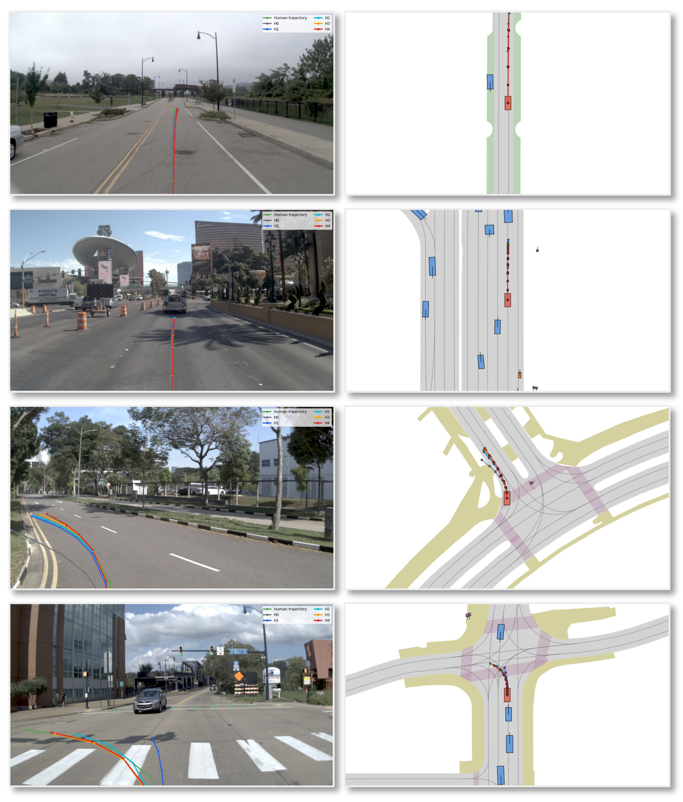
Figure A1 compares trajectories generated at different fixed rollout depths. In the first two simple lane-following scenes, predictions at all depths nearly overlap, indicating that additional rollout has little influence when the current observation already supports a stable plan. In contrast, the turning and intersection cases exhibit clear differences in trajectory curvature and direction across rollout depths. This comparison shows that sensitivity to rollout depth is scene-dependent: simple scenes remain stable across depths, whereas complex scenes require an appropriate rollout budget.
Figure A1.
Trajectory predictions at different fixed rollout depths. Predictions remain nearly identical in simple scenes but vary noticeably in turning and intersection cases.
Figure A1.
Trajectory predictions at different fixed rollout depths. Predictions remain nearly identical in simple scenes but vary noticeably in turning and intersection cases.
Appendix C.2. Latent Evaluator and Rollout Gate
Table A1 separates the contributions of the two Scheduler components. Adding the Latent Evaluator alone improves EPDMS/PDMS from 89.8/90.5 to 90.3/90.9, while the Gate alone raises them to 90.6/91.2. Combining both components gives the best result of 90.8/91.5, showing that evaluating predicted futures and adaptively allocating rollout provide complementary improvements.

Table A1.
Ablation of the Latent Evaluator and Rollout Gate on NAVSIM with all other components fixed.
Table A1.
Ablation of the Latent Evaluator and Rollout Gate on NAVSIM with all other components fixed.
| Latent Evaluator | Gate | EPDMS↑ | PDMS↑ |
|---|---|---|---|
| 89.8 | 90.5 | ||
| ✓ | 90.6 | 91.2 | |
| ✓ | 90.3 | 90.9 | |
| ✓ | ✓ | 90.8 | 91.5 |
Appendix C.3. Variable-Prefix Planner Training Distribution
Table A2 examines how the sampled prefix distribution affects variable-prefix Planner training. Uniform sampling performs best, while training only on the two extreme depths causes a substantial drop to 87.4 EPDMS. Short-heavy sampling remains competitive, but excluding the full prefix also degrades performance, indicating that balanced coverage of all valid depths is important.
Table A2.
Ablation of prefix-depth sampling for variable-prefix Planner training on NAVSIM. The distributions correspond to .
Table A2.
Ablation of prefix-depth sampling for variable-prefix Planner training on NAVSIM. The distributions correspond to .
| Strategy | Training Distribution | EPDMS↑ |
|---|---|---|
| Uniform | 89.8 | |
| Extremes | 87.4 | |
| Short-heavy | 89.6 | |
| No-full | 89.2 |
Appendix C.4. Number of Risk-Refinement Steps
As shown in Table A3, one refinement step already improves both metrics, and two steps increase PDMS/EPDMS from 90.5/89.8 to 90.9/90.2. Increasing m to 4 or 8 provides no further gain, so we use two steps to avoid redundant optimization.
Table A3.
Effect of the number of risk-refinement steps on NAVSIM.
| Steps m | PDMS↑ | EPDMS↑ |
|---|---|---|
| 0 | 90.5 | 89.8 |
| 1 | 90.7 | 90.1 |
| 2 | 90.9 | 90.2 |
| 4 | 90.9 | 90.2 |
| 8 | 90.9 | 90.2 |
Appendix C.5. Effect of the Computation-Cost Weight
Table A4 shows that a modest computation penalty improves EPDMS from 90.0 at to 90.8 at . Larger values substantially reduce planning performance, consistent with over-penalizing continued rollout. We therefore use as the default setting.
Table A4.
Effect of the computation-cost weight on NAVSIM planning performance.
| EPDMS↑ | |
|---|---|
| 0 | 90.0 |
| 0.001 | 90.7 |
| 0.005 | 90.8 |
| 0.01 | 88.6 |
| 0.05 | 88.4 |
Appendix D. Samples of CounterDrive
Figure A2.
Sample 1 of CounterDrive.
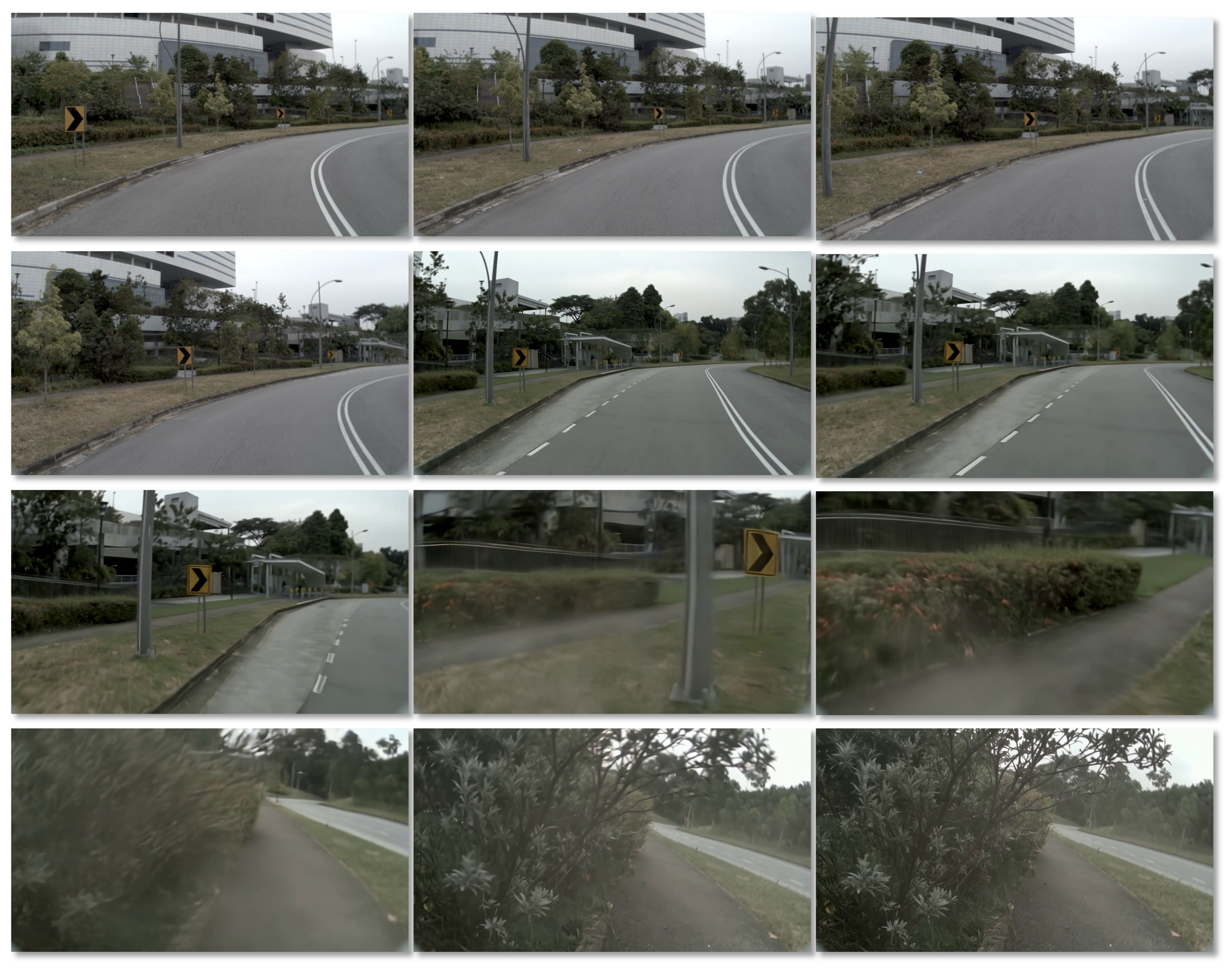
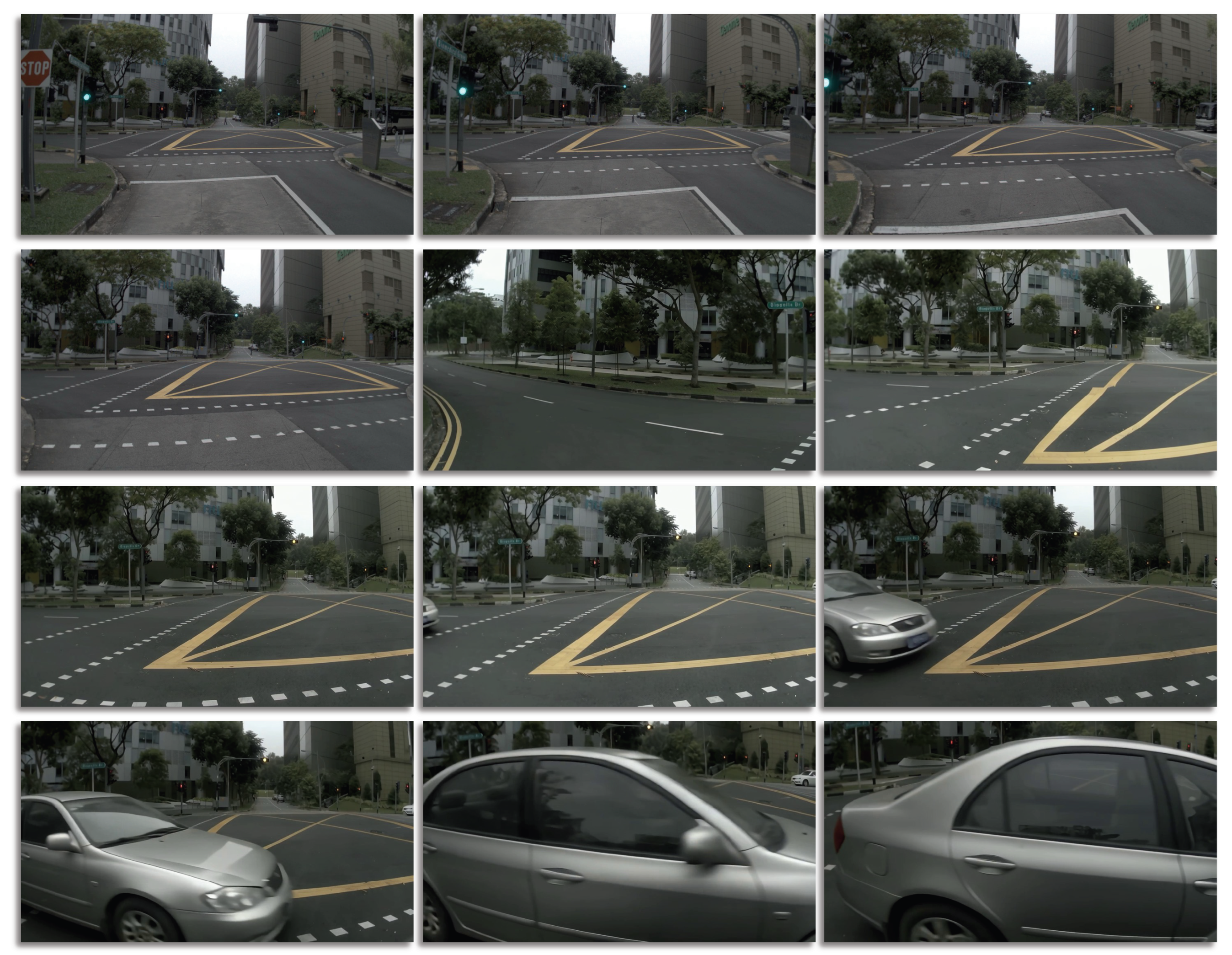
Figure A3.
Sample 2 of CounterDrive.
Appendix E. Prompts for CounterDrive Generation
CounterDrive constructs each video-generation prompt in two steps. First, a vision-language model (VLM) describes the near-field content of the source key frame and generates a one-sentence accident description. Second, these two variable components are concatenated with a manually written camera constraint prompt and supplied to Wan together with the source key frame. The operational prompts are written in Chinese; we provide faithful English translations below.
Appendix E.1. VLM-Based Prompt Construction
Table A5 presents the instructions used to generate the two variable prompt components. The key-frame description is restricted to nearby visible objects so that the subsequent accident description remains grounded in the source scene. The accident description explicitly specifies both the relative accident location and the involved object.
Table A5.
VLM instructions for constructing the variable components of the Wan prompt.
| Component | Prompt content and constraints |
|---|---|
| A. Near-field key-frame description | |
| VLM input | One front-facing dashcam key frame. |
| Role | You are a near-field object-description assistant for dashcam images. Given a front-facing dashcam image, describe only objects immediately surrounding the camera in exactly one sentence. Do not analyze accidents and do not describe the ego vehicle. |
| Spatial range | Only consider objects within approximately 30 m in front of the camera and 20 m on either side of the road. |
| Include | Include vehicles immediately ahead using their vehicle type only, such as “double-decker bus” or “SUV.” Also include nearby roadside objects, such as trees, guardrails, building facades, streetlights, or traffic signs. Mention the nearby road surface only when necessary. |
| Exclude | Do not mention city names, street names, distant landmarks, distant buildings, weather, illumination, time of day, detailed traffic conditions, or inferred geographical locations. |
| Output format | Return exactly one plain sentence. Do not output JSON, Markdown, numbering, explanations, or additional analysis. |
| Example output | “An SUV is immediately ahead, and a sedan is traveling in the adjacent left lane.” |
| B. Accident description | |
| VLM input | The source key frame and its near-field description generated in Part A. |
| Role | You are an accident-event description assistant for dashcam scenes. Based on the visible nearby objects, describe one physically plausible accident that occurs immediately after the source frame. |
| Grounding | Select an involved object that is visible in the key frame and present in the near-field description. Do not introduce a new vehicle, pedestrian, obstacle, or road structure. |
| Required content | Explicitly state the accident location relative to the ego vehicle, such as front, front-left, or front-right, and identify the involved object. Describe the event directly rather than analyzing its cause. |
| Temporal constraint | The accident must be a continuous and plausible evolution from the source key frame. Do not introduce camera cuts, viewpoint changes, or discontinuous object motion. |
| Output format | Return exactly one plain sentence. Do not provide reasoning, warnings, explanations, JSON, Markdown, or multiple candidate events. |
| Example output | “The ego vehicle directly rear-ends the SUV ahead.” |
Appendix E.2. Wan Video-Generation Prompt
The final Wan prompt contains three ordered components: a fixed camera prompt, the VLM-generated key-frame description, and the VLM-generated accident description. No additional language-model rewriting is applied after concatenation. Table A6 shows the template and an example.
Table A6.
Construction of the prompt supplied to Wan for counterfactual video generation.
| Component | Content |
|---|---|
| Wan input | The source key frame and the concatenated text prompt described below. |
| Fixed system prompt | “Dashcam perspective with fixed camera height and pitch. The camera height must remain unchanged, and no abrupt camera cuts may occur. The video must remain in a first-person driving view, and the ego vehicle must never appear in the image.” |
| Key-frame description | A one-sentence near-field scene description generated by the VLM using Part A of Table A5. |
| Accident description | A one-sentence accident description generated by the VLM using Part B of Table A5. The sentence specifies the accident location and involved object. |
| Concatenation rule | <FIXED CAMERA PROMPT> + <KEY-FRAME DESCRIPTION> +<ACCIDENT DESCRIPTION> |
| Complete example | “Dashcam perspective with fixed camera height and pitch. The camera height must remain unchanged, and no abrupt camera cuts may occur. The video must remain in a first-person driving view, and the ego vehicle must never appear in the image. An SUV is immediately ahead, and a sedan is traveling in the adjacent left lane. The ego vehicle directly rear-ends the SUV ahead.” |
| Wan output | A temporally continuous counterfactual driving video that preserves the source viewpoint and scene layout while realizing the specified accident. |
Appendix F. Algorithms of RISE
Appendix F.1. Inference
Here, RiskRefine denotes the iterative update in Eq. (A25) using the frozen Risk Profile branch of the Latent Evaluator; it is not a separate module.
| Algorithm A1: Adaptive inference with RISE |
| Require: Observation , observed ego-pose history , current ego kinematics , maximum horizon , computation preference |
| Ensure: Planned trajectory |
|
Appendix F.2. Training
| Algorithm A2: Three-stage training procedure of RISE |
| Require: Real data , accepted CounterDrive data , verified pair set , maximum horizon , and computation preferences |
| Ensure: Predictor , Planners , Latent Evaluator , and Rollout Gate |
| Stage I: Predictor and initial Planner |
|
References
- Li, K.; Li, Z.; Lan, S.; Xie, Y.; Zhang, Z.; Liu, J.; Wu, Z.; Yu, Z.; Alvarez, J.M. Hydra-mdp++: Advancing end-to-end driving via expert-guided hydra-distillation. arXiv preprint arXiv:2503.12820 2025.
- Shang, S.; Chen, Y.; Wang, Y.; Li, Y.; Zhang, Z. Drivedpo: Policy learning via safety dpo for end-to-end autonomous driving. arXiv preprint arXiv:2509.17940 2025.
- Chen, D.; Shukor, M.; Moutakanni, T.; Chung, W.; Yu, J.; Kasarla, T.; Bang, Y.; Bolourchi, A.; LeCun, Y.; Fung, P. Vl-jepa: Joint embedding predictive architecture for vision-language. arXiv preprint arXiv:2512.10942 2025.
- Maes, L.; Lidec, Q.L.; Scieur, D.; LeCun, Y.; Balestriero, R. Leworldmodel: Stable end-to-end joint-embedding predictive architecture from pixels. arXiv preprint arXiv:2603.19312 2026.
- Shen, Q.; Zhang, S.; Liao, Y.; Li, Q.; Tan, Z.; Wang, S.; Yan, S.; Wang, X. World Action Models: A Survey, 2026, [arXiv:cs.RO/2606.20781].
- Wang, S.; Shi, J.; Fu, Z.; He, X.; Liu, F.; Yang, C.; Zhou, Y.; Fei, Z.; Gong, J.; Fu, J.; et al. World Action Models: The Next Frontier in Embodied AI, 2026, [arXiv:cs.RO/2605.12090].
- Wang, L.; Yang, Z.; Bai, C.; Zhang, G.; Liu, X.; Zheng, X.; Long, X.X.; Lu, C.T.; Lu, C. Drive-JEPA: Video JEPA Meets Multimodal Trajectory Distillation for End-to-End Driving. arXiv preprint arXiv:2601.22032 2026.
- Yang, P.; Lu, B.; Xia, Z.; Han, C.; Gao, Y.; Zhang, T.; Zhan, K.; Lang, X.; Zheng, Y.; Zhang, Q. WorldRFT: Latent world model planning with reinforcement fine-tuning for autonomous driving. In Proceedings of the Proceedings of the AAAI Conference on Artificial Intelligence, 2026, Vol. 40, pp. 11649–11657.
- Wang, L.; Zheng, Y.; Chen, Q.; Li, S.; Zhang, Y.; Xing, Z.; Zhang, Q.; Li, X.; Qian, D.; Yang, P.; et al. Latent-WAM: Latent World Action Modeling for End-to-End Autonomous Driving, 2026, [arXiv:cs.CV/2603.24581].
- Yang, P.; Zheng, Y.; Qian, D.; Xing, Z.; Zhang, Q.; Wang, L.; Zhang, Y.; Guo, S.; Xia, Z.; Chen, Q.; et al. DreamerAD: Efficient Reinforcement Learning via Latent World Model for Autonomous Driving, 2026, [arXiv:cs.LG/2603.24587].
- Yuan, T.; Dong, Z.; Liu, Y.; Zhao, H. Fast-WAM: Do World Action Models Need Test-time Future Imagination? arXiv preprint arXiv:2603.16666 2026.
- Lu, H.; Yao, L.; He, C.; Wang, H.; Gu, X.; Li, X.; Liao, W.; He, T.; Peng, P. The DAWN of World-Action Interactive Models, 2026, [arXiv:cs.CV/2605.11550].
- Ha, D.; Schmidhuber, J. World models. arXiv preprint arXiv:1803.10122 2018, 2, 440.
- Zhou, G.; Pan, H.; LeCun, Y.; Pinto, L. Dino-wm: World models on pre-trained visual features enable zero-shot planning. arXiv preprint arXiv:2411.04983 2024.
- Li, S.; Gao, Y.; Sadigh, D.; Song, S. Unified Video Action Model, 2025, [arXiv:cs.RO/2503.00200].
- Kim, M.J.; Gao, Y.; Lin, T.Y.; Lin, Y.C.; Ge, Y.; Lam, G.; Liang, P.; Song, S.; Liu, M.Y.; Finn, C.; et al. Cosmos Policy: Fine-Tuning Video Models for Visuomotor Control and Planning, 2026, [arXiv:cs.AI/2601.16163].
- Li, L.; Zhang, Q.; Luo, Y.; Yang, S.; Wang, R.; Han, F.; Yu, M.; Gao, Z.; Xue, N.; Zhu, X.; et al. Causal World Modeling for Robot Control, 2026, [arXiv:cs.CV/2601.21998].
- Ye, S.; Ge, Y.; Zheng, K.; Gao, S.; Yu, S.; Kurian, G.; Indupuru, S.; Tan, Y.L.; Zhu, C.; Xiang, J.; et al. World Action Models are Zero-shot Policies, 2026, [arXiv:cs.RO/2602.15922].
- Team, M.; Xiang, C.; Bao, F.; Liu, H.; Tan, H.; Bi, H.; Li, J.; Liu, J.; Pang, J.; Jing, K.; et al. MotuBrain: An Advanced World Action Model for Robot Control, 2026, [arXiv:cs.RO/2604.27792].
- Yang, Y.; Liu, Z.; Kou, S.; Chen, Y.; Hu, Y.; Zhou, J.; Zhao, B.; Wei, Z.; Xia, X.; Li, X.; et al. World-Language-Action Model for Unified World Modeling, Language Reasoning, and Action Synthesis, 2026, [arXiv:cs.RO/2606.05979].
- Feng, T.; Wang, W.; Yang, Y. A Survey of World Models for Autonomous Driving, 2025, [arXiv:cs.RO/2501.11260].
- Yang, J.; Chitta, K.; Gao, S.; Chen, L.; Shao, Y.; Jia, X.; Li, H.; Geiger, A.; Yue, X.; Chen, L. Resim: Reliable world simulation for autonomous driving. Advances in Neural Information Processing Systems 2026, 38, 167710–167741.
- Hu, A.; Russell, L.; Yeo, H.; Murez, Z.; Fedoseev, G.; Kendall, A.; Shotton, J.; Corrado, G. Gaia-1: A generative world model for autonomous driving. arXiv preprint arXiv:2309.17080 2023.
- Wang, X.; Zhu, Z.; Huang, G.; Chen, X.; Zhu, J.; Lu, J. DriveDreamer: Towards Real-world-driven World Models for Autonomous Driving, 2023, [arXiv:cs.CV/2309.09777].
- Zheng, W.; Chen, W.; Huang, Y.; Zhang, B.; Duan, Y.; Lu, J. Occworld: Learning a 3d occupancy world model for autonomous driving. In Proceedings of the European conference on computer vision. Springer, 2024, pp. 55–72.
- Zhou, X.; Liang, D.; Tu, S.; Chen, X.; Ding, Y.; Zhang, D.; Tan, F.; Zhao, H.; Bai, X. Hermes: A unified self-driving world model for simultaneous 3d scene understanding and generation. In Proceedings of the Proceedings of the IEEE/CVF International Conference on Computer Vision, 2025, pp. 27817–27827.
- Liang, D.; Zhang, D.; Zhou, X.; Tu, S.; Feng, T.; Li, X.; Zhang, Y.; Du, M.; Tan, X.; Bai, X. Seeing the future, perceiving the future: A unified driving world model for future generation and perception. arXiv preprint arXiv:2503.13587 2025.
- Zhao, G.; Ni, C.; Wang, X.; Zhu, Z.; Zhang, X.; Wang, Y.; Huang, G.; Chen, X.; Wang, B.; Zhang, Y.; et al. Drivedreamer4d: World models are effective data machines for 4d driving scene representation. In Proceedings of the Proceedings of the computer vision and pattern recognition conference, 2025, pp. 12015–12026.
- Zhang, K.; Tang, Z.; Hu, X.; Pan, X.; Guo, X.; Liu, Y.; Huang, J.; Yuan, L.; Zhang, Q.; Long, X.X.; et al. Epona: Autoregressive diffusion world model for autonomous driving. In Proceedings of the Proceedings of the IEEE/CVF International Conference on Computer Vision, 2025, pp. 27220–27230.
- Hong, Y.; Zhou, X.; Li, Y.; Zhou, X.; Liu, L.; Luo, Y.; Xu, S.; Yang, L.; Song, Z. DriveFuture: Future-Aware Latent World Models for Autonomous Driving, 2026, [arXiv:cs.CV/2605.09701].
- Nguyen, P.; Nhu, A.N.; Lin, M.C. OpenVO: Open-World Visual Odometry with Temporal Dynamics Awareness. In Proceedings of the Proceedings of the IEEE/CVF Conference on Computer Vision and Pattern Recognition, 2026, pp. 14208–14218.
- Assran, M.; Bardes, A.; Fan, D.; Garrido, Q.; Howes, R.; Muckley, M.; Rizvi, A.; Roberts, C.; Sinha, K.; Zholus, A.; et al. V-jepa 2: Self-supervised video models enable understanding, prediction and planning. arXiv preprint arXiv:2506.09985 2025.
- Lu, C.; Zhou, Y.; Bao, F.; Chen, J.; Li, C.; Zhu, J. Dpm-solver++: Fast solver for guided sampling of diffusion probabilistic models. Machine Intelligence Research 2025, 22, 730–751.
- Xia, T.; Li, Y.; Zhou, L.; Yao, J.; Xiong, K.; Sun, H.; Wang, B.; Ma, K.; Chen, G.; Ye, H.; et al. DriveLaW:Unifying Planning and Video Generation in a Latent Driving World, 2026, [arXiv:cs.CV/2512.23421].
- Xu, J.; Zhong, Z.; Shu, Z.; Jia, M.; Li, M.; Bian, J.W.; Zhang, Q.; Zhang, K.; Xie, J.; Yang, J.; et al. EponaV2: Driving World Model with Comprehensive Future Reasoning, 2026, [arXiv:cs.CV/2605.14696].
- Chen, Y.; Wang, Y.; Zhang, Z. DrivingGPT: Unifying Driving World Modeling and Planning with Multi-modal Autoregressive Transformers, 2024, [arXiv:cs.CV/2412.18607].
- Li, Y.; Fan, L.; He, J.; Wang, Y.; Chen, Y.; Zhang, Z.; Tan, T. Enhancing end-to-end autonomous driving with latent world model. arXiv preprint arXiv:2406.08481 2024.
- Zheng, Y.; Yang, P.; Xing, Z.; Zhang, Q.; Zheng, Y.; Gao, Y.; Li, P.; Zhang, T.; Xia, Z.; Jia, P.; et al. World4drive: End-to-end autonomous driving via intention-aware physical latent world model. In Proceedings of the Proceedings of the IEEE/CVF International Conference on Computer Vision, 2025, pp. 28632–28642.
- Li, Y.; Shang, S.; Liu, W.; Zhan, B.; Wang, H.; Wang, Y.; Chen, Y.; Wang, X.; An, Y.; Tang, C.; et al. DriveVLA-W0: World Models Amplify Data Scaling Law in Autonomous Driving, 2025, [arXiv:cs.CV/2510.12796].
- Zhao, Z.; Fu, T.; Wang, Y.; Wang, L.; Lu, H. From Forecasting to Planning: Policy World Model for Collaborative State-Action Prediction. arXiv preprint arXiv:2510.19654 2025.
Figure 1.
Comparison of various imagination strategies in WAMs. (a) Imagine and Plan jointly uses observed and predicted latents for planning, (b) Imagine then Plan performs future rollout before action generation, and (c) No Imagination plans directly from the observation. (d) RISE introduces a lightweight Scheduler that adaptively routes computation to further prediction or final planning.
Figure 1.
Comparison of various imagination strategies in WAMs. (a) Imagine and Plan jointly uses observed and predicted latents for planning, (b) Imagine then Plan performs future rollout before action generation, and (c) No Imagination plans directly from the observation. (d) RISE introduces a lightweight Scheduler that adaptively routes computation to further prediction or final planning.
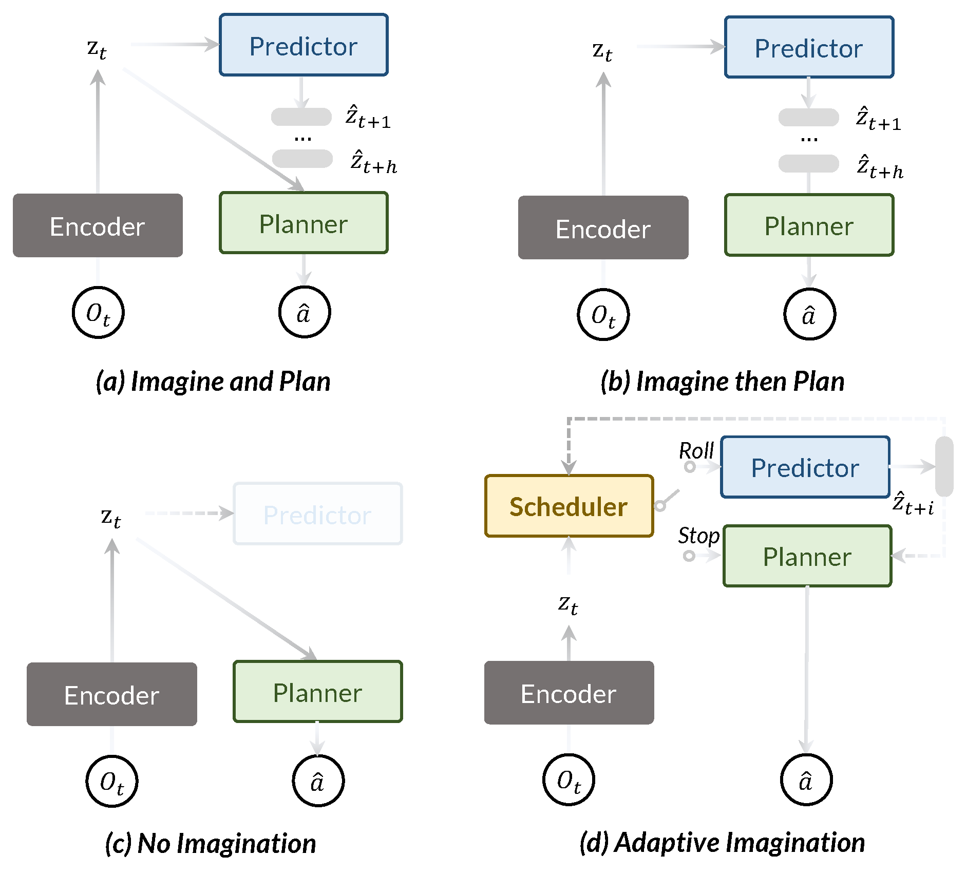
Figure 2.
Overview of RISE. The WAM learns future prediction and variable-prefix planning. The Latent Evaluator predicts a Risk Profile and a Future Planning Gain Profile , supervised by counterfactual risks and all-horizon planning outcomes. The Rollout Gate balances the predicted gain against computation cost, routing to further rollout and to planning.
Figure 2.
Overview of RISE. The WAM learns future prediction and variable-prefix planning. The Latent Evaluator predicts a Risk Profile and a Future Planning Gain Profile , supervised by counterfactual risks and all-horizon planning outcomes. The Rollout Gate balances the predicted gain against computation cost, routing to further rollout and to planning.
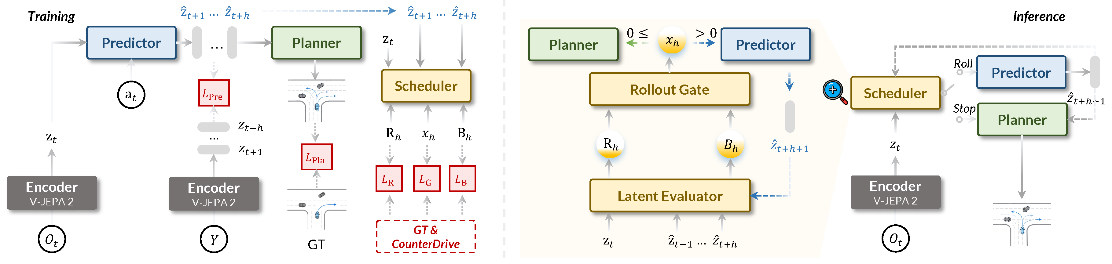
Figure 3.
Performance under different rollout depths.
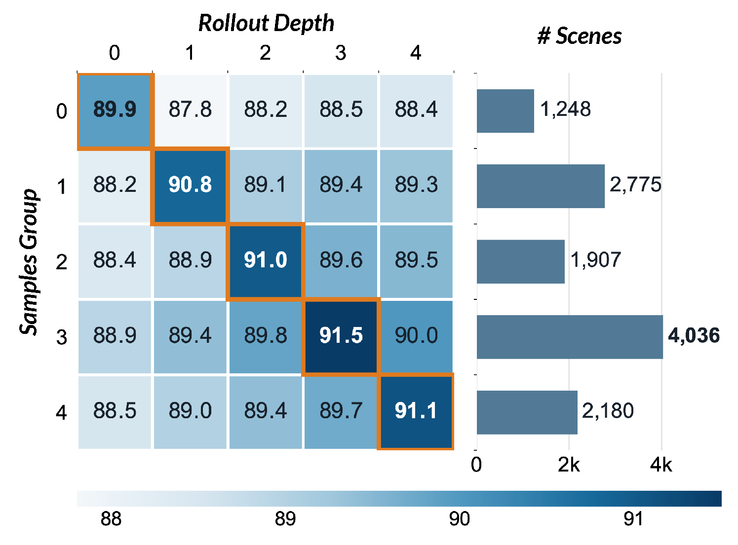
Figure 4.
Representative scenes grouped by their preferred rollout depths. Scenes with denser traffic and more involved interactions generally benefit from additional rollout.
Figure 4.
Representative scenes grouped by their preferred rollout depths. Scenes with denser traffic and more involved interactions generally benefit from additional rollout.
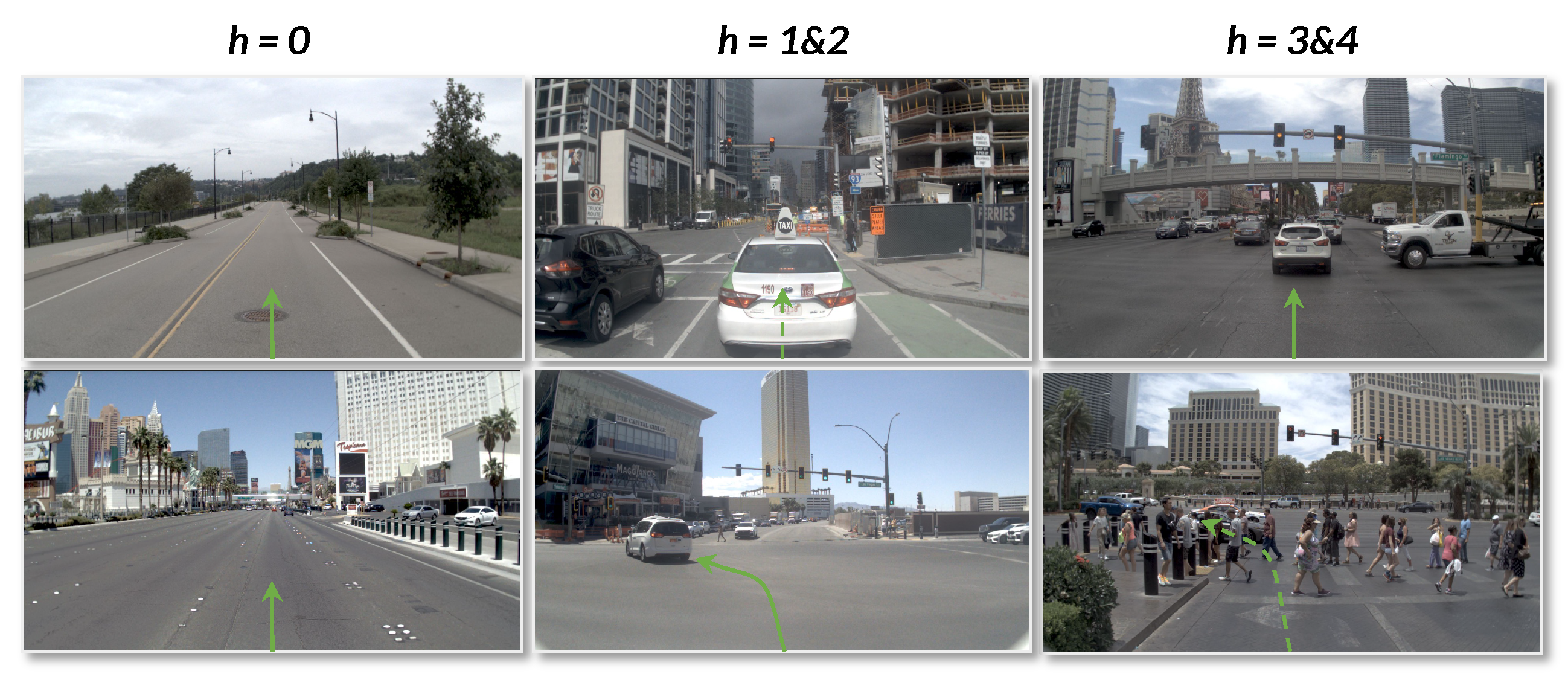
Figure 5.
Qualitative trajectory comparison on NAVSIM at depths to . The rows show front-camera views and corresponding bird’s-eye-view scenes. Human, Drive-JEPA, and RISE trajectories are shown in green, yellow, and red, respectively. RISE remains aligned with human trajectories and feasible lane geometry across scene-dependent rollout depths.
Figure 5.
Qualitative trajectory comparison on NAVSIM at depths to . The rows show front-camera views and corresponding bird’s-eye-view scenes. Human, Drive-JEPA, and RISE trajectories are shown in green, yellow, and red, respectively. RISE remains aligned with human trajectories and feasible lane geometry across scene-dependent rollout depths.
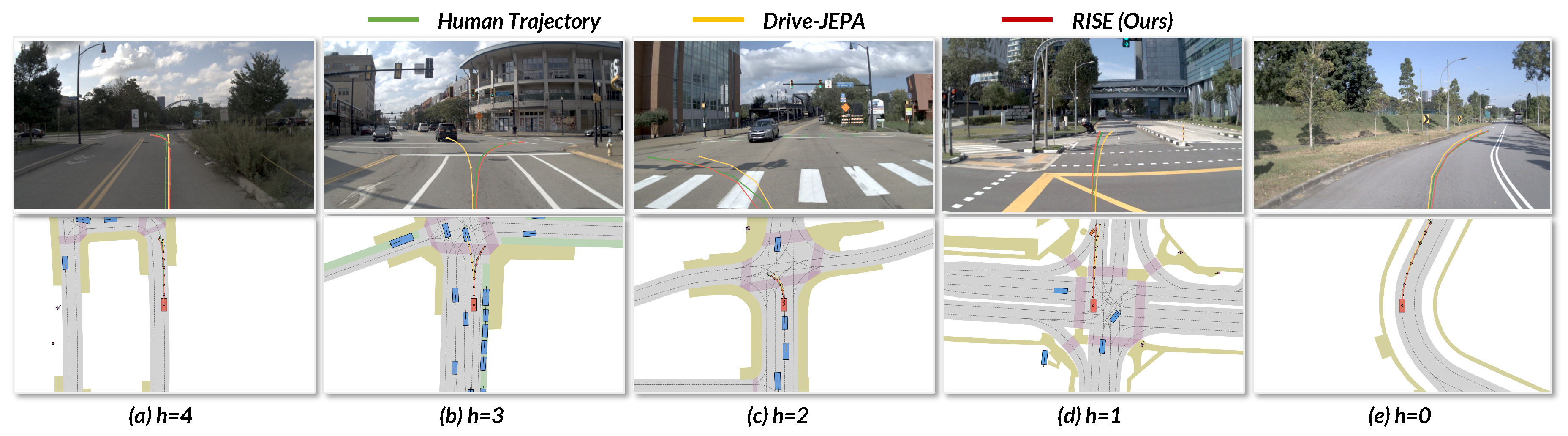
Table 1.
Performance on nuScenes.
| Method | L2 (m)↓ | Collision Rate↓ | ||||||
|---|---|---|---|---|---|---|---|---|
| 1s | 2s | 3s | Avg. | 1s | 2s | 3s | Avg. | |
| BEV-Planner | 0.30 | 0.52 | 0.83 | 0.55 | 0.10 | 0.37 | 1.30 | 0.59 |
| LAW | 0.26 | 0.57 | 1.01 | 0.61 | 0.14 | 0.21 | 0.54 | 0.30 |
| World4Drive | 0.23 | 0.47 | 0.81 | 0.50 | 0.02 | 0.12 | 0.33 | 0.16 |
| WorldRFT | 0.21 | 0.44 | 0.76 | 0.47 | 0.10 | 0.11 | 0.23 | 0.15 |
| DAWN | 0.17 | 0.31 | 0.52 | 0.33 | 0.00 | 0.10 | 0.23 | 0.11 |
| RISE | 0.16 | 0.29 | 0.49 | 0.31 | 0.00 | 0.11 | 0.20 | 0.10 |
Table 2.
Performance on NAVSIMv1.
| Method | NC↑ | DAC↑ | EP↑ | C↑ | TTC↑ | PDMS↑ |
|---|---|---|---|---|---|---|
| DrivingGPT | 98.9 | 90.7 | 79.7 | 95.6 | 94.9 | 82.4 |
| LAW | 97.4 | 93.3 | 78.8 | 100 | 91.9 | 83.8 |
| World4Drive | 97.4 | 94.3 | 79.9 | 100 | 92.8 | 85.1 |
| Epona | 97.9 | 95.1 | 80.4 | 99.9 | 93.8 | 86.2 |
| DriveVLA-W0 | 98.4 | 95.3 | 80.9 | 100 | 95.2 | 87.2 |
| PWM | 98.6 | 95.9 | 81.8 | 100 | 95.4 | 88.1 |
| DreamerAD | 98.0 | 97.2 | 83.1 | 100 | 94.3 | 88.7 |
| DriveLaW | 99.0 | 97.1 | 81.3 | 100 | 96.7 | 89.1 |
| Drive-JEPA | 98.7 | 96.2 | 82.9 | 100 | 95.5 | 89.0 |
| DAWN | 98.7 | 95.9 | 84.3 | 100 | 96.0 | 89.1 |
| EponaV2 | 98.6 | 97.9 | 84.8 | 100 | 95.7 | 90.4 |
| DriveFuture | 98.8 | 99.1 | 95.4 | 100 | 84.2 | 90.7 |
| RISE | 99.1 | 97.7 | 98.3 | 100 | 98.6 | 91.5 |
Table 3.
Performance on NAVSIMv2.
| Method | NC↑ | DAC↑ | DDC↑ | TL↑ | EP↑ | TTC↑ | LK↑ | HC↑ | EC↑ | EPDMS↑ |
|---|---|---|---|---|---|---|---|---|---|---|
| DAWN [12] | 97.3 | 92.0 | 99.1 | 99.7 | 87.4 | 96.6 | 96 | 98.3 | 85.5 | 83.2 |
| DreamerAD [10] | 98.0 | 97.2 | 99.5 | 99.8 | 87.8 | 97.4 | 97.5 | 98.3 | 72.4 | 85.1 |
| DriveLaW [34] | 98.7 | 96.9 | 99.6 | 99.8 | 87.5 | 98.3 | 97.6 | 98.4 | 77.4 | 88.6 |
| EponaV2 [35] | 98.5 | 97.4 | 99.5 | 99.9 | 87.9 | 98.1 | 97.7 | 98.2 | 77.4 | 88.9 |
| Latent-WAM [9] | 98.1 | 97.3 | 99.6 | 99.8 | 87.7 | 97.3 | 97.6 | 98.1 | 87.3 | 89.3 |
| DriveFuture [30] | 98.8 | 99.1 | 99.6 | 99.9 | 86.6 | 98.4 | 96.4 | 98.3 | 74.8 | 89.9 |
| RISE | 99.1 | 97.7 | 99.7 | 99.9 | 87.8 | 98.7 | 98.0 | 98.4 | 87.4 | 90.8 |
Table 4.
Ablation of the Scheduler and CounterDrive on NAVSIM. Both components improve performance.
| Scheduler | CounterDrive | EPDMS↑ | PDMS↑ |
|---|---|---|---|
| 88.9 | 89.7 | ||
| ✓ | 89.8 | 90.5 | |
| ✓ | 90.4 | 91.2 | |
| ✓ | ✓ | 90.8 | 91.5 |
Table 5.
Ablations on different adaptive rollout strategies. Random Stop stops at a random horizon from 0 to 4, while Latent Margin stops when consecutive latents converge.
Table 5.
Ablations on different adaptive rollout strategies. Random Stop stops at a random horizon from 0 to 4, while Latent Margin stops when consecutive latents converge.
| Method | # Avg. Rollout | Latency (ms) | EPDMS↑ |
|---|---|---|---|
| Random Stop | 2.03 | 264.075 | 89.5 |
| Latent Margin | 2.98 | 308.532 | 89.7 |
| Scheduler | 2.40 | 287.429 | 90.8 |
Table 6.
Effect of CounterDrive on safety-critical evaluation. AUC@h measures hazard–safe risk ranking at horizon h. Acc measures accident recognition.
Table 6.
Effect of CounterDrive on safety-critical evaluation. AUC@h measures hazard–safe risk ranking at horizon h. Acc measures accident recognition.
| CounterDrive | AUC↑ | Acc↑ | |||
|---|---|---|---|---|---|
| @1s | @2s | @3s | @4s | ||
| 0.49 | 0.52 | 0.51 | 0.50 | 0.51 | |
| ✓ | 0.96 | 0.95 | 0.96 | 0.93 | 0.96 |
Table 7.
Transfer of the RISE Scheduler to DAWN. Adding the Scheduler consistently improves planning performance without modifying the underlying WAIM.
Table 7.
Transfer of the RISE Scheduler to DAWN. Adding the Scheduler consistently improves planning performance without modifying the underlying WAIM.
| Method | NC↑ | DAC↑ | EP↑ | C↑ | TTC↑ | PDMS↑ |
|---|---|---|---|---|---|---|
| DAWN | 98.7 | 95.9 | 84.3 | 100 | 96.0 | 89.1 |
| + Scheduler | 99.9 | 96.8 | 87.0 | 100 | 98.3 | 90.3 |
Disclaimer/Publisher’s Note: The statements, opinions and data contained in all publications are solely those of the individual author(s) and contributor(s) and not of MDPI and/or the editor(s). MDPI and/or the editor(s) disclaim responsibility for any injury to people or property resulting from any ideas, methods, instructions or products referred to in the content. |
© 2026 by the authors. Licensee MDPI, Basel, Switzerland. This article is an open access article distributed under the terms and conditions of the Creative Commons Attribution (CC BY) license (http://creativecommons.org/licenses/by/4.0/).
Copyright: This open access article is published under a Creative Commons CC BY 4.0 license, which permit the free download, distribution, and reuse, provided that the author and preprint are cited in any reuse.