

Submitted:
17 August 2026
Posted:
19 August 2026
You are already at the latest version
Abstract
An involution of an exceptional geometry of type E7 is called regular if its fix structure, viewed as simplicial complex, is a building. Involutions which do not act trivial on the underlying field correspond to Galois descent and were treated a long time ago by Jacques Tits. In the present paper, we classify the regular involutions of geometries of type E7 that act trivial on the underlying (arbitrary) field, which we assume not to have characteristic 2. As a result, we discover new subgeometries of the exceptional geometry of type E7.
Keywords:
spherical buildings
; involution
; exceptional type E7
; generalised quadrangles
; metasym-plectic space
; Moufang set
MSC: 51E24
1. Introduction
Involutions play a prominent and important role in both algebra and geometry. For instance, centralisers of involutions in known groups gave rise to new simple groups, cf. the simple Suzuki and Ree groups. Also, involutions in geometries usually give rise to interesting and large subgeometries, for instance Baer subspaces of projective spaces. These two examples connect in the theory of Tits buildings with each other by considering an involution in a spherical building: its centraliser may well be a simple algebraic group acting on the (large) fix structure, which is a spherical building itself.
In the present paper, we determine all fix structures of linear involutions of spherical buildings of exceptional type that do not pointwise fix an apartment (or, equivalently, a chamber; see below for the motivation), and as a corollary we find a lot of simple algebraic groups inside the one of type which were not realised before. Since the root system of type is a subsystem of the root system of type , it does not come as a big surprise that forms of type turn up and play a central role. Recall that a linear involution is one that acts trivially on the underlying field. The non-linear involutions give rise to Galois descent, which is described in detail in [32]. The motivation of our restriction to involutions not fixing a chamber is mainly the analogy with Galois descent: each descent group corresponds to a Tits index (which can be viewed as a fix diagram) which determines the type and a thick spherical subbuilding of that type. If one fixes a chamber, then, in the linear case, the fix structure is never a thick subbuiding, and the type of the thick frame is not determined by the fix diagram. If a linear involution does not fix a chamber, then we will see that in all but one cases the fix diagram describes the type of the thick fix subbuilding unambiguously. A second reason is that the study of involutions fixing a chamber requires different methods, and this shall be done elsewhere. One preliminary result in that direction is that the “thick frame” of the fixed building of an involution that pointwise fixes an apartment is always split, that is, it admits a so-called “full” Tits index. This is automatic for buildings of simply laced type defined over a commutative field. In case of buildings of type , buildings of type and turn up.
Let be a geometry of type , defined over an arbitrary field of characteristic not 2. To each involution of is associated its fix geometry, that is, the geometry of the fixed vertices. The fix diagram encodes these types. The principal goal of the paper is to classify all linear involutions of according to their fix diagrams, when the latter is not full, that is, not all types admit fixed vertices. In particular we prove that each fix geometry is the geometry associated to a spherical building itself (possibly of rank 1, or even 0) and we provide an explicit list of all possibilities through their description/definition via Galois descent and the corresponding Tits index. If the geometry is empty, then we prove that the involution is anisotropic, that is, maps each simplex to an opposite simplex, and we also determine the imaginary fix building, yielding the (type of the) centraliser of the given involution.
Let us also mention that the case of type is particularly interesting since it allows the most number of Tits indices and fix diagrams for involutions among all exceptional types. This implies for instance that, in contrast to all other exceptional types, there are buildings of rank 3 which are the fix structure of an involution in a building of type . See Figure 1 for the enumeration of all possible fix diagrams for involutions of a building of type .
Motivation
The absolute geometry of a linear involution is in general larger than the one of a non-linear involution. So, our classification in particular exhibits relatively large subgeometries of geometries of type . This contributes to our knowledge of the structure of such geometries, just like the subgroup structure of a group provides very useful information. Moreover, the centralisers of the involutions are large subgroups of the groups of type and our results contribute to the subgroup structure of those groups.
Let us finally mention that the assumption of characteristic not equal to 2 is necessary, as in characteristic 2, linear involutions behave completely different. In particular, there are linear involutions not fixing any chamber but yet their fix structure is not a subbuilding. This requires other, additional methods and shall be done elsewhere.
Structure of the Paper
In Section 2, we introduce the necessary notions in order to be able to state our main results more precisely. Then, in Section 3, we recall some known results that we will use in our proofs. Most of them will concern the standard exceptional geometry of type over an arbitrary field , which fully describes the corresponding building of type . Our method requires some knowledge about involutions in two other types of geometries: projective spaces and hyperbolic quadrics in projective spaces of dimension at most 11. We study the latter in Section 4. Then, in Section 5 we prove our main results. The last section is devoted to examples, which should also settle existence of the different classes of involutions turning up in our main result.
Section 2 and Section 3 contains some overlap with [8], as the goals and background of the latter are very similar to those of the present paper. Instead of referring, we rather repeat for the convenience of the reader.
This paper grew out of the master thesis of the first author, written under the supervision of the second author at Ghent University, academic year 2025–2026.
2. Main Result
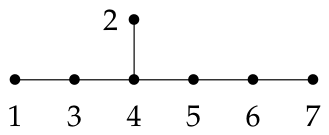
We assume the reader is familiar with the basics of (spherical) building theory, see [1,33], in particular with opposition, Coxeter and Dynkin diagrams and the Moufang condition. We will view a spherical building as a simplicial complex, numbering the types of the vertices with Bourbaki labeling [9]. In the present paper, we are concerned with buildings of type . Their symmetric Coxeter or Dynkin diagram, including the Bourbaki labeling, looks like
It is proved in [33] that for each field , there exists a unique building of type , which we denote by , and call the building of type over . The latter is sometimes also referred to as the ground field. It means that each projective space that turns up as a residue is defined using a vector space over .
In order to state our main results, we need terminology and notation to describe the fix geometry of an involution within , and its abstract isomorphism type within the world of spherical buildings. We will do so with the help of fix diagrams and Tits indices. The former, being more intuitive than the latter, helps to better understand the latter.
2.1. Fix Diagrams
Let be an arbitrary irreducible spherical building, and let G be an automorphism group of . Then the fix diagram for G is the Coxeter/Dynkin diagram of furnished with encircled orbits of nodes under the action of G on the diagram indicating the types of minimal simplices that are fixed by G. Note that, as soon as G preserves types and fixes a chamber, which is somehow the generic case, the fix diagram is trivial—all nodes are encircled. But in this case, the fix diagram obviously does not provide useful information. However, if the fix structure is a building again, then such diagrams are very useful, and we will only use fix diagrams in that case. Some examples related to are given in Figure 1, where we also introduce the names of the various fix diagrams, for later reference.
Fix diagrams in which each node is separately encircled are called full, e.g. .
2.2. Tits Indices
Tits indices are introduced in [32], and therein called simply indices, as a generalisation of the classical Witt index. They can be considered as a special case of a fix diagram in the following way. Recall that each simple algebraic group G gives rise to a unique irreducible spherical building , see chapter 5 of [33]. Now let G be defined over an algebraically closed field . Let be an automorphism group of . Denote the fixed field by . Note that is a Galois group for the extension . Then one can let act on G as an outer automorphism group. The fixed point group—also called the group of rational points in the literature—is a simple algebraic group H over . The spherical building arises from as the fix structure of the group . The corresponding Tits index is the fix diagram furnished with some other data regarding the algebraic groups, such as dimensions of anisotropic kernels and the like, see [32]. Since for our purposes, it is enough to understand the connection with fix diagrams, we refer to [32] for more precise information. We note that, if a spherical building arises from a Tits index, then the latter is unique for the building. A building is called split if it arises from a Tits index which is full as a fix diagram. Written in the symbols of [32] the Tits index is then of the form , if , and , if . For instance, every building of type is split, as follows from the tables in [32]. The type of the building is called the absolute type of , whereas the actual type of is sometimes referred to as the relative type. We say that arises from by Galois descent.
2.3. Moufang Buildings
Although we will not need a formal definition, it is instructive to mention the notion of a Moufang (spherical) building. This is a spherical building whose automorphism group satisfies certain transitivity properties, see [33, Addendum]. All spherical buildings of rank at least 3 are Moufang and they arise either from Galois descent, or from a classical group, or from a group of mixed type . This is explained in [34]. However, in rank 2, there are exotic examples of buildings. Rank 2 simplical complexes are just graphs and irreducible thick spherical buildings of rank 2 are graphs with diameter n and girth , , without vertices of valency 2. These are the thick generalised n-gons. The Moufang condition [35] distinguishes the exotic ones from the ones that behave just like the higher rank irreducible spherical buildings. For instance, the Moufang rank 2 buildings also arise either from Galois descent, or from a classical group, or from groups of mixed type or . We note that some Moufang buildings can arise both from Galois descent and from a classical group. A group of mixed type is a phenomenon in low characteristic using purely inseparable field extensions. It only applies to buildings of type and in characteristic 2 and type in characteristic 3.
The importance of the Moufang condition for the present paper is that, if the fix structure of an involution is a building, then it is a Moufang building, see [24, Theorem 24.31]. Hence the fixed building either arises from Galois descent, or from a classical group, of from a group of mixed type. In our cases, it will always arise from Galois descent.
2.4. Preview of the Main Results
Finally, before stating our main result, we discuss the way we present it. Our theorem contains information about different types of linear involutions of buildings of type . This information is given in tabular form. For a given involution, we provide two data. The first one is the fix diagram, as discussed in Section 2.1. This explains how the fix structure sits into the ambient building of type by revealing which types of simplices are fixed. The second one is the Tits index. This provides the abstract isomorphism type of the fixed building as explained above in Section 2.2. In one case, the fixed building has rank 1, which we did not yet discuss. In that case, [24, Theorem 24.31] asserts that the fixed building is a Moufang set, as defined and discussed by Tits in [34]. The ones that we will encounter will all arise from Galois descent, and hence, again, they correspond to Tits indices. In a final case, the fixed building is empty, in other words, the involution is anisotropic. In this case we mention the type of the imaginary fix building, that is, the building seen over a suitable field extension.
2.5. Main Result
We can now state our main result. We assign each class of involutions a type for further reference.
Theorem A.
Let Δ be a building of type over a field with . Let ρ be a linear involution of Δ, Suppose ρ is not anisotropic, that is, it maps at least one object not to an opposite object. Then its fix structure is a building (possibly of rank 1) and, if ρ does not pointwise fix an apartment, then the associated fix diagram and corresponding Tits index are given as in Figure 2. Along with the diagram, we mention the name of the corresponding fix diagram. We add a column with the name and symbol of the Tits index as introduced by in [32].
2.6. Some More Discussion
It is interesting to note that almost all absolute types of the fix structures are , and almost all possible Tits indices of the latter occur. As mentioned in the introduction, this has to do with the fact that the root system of type is a subsystem of the root system of type (and no other subsystem of roots is irreducible and has rank 7).
Let us mention once again that Tits [32] studied the case of non-linear involutions. The related Tits indices correspond to the fix diagrams given in Figure 1 and are and . So our paper can be considered as a complement to these results.
As already mentioned, we refer to Section 6 for (the construction of) examples. There, it will become clear which properties a field needs to have in order to admit a regular involution of a given type. Here we mention that over a finite field, only involutions of types I and II exist, and over the real numbers, only Types I up to IV, and VII occur. Over the complex numbers, as well as over any algebraically closed field, every linear involution fixes a chamber as follows from the Density Theorem.
3. Preliminaries
3.1. Buildings and Point-Line Geometries
As already mentioned, we assume familiarness with the basic notions in the theory of spherical buildings. We also use the standard notation such as for the residue in the building of the element x (sometimes omitting from this notation if no ambiguity can arise). We say that an automorphism is anisotropic if it maps every simplex to an opposite simplex. We have the following characterisation of anisotropic automorphisms. It basically says that it suffices to look at the images of vertices of any given type in order to check whether an automorphism is anisotropic or not.
Lemma 3.1
(Theorem 3.1 of [19]). An automorphism of a spherical building maps every element of a given type to an opposite element if, and only if, it is anisotropic.
The way we are going to approach buildings in this paper is via their most standard geometry. More precisely, we turn them into point-line geometries using a well known recipe. Before quickly describing that recipe, we define point-line geometries.
Definition 3.2.
A point-line geometry is a bipartite graph where the vertices of a given class X are called points and the vertices of the other class Y are called lines. Points adjacent to a common line are called collinear and we denote . The set of points collinear to a given point x is denoted as . A repeated line is a set of points that is the neighbourhood of two distinct lines. A subgeometry is an induced subgraph, and it is called full if it contains the full neighbourhood in of any of its lines. A subgeometry is called convex if it contains all vertices of each shortest path between every pair of its vertices. A subgeometry is called a geometric hyperplane if for each line L, the neighbour set either is contained in it, or intersects the subgeometry in a unique point.
For a given point-line geometry with classes X and Y, we define . Then the bipartite graph with classes X and , where a point is adjacent to any member L of containing x, is a point-line geometry without repeated lines. We call the reduction of . The graph is completely determined by the sets X and .
Definition 3.3.
Now let be an irreducible spherical building. Recall that, for the type set, we always use the Bourbaki labeling [9] of vertices of the corresponding diagram. Let X be the set of vertices of some given type, say i. Define Y to be the set of panels of cotype i. A vertex v of type i is adjacent to a panel P of cotype i if is a chamber. This defines a point-line geometry the reduction of which is called the i-Grassmannian of . If the diagram of is simply laced, and has rank , then is determined by its diagram, say , and a given skew field . In that case we denote by and its i-Grassmannian by . In general, we say that Γ is a Lie incidence geometry of type .
3.2. Projective Spaces
With the conventions of Theorem 3.3, the projective space of dimension n over a skew field , which is usually denoted , is also denoted by . Projective planes are Lie incidence geometries of type . A collineation of is a permutation of the point set preserving the line set. An involution is a collineation of order 2. A duality is an automorphism of the underlying building that, using the usual Bourbaki labelling [9], interchanges the types i and . A polarity is a duality of order 2.
We will need the following two lemmas for projective spaces.
Lemma 3.4.
An involution of a projective space of even dimension fixes at least one point. An involution of a projective plane fixes at least three points and at least three lines.
Proof.
The next lemma immediately follows from [27, Proposition 3.3].
Lemma 3.5.
Let σ be an involution of , , . Suppose σ is induced by a linear transformation of the underlying vector space.
- 1.
- Suppose that either d is even, or σ admits at least one fixed point. Then the set of fixed points is the union of two disjoint subspaces U and , with .
- 2.
- Suppose that d is odd and σ does not fix any point. Then σ fixes a spread of lines elementwise, that is, it globally stabilises a line through each point.
We also introduce the following notation: for a set S of points of a projective space, we denote by the projective subspace generated by the elements of S.
3.3. Hyperbolic Quadrics
In the present paper, we will approach buildings of type mainly via their Lie incidence geometries of type . An important ingredient to define such geometries and list their properties is the notion of a hyperbolic quadric and the related building of type , for some natural .
Definition 3.6.
A hyperbolic quadric Q (over the field is the set of points of a projective space , , whose coordinates with respect to a suitable basis, satisfy the quadratic equation
where we work with generic coordinates . If , then such a quadric also arises from a polarity of by collecting the absolute elements, that is, the subspaces U of contained in their own image under . The maximum (projective) dimension of subspaces entirely contained in Q is , and such subspaces are called generators. They fall into two classes in such a way that subspaces belonging to distinct classes intersect each other in a projective subspace of dimension , with i even. We call these classes the oriflamme classes. Subspaces contained in Q are usually called singular subspaces. The vertices of the corresponding building of type are the singular subspaces of projective dimension , and the maximal singular subspaces comprise two types of vertices according to the oriflamme class they are contained in. Two vertices corresponding to singular subspace of dimension form a simplex if they intersect in a subspace of dimension (see [33]). A duality of is a collineation of preserving Q and interchanging the two oriflamme classes. As usual, a polarity is a duality of order 2.
Note that the points and lines of Q define the geometry .
In general, quadratic equations define quadrics, and the Witt index of a quadric is one more than the maximum projective dimension of a singular subspace. A quadric is non-degenerate if there exist disjoint maximal singular subspaces. A non-degenerate quadric of Witt index n
- 1.
- in is called a parabolic quadric;
- 2.
- in is called an elliptic quadric;
- 3.
- in , , is called a hyperelliptic quadric.
We have the following property of involutions and polarities in , ..
Lemma 3.7.
Every polarity ρ of a hyperbolic quadric , , fixes at least one point. Every type-preserving involution ρ of a hyperbolic quadric , , fixes at least one point.
Proof.
Let U be an arbitrary maximal singular subspace. Then either is a point (which is fixed under ), or is a projective space of even dimension. In the latter case induces an involution in . Then the result follows from Theorem 3.4. □
3.4. Geometries of Type .
Now let be a building of type over the field . We are going to work with the Lie incidence geometry , the 7-Grassmannian of , denoted by , and with , the 1-Grassmannian of , denoted by . The respective sets of symps are denoted as and . A good reference is [17], see also the later chapters of [28]. Additional properties of will be derived using an apartment of the corresponding building (since every pair of chambers are contained in an apartment, this method will be especially efficient when a property only involves two simplices). We gather them in this preliminary section as they are independent of an involution. This way they do not interrupt the flow of the proof of the main results in Section 4 and Section 5.
We begin with describing the elements of and linking them to the Coxeter diagram. The points of are the vertices of type 7 of the building , by the very definition. The lines correspond to the vertices of type 6. Vertices of type 5 are planes of , whereas vertices of type 4, 3 and 2 are projective subspaces of dimension 3, 5 and 6, respectively. We refer to them as 3-spaces, 5-spaces and 6-spaces, respectively. Finally, vertices of type 1 correspond to convex subspaces of isomorphic to and will be called symplecta, or briefly symps, as in the theory of parapolar spaces. But we avoid introducing the latter theory here, and refer instead to the later chapters of [28].
We display the basic properties of (which can be found in [17]).
Proposition 3.8.
Let be two points of and let be two symps. Then the following properties hold.
- (i)
- Either , or there is a unique line containing both x and y, or x and y are not collinear and there is a unique symp containing both x and y, or no symp contains both x and y;
- (ii)
- Either , or x is contained in unique 6-space which intersects ξ in a maximal singular subspace distinct from a 5-space, or x is collinear to a unique point of ξ (in the latter case we refer to this situation as x being far from ξ);
- (iii)
- Either , or is a 5-space (we then call them adjacent), or is a line, or and there is a unique symp adjacent to both ξ and ζ, or and every point of ξ is far from ζ and vice versa.
The intersection of the unique 6-space in with the symp will be referred to as a -space. It follows from considering the diagram of type that 5-spaces and -spaces of a symp belong to different oriflamme classes. The unique symp through x and y in is sometimes denoted as .
Definition 3.9.
As already mentioned in the propositions, two symps of are called adjacent if they intersect in a 5-space. A point x and a symp are called far if exactly one point of is collinear to x; they are called close if x is collinear to a -space of .
In fact, the properties in Theorem 3.8 can easily be checked inside an apartment, keeping in mind that every pair of simplices is contained in a common apartment. We now present an explicit construction of such an apartment , based on [22], and we call it the standard apartment. Set , . The point set of is
Let be the set of members of S or size 2 and those of size 6. Lines, or vertices of type 6, in are the pairs
This defines a graph . The vertices of types 5, 4 and 2 correspond to the cliques of size 3, 4 and 7, respectively, those of type 3 to the maximal cliques of size 6, and those of type 1 to the so-called hexacrosses, which are induced subgraphs isomorphic to a clique of size 12 minus a perfect matching. The latter is an apartment of a building of type . There are two kinds of hexacrosses in this description: those that consist of the elements of contained in a given 4-set T of and the elements of containing T; ands those that, for a given ordered pair , , consist of the members of containing i but not j.
Let us for instance check Theorem 3.8. As symp we can take the set of vertices, with obvious shorthand notation,
Now the vertex is adjacent to only ; the vertex with and is adjacent to exactly the vertices , , and the vertices , , which form a maximal 6-clique. “Complementarily”, with the same notation as above, the vertex , , is adjacent to only the vertex , and the vertex with and is adjacent to exactly the vertices , , and the vertices , , which form a maximal 6-clique.
From now one we leave such straightforward checks to the reader.
Similarly, one proves the following basic properties.
Lemma 3.10.
Let , and two -spaces contained in ξ. If , with and , then .
Lemma 3.11.
For each symp ξ and each 6-space W, there exists at least one point close to ξ. That point is unique if some symp intersecting W in a 5-space is opposite ξ.
3.5. Geometries of Type
The geometry , by definition derived from , can also be defined directly from by declaring and to be the set of sets of symps containing a given 5-space. It is an example of what is called in the literature often a long root subgroup geometry [30], or also a hexagonic geometry [28]. Such geometries also have been characterised as root filtration or root shadow spaces [14]. We will not need these notions, but refer to these references for the properties that we will collect below, which can also be derived from either the diagram or a suitable representation of an apartment with type 1 elements as points. The latter goes as follows.
Consider again the set of integers from 1 to 8. The points of are the ordered pairs of and the subsets of size 4 of . The lines are the pairs and , , , the pairs , , , and the pairs , , . Again k-cliques of the corresponding graph represent singular subspaces of dimension , and the symps are the 756 induced subgraphs isomorphic to pentacrosses. They come in two flavours: for four distinct members , the points and all 4-subsets of containing and not containing form a pentacross (420 such), and, for each member and a given subset of size 3, the point set consisting of the 4-subsets of disjoint from together with the ordered pairs , with (168 such) defines a pentacross, and likewise the point set consisting of all 4-subsets of containing together with the ordered pairs , (168 such) defines a pentacross.
We have the following properties, easy to check in an apartment.
Proposition 3.12.
Let be points of . Then exactly one of the following occurs.
- (i)
- ;
- (ii)
- and there is a unique line containing both p and q;
- (iii)
- and there is a unique symp containing both p and q;
- (iv)
- and there is a unique point collinear to both p and q;
- (v)
- p is opposite q in Ω (denoted ) and for every sequence holds and .
Conversely, regarding , if for some sequence holds and , then .
Proposition 3.13.
Let and be a point and a symp, respectively, of . Then exactly one of the following occurs.
- (i)
- ;
- (ii)
- with U a -space (every point of is symplectic to p);
- (iii)
- with , every point collinear to L is symplectic p and every point of is special to p;
- (iv)
- p is symplectic to all points of ξ and is contained with ξ in a unique common para, which is a convex subspace isomorphic to ;
- (v)
- p is symplectic to all points of a unique maximal singular subspace of ξ, which is a 4-space, and special to all other points of ξ;
- (vi)
- p is symplectic to a unique point x of ξ, special to all points of and opposite each point of .
In Case we say that p is max-collinear to ξ, in Case we call pline-collinear to ξ, in Case we call ppara-collinear to , in Case max-symplectic and in Case finally we call pfar from .
4. Linear Involutions of Hyperbolic Polar Spaces
This section is devoted to prove auxiliary results about linear involutions mainly in the polar spaces and . We will phrase some results in full generality as their proofs are not more complicated in general than restricted to these two cases.
Each collineation of , , is induced by a unique collineation of the ambient projective space . We call linear if its extension to does not involve a field automorphism, that is, is induced by a linear map of the underlying vector space. Recall that a type-preserving involution of a hyperbolic quadric is an involutive collineation that preserves the oriflamme classes of maximal singular subspaces.
Lemma 4.1.
Let ρ be an involution of , , . Suppose that each singular subspace stabilised by ρ is a line and that ρ is not anisotropic. For each line L, fixed by ρ, there exists a natural bijection between the set of lines fixed by ρ and distinct from L and the set of subspaces of any given maximal singular subspace U through L complementary to L. In particular, each such singular subspace is collinear to a unique fixed line.
Proof.
First we claim that each point is mapped onto an opposite point. Indeed, otherwise the singular subspace , which is at least 2-dimensional, is stabilised, contradicting our assumptions. The claim follows.
This now implies that every subspace of U disjoint from L is mapped onto an opposite. Let S be any such a subspace having projective dimension (hence S is the empty subspace if ). Then, in order to prove the lemma, it suffices to prove it in the rank 3 polar space . Hence we are reduced to .
Now using the Klein correspondence, the assertion is equivalent to the assertion that in , each line containing at least one absolute point of a given elliptic polarity is either a tangent or has exactly two absolute points. But, since , the set of absolute points is an elliptic quadric and the stated assertion is a well-known property of elliptic quadrics. □
Since the set of subspaces of dimension of a projective space of dimension has algebraic dimension (for instance as a variety), we also say that the involution of the previous lemma has fixed lines.
In preparation to the determination of the fixed point sets of involutions in and we prove the following lemma, which we think belongs to folklore, but we sketch a proof. In that proof, a skeleton of a quadric is the set of points of an apartment of that quadric when viewed as a building.
Lemma 4.2.
Let Σ be a subspace of , , and let Q be a non-degenerate hyperbolic quadric in . Suppose Σ has dimension d and is a non-degenerate quadric with Witt index w. Then and is a non-degenerate quadric with Witt index arising as intersection , with a subspace of of dimension .
Proof.
Let be the polarity of with absolute geometry Q. Then .
Step 1. We first prove the special case and . Then . We have to prove that . Suppose for a contradiction that . Then , and the latter is -dimensional and contains a singular subspace W of dimension . Since , the well known Grassmann identity implies that is non-empty, a contradiction.
Step 2. We claim that there exists a subspace containing with such that is hyperbolic. Indeed, inductively, a moment’s thought reveals that it suffices to proof this for d even . Considering the perp of a skeleton of P, which is a hyperbolic quadric, we have to proof that an arbitrary point not on that quadric is contained in a secant, which is obvious. The claim follows.
Step 3. Step 2 implies that we can find a basis such that Q has standard equation with respect to that basis (see [37, Chapter 3]) and contains the subspace generated by , with , and is contained in the subspace generated by , with . Note that P has empty intersection with the subspace generated by , . Using Step 1, It follows that contains the subspace generated by , , is contained in the subspace generated by , with , and has empty intersection with . With that, the Witt index of is half of . Hence, we find . Clearly is non-degenerate.
This completes the proof of the lemma. □
Proposition 4.3.
Let ρ be a linear type-preserving involution of , . Then the fix structure of ρ is either
- (i)
- an elliptic quadric in some 7-dimensional subspace, or
- (ii)
- the union of two non-collinear points and their common perp isomorphic to , or
- (ii)
- a subquadric of Witt index 1 which is the intersection of with a 5-dimensional subspace of , or
- (iv)
- the union of a subquadric isomorphic to and its perp isomorphic to , or
- (v)
- the union of an elliptic subquadric in a 3-dimensional subspace and its perp, an elliptic quadric in a 5-dimensional subspace, or
- (vi)
- the union of two disjoint maximal singular subspaces.
Proof.
We denote the involution of the ambient projective space inducing in also by . Since , there is a polarity of whose set of absolute points is precisely the hyperbolic quadric Q defined by . Again since , Theorem 3.5 implies that the set of fixed points of is the union of two disjoint subspaces U and with . We may assume . Note that, since preserves Q, we always have or . We claim that this implies that U either is a singular subspace, or intersects Q in a non-degenerate quadric. Indeed, suppose is degenerate but U is not contained in Q. Let R be the radical of . Then ; so, , which implies . Then U is a singular subspace after all.
Now suppose that U is a singular subspace. We claim that U is a maximal singular subspace. Indeed, first suppose U is a point. Then every line through U which is not a tangent line, is stabilised. Since that line intersects Q in a unique second point, that point is fixed. It follows that each point non-collinear to U is fixed, and it follows that is the identity on Q, a contradiction. Now let U be arbitrary, but not a maximal singular subspace. Take a hyperplane H of U. In the residue of H we can repeat the exact same argument as for U a point since the image of U in the residue is a centre of the induced involution. We conclude that every singular subspace containing H is stabilised. Let M be a maximal singular subspace containing U. Then it follows that pointwise fixes , which is complementary to U in M, but each point of is moved by . Let x be such a point. Then is a point u, and choosing H above such that it does not contain u, we obtain the contradiction that stabilises , which implies . The claim is proved.
We now review all possibilities for .
- (0)
- . By the claim, and U does not belong to Q. By Theorem 4.2, is a parabolic quadric with Witt index 4. Since is type reserving, it stabilises the two maximal singular subspaces of Q through a given maximal singular subspace of . Since , Theorem 3.5 leads to the contradiction that each of them contains an additional fixed point.
- (1)
- . By the previous claims, we have that . The case leads, in view of Theorem 4.2, to , whereas leads to .
- (2)
- . The previous claims imply that is a non-degenerate conic. If that conic is non-empty, then Theorem 4.2 implies that is a parabolic quadric with Witt index 3. Consider a plane in and a point of ; they generate a singular 3-space S. Since is type-preserving, the two maximal singular subspaces of Q through S are stabilised and hence, by Theorem 3.5, contain further fixed points of which clearly do not belong to , a contradiction. If is empty, then by Theorem 4.2, is an elliptic quadric, with Witt index 2. Let M be a maximal singular subspace of Q containing some line L of . Then and so either M is stabilised, or is a plane, which is stabilised. In either case we find additional fixed points in Q outside U, a contradiction. We conclude that this case cannot occur.
- (3)
- . Here, the claims above imply that we there are three cases: the case leads to (use Theorem 4.2), the case is a hyperbolic quadric, leads to and the case is an elliptic quadric, leads to .
- (4)
- . The claim above imply that and are either empty, hyperelliptic quadrics with Witt index 1, or parabolic quadrics with Witt index 2. The first case cannot occur since the intersection of each maximal singular subspace and its image is a subspace of even dimension stabilised by , and so Theorem 3.5 yields at least one fixed point on Q. For the other case we consider the singular subspace generated by respective maximal singular subspaces of and . This yields a subspace of odd dimension stabilised under . The intersection of any maximal singular subspace containing such odd-dimensional subspace stabilised by and it image is an even-dimensional singular subspace staibilised by and hence, by Theorem 3.5, containing further fixed points not contained in , a contradiction.
□
The general pattern to tackle the above assertions in general should now be clear. Therefore, we state without proof the following similar result.
Proposition 4.4.
Let ρ be a linear type-preserving involution of , . Then either there are no fixed points, or the set of fixed points is one of the following.
- (i)
- An elliptic quadric in some 9-dimensional subspace, or
- (ii)
- the union of two non-collinear points and their common perp isomorphic to , or
- (iii)
- a hyperelliptic subquadric of Witt index 2 which is the intersection of with a 7-dimensional subspace of , or
- (iv)
- the union of an elliptic subquadric in some 3-dimensional subspace of and its perp, which is en elliptic quadric in some 7-dimensional subspace, or
- (v)
- the union of a subquadric isomorphic to and its perp isomorphic to , or
- (vi)
- the union of two mutually orthogonal hyperbolic subquadrics in disjoint 5-dimensional subspaces of , or
- (vii)
- the union of two mutually orthogonal elliptic subquadrics in disjoint 5-dimensional subspaces of , or
- (viii)
- the union of two mutually orthogonal hyperelliptic subquadrics of Witt index 1 in disjoint 5-dimensional subspaces of , or
- (ix)
- the union of two disjoint maximal singular subspaces.
We have the following consequence.
Corollary 4.5.
Let ρ be a type-preserving involution of , . If ρ is not anisotropic, then it stabilises at least three lines.
Proof.
Since is not anisotropic, it maps some point x to a collinear point . If , then the involution stabilises the residue at x, which is a hyperbolic quadric of Witt index 5. Theorem 4.3 implies that there are at least three stabilised lines through x. Now assume . Consider a singular 3-space U through . If , then Theorem 3.5 proves the assertion. If is a plane, then Theorem 3.4 proves the assertion. If , then any line is mapped onto an opposite line . Then is a stabilised subquadric of type containing L. Re-running this argument with a singular 3-space through L, and a line , we obtain a stabilised hyperbolic quadric of Witt index 2, hence a grid, containing L. Since the oriflamme class of lines containing L is a projective line over , there must be a second fixed line . Repeating this argument with , we obtain another fixed line , which is distinct from as otherwise is collinear to at least a plane of W, and hence to at least one point of L, a contradiction. The assertion now follows. □
We can refine the previous proof slightly to analyse the case where a linear involution does not fix any point.
Lemma 4.6.
Let ρ be an involution of , , without fixed points. Then exactly one of the following happens.
- (i’)
- ρ is anisotropic;
- (ii’)
- ρ does not stabilise any singular subspace of dimension distinct from 1 and stabilises lines;
- (iii’)
- ρ stabilises lines and 3-spaces, but no singular 5-spaces. The fix structure forms a generalised quadrangle isomorphic to an elliptic quadric over a quadratic extension of and the corresponding field extension over has degree 4 with Galois group elementary abelian of order 4 (Klein 4-group);
- (iv’)
- ρ stabilises lines, 3-spaces and 5-spaces and the geometry induced has the structure of a top-thin polar space of rank 3, namely a hyperbolic quadric of Witt index 3 over a quadratic extension of ;
- (v’)
- ρ stabilises each line of a line spread, which forms a small Hermitian polar space of Witt index 3.
Proof.
We may assume that is not anisotropic, hence stabilises at least one line L. If does not stabilise any subspace of dimension distinct from 1, then Theorem 4.1 yields . So we may assume that stabilises at least one 3-space (as stabilising a plane or 4-space leads to a fixed point, and stabilising a 5-space leads to stabilising a 3-space). We may assume that (otherwise we project L onto and replace L by that projection). Then by Theorem 3.5, stabilises each member of a line spread of each stabilised 3-space. Considering the residue of a stabilised line, Theorem 4.1 yields at least three stabilised 3-spaces through each stabilised line. Clearly, the projection of a stabilised line onto a stabilised 3-space is a stabilised line. It follows that the fix structure is a generalised quadrangle. To see the isomorphism type of that quadrangle, one can introduce coordinates and find an explicit form. One calculates that, if is given by the equation
then without loss of generality the involution can be chosen as
where such that k is a non-square in and is a non-square in . One then also computes the fix structure on the quadric and obtains, with new coordinates in as follows,
the equation , which proves .
Suppose now that stabilises lines, 3-spaces and 5-spaces, but not a spread of lines. It is easy (and similar to previous arguments) to deduce that the fix structure is a polar space of rank 3. To see that it is top-thin, we look at the residu of a fixed 3-space and since there exist points mapped onto opposites, we may assume that such point is collinear to . It then follows easily that stabilises exactly two 5-spaces through . Taking the quotient space with respect to the fixed spread, follows. □
We end this section with a result in the exceptional geometry . The proof uses the fix diagrams of Figure 3.
Proposition 4.7.
Let ρ be a polarity of stabilising 5-spaces but without absolute points. Let W be a fixed 5-space and let be an arbitrary line. For each symp ξ through L locally opposite W at L, we choose an arbitrary 4-space through L in ξ. Then there exists a natural bijection between the set of fixed 5-spaces of ρ distinct from W and the set of planes in the subspaces disjoint from L, for ξ ranging over all symps through L locally opposite W ate L. More exactly, for each fixed 5-space there exists a unique symp ξ as above and a unique plane π in disjoint from L such that is a line collinear to π, and vice versa (all such planes π do occur).
Proof.
Let and be as stated. Set . Since and , we find is a 4-space. It follows that p is opposite . Now, by Theorem 3.28 and Proposition 3.29 of [33], it follows that the map assigning to each line the unique 4-space through p which is the intersection of all symps containing p and a point of K, is the restriction of an isomorphism between and ; in particular it is bijective. It follows that is a 5-space. The set of all such 5-spaces is hence canonically bijective with the line Grassmannian of . By construction preserves . We can define as the map that assigns to any line K of the line . Then is the composition of and the projection of to , and hence induces an automorphism of . It is now easy to see that the fact that the fix diagram of is translates to the fact that only fixes lines of ; hence its fix diagram is . Theorem 4.1 yields a unique fixed line collinear to each plane of disjoint from L.
It remains to show that each fixed 5-space uniquely arises like that. Since is opposite W, there is a unique line of contained in a symp . Moreover, is clearly locally opposite W at L. This completes the proof of the lemma. □
Corollary 4.8.
Let ρ be a polarity of stabilising 5-spaces but without absolute points. Then ρ has fixed 5-spaces.
Proof.
The residue of a line L in is the line Grassmannian of a projective space of dimension 4 in which the 5-spaces of through L play the role of points. Hence there are symps through L locally opposite a given 5-space through L. Since, with the notation of Theorem 4.7, there are planes in the 4-space disjoint from L, the assertion follows. □
5. Proof of Theorem A
Now that we gathered all necessary general properties of in Section 3 and studied involutions in polar spaces of types and in Section 4, we can embark on the proof of Theorem A. For the rest of this section, is a Lie incidence geometry of type over the field with characteristic different from 2, and is a given linear polarity of . We refer to the building corresponding to as .
5.1. Fix Diagrams
We first show that the fix diagram of an involution is one of , , , , or .
Proposition 5.1.
If ρ does not fix any symp, then it is anisotropic.
Proof.
Suppose for a contradiction that is not anisotropic and does not fix any symp. Then there is a symp such that is not opposite . According to Theorem 3.8 , there are three possibilities. Note that by assumption. We show that each possibility leads to a fixed symp, which proves the assertion.
- (i)
-
ξ and are adjacent.Then is a 5-space W, which is stabilised by . Theorem 3.5 yields a fixed line L in W. Then is isomorphic to whose elements of type 1 correspond to symps of . Theorem 4.3 now yields a fixed symp of .
- (ii)
-
is a line L.Then the same argument as in the previous case with yields a fixed symp of .
- (iii)
-
There is a unique symp ζ adjacent to both ξ and .Clearly, fixes .
□
An anisotropic involution will be called an involution of Type VII. For now, we assume that is not anisotropic, and we come back to the anisotropic case later. We introduce some notation.
Notation 5.2.
- Let be a symp, fixed by . Then induces an involution in , and we denote the restriction of to as . Theorem 4.4 is applicable to .
- Suppose fixes some line . Then induces an involution in the residue , which we can view as a polar space of type where the points correspond to the symps of . We denote that involution as . A fixed point for corresponds to a stabilised symp for through L.
Since we assume that is not anisotropic, Theorem 5.1 implies that fixes at least one symp. We now prove that either fixes a lot of symps, or also fixes at least one line.
Lemma 5.3.
Let ρ be a linear involution of Δ that is not anisotropic. Then either ρ fixes symps, or ρ stabilises some line.
Proof.
Suppose does not stabilise any line. Then, by Theorem 4.5, it acts anisotropically on every stabilised symp. Let be such a stabilised symp (it exists by Theorem 5.1). Let p be any point close to and set . Then is collinear to , which is -opposite U. Theorem 3.10 yields .
Now consider the map that assigns to a line the symp through p defined by p and the unique point of symplectic to p. Then is the composition of (acting on the lines through p) and the projection map from onto p. Hence we may view as an automorphism of , switching the types. With the above notation, is the projection of from p onto ; hence L is the projection of from onto p and so . It follows that is a polarity. If , then there is a unique line M intersecting both L and . Clearly, , a contradiction, and so has no absolute points if is viewed as with point set the set of lines of through p. However, the 6-space is stabilised, and so admits fixed 5-spaces. It follows from Theorem 4.8 that admits fixed 5-spaces, each of which corresponds to a fixed symp for .
Letting p vary over , we obtain fixed symps. The fact that we count all fixed symps follows directly from the first statement of Theorem 3.11, whereas the fact that we count every fixed symp only once follows from the second statement of Theorem 3.11. □
Proposition 5.4.
The fix diagram of an involution ρ of that does not fix any chamber is one of , , , or .
Proof.
Assume that the fix diagram of is not among , and . Then Theorem 5.3 yields at least one fixed symp , at least one fixed line L and at least one fixed element x of another type. Note that, by Theorem 3.5, no 6-space is stabilised as otherwise a chamber is fixed. Likewise, no plane of is fixed, as the residue of a plane contains an irreducible factor “isomorphic”’ to in which the points are synps of and the hyperplanes are 6-spaces of . We distinguish some cases. Suppose first that x is a point. Since does not stabilise any 6-space, we infer that x is either in or far from , and so there is a fixed point in . Since does not fix any plane of , the only possibilities for from Theorem 4.4 are and . Hence we have shown in any stabilised symp, fixes points and lines, but no other subspaces. Suppose fixes a 3-space . The symps and 5-spaces through form a projective plane (as shown by the diagram), implying, by Theorem 3.4, that stabilises a symp through , contradicting the previous assertion that only fixes points and lines in . At last, if stabilised a 5-space, then Theorem 3.5 would yield a stabilised 3-space, a contradiction. Hence, if some point is fixed, then the fix diagram is either or .
From now on we may assume that no point is fixed. By Theorem 3.4 no plane is stabilised. If a 5-space is stabilised, then, by Theorem 3.5, some 3-space is stabilised. Conversely, if some 3-space is stabilised, then, by Theorem 3.4, there are symps and 5-space through it stabilised (as these form a projective plane). So we have shown that, if the fix diagram is not full, and no point is stabilised, but still an element of type distinct from symp and line is stabilised, then the fix diagram is . □
Proposition 5.5.
If the fix diagram of a linear involution ρ of is , then the fix structure is a building of type . More precisely, the fixed points of and stabilised symps form the points and lines of a (thick) generalised quadrangle Q.
Proof.
Let the point-line geometry Q consist of the fixed points (as point set) and a line is the set of fixed points in a stabilised symp. Let x be a fixed point of and let be a fixed symp, and suppose . Due to Theorem 3.13, we have the following possibilities.
- (i)
- x is collinear to a unique line L of , then L is stabilised by , a contradiction to our hypothesis.
- (ii)
- x is collinear to a unique maximal singular subspace U of . Then U is stabilised by , again a contradiction.
- (iii)
- x is symplectic to all points of a unique maximal singular subspace U of . Again a contradiction, as in the previous case.
- (iv)
- x is symplectic to all points of . Then, by Theorem 3.13, x and are contained in a unique para, which must then be stabilised by , a contradiction.
- (v)
- x is symplectic to a unique point ; then both y and are stabilised.
Since only the last possibility does not lead to a contradiction, we verified the main axiom of a generalised quadrangle. Note that this also shows that each stabilised symp contains at least one fixed point, and each fixed point is contained in at least one stabilised symp.
Now we show that each point is on at least three lines and each line contains at least three points. Since the residue of a fixed point is a building of type in which the symps are lines of the corresponding polar space , and a line consists of the set of fixed points in a stabilised symp of , it suffices, in view of Theorem 4.3 and Theorem 4.5, to show that the involutions induced in stabilised symps and residues of fixed points are never anisotropic. But this follows from the last sentence of the previous paragraph. □
In Theorem 5.8 we will determine the isomorphism class of the fixed quadrangle by means of its Tits index. In order to be able to do so, we first need to handle some higher rank cases.
Proposition 5.6.
If the fix diagram of a linear involution ρ of is , then the fix structure is a building of type . More precisely, if it is thick, the fixed points, symps and paras of form the points, lines and planes of a quaternion polar space Γ. If it is non-thick, then the corresponding polar space is top-thin and arises from the line Grassmannian of a quaternion projective space of dimension 3.
Proof.
Let be the geometry with as point set the set of fixed points of , and a typical line is the set of fixed points in a stabilised symp. We first check the one-or-all axiom. This is done exactly in the same way as checking the main axiom of generalised quadrangles in the proof of Theorem 5.5, except that the case in which the given point x and the given symp are contained in a common para does not lead to a contradiction, but to the conclusion that, in this case, x is -collinear to every point of the line of defined by .
From the previous paragraph follows that a stabilised symp either contains at least one fixed point, and hence, by Theorem 4.3, a whole subquadric of Witt index 1 as set of fixed points, or it is contained in a stabilised para . In , no point is mapped onto a collinear one since otherwise the joining line is stabilised, contradicting the fix diagram. Noting that has at least one fixed point—the intersection of a non-fixed symp and its image—Theorem 4.1 of [26] implies that the fixed point set in each stabilised symp is again a subquadric of Witt index 1. Hence all lines of have at least three points.
Since x was arbitrary in the first paragraph, we deduce that the collineation induced by in the residue of any fixed point x, is not anisotropic, and it fixes at least one symp and one para through x. We now switch to . Then the involution induced by in any stabilised symp fixes at least one point and one line. Since, by the fix diagram, that involution can only fix points and lines, Theorem 4.4 implies that the fix structure is either
- Case (1)
- a hyperelliptic quadric of Witt index 2 in a 7-dimensional subspace of the ambient 11-dimensional space of , or
- Case (2)
- the union of two mutually orthogonal hyperelliptic quadrics of Witt index 1, each spanning a 5-dimensional subspace.
Since these two cases both show that the perp of a point in is a non-degenerate (possibly top-thin) quadrangle, we deduce that is non-degenerate. Hence is either thick and the fix structure in each symp is as in Case (1), or top-thin and the fix structure in each symp is as in case (2) above.
Note that in Case (1), this implies that every maximal singular subspace of contains a line of fixed points. We treat both cases separately.
Case (1). Let p be any point of . We claim that is not opposite p. Consider a stabilised symp as in the previous paragraph. If , then the claim is obvious. If p is close to , then by the last sentence of the previous paragraph, p is collinear to a fixed point x and hence , implying the claim. Hence we may assume that p is far from . It is easy to find a fixed point x of in symplectic to p. Then, by the fix diagram again, the symps and intersect in a unique line L, which is stabilised by . Since not all symps through x not containing L can be stabilised (by the fix diagram), it is easy to find a second fixed line M through x which, by the fix diagram, is not collinear to L and hence defines a (stabilised) symp . Applying Theorem 4.4 to , we see that all points on L are fixed and so inside we see that p is collinear to a fixed point. The claim is proved.
Hence is point-domestic and the proposition follows from Theorem 1 of [26].
Case (2). Since has rank 3 and is top-thin, it arises from the line Grassmannian of a 3-dimensional projective space, which is, by Theorem 4.1 of [26] a quaternion projective space.
This completes the proof of the proposition. □
Proposition 5.7.
If the fix diagram of a linear involution of is , then the fix structure is a building of type . More precisely, the fixed points, lines, planes and symps of form the points, lines, planes and symps of either a quadratic metasymplectic space, or the line Grassmannian of a small Hermitian polar space of rank 4.
Proof.
We first show that the fix structure in any stabilised symp of is either an elliptic quadric in some 7-dimensional subspace of the ambient projective 9-space of (Case of Theorem 4.3), or the union of an elliptic subquadric in a 3-dimensional subspace of and its perp, an elliptic quadric in a 5-dimensional subspace of (Case of Theorem 4.3).
Due to the fix diagram, we only have to rule out Case of Theorem 4.3, that is, we have to show that stabilises at least on line of . The fix diagram ensures that there exists at least one line L stabilised by . The residue of L is a projective 5-space and now Theorem 3.5 yields a stabilised symp containing L. But then Theorem 3.5 yields at least two fixed points on L. At least one of them is not contained in as otherwise and we reached our goal. We may assume . Since does not fix any para, x is not para-collinear to . Since does not fix any 4-space, x is not max-symplectic or max-collinear to . Hence x is either far from , or line-collinear to . In the latter case, stabilises the line and we are done. In the former case, y is not contained in and hence we may assume that y is also far from . Let and . If , then by Theorem 3.13, , contradicting Theorem 3.12. If , then, since and are both fixed points, the line is stabilised. Hence we may assume that . There are three possibilities:
- (i)
-
.In this case the unique point of collinear to is also fixed, and similarly as above, it is line-collinear to leading to a fixed line in .
- (ii)
-
and x is line-collinear to .Since y is not collinear to and is symplectic to x, this contradicts Theorem 3.13.
- (iii)
-
and x is max-collinear to .Then stabilises the maximal singlar subspace of , contradicting the fix diagram.
Hence we have shown that the fix structure in any stabilised symp is either Case or Case of Theorem 4.3.
Suppose now first that Case never occurs. We claim that the fix structure in a stabilised symp of is a spread of lines (Case of Theorem 4.6). Indeed, let be the point of corresponding to . Considering a fixed symp in , we see that either is far from , and then the unique symp through intersecting is stabilised, or is line-collinear to , and then there exists a fixed point collinear to each point of and so is stabilised, or . In all cases we found a stabilised symp in through . Let be the residue of in . Then is a quadric of type . Our assumption implies that the fix structure of in is an elliptic subquadric of Witt index 2 spanning a subspace of dimension 5 in the ambient projective space of . It follows that no singular 3-space of is mapped onto an opposite one. Now, corresponds to in , and corresponds to a line L of . The quadric corresponds to a quadric Q, where the points of become maximal singular subspaces of a given oriflamme type, and the points of Q are the maximal singular subspaces of of a given oriflamme type. It follows that does not map any point of Q to an opposite. This means that maps each plane of through L to a plane contained in a 3-space together with . This way, we obtain a stabilised 3-space through L in . Theorem 3.5 yields a stabilised line in through each point of .
Now let p be any point in . We claim that contains a stabilised line. Indeed, if not, then is a plane . Then is a stabilised line and the claim is proved. Without loss of generality, we may assume that p is collinear to L. Then is a plane, and we proved in the previous paragraph that this plane is mapped onto a collinear plane. This means that p is mapped onto a collinear point.
Consequently, no point of is mapped onto a symplectic one. Indeed, if , then is stabilised, and the argument above shows .
Now Theorem 7.23 of [26] implies that the fix structure of in is a quadratic metasymplectic space.
From now on we may assume that Case does occur and let be a symp of the fix structure of which is exactly Case . So the fixed point set can be written as , where Q is an elliptic subquadric of Witt index 1 in a 3-dimensional subspace of the ambient projective space of , and , its orthogonal complement, is an elliptic subquadric of Witt index 2 in a 5-dimensional subspace. Completely similar as in the previous case, one shows that, for a point , the fix structure in , the latter viewed as a quadric , conforms either to Case of Theorem 4.6, or to Case , depending on whether or .
Now let be arbitrary. The stabilised symps through p form the point set of a non-degenerate thick polar space and consequently, each pair of stabilised symps is locally opposite a common stabilised symp. Let and be two stabilised symps, locally opposite at p and suppose one of them conforms to Case . Let be a stabilised line of through p. There is a unique line , , collinear to , and hence is stabilised. In , the plane is a line, and since p conforms to Case , each line in through p is stabilised (take into account that in , points and lines correspond to 5-spaces and 3-spaces, respectively, of the corresponding symp in ). Theorem 3.5 implies that either both and are pointwise fixed, or none of them is. Hence both symps and conform to Case . We conclude that all stabilised symps through p conform to Case . Moreover, since the local fix structures in these symps are isomorphic, we see that in each of these symps, p belongs to a pointwise fixed subquadric of Witt index 1 whose orthogonal complement in the symp is also pointwise fixed.
Now define the following point-line geometry . The point set is the set of stabilised symps of in which the fix structure conforms to Case ; the lines are obtained from the stabilised symps of in which the fix structure conforms to Case as the fixed quadrics therein of Witt index 1. It is immediately clear that the lines have the structure of , for a quadratic extension of . Also, by the previous paragraph, the residue at each point of is a small Hermitian polar space of rank 3 over . Hence, in order to complete the proof of Theorem 5.7, it suffices to show that is a polar space. Since clearly the lines contain at least three points, and no point residual is degenerate, we only have to verify the one-or-all axiom.
We consider the situation in , where we are given a fixed point p and a stabilised symp . We assume that and corresponds to a member of . As such, the fix structure of in can be written as , with Q as before. Also, we may assume . Since does not stabilise 4-spaces or paras, we see that p is either collinear to a line of , or far from .
Suppose first that p is collinear to a line L of . Then L is stabilized. However, we know that p corresponds to a fixed symp of Case , hence, similarly as above, we can conclude that L is fixed pointwise. But then and every point is collinear to L. So, for each , the symp is stabilised. Since each such symp conforms to Case , it follows that all points of in X are -collinear to p.
Now suppose that p is far from . Let x be the unique point of symplectic to p. Then . First suppose that . The symp is locally opposite , and so the local fix structure in at x is isomorphic to the one in . Since in , it is the union of two subquadrics of Witt index 1, the same is true in . But then, in , the point x belongs to a pointwise fixed subquadric of Witt index 2. Since p is not collinear to x, x also belongs to the same subquadric, a contradiction to earlier findings. Hence and p is -collinear to a unique point of Q.
The proposition is proved. □
We can now return to the rank 2 case.
Proposition 5.8.
If the fix diagram of a linear involution ρ of is , then the fix structure is a building of type , which is a form of absolute type . More exactly, it is a Moufang quadrangle with Tits index .
Proof.
Similarly to the proof of Theorem 4.6, a fix point free involution of , with equation
stabilising singular lines but no singular 3-spaces can be represented as
where such that k is a non-square in and is anisotropic in . If we extend the involution (linearly) to , then we see that the fixed point set consists of two hyperelliptic subquadrics of Witt index 1 (Case of Theorem 4.4). Note that the Galois involution interchanges these quadrics. Hence, in , extends to an involution of Type IV, fixing a 3-dimensional quaternion projective space , with determined by the anisotropic norm form N given above. Since the Galois inolution interchanges the hyperelliptic quadrics, it interchanges points and planes of . It follows that the fixed point set of is given by the set of fixed lines and incident point-plane pairs of a polarity of a 3-dimensional quaternion projective space. Whence the stated Tits index. □
6. Concrete Constructions; Existence
6.1. A Construction of in
In order to construct examples of involutions of , we view it as a full subgeometry of . This has been done before, using certain 4-forms, by Aschbacher [6] and Cooperstein [15] (see also [11]). Vavilov and Luzgarev [40] use intersections of quadrics. We here follow the approach of [18], which is slightly more explicit and combinatorial than [40].
We need an alternative description of the Gosset graph. Pick two symbols ∞ and . Let and be two copies of the complement of the collinearity graph of the generalised quadrangle of order . Let be the corresponding identification. Then we define the graph as follows. The vertices are the symbols ∞ and , together with the vertices of and . The symbol ∞ is adjacent to all vertices of , whereas the symbol is adjacent to all vertices of . Adjacency within or is natural. Finally, a vertex x of is adjacent to all vertices of with the property that is collinear to in the underlying generalised quadrangle. Now let be a Hermitian spread of the quadrangle underlying and the corresponding partition of in 3-cocliques.
Let V be a 56-dimensional vector space over where the basis vectors—and hence also coordinates—are labeled using the vertices of (vertex v corresponds to basis vector and generic coordinate ). We define the following 126+63 quadratic forms on V. (We denote the vertex set of also with .)
-
Each hexacross H of containing ∞ contains a unique vertex of . Also, there is a unique pair of vertices of contained in a member of . Let P be the partition of the vertices of into non-adjacent pairs. Then we defineA similar quadratic form is defined for each hexacross containing .
- Each hexacross H of not containing either of ∞ and contains a 6-clique of and a 6-clique of . Each such 6-clique has the property that it can be uniquely partitioned into two 3-sets and such that the members of containing and , respectively, form a regulus in the underlying generalised quadrangle (that is, the union of these lines is a quadrangle of order , which is a hyperbolic polar space of rank 2). Let be the unique vertex of H not collinear to , (then ). Then we definewhere it does not matter which triplet of monomials gets the minus sign.
The quadratic forms defined up to now are referred to as the short quadratic forms. The null set of each of them defines a symp, which we shall denote by , in the subspace spanned by the basis vectors corresponding to the coordinates that appear in the form. The next two classes of quadratic forms will be referred to as long quadratic forms.
- Now let H and be two opposite hexacrosses (hence each vertex of one hexacross is collinear to a unique vertex of the other and also opposite a unique vertex of the other). Suppose . Then . Let v be the unique vertex of in . Then . We define
- Finally let H and be two opposite hexacrosses not containing either ∞ or . Let W be the set of vertices of H in and let be the set of vertices of in . Then we define
It is shown in [18] that the common null set X of all the mentioned quadratic forms is the point set of a fully embedded in . The lines are just the lines of contained in X.
Now we provide an explicit construction of . It suffices to give an explicit construction of and . Set and . Let be the set of pairs of elements of T. Then the set of vertices of is . Adjacency is determined by declaring both T and to be cliques, and saying that is adjacent to and both are adjacent to all pairs with . Furthermore, the pairs and are adjacent if .
The spread consists of the following triples (with obvious shorthand notation):
This allows one to very explicitly write down the 126 short quadratic forms and 63 long quadratic forms (we will not do so, but the readers can easily do so by themselves).
6.2. Generalities About the Examples
We will now construct examples of involutions of all types. For Type I, we refer to [17], and for Type III examples can be found in [26]. Now let be an involution of Type II, IV, V or VI. Then stabilises at least two opposite symps (by our analysis in the previous sections). We may assume that these symps are and , for two opposite hexacrosses H and of . We then provide explicit expressions for restricted to these symps, making sure the fix structure in such symp is exactly the one dictated by the fix diagram and the type. Then we extend this to all by defining the involution on all basis vectors. We show that the obtained linear map is an involution (this will always be obvious) and that it preserves (this will follow from the fact that it preserves the set of quadratic forms given above, up to a scalar).
We now claim that, once we have shown that is an involution, it has the right intended type. Indeed, first assume fixes some chamber. Then the building-theoretic projection of that chamber onto is a chamber in that is fixed, a contradiction. So, the fix diagram of is one of Type I up to VI. In Case we start with Type II, no type other than I and II fixes elements of type 2. Also, every stabilised symp in Type I has a different fix structure from the one we start with to describe Type II. Similarly, if we start with a stabilised symp for Type IV, then it can not appear in Type III, and since no other type fixes vertices of type 7, the obtained involution has to have Type IV.
Now we note that in all Types I up to IV, each stabilised symp fixes an element of type either 2 or 7, and no stabilised symp in Types V or VI has this property. Hence, if we have an involution which only fixes lines in a given stabilised symp, then it will automatically be of Type V. Finally, since for Type V, the fix structure defines a thick generalised quadrangle, each stabilised symp contains stabilised lines and so, every linear involution which stabilises a symp and induces an anisotropic involution therein, has Type VI.
Our claim is proved. We summarise what we showed so far (we add Type III in below with similar proof as for the other cases; this does not work for Type I, hence the latter is not included).
Proposition 6.1.
Let ρ be a linear involution of and suppose ρ stabilises at least one symp ξ. Let F be the fix structure of ρ in ξ.
- (a)
- If F conforms to Case of Theorem 4.6, then ρ has Type II.
- (b)
- If F conforms to Case ofTheorem 4.4, then ρ has Type III.
- (c)
- If F conforms to Case ofTheorem 4.4, then ρ has Type IV.
- (d)
- If F conforms to Case of Theorem 4.6, then ρ has Type V.
- (e)
- If ρ is anisotropic over ξ (so, F is empty), then ρ has Type VI.
Concerning Type VII, we will have to use other methods to identify our examples as belonging to that type. There are two main steps for that.
Lemma 6.2.
Let p be a point of and let ρ be a linear involution. Then ρ is anisotropic if and only if each point collinear or equal to p is mapped onto an opposite.
Proof.
If is anisotropic, then every point of is mapped onto an opposite and so, in particular, this is true for every point equal or collinear to p. Now suppose that each point collinear or equal to p is mapped onto an opposite and assume for a contradiction that is not anisotropic. Then, by Theorem 5.1, stabilises some symp . Clearly, p is not contained in . Theorem 3.8 yields at least one point contained in . But then , contradicting . The lemma is proved. □
In order to use Theorem 6.2 we will have to determine explicitly the coordinates of the points not opposite a given point collinear to a well-chosen point p. If we take for p the point corresponding to the vertex ∞ of the graph , then the following lemma provides all information that we will need.
Lemma 6.3.
Let be the subspace generated by all , with . Let
be a point belonging to . Then a point is opposite p if and only if
Proof.
Let be the subspace of generated by the , with , and let be the subspace generated by the , with . By construction of X, the lemma is true for , with . Now Definition 10.10 and Lemma 10.12 of [18] imply that, in view of Definition 7 of [8], each automorphism of X fixing and , has the same action on the basis of as it has on the basis dual to of the subspace . Hence the lemma follows for .
Now we claim that, for each vertex v of , the point is not opposite the point . Indeed, this can be done by establishing a common collinear point, for each choice of v. Since all v play the same role, we content ourselves with taking . Let q be the point with all coordinates zero, except
where the belong to and satisfy
One now easily calculates that all of q, and belong to X. This shows the claim.
Now it follows from the fact that a point of X satisfies if, and only if, it is not opposite , , the symmetric statement interchanging w and , and the previous claim that a point of X is not opposite the point if, and only if, . It then follows that the point
is not opposite the point , for all . After an elementary calculation, this implies the lemma. □
We now proceed with the explicit examples. We denote by H the hexacross in defined by the vertices ∞ and (and remember that this is shorthand for . Then we see that H consists of the vertices . The corresponding symp lives in the space and has equation
We will also always assume that the opposite hexacross is stabilised, which we are allowed to, since we may assume that the apartment corresponding to is stabilised. All involutions that we will present will hence induce a permutation of the basis vectors (or rather the corresponding projective points). By putting forward an involution in , this permutation is already defined on H and . Each other vertex of is adjacent to a unique 6-clique of H and so the permutation of these 6-cliques determines the permutation of all remaining basis vectors.
So for each example , we present the action on (showing, using Theorem 6.1, it leads to the right fix diagram) and then note down an extension to the whole of . We leave it to the reader to verify that each example we present permutes the short and long quadratic forms given above among themselves, up to constants. We restrict ourselves by commenting on how we found the expressions. What we did was introduce for each vertex v not in H a parameter such that, if maps v to w, then maps the coordinate of a generic point to . Then each quadratic form, short or long, defines connections between these parameters by just expressing that it must be mapped to a multiple of another quadratic form. Expressing this for enough quadratic forms yields precise expressions of all parameters in function of those introduced for . On top, we sometimes get an additional condition on the parameters, usually explaining in an algebraic way the geometric fix structure.
We note that the extension of to starting from its action on is not unique. There always seem to be two (commuting) extensions, call them and , and is the unique involution fixing precisely every point in and every point in .
6.3. Involutions of Type II
Let k be a non-square in the field . The involution defined on the coordinates as
conforms to Case of Theorem 4.6. This extends as follows (to keep the oversight, we denote every coordinate separately, but since the images come in pairs, we only mention every pair once: if , then ).
6.4. Involutions of Type IV
Let be such that the quadratic form is anisotropic over in . The involution defined on the coordinates as
conforms to Case of Theorem 4.4. Since, by Theorem 5.6, we expect a quaternion field to arise somewhere, it is no surprise that the computations lead to the condition that is a square in . We let be such that . Note that there are two choices, and both are valid. Then extends as follows.
Here the rule is that, if , then . Also, if , then and . This determines the involution completely.
6.5. Involutions of Type V
Let k be a non-square in and set . Let be such that the quadratic form is anisotropic over in . The involution defined on the coordinates as
conforms to Case of Theorem 4.6. Since, by Theorem 5.5, we again expect a quaternion field to arise somewhere, it is no surprise that the computations lead to the condition that is a square in . We let be such that . Note that there are two choices, and both are valid. Then extends as follows.
6.6. Involutions of Type VI
There are two types of such collineations. One type has fixed points in , and the other has no fixed points. We can take both cases together by introducing an extra parameter k. If , then we have fixed points, if k is a non-square in , then we do not have fixed points. Furthermore, let be such that the form in is anisotropic in . Then it is straightforward to check that the involution on given in coordinates as
is anisotropic over . Hence, by Theorem 6.1, an involution on that extends this involution will be of Type VI. Let be such that . Then extends to an involution as follows.
We only explicitly wrote down half of the arrows, since, if , then .
6.7. Involutions of Type VII
The following always describes an involution of . We map the coordinate to , and to , with arbitrary, and we impose the following relations, setting and :
Then, by Lemmas Lemmas 6.2 and 6.3, this is an anisotropic involution if, and only if,
is a quadratic form which is anisotropic over , with as in Theorem 6.3. It has fixed points in if, and only if, k is a square in . Explicit examples are given over by taking all coefficients positive (including ). For k a non-square there is no example over the real numbers.
Funding
Partly supported by the Fund for Scientific Research - Flanders (FWO - Vlaanderen) through Project G023121N.
References
- Abramenko, P.; Brown, K. Buildings: Theory and Applications. In Graduate Texts in Mathematics ; Springer, 2008; Volume 248. [Google Scholar]
- Antón-Sancho, Á. Fixed points of principal E6-bundles over a compact algebraic curve. Quaest. Math. 2024, 47, 501–513. [Google Scholar] [CrossRef]
- Antón-Sancho, Á. Higgs pairs with structure group E6 over a smooth projective connected curve. Results Math. 2025, 80, 42. [Google Scholar] [CrossRef]
- Antón-Sancho, Á. Involutions of the moduli space of principal E6-bundles over a compact Riemann surface. Axioms 2025, 14(6), 423. [Google Scholar] [CrossRef]
- Aschbacher, M. The 27-dimensional module for E6, I. Invent. Math. 1987, 89, 159–195. [Google Scholar] [CrossRef]
- Aschbacher, M. Some multilinear forms with large isometry groups. Geom. Dedicata 1988, 25, 417–465. [Google Scholar] [CrossRef]
- Babu, K. S.; Bajc, B.; Susič, V. A realistic theory of E6 unification through novel intermediate symmetries. J. High Energy Phys. 2024, 2024 #18. [Google Scholar] [CrossRef]
- Batens, V.; Van Maldeghem, H. Polarities of exceptional geometries of type E6. Mathematics 2025, 13, 3804. [Google Scholar] [CrossRef]
- Bourbaki, N. Lie groups and Lie algebras. In Elements of Mathematics; Springer, 2002; Volume Chapters 4–6. [Google Scholar]
- Brouwer, A. E.; Cohen, A. M.; Neumaier, A. Distance-Regular Graphs; Springer-Verlag: Berlin, New York, 1989. [Google Scholar]
- Brown, R. B. Groups of type E7. J. Reine Angew. Math. 1969, 236, 79–102. [Google Scholar] [CrossRef]
- Cardinali, I.; Giuzzi, L.; Pasini, A. Nearly all subspaces of a classical polar space arise from its universal embedding. Lin. Alg. Appl. 2021, 627, 287–207. [Google Scholar] [CrossRef]
- Cohen, A. M. Point-line spaces related to buildings. In Handbook of Incidence Geometry: Buildings and Foundations; Chapter 12; Buekenhout, F., Ed.; North-Holland: Amsterdam, 1995; pp. 647–737. [Google Scholar]
- Cohen, A. M.; Ivanyos, G. Root shadow spaces. Eur. J. Comb. 2007, 28, 1419–1441. [Google Scholar] [CrossRef]
- Cooperstein, B. N. The fifty-six-dimensional module for E7, I. A Four Form for E7, J. Algebra 1995, 173, 361–389. [Google Scholar]
- Cooperstein, B. N.; Shult, E. E. Frames and bases of Lie incidence geometries. J. Geom. 1997, 60, 17–46. [Google Scholar] [CrossRef]
- De Schepper, A.; Sastry, N. S. N.; Van Maldeghem, H. Buildings of exceptional type in buildings of type E7. Diss. Math. 2022, 573, 1–80. [Google Scholar] [CrossRef]
- De Schepper, A.; Schillewaert, J.; Van Maldeghem, H.; Victoor, M. Construction and characterization of the varieties of the third row of the Freudenthal-Tits magic square. Geom. Dedicata 2024, 218, 20. [Google Scholar] [CrossRef]
- Devillers, A.; Parkinson, J.; Van Maldeghem, H. Automorphisms and opposition in twin buildings. J. Aust. Math. Soc. 2013, 94, 189–201. [Google Scholar] [CrossRef]
- Dienst, K. J. Verallgemeinerte Vierecke in Pappusschen projektiven Räumen. Geom. Dedicata 1980, 9, 199–206. [Google Scholar] [CrossRef]
- Hughes, D. R.; Piper, F. C. Projective Planes; Springer-Verlag, New York Heidelberg Berlin, 1973. [Google Scholar]
- Jansen, P.; Van Maldeghem, H. Subgeometries of (exceptional) Lie incidence geometries induced by maximal root subsystems. Münster J. Math. 2024, 17, 99–141. [Google Scholar]
- Kasikova, A.; Shult, E. E. Absolute embeddings of point-line geometries. J. Algebra 2001, 238, 265–291. [Google Scholar] [CrossRef]
- Mühlherr, B.; Petersson, H. P.; Weiss, R. M. Descent in Buildings. In Annals of Math. Studies 190; Princeton University Press: Princeton and Oxford, 2015. [Google Scholar]
- Mühlherr, B.; Van Maldeghem, H. Exceptional Moufang quadrangles of type F4. Canad. J. Math. 1999, 51, 347–371. [Google Scholar] [CrossRef]
- Neyt, Y.; Parkinson, J.; Van Maldeghem, H.; Victoor, M. Automorphisms and opposition in spherical buildings of exceptional type, IV. The <italic>E</italic><sub>7</sub> case, submitted manuscript.
- Parkinson, J.; Van Maldeghem, H. Automorphisms and opposition in spherical buildings of classical type. Adv. Geom. 2024, 24, 287–321. [Google Scholar] [CrossRef]
- Shult, E. E. Points and Lines: Characterizing the Classical Geometries ; Universitext, Springer-Verlag: Berlin Heidelberg, 2011. [Google Scholar]
- Springer, T. A.; Veldkamp, F. On Hjelmslev-Moufang planes. Math. Z. 1968, 107, 249–263. [Google Scholar] [CrossRef]
- Timmesfeld, F.G. Abstract root subgroups and simple groups of Lie type; Monographs in Mathematics 95; Birkhäuser, Basel, Boston, Berline, 2001. [Google Scholar]
- Tits, J. Sur la géometrie des R-espaces. J. Math. Pure Appl. 1957, 36, 17–38. [Google Scholar]
- Tits, J. Classification of simple algebraic groups. In Algebraic groups and discontinuous subgroups; Proc. Summer Mathematical Inst., Boulder, July 5–August 6, 1965, Proc. Symp. Pure Math. <bold>9</bold>, Amer. Math. Soc., Providence, RI (1966), 33–62.
- Tits, J. Buildings of Spherical Type and Finite BN-Pairs; Springer Lecture Notes Series; Springer-Verlag, 1974; Volume 386. [Google Scholar]
- Tits, J. Groupes de rang 1 et ensembles de Moufang. In Annuaire du Collège de France; 100e année (1999–2000), 93–109.
- Tits, J.; Weiss, R. Moufang Polygons; Springer Monographs in Mathematics; Springer, 2002. [Google Scholar]
- Van Maldeghem, H. Symplectic polarities in buildings of type E6, Des. Codes Cryptogr. 2012, 65, 115–125. [Google Scholar]
- Van Maldeghem, H. Polar Spaces, Münster Lectures in Mathematics; Europ. Math. Soc. Press: Berlin, 2024. [Google Scholar]
- Van Maldeghem, H.; Victoor, M. Combinatorial and geometric constructions of spherical buildings, <italic>Surveys in Combinatorics</italic> 2019, Cambridge University Press (ed. A. Lo et al.). London Math. Soc. Lect. Notes Ser. 2019, 456, 237–265. [Google Scholar]
- Van Maldeghem, H.; Victoor, M. On Severi varieties as intersections of a minimum number of quadrics. Cubo 2022, 24, 307–331. [Google Scholar] [CrossRef]
- Vavilov, N. A.; Luzgarev, A. Yu. Normalizer of the Chevalley group of type E7. St. Petersburg Math. J. 2015, 27, 899–921. [Google Scholar] [CrossRef]
Figure 1.
The possible fix diagrams for involutions in .

Figure 2.
Involutions of with .
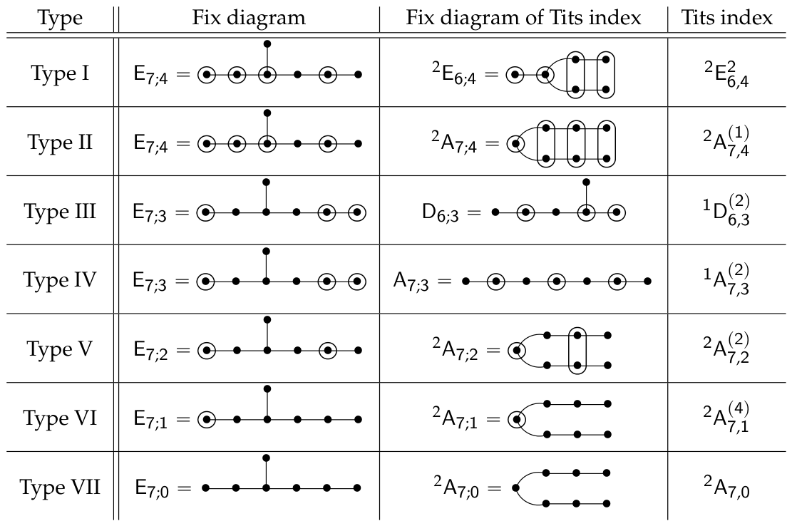
Figure 3.
The fix diagrams and .

Disclaimer/Publisher’s Note: The statements, opinions and data contained in all publications are solely those of the individual author(s) and contributor(s) and not of MDPI and/or the editor(s). MDPI and/or the editor(s) disclaim responsibility for any injury to people or property resulting from any ideas, methods, instructions or products referred to in the content. |
© 2026 by the authors. Licensee MDPI, Basel, Switzerland. This article is an open access article distributed under the terms and conditions of the Creative Commons Attribution (CC BY) license (http://creativecommons.org/licenses/by/4.0/).
Copyright: This open access article is published under a Creative Commons CC BY 4.0 license, which permit the free download, distribution, and reuse, provided that the author and preprint are cited in any reuse.