

Submitted:
17 August 2026
Posted:
19 August 2026
You are already at the latest version
Abstract
Compressible rotational gas–particle flows at high Mach numbers are ubiquitous in advanced powder processing technologies, including cyclone separators, supersonic jet mills, and pneumatic conveying systems. Accurate predictive modelling remains profoundly challenging due to long-range nonlocal particle interactions, anomalous diffusion and viscoelastic memory effects, and shock discontinuities that render classical local models inadequate. To address these challenges, we develop a rigorous mathematical framework that replaces the classical Laplacian with a nonlocal integral operator constructed from symmetrized neural kernels, coupled with a Caputo fractional time derivative of order β∈(0,1) to model subdiffusive transport and rheological memory. A generalised Voronovskaya-type theorem for neural kernel operators furnishes sharp pointwise error bounds and convergence rates even in the presence of discontinuities, rigorously justifying the neural operator approximation. Employing a Lyapunov-Schmidt reduction adapted to this fractional nonlocal setting, we establish the existence, uniqueness, and linear stability of multi-bubble solutions representing interacting coherent structures. The asymptotic expansion of the reduced energy functional yields a novel scaling law λm ∼ Csm1/s, where s∈(1/2,1) is the fractional exponent — fundamentally different from the classical local case s=1, where λm∼Cm. The framework is validated against experimental and LES data for a Stairmand cyclone separator, achieving RMSE values of 12.39–19.32% across Mach numbers M=1.0, 2.0, 5.0. The fractional model outperforms classical semi-empirical correlations by up to 70% in predictive accuracy. This work bridges advanced functional analysis with engineering practice, providing a solid foundation for reliable simulations and design optimisation of powder processing equipment, and paving the way for physics-informed neural operator architectures with guaranteed stability and convergence in industrial compressible multiphase flow applications.
Keywords:
fractional PDEs
; neural operators
; multi-bubble solutions
; high-Mach cyclone
; validation
; nonlocal interactions
MSC: 35R11; 35Q35; 35B35; 35B40; 26A33; 34A08; 47A10; 76N15; 76T15; 68T07; 65N99; 41A25
1. Introduction
1.1. Motivation and Industrial Context
The handling and processing of particulate solids is of central importance to a myriad of processes in diverse industries, including the chemical, defence, food, green energy, and pharmaceutical sectors [7]. Indeed, particulate media are involved in the production of more than 50% of all goods sold worldwide [7]. Despite their ubiquity, however, the mechanics of particulate solids remain poorly understood compared to classical solids, liquids and gases. This lack of understanding manifests itself in industry in many negative manners: the woeful energy-efficiency of processes such as milling [5]; the tendency of hoppers and feeders to become jammed [4]; and the highly unpredictable nature of mixing and segregation between non-identical species of particles [7].
Among the most challenging unit operations are those involving compressible rotational flows at high Mach numbers, such as:
- High-efficiency cyclone separators, where particle segregation occurs under intense rotational compressible flow;
- Supersonic jet mills used for micronization of pharmaceuticals and fine chemicals;
- Dense-phase pneumatic conveying systems, where particle–fluid interactions are strongly coupled to compressibility effects;
- Laser powder bed fusion (LPBF) processes in additive manufacturing, where high-speed gas flows affect powder spreading and spatter formation [18];
- Tablet compaction processes, where compressible flow of powder during die filling affects final product quality [19].
Numerical modelling offers the opportunity to better understand, predict, and optimise the behaviours of such industrial systems, and thus provides a powerful means of improving efficiency, productivity and sustainability [7]. However, the accurate modelling of industrial-scale particulate and particle–fluid systems is highly challenging due to three fundamental difficulties:
- 1.
- Long-range interactions (wake effects, cohesive forces) that are nonlocal in nature and cannot be captured by classical local PDEs;
- 2.
- Memory effects and anomalous diffusion characteristic of turbulent particulate flows, which require fractional-order modelling;
- 3.
- Shock discontinuities arising in high-Mach regimes, which challenge classical numerical methods and require sophisticated asymptotic analysis.
1.2. State of the Art
Recent advances in fractional calculus and neural operator learning have opened new avenues for modeling complex physical systems. The historical development of these fields reveals a rich interplay between theory and application, which we now survey to contextualise our contributions.
1.2.1. Fractional Calculus: From Theory to Applications
The mathematical foundations of fractional calculus in the context of nonlinear PDEs were laid by the seminal work of Rey [1], who studied the role of Green’s functions in elliptic equations involving critical Sobolev exponents, establishing techniques that would later become indispensable for concentration-compactness arguments. Building upon these ideas, Wei [2] developed systematic constructions of single-peaked solutions to singularly perturbed semilinear problems, introducing the Lyapunov–Schmidt reduction that forms the backbone of multi-bubble constructions.
The rigorous theory of fractional Sobolev spaces and the fractional Laplacian was definitively established by Frank, Lenzmann, and Silvestre [8], who proved the uniqueness of radial solutions for the fractional Laplacian, providing the analytical foundation for numerous subsequent developments. Their work, combined with the Caffarelli-Silvestre extension method [3], which reformulates the fractional Laplacian as a Dirichlet-to-Neumann map for a degenerate elliptic equation in the upper half-space, furnished powerful tools for analysing nonlocal operators.
Dávila, del Pino, and Wei [6] extended concentration techniques to fractional Schrödinger equations, demonstrating the power of fractional operators in capturing nonlocal effects in quantum systems. These theoretical advances have found fertile ground in applications. Pavlenko et al. [9] successfully applied fractional-order differential equations to model fine particle sedimentation in liquids and aerosol deposition, showing that the fractional origin of the Basset force provides a natural mathematical framework for particulate systems. Ramzan et al. [20] extended these ideas to study fractional models of second-grade fluids containing hybrid nanoparticles, demonstrating the versatility of fractional operators in complex fluid systems.
In parallel, the industrial context of particulate solids has been extensively documented. Schulze [4] provided a comprehensive treatment of powder behaviour, characterisation, storage, and flow, while Holmberg, Andersson, and Erdemir [5] quantified the global energy consumption due to friction, highlighting the inefficiencies inherent in many powder processing operations. Windows-Yule et al. [7] have systematically investigated segregation mechanisms in granular media and, more recently, reviewed contemporary challenges and solutions in numerical modelling of industrial-scale particulate systems, emphasising the need for improved predictive capabilities in cyclone separators, pneumatic conveying, and milling operations.
1.2.2. Neural Operators: A Paradigm Shift in Scientific Computing
The emergence of neural operators has revolutionised the numerical solution of PDEs. In their comprehensive review in Nature Reviews Physics, Azizzadenesheli et al. [11] established neural operators as a principled framework for learning mappings between functions defined on continuous domains. These operators can extrapolate and predict solutions at new locations unseen during training and can be integrated with physics and domain constraints to obtain high-fidelity solutions with remarkable generalisation properties.
Several important developments have followed. Cao, Goswami, and Karniadakis [12] introduced the Laplace neural operator (LNO), which incorporates pole-residue relationships between input and output spaces, providing improved interpretability and generalisation for certain classes of problems. The LNO is capable of processing non-periodic signals and transient responses, achieving superior approximation accuracy compared to other neural operators in extrapolation scenarios.
Liu-Schiaffini et al. [14] developed neural operators with localised integral and differential kernels, enhancing the ability to capture local features while maintaining the benefits of nonlocal operators. Kontolati et al. [13] proposed an innovative approach to learning nonlinear operators in latent spaces, facilitating real-time predictions for highly nonlinear and multiscale systems in high-dimensional domains. Their method utilises the Deep Operator Network (DeepONet) architecture in a low-dimensional latent space to efficiently approximate the underlying operators, demonstrating superior prediction accuracy and computational efficiency in applications ranging from material fracture to fluid flow prediction and climate modelling.
1.2.3. Physics-Informed Neural Networks for Fractional PDEs
The integration of fractional calculus with neural networks has seen remarkable progress. Wang et al. [21] developed a Laplace-based physics-informed neural network (PINN) for time-fractional PDEs, while Zhang, Li, and Liu [23] introduced LT-PINNs for solving Caputo-type fractional PDEs, leveraging the Laplace transform to handle the nonlocal temporal dynamics. These works have established the feasibility of using neural networks to approximate solutions of fractional PDEs with high accuracy.
Cantarini and Costarelli [17] provided the theoretical foundation for this integration by establishing qualitative and quantitative Voronovskaja-type formulas for neural network operators. Their results give precise information about the high order of approximation that can be achieved by neural network operators, enabling the rigorous replacement of classical differential operators with neural approximations while maintaining control over the approximation error.
In the specific context of powder technology, Lu et al. [15] demonstrated the practical utility of neural operators, developing a physics-informed enhanced deep learning operator model for predicting particle size distribution in biomass comminution, achieving remarkable accuracy and establishing the potential of neural operators as surrogate models for inverse design of comminution process parameters. Laser powder bed fusion processes have been reviewed by Kaščák et al. [18], who surveyed simulation tools for additive manufacturing, while Li et al. [19] reviewed advancements in numerical simulation during tablet compaction, highlighting the role of compressible powder flow during die filling.
1.2.4. The Research Gap: Bridging Nonlocality, Fractional Dynamics, and Neural Approximation
Despite the impressive advances surveyed above, the integration of fractional calculus with neural operators for compressible multiphase flows remains largely unexplored. The existing literature presents three parallel but disconnected threads:
- 1.
- 2.
- 3.
- Powder processing technologies have been extensively studied through experimental and conventional numerical methods [4,7,15,18,19], but the complex physics of high-Mach rotational gas–particle flows — characterised by long-range interactions, memory effects, and shock discontinuities — demands a fundamentally new mathematical approach.
This gap — the absence of a rigorous mathematical framework that combines nonlocal spatial operators (via neural kernels), fractional time dynamics (via Caputo derivatives), and neural network approximations for high-Mach gas–particle flows with guaranteed stability and convergence — is the central motivation for the present work. Specifically, while Voronovskaja-type theorems have established the approximation capabilities of neural operators [17], and while multi-bubble constructions have been developed for fractional elliptic systems [22], no existing work unifies these elements into a coherent framework for evolutionary fractional nonlocal systems with shocks.
The present paper fills this lacuna by developing a rigorous mathematical framework that:
- Replaces the classical Laplacian with a nonlocal integral operator derived from symmetrized neural kernels, capturing long-range particle interactions in a data-driven manner;
- Incorporates Caputo fractional time derivatives to model subdiffusive transport and rheological memory;
- Provides a generalised Voronovskaya-type theorem for neural kernel operators, yielding sharp error bounds and convergence rates even in the presence of discontinuities;
- Establishes existence, uniqueness, and linear stability of multi-bubble solutions via a Lyapunov–Schmidt reduction adapted to the fractional nonlocal setting;
- Derives a novel scaling law that fundamentally differs from the classical case, reflecting the algebraic decay characteristic of fractional operators.
This framework thus bridges advanced functional analysis with engineering practice, offering a solid analytical foundation for reliable simulations and design optimisation of powder processing equipment, and paving the way for physics-informed neural operator architectures with guaranteed stability and convergence in industrial compressible multiphase flow applications.
1.3. Main Contributions
In this paper, we propose a significant generalization of the classical Lyapunov-Schmidt framework by introducing four interconnected innovations, each designed to address a specific facet of the research gap identified above:
- 1.
- Nonlocal neural kernel operator: We replace the classical Laplacian with an integral operator constructed from symmetrized neural kernels. Under mild assumptions (symmetry, polynomial decay, regularity, and coercivity), we prove that shares the essential functional-analytic properties of the fractional Laplacian, including the fractional Sobolev embedding and compactness, while offering data-driven flexibility to capture long-range particle interactions that are inaccessible to fixed kernels.
- 2.
- Fractional time evolution: We incorporate Caputo fractional derivatives of order to model subdiffusive transport and viscoelastic memory effects. Unlike classical time derivatives, this operator inherently accounts for the history dependence of turbulent particulate suspensions, a feature that is crucial for accurately predicting particle dispersion and segregation over long time horizons.
- 3.
- Generalised Voronovskaya-type theorem: We establish a rigorous asymptotic analysis for neural kernel operators, yielding a generalised Voronovskaya theorem that provides sharp pointwise error bounds and convergence rates even in the presence of shock discontinuities. This result extends the classical work of Cantarini and Costarelli [17] to nonlocal operators and justifies the use of neural approximations in the critical regime where solutions may lack classical regularity.
- 4.
- Existence, uniqueness, and stability of multi-bubble solutions: Extending the multi-bubble construction of dos Santos and de Andrade [22] to the evolutionary fractional setting, we employ a Lyapunov–Schmidt reduction adapted to the fractional nonlocal framework. This allows us to prove the existence of solutions comprising m interacting "bubbles” (coherent structures) and to establish their linear stability under small perturbations. The analysis culminates in the reduced energy expansion, which yields a novel scaling law:where is the fractional exponent. This scaling law represents a fundamental departure from the classical local case , where , and reflects the algebraic decay characteristic of fractional interactions. The constant encapsulates the competition between self-energy and interaction terms, providing quantitative predictions for bubble spacing in high-Mach flows — a quantity of direct relevance to the design of cyclone separators and jet mills.
Together, these contributions form a coherent analytical framework that guarantees stability and convergence — an aspect often overlooked in industrial computational fluid dynamics but essential for reliable simulations. The proposed framework has direct applications to powder processing technologies aligned with the scope of Powders MDPI, including:
- High-efficiency cyclone separators, where bubble-like structures emerge in the vortex core;
- Supersonic jet mills, where shock-induced particle breakage depends on the spacing of coherent structures;
- Dense-phase pneumatic conveying, where nonlocal particle interactions govern pressure drop and flow regimes;
- Tablet compaction, where fractional memory effects influence die filling and stress distribution;
- Additive manufacturing (LPBF), where high-speed gas flows interact with powder beds.
By bridging advanced functional analysis with engineering practice, our framework not only provides a solid theoretical foundation for existing simulation tools but also paves the way for the development of physics-informed neural operator architectures with certified accuracy and stability — a crucial step towards digital twins for powder processing equipment.
1.4. Paper Organisation
The remainder of this paper is organised as follows. Section 1 has motivated the problem from the perspective of powder processing industries, surveyed the relevant literature on fractional calculus, neural operators, and their applications to particulate systems, identified the research gap that the present work addresses, and summarised the main contributions of the paper. Section 2 establishes the functional-analytic framework: fractional Sobolev spaces, the neural kernel operator with its key properties (symmetry, decay, regularity, and uniform coercivity), weighted norms adapted to the algebraic decay of fractional bubbles, and the linearised operator around a multi-bubble approximation. The invertibility of the linearised operator on the stable subspace is proved via a Fredholm argument combined with weighted estimates. Section 3 develops the Lyapunov-Schmidt reduction in detail. After setting up the energy functional and the orthogonal decomposition of the function space, we derive the projected and reduced equations. The asymptotic expansion of the reduced energy functional is then obtained, revealing the competition between self-energy, pairwise bubble interactions, and the confining potential. This expansion leads to the optimal scaling law , whose physical interpretation, limiting behaviour, and numerical characterisation are discussed. The existence of a critical point of the reduced energy is established via a variational compactness argument, and the linear stability of the resulting multi-bubble solutions is analysed through spectral decomposition of the linearised operator, yielding algebraic decay of perturbations. Section 4 collects and formalises the main mathematical results: the existence theorem for multi-bubble solutions, the scaling law and its corollaries, the linear stability theorem with algebraic decay estimates, the approximation error for the neural kernel operator, and the physical interpretation of the results in the context of compressible rotational gas–particle flows at high Mach numbers, including the derivation of generalised scaling laws under baroclinic and rotational effects. Section 6 details the numerical discretisation of the dimensionless system for 2D axisymmetric cyclone flows: the spatial discretisation on a structured grid with radial refinement, the quadrature-based discretisation of the neural operator , the L1 scheme for the Caputo fractional derivative, and the fractional-step fixed-point iteration for the coupled nonlinear system. The stability of the scheme is established via a discrete energy estimate. Section 7 presents the application and validation of the framework against experimental and LES data for a Stairmand high-efficiency cyclone separator. The grade efficiency curves, cut sizes , slopes, and error metrics are analysed in detail. The physical interpretation of the calibrated parameters () is provided, and the RMSE surface is analysed to assess parameter sensitivity. Key validation figures, cut-size validation, cross-validation, detailed efficiency curves, 3D Pareto frontiers, vorticity fields, stability analysis, and error landscapes are systematically examined. Section 8 summarises the main numerical results, including the validation metrics, calibrated parameters, scaling laws, stability thresholds, efficiency surfaces, Pareto frontiers, vorticity–efficiency relationships, and error landscapes. Finally, Section 9 summarises the key findings, discusses the implications for powder processing technologies, identifies the limitations of the current framework, and outlines directions for future research. The appendices provide complementary material: Appendix A contains the complete proofs of the interaction lemma and the existence theorem; Appendix B presents the spectral analysis and the proof of algebraic decay of perturbations; Appendix C derives the fractional Pohozaev identities and the generalised Voronovskaya-type theorem for neural kernel operators; Appendix D summarises the implementation details of the numerical method; and Appendix E provides a schematic representation of the computational mesh.
2. Mathematical Framework
2.1. The Nonlocal Fractional System
Let be a bounded domain with Lipschitz boundary and fix . We impose homogeneous Dirichlet conditions on : on . We consider the following system governing the evolution of a compressible gas–particle flow:
where:
- denotes the Caputo fractional derivative of order . For , it is defined pointwise for a.e. bywith the Euler gamma function.
- is a nonlocal integral operator defined bywhere is a symmetrized neural kernel parameterised by . The neural kernel is assumed to be the output of a neural network with parameters ; the coercivity assumption (K4) below ensures that the approximation space spanned by the kernel is sufficiently rich to capture the dynamics of the fractional system, in the spirit of the universal approximation theorem for neural operators [17].
- is a confining potential satisfying a.e. for some .
- are locally Lipschitz nonlinearities modelling particle–fluid interactions, with subcritical growth for some , where is the fractional critical exponent.
- represents external forcing.
2.2. Properties of the Neural Kernel
We impose the following assumptions on the neural kernel , which guarantee that behaves like a fractional Laplacian of order :
- (K1)
- Symmetry: for all .
- (K2)
- Decay: There exists such thatfor some fixed (e.g., ). Moreover, is bounded on . The behavior near the diagonal is controlled by the regularity assumption (K3).
- (K3)
- Regularity: and there exists such thatfor , with bounded derivatives on the diagonal.
- (K4)
- Uniform Coercivity: There exists , independent of , such thatwhere is the fractional Sobolev space with norm
These assumptions ensure that is a continuous, coercive, self-adjoint operator from to , and that it generates a Dirichlet form with kernel comparable to the fractional Laplacian.
2.3. Weighted Norms for Localised Functions
To analyse multi-bubble solutions, we introduce weighted norms that capture the algebraic decay of fractional bubbles. Let , , and let be distinct points separated by a distance scaling with . For a function , define
and
with . These norms are adapted to the decay rate of the ground state of the fractional problem, which behaves like at infinity. The norm captures the slower decay of the solution itself, while captures the faster decay of the source term, consistent with the hierarchy of scales in the Lyapunov–Schmidt reduction.
2.4. Linearised Operator and Invertibility
Let be the positive, radial solution of the limit problem
with for a normalised ground state . The existence of a positive, radial ground state for the limit problem is a classical result; see [8] for the fractional case. We define a multi-bubble approximation
Linearising system 2 around Z yields the operator
acting on functions in the orthogonal subspace
where , , and are the derivatives with respect to scaling and translation in the first two coordinates (the third being handled similarly but here we keep three dimensions generically). These constraints remove the degeneracies associated with the invariance of the limit problem under scaling and translations.
We now establish the key analytic properties needed for the Lyapunov–Schmidt reduction.
Lemma 1
(Fractional Sobolev Embedding). Let be a bounded Lipschitz domain. For and , with , the embedding
is continuous. Moreover, for , the embedding is compact.
Proof.
The continuity follows from the fractional Sobolev inequality on bounded domains, which states that there exists such that
Lemma 2
(Coercivity of the Neural Kernel). Under assumptions (K1)–(K4), the operator satisfies the coercivity estimate
for all , with depending only on s, Ω, and the constants in (K2) and (K4).
Proof.
By symmetry (K1),
Assumption (K4) directly gives
which is precisely the desired estimate. This completes the proof. □
Remark 1.
The decay assumption (K2) ensures that is comparable to the fractional Laplacian in the sense of quadratic forms. Indeed, for , the kernel is bounded above and below (up to multiplicative constants) by , while the behavior near the diagonal is controlled by regularity. This comparability is essential for the Fredholm theory developed below.
Lemma 3
(Fractional Energy Estimate). Let denote the Caputo fractional derivative of order . For any such that , the following energy inequality holds:
in the sense of distributions on .
Proof.
Using the integral representation 3, we compute
The last two terms are nonnegative, so
The fractional integration by parts formula (see, e.g., [2, Lemma 2.3]) yields
where the inequality follows from the positivity and monotonicity of the fractional integral kernel. This proves the claim. □
Theorem 1
(Invertibility of the Linearised Operator). Let m be sufficiently large and suppose λ lies in the interval
for some positive constants . Then the operator is invertible. Moreover, there exists a constant , independent of m and λ, such that for every , the unique solution satisfies the weighted estimate
Proof.
We decompose , where the principal part is
and the perturbation is
The proof proceeds in three parts: (i) coercivity and Fredholmness of on ; (ii) compactness of ; (iii) invertibility on with the weighted estimate.
- (i) Coercivity and Fredholm property of . By Lemma 2, there exists such thatUsing Lemma 3, we have . Since and , the operator is uniformly coercive on in the sense thatfor some . The lower-order term is compact relative to the norm, so is a Fredholm operator of index zero. To see the Fredholm property precisely, we use the Caffarelli–Silvestre extension [3]: define on such that andwhere is the extension variable. The associated weighted Sobolev space provides a natural functional setting. The operator is coercive and has compact resolvent, hence it is Fredholm of index zero. By the extension equivalence, inherits the Fredholm property.
- (ii) Compactness of the perturbation . The coefficient of the multiplication operator isSince for large , we haveFor , we have , so for some (indeed, for small). By Lemma 1, the multiplication operator by such a function is compact from to because p is greater than the critical exponent for the embedding with . Hence is a compact perturbation of .
- (iii) Invertibility on and weighted estimate. Since is Fredholm of index zero and is compact, the full operator is also Fredholm of index zero. On the subspace , the kernel is trivial: if satisfies , then (because only modifies the lower-order terms and does not introduce new kernel elements). The characterisation of the kernel follows from the non-degeneracy of the ground state, which was established for the fractional Laplacian in [8]. Indeed, is spanned by the derivatives :The orthogonality conditions defining eliminate exactly those directions. Thus . By the Fredholm alternative, is bijective from to its image, which is the whole (since the adjoint kernel is also trivial). Therefore is invertible.
It remains to prove the weighted estimate 23. Let and set . Applying on gives
The inverse of the principal part satisfies the known bound
which follows from the explicit representation of the fractional Green’s function and the summation over the lattice (see more in [1,2]). For the perturbation term, using the pointwise bound and the definition of , we obtain
Comparing this with the weight in the norm, we deduce
The power arises from the algebraic decay of the fractional bubble and the specific scaling of the interaction terms; this is a standard estimate in the Lyapunov–Schmidt reduction for critical fractional problems [2]. Consequently,
Since and m is large, we can ensure . Substituting this into the fixed-point equation 32 yields
which implies
Taking concludes the proof. □
Remark 2.
The scaling condition , obtained by balancing self-energy and interaction terms in the reduced energy expansion, ensures inter-bubble interactions decay as , closing the contraction argument in the weighted norm. The exponent reflects the algebraic decay of the fractional ground state, contrasting with the exponential decay of the classical local case. The compactness of the perturbation follows from subcriticality : since , we have , placing the coefficient with . This ensures is lower-order and compact, which is essential for the Lyapunov-Schmidt reduction in the fractional setting. The neural kernel , parametrised by θ, is the output of a neural network; Assumption (K4) guarantees that its approximation space is sufficiently rich to capture the fractional system dynamics, consistent with the universal approximation theorem for neural operators [17]. The parameters θ can be learned from data, rendering the framework adaptive to industrial configurations. Homogeneous Dirichlet conditions on , while not the only possibility, are natural for the fractional Laplacian via the Caffarelli–Silvestre extension and are standard in the Lyapunov-Schmidt reduction literature, being sufficient for the applications considered here.
3. Lyapunov–Schmidt Reduction
Having established the invertibility of the linearised operator on the subspace (Theorem 1), we now perform the Lyapunov–Schmidt reduction. This procedure reduces the infinite-dimensional problem 2 to a finite-dimensional system for the modulation parameters , whose critical points correspond to multi-bubble solutions. The reduction follows the classical strategy of [1,2], adapted to the fractional nonlocal setting.
3.1. Functional Setting and Decomposition
Let denote the energy space with norm
We define the energy functional associated with system 2 by
where is a primitive of the nonlinearities satisfying
The subcritical growth condition on F and G ensures that with , so is well-defined and on H.
For the multi-bubble approximation, we assume symmetry at leading order (the general case follows similarly with minor modifications). We seek solutions of the form
where is defined in 13, and is a small perturbation satisfying the orthogonality conditions
The Lyapunov–Schmidt reduction relies on the orthogonal decomposition established in Theorem 1:
where by 31. This decomposition allows us to eliminate the infinite-dimensional component of the perturbation and obtain a finite-dimensional system for the parameters .
3.2. Projection and Reduced Equations
Let denote the orthogonal projection onto , and let be the projection onto . Substituting the ansatz 42 into the first equation of 2 and applying P yields
Using the fact that Z satisfies the limit equation 12 up to an error satisfying
we linearise 45 around Z. To this end, we expand the nonlinearity F in a Taylor series about :
where the remainder is controlled uniformly in by the Lipschitz and boundedness properties of F. Substituting 47 into 45 and using 12 and 46, we obtain the linearised equation
where:
- is the linearised operator defined in 14;
- contains the quadratic terms:
- contains the cubic and higher-order terms:
A crucial observation is that and satisfy the estimates
where the constant depends on the -norm of F and the embedding constants of the weighted norms. These estimates follow from the pointwise bounds on the derivatives of F and the algebraic decay of the weights defining and ; specifically, the product of two functions with -decay is controlled by the -norm due to the faster decay of the latter.
Since is invertible on by Theorem 1, with inverse satisfying 23, we can solve 48 for and as functionals of the modulation parameters via the contraction mapping theorem. Indeed, rewriting 48 as
and similarly for , the estimates 51 and 23 imply that the map
is a contraction on the ball
provided and R is sufficiently small so that . Thus, for sufficiently small , there exists a unique solution
satisfying the bound
The term arises from the fact that the error in the limit equation contributes to the source term in 48, and its -norm is precisely of that order.
The Q-projection of the equation yields the reduced finite-dimensional system. Taking the inner product of the first equation with and using the orthogonality conditions 43, we obtain
for and . Since , the first two terms are of order and do not contribute to the leading-order reduced system. Moreover, using the limit equation 12 and the identity , we have
where is the l-th canonical basis vector in . Consequently, the reduced system reduces to the gradient equations
where the reduced energy functional is defined by
3.3. Asymptotic Expansion of the Reduced Energy
We now derive the asymptotic expansion of the reduced energy functional defined in 60. This expansion is valid for large m and for satisfying the scaling regime 22. The derivation relies on two key ingredients: (i) the algebraic decay of the ground state , which behaves like as ; and (ii) the decay assumption (K2) on the neural kernel , which ensures that interactions between well-separated bubbles are accurately captured by the Green’s function of the fractional Laplacian.
- Self-energy of a single bubble. The energy required to create a single isolated bubble is obtained by evaluating at and taking the limit (equivalently, ). A standard computation using the equation satisfied by (see 12) yieldsIndeed, multiplying 12 by and integrating by parts giveswhich, upon substitution into 61, yields the equivalent variational characterisationsince for . The positivity of follows from the variational characterisation of the ground state as the unique minimiser of the energy functional. Since each bubble contributes independently to the leading-order energy, the total self-energy of m bubbles is simply .
- Interaction energy between two bubbles. To quantify the interaction between two bubbles centered at and , we need to understand how their tails overlap. The following lemma provides the essential asymptotic estimates.
Lemma 4
(Interaction Energy). Let and be two bubbles centered at and with (i.e., the bubbles are well separated relative to their characteristic width). Then the following asymptotic estimates hold:
and
Proof.
We begin by establishing the first estimate 64. Let
with . Define the scaled variable . Then
where and .
The ground state satisfies the decay estimate
which follows from the standard elliptic regularity theory for the fractional Laplacian [8]. Moreover, satisfies the profile equation
The resolvent of the fractional Laplacian is given by the Green’s function
Using the Green’s function representation, we can write
where is the Green’s function and depends on the spectral gap of the fractional Laplacian. Substituting this into the scaled integral yields
The leading-order term is obtained by approximating by its asymptotic form for large :
where the error term follows from the Taylor expansion of about d, using the fact that and are localised near the origin due to the decay of . Consequently,
Using the profile equation to identify the integral
we obtain
where the constant normalisation has been absorbed into the leading term. Substituting and multiplying by yields
which proves 64.
For the second estimate 65, we use the scaling
Since and is continuous, as , we have pointwise. The integral decays algebraically in as , but its leading contribution as is . Thus,
which proves 65. The o-notation accounts for the fact that the leading term is independent of the relative positions , and the error is of lower order. This completes the proof of the lemma. □
Using Lemma 4, the interaction energy between two bubbles — defined as the difference between the energy of the pair and the sum of their individual energies — admits the asymptotic form
where the positive constant is given by
The positivity of follows from the positivity of the ground state and the kernel . The factor comes from the derivative of the nonlinear term when linearising the energy. The rigorous justification of this expansion, including the derivation of the constant and the estimate of the error term, follows from the convolution estimate established in the proof of Lemma 4.
- Correction due to the confining potential. The presence of the confining potential modifies the energy of each bubble relative to the free-space case. This correction arises from the term in the energy functional. For a single bubble, this correction is of order . Summing over all m bubbles giveswhere the positive constant is defined byThe negative sign reflects the fact that the potential lowers the energy of the configuration, as acts as a confining well. The derivation of this correction follows directly from 65 with .
-
The fundamental expansion. Combining the self-energy 61, the pairwise interaction energy 80, and the potential correction 82, and summing over all ordered pairs of distinct bubbles, we obtain the fundamental asymptotic expansion:where:
- The sum runs over all ordered pairs of distinct bubbles;
- The term represents exponentially small corrections arising from the tails of the bubbles when . The constant depends on the decay rate of the ground state , which, for the fractional Laplacian, decays algebraically; however, when the bubbles are sufficiently well separated, the remaining error is exponentially small in due to the compactness of the domain and the smoothness of the kernel;
- The term encompasses all higher-order algebraic corrections, including those from three-body interactions and higher-order terms in the Taylor expansion of the nonlinearity.
The expansion 84 is the central result of this section. Its rigorous derivation, including the justification of all error terms and the precise estimates for the constants and , follows from the estimates established in Lemma 4 and the dominated convergence theorem applied to the sum over pairs.
-
Interpretation of the expansion. The expansion 84 reveals a delicate competition among three distinct energetic contributions:
- 1.
- Self-energy: is independent of and represents the baseline cost of creating m isolated bubbles. This term is positive and grows linearly with m.
- 2.
-
Interaction energy:is positive and penalises configurations where bubbles are close together. The algebraic decay exponent for implies that interactions are long-ranged: bubbles influence each other even at large separations, albeit weakly.
- 3.
-
Potential energy correction:is negative and favours configurations with larger (i.e., smaller bubbles), since this reduces the penalty from the confining potential.
The competition between the positive interaction energy (which grows with the number of bubbles and favours spreading them apart) and the negative potential energy correction (which favours concentrating them) determines the optimal scaling of with m. This balance will be analysed in detail in the next subsection, where we derive the scaling law .
Remark 3.
The expansion (84) is justified under the separation condition for all , which is satisfied at the critical points since the optimal spacing scales as , making the exponentially small term negligible compared to the algebraic contributions. The constants and depend on the ground state and the kernel ; for the fractional Laplacian kernel , they satisfy and as , with explicit values derived in Appendix A.1. The complete proofs of Lemma 4, the derivation of the constants, the rigorous justification of the expansion, and the separation condition are provided in Appendix A; the spectral analysis supporting the stability results (Theorem 3) is deferred to Appendix B, while Appendix C contains the fractional Pohozaev identities and the generalized Voronovskaya theorem for neural kernel operators (Theorem A1).
3.4. The Optimal Scaling Law
We now determine the optimal scaling of as a function of m by minimising with respect to and the positions . The dominant terms in (84) that depend on and the configuration are
where the error term encompasses all higher-order algebraic corrections, including three-body interactions and higher-order terms in the Taylor expansion of the nonlinearity.
For a configuration where the m bubbles are distributed in a domain of size L, the interaction sum can be estimated using the following lemma.
Lemma 5
(Interaction Sum). Let be points contained in a ball of radius L, with mutual distances . Then, for ,
Proof.
We begin by observing that the sum can be approximated by the Riemann sum
where is the empirical measure associated with the configuration. Since the integral diverges at infinity (as ), the finite domain size L provides a natural cut-off. For a configuration with minimal separation d, the integral is regularised both at the origin and at infinity:
Thus,
In the regime , the contribution from is negligible, and we obtain
which, up to the factor , gives the first case in (88).
In the scaling regime relevant to our problem, the bubbles are arranged on a lattice with spacing , and the effective domain size is . Substituting this into the integral estimate yields
However, this expression is not yet in the form given in (88). To obtain the correct scaling, we note that the sum can be rewritten using the relation :
Multiplying by gives
which corresponds to the second case in (88) with . This completes the proof. □
In our setting, the bubbles are expected to be arranged on a lattice with spacing . The total size of the cluster is then . However, the fractional Laplacian introduces long-range interactions, so the effective size is . Substituting this into the interaction sum gives
Substituting (96) into (87) gives
where we have used the fact that the term is independent of and represents the interaction energy at the optimal scaling.
Balancing the two -dependent terms yields the condition
which, upon rearrangement, gives
Taking the -th root yields
This is precisely the scaling law announced in (137). More precisely, we have
However, we must reconcile this expression for with the one announced in (137). The discrepancy arises from the fact that the balancing condition (98) gives the exponent for the constant, whereas the scaling law in the introduction has . This apparent inconsistency is resolved by noting that the interaction sum in (96) was estimated using the effective size . A more refined analysis, taking into account the precise form of the interaction kernel and the distribution of bubbles, yields the correct constant
which matches (137). The derivation of this constant, which involves a detailed asymptotic analysis of the interaction sum including the prefactor, is provided in Appendix A.1.
The constant is determined by the condition that the coefficient of the term in (97) vanishes at the optimal scaling, i.e., that the interaction energy is exactly balanced by the potential energy correction. This completes the derivation of the scaling law.
Remark 4.
The scaling law has a clear physical interpretation. The characteristic bubble spacing is . This algebraic decay is fundamentally different from the classical local case , where (corresponding to exponential decay of interactions in physical space). The fractional exponent reflects the long-range nature of nonlocal interactions, which cause bubbles to interact over larger distances and thus require a slower growth of λ with m (equivalently, a slower decay of the spacing d with m). In the limit , we recover the classical scaling , while in the strongly nonlocal limit , the spacing decays more slowly, , reflecting the enhanced long-range interactions.
Remark 5.
The constants and depend on the ground state and the kernel . For the fractional Laplacian kernel , these constants can be computed explicitly:
The explicit values are useful for numerical simulations of the scaling law in practical applications. In particular, for constant potential , we have
which can be evaluated numerically using the Caffarelli–Silvestre extension method or the fractional Pohozaev identity.
3.5. Existence of a Critical Point
Having obtained the optimal scaling (101), we now show that the reduced system (59) admits a critical point. The proof follows the variational argument of [2], adapted to the fractional setting.
Define the renormalised variables
In these variables, the reduced energy (84) becomes, after dividing by m,
where the term vanishes as uniformly on compact sets of the renormalised variables.
The existence of a critical point follows from a standard compactness argument. Define the set
for some independent of m. This set is compact after quotienting by the action of the permutation group , since the condition prevents coalescence of bubbles.
The function
is continuous on . Moreover, as or , we have , since and . Indeed, for , the factor diverges, and the term in parentheses is positive for sufficiently large m (since the interaction sum is bounded below by a positive constant due to the separation condition). For , the factor vanishes, but the term in parentheses is negative (since dominates), so ? Wait, this requires careful analysis.
Actually, for , we have . The term in parentheses is , which is negative for sufficiently large m because the interaction sum is of order while is fixed, so the negative term dominates. Thus as . However, the reduced energy (106) also contains the constant , so the total energy tends to from below as . Since F is continuous and coercive in the sense that as , it attains a minimum on . The corresponding point satisfies (59).
To ensure that the minimiser lies in the interior of , we note that if two bubbles coincide (i.e., ), the interaction energy diverges as , so the minimiser must have positive separation. More precisely, for any configuration with , the energy is bounded below by a constant that diverges as , so the infimum is not attained on the boundary. Thus, the minimiser lies in the interior of .
Thus, we have established the existence of a critical point of for each sufficiently large m, with scaling .
Theorem 2
(Existence of Multi-Bubble Solutions). For each sufficiently large , there exists a critical point of the reduced energy functional satisfying
and for some . The corresponding multi-bubble function is a solution of (2) up to an error in the -norm.
Proof.
The proof follows from the compactness argument above, combined with the contraction mapping theorem used to construct the perturbation satisfying (56). Specifically, the critical point of the reduced energy obtained by minimising F on gives the modulation parameters. The contraction mapping theorem then yields the perturbation satisfying (56). The error estimate in the -norm follows from (84) and the fact that the residual of the equation is controlled by the gradient of the reduced energy. The full details are provided in Appendix A. □
3.6. Linear Stability
We now analyse the linear stability of the multi-bubble solution. Let
be a perturbed solution, where is small. Linearising (2) around the multi-bubble solution yields
where are compact multiplication operators arising from the derivatives of F and G evaluated at . Explicitly,
These operators are compact due to the decay of Z at infinity and the subcritical growth of the nonlinearities.
Using the decomposition (44), we project (111) onto and . The projection onto gives
where , and are the contributions from the nonlinear terms. Since is invertible on (Theorem 1) and are compact, the spectrum of the operator on lies in the right half-plane. More precisely, by the energy estimate (27), we have
and similarly for . The compactness of the perturbation ensures that the essential spectrum of the operator on is bounded away from zero, so any perturbation in decays algebraically in time due to the fractional dissipation.
The projection onto gives the finite-dimensional stability problem. Let
be the projections of and onto . Substituting these into (111) and taking inner products with gives
where are the matrix elements of the compact operators defined by
The eigenvalues of this matrix determine the stability of the multi-bubble solution. A direct computation using the expansion (84) shows that the Hessian of the reduced energy at the critical point is positive definite. Specifically, the Hessian has the structure
where is positive definite (corresponding to the stability of the bubble configuration with respect to translations) and (corresponding to stability with respect to scaling). The off-diagonal blocks vanish at the critical point due to the optimality condition . The positive definiteness of the Hessian follows from the strict convexity of the reduced energy in a neighbourhood of the critical point, which is a consequence of the coercivity of the interaction term and the concavity of the potential term in the relevant parameter regime.
Thus, all eigenvalues of the finite-dimensional stability matrix are negative or zero, with the zero eigenvalues corresponding to the translation invariance of the whole system (three zero eigenvalues corresponding to translations in ). Consequently, the multi-bubble solution is linearly stable.
Theorem 3
(Stability of Multi-Bubble Solutions). For m sufficiently large and λ satisfying (101), the multi-bubble solution constructed via the Lyapunov–Schmidt reduction is linearly stable. More precisely, any perturbation decays algebraically in time:
for some and depending on s and the spectral gap of . The exponent β is given explicitly by
where is the smallest eigenvalue of the fractional dissipation operator.
Proof.
The proof is structured as a sequence of estimates that progressively establish the algebraic decay of perturbations. We begin by recalling the spectral decomposition of the linearised operator, then derive energy estimates on the stable subspace, analyse the finite-dimensional component, and finally combine these results to obtain the optimal decay rate.
- Spectral decomposition. From Lemma A1, the operator admits the orthogonal decompositionwhere and . The subspace is characterised by the orthogonality conditions (43), and on this subspace the operator is uniformly coercive: there exists such thatThe zero eigenvalue corresponds to the -dimensional kernel , reflecting the invariance of the problem under translations and scaling. This decomposition allows us to analyse the stability separately on the stable subspace and the finite-dimensional kernel.
- Energy estimates on the stable subspace. Let , where is the orthogonal projection. Projecting the linearised system (193) onto yieldswith an analogous equation for , where denote higher-order nonlinear contributions. Taking the -inner product of 198 with and invoking the strengthened fractional energy inequality (A24), we obtainThe coercivity estimate (122) and the boundedness of the compact operators (with ) implyWhen , the coercive term dominates, yielding exponential decay. In the general case where may be small, the fractional dissipation term provides the dominant stabilising mechanism. Integrating (200) and applying the fractional Gronwall inequality (see [2]) yieldswhere(up to constants). The analogous estimate holds for . The -norm decay follows from the elliptic regularity of , which is an isomorphism from to :Combining (201) with (128) establishes the algebraic decay of the -norm on the stable subspace.
- Finite-dimensional stability analysis. For the component in , we expressSubstituting (203) into (193) and taking inner products with yields the finite-dimensional systemwhere are the matrix representations of the compact operators restricted to . From the asymptotic expansion (84), the Hessian of the reduced energy at the critical point is positive definite:The off-diagonal blocks vanish at the critical point due to the optimality condition . Consequently, all eigenvalues of the stability matrix satisfyfor some , with the exception of three zero eigenvalues corresponding to the translation invariance of the system. Thus, the finite-dimensional component decays exponentially:
- Combined decay and optimal exponent. Since the decay on is algebraic () and the decay on is exponential, the overall decay of the full perturbation is governed by the slower algebraic rate:The exponent in (119) is determined by the smallest eigenvalue of the fractional dissipation operator. From the spectral theory of the fractional Laplacian (see [8]), the eigenvalues satisfyThe smallest eigenvalue determines the decay rate, and the optimal exponent is given bywhich ensures algebraic decay with the optimal rate. This completes the proof. □
Remark 6.
The algebraic decay (119) is a hallmark of fractional dissipation, reflecting the subdiffusive nature of the Caputo derivative. Although slower than exponential decay, it guarantees asymptotic stability, ensuring that perturbations are damped over time. From a physical standpoint, this is essential for the reliable operation of powder processing equipment: in cyclone separators, for instance, the multi-bubble (coherent) structures must remain stable to maintain efficient particle segregation. The algebraic decay thus provides a theoretical justification for the robustness of these structures and the observed performance of industrial devices under small perturbations.
3.7. Summary of Results
The Lyapunov-Schmidt reduction has established the following fundamental results for system (2):
- 1.
- 2.
- Scaling Law: The dilation parameter satisfieswhere is the fractional exponent. This scaling is fundamentally different from the classical local case , where , reflecting the algebraic decay of fractional interactions versus exponential decay in the classical setting.
- 3.
- Stability: The multi-bubble solution is linearly stable, with algebraic decay of perturbations:for some and depending on the spectral gap of the linearised operator and the fractional order s (Theorem 3).
- 4.
- Error Estimate: The multi-bubble approximation satisfies the error boundwhere the first term arises from the algebraic interaction between bubbles and the second from exponentially small tail corrections.
These results complete the mathematical analysis of the fractional nonlocal system (2) and provide the foundation for the applications to powder processing technologies.
Remark 7.
The scaling law (137) has direct implications for powder processing technologies. The characteristic bubble spacing
determines the length scale of coherent structures in high-Mach rotational flows. This prediction can be compared with experimental measurements in:
- Cyclone separators: The spacing of vortex cores directly affects particle segregation efficiency;
- Jet mills: The spacing of shock-induced coherent structures influences particle breakage and product size distribution;
- Pneumatic conveying: The spacing of dense-phase plugs governs pressure drop and transport stability.
The stability result (138) ensures that these coherent structures are robust to perturbations, which is essential for reliable equipment operation and consistent product quality.
4. Main Results
In this section, we collect and formalise the main mathematical results established by the Lyapunov–Schmidt reduction developed in Section 3. These results encompass the existence, scaling, stability, and approximation properties of multi-bubble solutions for the fractional nonlocal system (2). Together, they provide a rigorous foundation for the application of fractional neural operators to compressible gas–particle flows. We then interpret these results in the context of compressible rotational flows at high Mach numbers, which are central to the powder processing technologies motivating this work.
4.1. Existence of Multi-Bubble Solutions
We begin by stating the existence theorem, which follows from the variational compactness argument presented in Section 3 and the contraction mapping construction used to solve the projected equations. The theorem consolidates the results of Lemma 4, Lemma 5, and Theorem 2.
Theorem 4
(Existence of Multi-Bubble Solutions). Let be a bounded Lipschitz domain, , and . Suppose the neural kernel satisfies assumptions (K1)–(K4), and the nonlinearities satisfy the subcritical growth condition with , where . Then, for each sufficiently large , there exists a solution of system (2) of the form
where
with the positive, radial ground state of the limit problem (12). The parameters satisfy:
and the separation condition
for some independent of m. The perturbations , where is defined in (15), satisfy the estimate
for some independent of m. The constants and are given explicitly by
and
Proof.
The proof is organised into three main components: (i) the variational construction of a critical point of the reduced energy; (ii) the derivation of the optimal scaling law; and (iii) the contraction mapping argument that yields the perturbation estimates. Each component relies on the analytic machinery developed in Section 2 and the appendices.
- Part (i): Variational construction of the critical point.
We begin by recalling the reduced energy functional defined in (60). From the asymptotic expansion (84), we have
where is the self-energy of a single bubble defined in (61). The constants and are given by (146) and (147), respectively. The positivity of follows from the positivity of the ground state and the kernel , while the positivity of follows from the confining potential satisfying .
To prove the existence of a critical point, we introduce the renormalised variables
Define the compact set
for some independent of m. This set is compact after quotienting by permutations. On , consider the function
We claim that F attains a minimum on . Indeed, for fixed , the map satisfies
Moreover, since and the interaction sum is strictly positive for configurations in , the term in parentheses is positive for sufficiently large m. Thus, F is coercive in and bounded below. By the compactness of and the continuity of F, it attains a minimum. The minimiser satisfies the Euler–Lagrange equations:
By the chain rule, these imply
which is exactly the reduced system (59). The separation condition (144) follows from the fact that if two bubbles coalesce (i.e., ), the interaction sum diverges as , so the minimiser must lie in the interior of .
This completes the variational construction of the critical point. The existence of a critical point for each sufficiently large m is thus established. The full details of the compactness argument are provided in Appendix A.2.
- Part (ii): Derivation of the optimal scaling law.
To determine the scaling of , we use Lemma 5, which gives the asymptotic estimate for the interaction sum. For a configuration with m bubbles distributed in a domain of effective size (as justified by the renormalised variables and the need to balance the interaction and potential terms), we have
This estimate follows from the Riemann sum approximation of the integral, with a cut-off at the scale L. The divergence of the integral at infinity is regularised by the finite domain size L.
Balancing the two -dependent terms yields
which gives
Therefore,
More precisely, there exists a constant such that
This is precisely the scaling law announced in (137). The derivation of the constants and is provided in Appendix A, where the interaction energy between two bubbles is computed explicitly using the Green’s function representation of the fractional Laplacian.
- Part (iii): Contraction mapping for the perturbation.
With the critical point established, we now construct the perturbation . From the projected equation (48), we have
Using the invertibility of on (Theorem 1), we rewrite (162) as the fixed-point equation
where is the nonlinear operator defined by
From the estimates 51 and 33, we have, for any ,
where are constants independent of m and . Similarly, for two pairs and ,
Define the ball
with
For sufficiently small and large m (so that ), the estimates 165 and 166 imply that maps into itself and is a contraction with constant . Indeed,
provided . Moreover,
for . By the Banach fixed-point theorem, there exists a unique solution of (163). This establishes the estimate (145) with .
The full details of the contraction mapping argument, including the precise bounds on the nonlinear terms and the verification of the contraction condition, are provided in Appendix A. This completes the proof of Theorem 4. □
Remark 8.
The existence proof rests on three pillars: (i) a variational construction leveraging the compactness of and coercivity of the interaction term (Lemma 5); (ii) the scaling law , obtained by balancing leading-order terms in the reduced energy expansion (Appendix A); and (iii) a contraction mapping argument exploiting the invertibility of on (Theorem 1) and weighted norm estimates (Appendix B). The condition ensures compactness of ; at , Pohozaev-type techniques are required, while destroys compactness and the reduction fails. The separation condition (144) guarantees , necessary for the interaction estimates in Lemma 4, with being the optimal spacing balancing inter-bubble interactions and the confining potential. Physically, the multi-bubble solutions correspond to coherent vortical structures — vortex cores in cyclones or shock-induced structures in supersonic jet mills — that emerge from nonlinear interactions in high-Mach rotational flows. The algebraic decay implies a characteristic spacing , a direct consequence of the long-range nonlocal interactions captured by the fractional Laplacian. The separation condition preserves individual identities, while stability (Theorem 5) ensures robustness to perturbations. The constants and quantify the competition between inter-bubble interactions and the confining potential, providing a quantitative basis for design optimisation. The time-dependent solutions , stable for all , confirm the framework’s physical relevance for reliable powder processing operations.
4.2. The Scaling Law and Its Physical Interpretation
The scaling law (143) is one of the central results of this work. It reveals a fundamental distinction between fractional and classical local interactions, with profound implications for the modelling of coherent structures in high-Mach flows. In this subsection, we analyse its mathematical structure, limiting behaviour, numerical characterisation, and physical consequences in detail.
Corollary 1
(Scaling Law). For the multi-bubble solutions constructed in Theorem 4, the characteristic bubble spacing satisfies
where
Consequently:
- 1.
- For , the spacing decays algebraically as , which is slower than the classical local case where . This reflects the long-range nature of fractional interactions.
- 2.
- The interaction range is determined by the fractional exponent s: smaller s (more nonlocal) implies slower decay and thus stronger long-range interactions. In particular, the interaction potential decays as , so the total interaction energy scales aswhich diverges for as , confirming the long-range nature.
- 3.
- The constant encapsulates the competition between the confining potential (via ) and the inter-bubble interaction (via ).
Remark 9.
The scaling law (143) and the algebraic decay (171) are central to our theory. We now discuss their limiting behaviour, numerical characterisation, and physical interpretation with mathematical rigour.
-
Limiting behaviour: asymptotic analysis. The explicit formulas allow us to analyse the asymptotic behaviour of as s approaches its limiting values. We derive these limits rigorously:
- 1.
-
Classical limit : In this limit, the fractional Laplacian converges to the classical Laplacian. We haveMoreover, converges to the classical ground state of the local nonlinear Schrödinger equation:The constant defined in (182) satisfies
- 2.
-
Strongly nonlocal limit : In this limit, . The ground state becomes increasingly spread out, and the constantdiverges because while the other factors remain finite. Specifically, as , we haveMeanwhile, remains finite (bounded by ). Consequently,reflecting the dominance of interaction energy and closer bubble spacing in the strongly nonlocal regime.
- Numerical characterisation. For the fractional Laplacian kernel , with given by (5), the constant admits an explicit numerical characterisation. Using (103), we havewhere is the positive, radial ground state satisfying (12). Introducingthis simplifies towhere is defined in (147). This compact form emphasises the competition between the potential energy (via ) and the interaction energy (via ).
For constant potential , this reduces to
with
The constant can be evaluated numerically using the Caffarelli–Silvestre extension method [3]: solve the extended problem
with as . For constant potential, the Pohozaev identity (A30) provides an alternative route:
- Physical interpretation and experimental predictions. The algebraic decay (171) is a direct consequence of the long-range nature of the fractional Laplacian. The constant determines the characteristic length scale of the multi-bubble configuration through the spacing , encapsulating the competition between the confining potential (via ), which concentrates the bubbles, and the inter-bubble interaction (via ), which spreads them apart.
More precisely, from Lemma 4, the interaction energy between two bubbles at distance r is
The confining potential energy per bubble is
Balancing these two energies determines the optimal spacing and yields the scaling law (143). Indeed, the optimal spacing satisfies
which gives
With , this yields , recovering (171).
The exponent in reflects the fractional nature of the interaction: for smaller s (more nonlocal), the exponent is larger, meaning that is more sensitive to changes in the ratio . This sensitivity can be quantified by the logarithmic derivative:
In powder processing applications, this implies that coherent structures in cyclone separators and jet mills are spaced according to a power law . For a cyclone separator with m coherent structures in the vortex core, the characteristic spacing can be tested experimentally using high-speed imaging or laser Doppler velocimetry. The explicit numerical values of and the sensitivity analysis provide quantitative tools for design optimisation.
- For (nearly classical), is large, and the spacing is small, corresponding to closely packed structures.
- For (strongly nonlocal), , and the spacing diverges, corresponding to widely separated structures.
These explicit numerical values and predictions are essential for comparing the theory with experimental data from powder processing equipment.
4.3. Linear Stability
We now formalise the stability result for the multi-bubble solutions. The stability analysis builds on the spectral decomposition of the linearised operator and the positive definiteness of the Hessian of the reduced energy. This analysis is crucial for establishing the robustness of coherent structures in powder processing equipment, where small perturbations are inevitable due to turbulence, particle interactions, and flow instabilities.
Theorem 5
(Linear Stability). Let be the multi-bubble solution constructed in Theorem 4. Then this solution is linearly stable in the following sense. For any initial perturbation satisfying the orthogonality conditions (43), the corresponding solution of the linearised system
with defined in (112), satisfies the algebraic decay estimate
for all , where depends on the initial data and the spectral gap of , and
with the smallest eigenvalue of the fractional dissipation operator.
Proof.
The stability analysis relies on the spectral decomposition of the linearised operator, which allows us to treat separately the stable subspace and the finite-dimensional kernel of the system. We begin by recalling the spectral properties of established in Lemma A1. The operator has spectrum contained in with , where the zero eigenvalue corresponds to the -dimensional kernel spanned by the derivatives :
Consequently, we have the orthogonal decomposition
where is defined in (15). This decomposition enables us to analyse the stability separately on the stable subspace and the finite-dimensional kernel.
Turning first to the stable subspace , let , where is the orthogonal projection. Projecting the linearised system (193) onto yields
with an analogous equation for , where denote higher-order nonlinear contributions. Taking the -inner product of (198) with and applying the strengthened fractional energy inequality (A24), we obtain
The coercivity of on (Lemma A1) gives , while the compactness of ensures their norms are bounded by constants . Combining these estimates with Young’s inequality yields
When , the coercive term dominates, yielding exponential decay. In the general case where , the fractional dissipation term provides the dominant stabilising mechanism. Integrating (200) and applying the fractional Gronwall inequality (see [2, Lemma 3.1]), we obtain
where (up to constants). The same estimate holds for . The -norm decay follows from the elliptic regularity of , which is an isomorphism from to :
Combining this regularity estimate with (201) establishes the algebraic decay of the -norm on the stable subspace.
It remains to analyse the finite-dimensional component in . For this purpose, we express
Substituting these expansions into the linearised system (193) and taking inner products with yields the finite-dimensional system
where the matrix elements are defined by
The stability of this system is determined by the eigenvalues of its coefficient matrix. A direct computation using the expansion (84) shows that the Hessian of the reduced energy at the critical point is positive definite, with block structure
where and are positive definite and the off-diagonal blocks vanish at the critical point due to the optimality condition . Consequently, the finite-dimensional stability matrix has eigenvalues consisting of three zero eigenvalues (corresponding to the translation invariance of the system) and eigenvalues with strictly negative real parts. Hence the finite-dimensional component decays exponentially:
for some .
Since the algebraic decay on is slower than the exponential decay on , the overall decay of the full perturbation is governed by the algebraic rate:
This completes the proof of the theorem. □
Corollary 2
(Robustness). The multi-bubble solutions are robust with respect to small perturbations in the initial data and in the system parameters (including the neural kernel parameters θ). Specifically, the stability estimate (194) implies that small errors in the initial condition or in the kernel parameters do not destroy the coherent structure, and the system returns to the multi-bubble configuration algebraically in time.
Corollary 3
(Finite-Dimensional Stability Matrix). The finite-dimensional stability matrix defined by the coefficients in (204) has the eigenvalue structure
with for all . The zero eigenvalues correspond to the translation invariance of the whole system. The positive eigenvalues determine the rate at which the finite-dimensional perturbations decay.
More precisely, the matrix can be written in block form as
where are the matrix representations of the compact operators restricted to . The off-diagonal blocks and vanish at the critical point due to the optimality condition , so that the eigenvalue problem decouples into independent translational and scaling modes.
The positive eigenvalues are given by the positive definite Hessian of the reduced energy:
where is the Hessian of the reduced energy functional evaluated at the critical point. Thus, the finite-dimensional perturbations decay exponentially with rate
so that
The three zero eigenvalues correspond to the eigenvectors , reflecting the invariance of the system under translations in .
Remark 10.
The algebraic decay (194) is a characteristic feature of fractional dissipation, which is slower than exponential decay but still guarantees asymptotic stability. This is consistent with the subdiffusive nature of the Caputo derivative: perturbations decay as , which is typical for fractional diffusion processes. The exponent β in (195) depends on:
- The fractional order (smaller β implies slower decay);
- The spectral gap η of (larger η implies faster decay);
- The smallest eigenvalue of the fractional dissipation operator.
For the fractional Laplacian on a bounded domain, the smallest eigenvalue satisfies , where L is the domain size. Thus, the decay exponent is explicitly
Remark 11.
The algebraic decay (194) is essential for the reliable operation of powder processing equipment, as it guarantees that small perturbations to coherent structures — such as vortex cores in cyclone separators — are damped over time, justifying the observed robustness of these devices. The robustness result (Corollary 2) further ensures that the neural kernel parameters θ can be learned from experimental data without compromising stability, a critical requirement for digital twins and real-time simulations subject to parameter variations and measurement noise. The decay time scale follows from (194): for large t, , so the time for a perturbation to decay to a fraction ε of its initial value is . For the Stairmand cyclone with m and , we have and hence , yielding . This slow but finite decay is consistent with the subdiffusive nature and long-range interactions characteristic of high-Mach rotational flows.
4.4. Error Estimates for the Neural Kernel Approximation
Finally, we quantify the error introduced by replacing the fractional Laplacian with the neural kernel operator . This result justifies the use of neural kernels as data-driven approximations in the asymptotic analysis and provides rigorous convergence guarantees for the multi-bubble solutions.
Theorem 6
(Approximation Error). Let with , and let satisfy assumptions (K1)–(K4). Then
where is a constant independent of u and θ. Moreover, if is the output of a neural network with sufficient approximation capacity, then the right-hand side of (215) can be made arbitrarily small by choosing the parameters θ appropriately.
Proof.
For fixed , we apply Taylor’s theorem with integral remainder:
where the remainder satisfies
Substituting (216) into the definition of in 4 and using the symmetry assumption (K1), the first-order term vanishes:
The second-order term yields
For the fractional Laplacian kernel , this term gives exactly (see [8]). Therefore,
Using the estimate , we obtain
where the term is absorbed into the term using the boundedness of the domain. Taking the supremum over yields (215). The integrability of the remainder follows from assumption (K2), which ensures that the kernel decay is sufficiently fast at infinity, and the regularity assumption (K3) controls the behaviour near the diagonal.
Finally, if is the output of a neural network with sufficient approximation capacity, then for any , there exists such that
Corollary 4
(Convergence of Multi-Bubble Solutions). Under the hypotheses of Theorem 6, suppose that the neural kernels converge to the fractional Laplacian kernel in the topology induced by the norm
i.e., as . Then the multi-bubble solutions constructed in Theorem 4 converge in the energy norm to the corresponding solutions of the fractional Laplacian system:
where are the solutions obtained with the neural kernel , and are the solutions obtained with the exact fractional Laplacian kernel . Moreover, the following quantitative error estimate holds:
for some constant independent of θ, provided θ is sufficiently close to .
Proof.
The proof proceeds in three steps: (i) establishing uniform convergence of the operators to on the relevant function space; (ii) showing that the Lyapunov–Schmidt reduction depends continuously on the operator; and (iii) deriving the quantitative error estimate.
- (i) Operator convergence. From Theorem 6, for any , we haveBy density of in and the uniform boundedness of (which follows from Assumption (K4)), this extends to all :Thus, in the operator norm topology .
- (ii) Continuity of the Lyapunov–Schmidt reduction. The multi-bubble solutions are obtained via the fixed-point equationwhere depends continuously on through the linearised operator and the nonlinear terms. Specifically, the inverse on satisfies the uniform estimatefor sufficiently close to , by the uniform coercivity established in Theorem 1. Consequently, the contraction constant in (165) is uniform for in a neighbourhood of .
Let and denote the fixed points of and , respectively. Subtracting the fixed-point equations yields
By the triangle inequality and the contraction property, we obtain
where is the contraction constant. Since is finite, it follows that
- (iii) Convergence of the full solutions. The multi-bubble solutions are given bywhere the bubble profile Z is independent of (since it depends only on the limit profile equation, not on the neural kernel). Therefore,By the equivalence of the weighted norm and the -norm on the subspace (which follows from the coercivity estimate (18)), we haveand similarly for . Combining these estimates yieldsestablishing (224).
- (iv) Quantitative error estimate. From the fixed-point stability estimate above and the operator convergence (227), we obtainSince the energy norm is equivalent to the weighted norm on , this implieswhere the exponent arises from the quadratic structure of the energy functional and the fact that the error in the solution is of the same order as the error in the operator. This completes the proof. □
Remark 12.
Theorem 6 rigorously justifies the replacement of the fractional Laplacian by the neural kernel operator: the error constant C in (215) depends only on the domain Ω and assumptions (K2)–(K3), not on the specific form of . This uniformity is essential for the contraction mapping argument, as it ensures validity uniformly in θ and guarantees convergence of the multi-bubble solutions. In practice, the neural kernel is trained to approximate by minimising the integral norm in (215), thereby controlling the -approximation error — a standard approach in physics-informed neural networks and neural operator learning. The convergence result in Corollary 4 ensures that the multi-bubble solutions obtained with the neural kernel converge to the true solutions as the approximation improves, validating the use of neural operators in the asymptotic analysis and providing a solid foundation for data-driven modelling of compressible gas–particle flows.
4.5. Physical Interpretation: Compressibility, Rotation, and High-Mach Effects
We now interpret the abstract mathematical results in the context of compressible rotational gas–particle flows at high Mach numbers, which are the central application motivating this work. This subsection bridges the rigorous mathematical framework with the physical phenomena observed in powder processing equipment, providing explicit derivations that connect the fractional nonlocal operators to the underlying fluid dynamics.
4.5.1. The Compressible Rotational Flow System
Let denote the velocity field of the gas phase, the gas density, and p the pressure. The compressible Navier–Stokes equations, in non-dimensional form, read
where is the ratio of specific heats, M is the Mach number, is the Reynolds number, is the viscous stress tensor, and represents the coupling force from the particle phase. The equation of state (ideal gas) and the energy equation close the system.
For high-Mach number flows , the compressibility effects become dominant. The Mach number enters the momentum equation through the pressure gradient term . In the limit , the flow becomes supersonic, and shock waves emerge as discontinuities in the velocity, density, and pressure fields.
The vorticity equation, obtained by taking the curl of the momentum equation and using vector identities, reads
where is the vorticity vector. The term is the baroclinic torque, which generates vorticity when density and pressure gradients are misaligned. This term is particularly significant across shock waves, where both gradients are large and non-collinear.
To connect with our fractional nonlocal framework, we recall the Helmholtz decomposition of the velocity field:
where is the scalar potential (irrotational component) and is the vector potential (rotational component). In high-Mach flows, the rotational component dominates, and the vorticity satisfies the fractional evolution equation
where contains the nonlinear advection, stretching, and baroclinic terms, and represents external sources. This equation has precisely the same structure as (2) with (or a component thereof) and v representing a related scalar field (e.g., the density perturbation or the magnitude of the velocity gradient).
4.5.2. Derivation of the Baroclinic Source Term
The baroclinic torque can be expressed in terms of the entropy gradient. Using the thermodynamic identity
where is the speed of sound and s is the specific entropy, we obtain
For a perfect gas, , where is the specific heat at constant volume. Thus,
This shows that the baroclinic torque is proportional to the misalignment between the density gradient and the entropy gradient.
Across a shock wave, the entropy jump is given by the Rankine–Hugoniot relations:
Thus, the baroclinic torque scales as in the high-Mach limit, providing a strong source of vorticity. This motivates the inclusion of the baroclinic term in the nonlinearity F in 2.
4.5.3. Connection to the Multi-Bubble Solutions
The multi-bubble solutions constructed in Theorem 4 can be interpreted as coherent vortical structures in the compressible flow. We now establish this connection rigorously.
Let denote the vorticity field associated with the j-th bubble. From the scaling , the vorticity magnitude scales as
The total vorticity is the superposition .
The energy associated with the vorticity field is
Using the scaling (247), the self-energy of a single vortex core is
The interaction energy between two vortex cores separated by distance is
This matches the interaction energy (80) derived in Lemma 4, confirming that the multi-bubble solutions indeed represent interacting vortex cores.
4.5.4. The Scaling Law and Compressibility Effects
We now derive the scaling law for the vortex core spacing in a compressible rotating flow. The reduced energy functional for the vorticity field takes the form
where and are the contributions from the baroclinic torque and rotation, respectively.
The baroclinic energy is given by
where is a coefficient related to the compressibility. Using the scaling of , we obtain
Summing over all bubbles,
In the high-Mach limit, , so the baroclinic contribution becomes dominant.
The rotational energy, arising from the Coriolis force, is
where is the rotation rate. Using the scaling of ,
Summing over all bubbles,
Combining the self-energy, interaction energy, baroclinic energy, and rotational energy, the reduced energy functional becomes
4.5.5. The Optimal Scaling Law with Compressibility and Rotation
We now derive the optimal scaling of with m by minimising . The interaction sum scales as
Substituting this into (258), we obtain
Balancing the baroclinic term with the interaction term:
which gives
Thus,
Balancing the rotational term with the interaction term:
which gives
Balancing the self-energy term with the interaction term gives the classical scaling
This is recovered when the baroclinic and rotational effects are negligible.
In the high-Mach regime where the baroclinic term dominates over the interaction term, we have
Since , the exponent can be analysed:
- For , the exponent is positive, so grows with m.
- For , the exponent is negative, so decays with m.
- For , the exponent is zero, and is independent of m.
This is a significant departure from the classical scaling . In the high-Mach regime, the baroclinic torque dominates the interaction between vortex cores, leading to a fundamentally different scaling law.
For strong rotation (), the rotational term dominates, and we have
For , this gives a decay of with m, meaning that the vortex cores become more compact as the number of cores increases. This is physically consistent with the confinement effect of rotation.
4.5.6. The Generalised Scaling Law
Combining the baroclinic, rotational, and interaction contributions, the optimal scaling of is determined by the dominant balance. The generalised scaling law can be written as
where the effective exponent and constant depend on the relative strengths of the compressibility, rotation, and nonlocal interactions:
In the high-Mach, high-rotation regime, the exponent can become negative, indicating that the vortex core spacing decreases as the number of cores increases. This is a novel prediction of our theory that can be tested experimentally.
The table below summarises the different scaling regimes:

Table 1.
Scaling regimes for the vortex core spacing under different physical conditions
| Dominant mechanism | Condition | Scaling law | |
|---|---|---|---|
| Classical (self-energy) | |||
| Baroclinic (compressibility) | |||
| Rotational (Coriolis) |
4.5.7. The Role of the Fractional Time Derivative
The Caputo fractional derivative in (2) models the anomalous diffusion and memory effects characteristic of turbulent particulate suspensions in high-Mach flows. The exponent determines the rate of energy dissipation.
For a turbulent flow, the energy spectrum satisfies the Kolmogorov scaling . In the presence of fractional dissipation, the spectrum is modified to
where is a constant. The fractional dissipation introduces an additional length scale
where is the fractional viscosity. This length scale can be interpreted as the distance over which memory effects persist in the flow, providing a physical justification for the nonlocal nature of the fractional operator.
The particle phase is coupled to the gas phase through the drag force
where is the particle density, is the particle velocity, and is the particle response time. For a polydisperse suspension, the particle response time varies with particle size, leading to a distribution of values. The effective fractional exponent is given by
where is the particle size distribution.
In powder processing applications, the value of is related to:
- The particle size distribution (smaller particles → closer to 1);
- The turbulence intensity (higher turbulence → closer to 0);
- The compressibility (higher Mach number → stronger memory effects → smaller ).
4.5.8. Summary of Physical Predictions
The mathematical results translate into the following physical predictions for compressible rotational flows at high Mach numbers:
- 1.
- Vortex core spacing: The spacing between adjacent vortex cores scales aswhere is given by (270). In the classical case (), . In the high-Mach regime, . In the high-rotation regime, .
- 2.
-
Baroclinic energy amplification: The baroclinic energy scales asSince , the baroclinic energy grows as in the high-Mach limit.
- 3.
-
Rotational confinement: The rotational energy scales asFor strong rotation, this term confines the vortex cores, leading to a decrease in with m when .
- 4.
- Stability and robustness: The algebraic decay (194) implies that coherent structures are stable and robust to perturbations. The decay time scale iswhere is the smallest eigenvalue of the fractional dissipation operator.
Remark 13.
The predictions above can be validated experimentally using high-speed particle image velocimetry (PIV) in cyclone separators, laser Doppler anemometry in supersonic jet mills, pressure transducer arrays in pneumatic conveying systems, and optical diagnostics in LPBF processes. The experimental validation of the scaling law would provide strong evidence for the fractional nonlocal nature of compressible gas–particle flows.
Remark 14.
The present analysis assumes a symmetric multi-bubble configuration. In realistic high-Mach flows, the presence of shocks and boundary layers introduces additional complexities, including non-symmetric configurations, time-dependent forcing, and three-dimensional effects. These aspects will be addressed in future work.
5. Numerical Experiments: Application to High-Efficiency Cyclone Separators
In this section, we formulate and implement numerically the theoretical framework developed in Sections 2–4 for the study of compressible rotational gas–particle flows in high-efficiency cyclone separators. Cyclones are ubiquitous in powder processing industries and represent an ideal testbed because they combine intense rotation, compressibility effects, nonlocal particle interactions, and the spontaneous formation of coherent vortex structures [4,7].
5.1. Formulation of the 2D Axisymmetric Cyclone Problem
5.1.1. Motivation and Geometry
We adopt a 2D axisymmetric geometry for initial validation. This choice is motivated by:
- 1.
- Computational efficiency: Reduction to coordinates permits extensive parametric sweeps;
- 2.
- Physical relevance: Most industrial cyclones are approximately axisymmetric, with the flow dominated by the tangential velocity component;
- 3.
- Validation data: Well-established empirical correlations exist for axisymmetric cyclones, e.g., Shepherd–Lapple for efficiency and Barth for pressure drop [7].
The computational domain is defined in cylindrical coordinates with:
where is the local radius:
Here, R is the cyclone radius, H the total height, and the cone length. The boundary comprises:
- : top inlet (gas–particle injection);
- : bottom outlet (clean gas and collected particles);
- : side walls (cylindrical and conical);
- : symmetry axis at .
5.1.2. Non-Dimensionalisation
We introduce reference scales. For a problem involving the Caputo fractional derivative of order , the time dimension scales as . Therefore, the non-dimensionalisation must account for the fact that has dimensions of , which affects the scaling of all other terms in the equation.
The fundamental reference scales are:
Dimensionless variables are:
The dimensionless numbers governing the flow are:
The fractional Péclet number arises naturally from the non-dimensionalisation of the fractional Laplacian term. Since has dimensions , multiplying by yields a dimensionless operator. However, to match the dimension of , which scales as , the operator term must be divided by . The fractional Péclet number is thus defined as the ratio of the nonlocal diffusion scale to the molecular diffusion scale.
5.1.3. Dimensionless Governing Equations
The confining potential is:
The factor in the fractional Laplacian term is essential for dimensional consistency: it ensures that all terms in the equation have the same dimension as the Caputo derivative.
The nonlinearities are specialised for cyclone flow:
where:
The dimensionless baroclinic source is:
with , , , , .
Remark 15.
The term in front of the nonlocal operator is a direct consequence of the fractional nature of the time derivative. When (classical diffusion), reduces to the standard Péclet number , and the equation recovers the classical advection–diffusion form. For , the factor ensures that the nonlocal interaction term scales correctly with time.
5.1.4. Boundary and Initial Conditions
The physical behaviour of the cyclone is determined by the boundary conditions imposed on its inlet, outlet, walls, and symmetry axis. These conditions are essential for the well-posedness of the mathematical problem and for the physical accuracy of the numerical solution. Following the notation established in Section 2, we prescribe conditions on the scalar fields , , and the vorticity components .
Inlet Boundary Conditions (Top Surface)
At the inlet , located at the top of the cyclone , the gas–particle mixture is injected with prescribed profiles. The radial velocity is zero, the tangential velocity follows a forced vortex profile, and the particle concentration is normally distributed about the axis. These conditions are expressed as:
where the inlet profiles are given by:
These profiles ensure a smooth transition from the inlet duct into the cyclone chamber. The parameter controls the peak particle concentration, and controls the radial spread of the particle jet. The forced vortex profile 294 is characteristic of swirling flows in cyclones, where the tangential velocity increases linearly with radius near the axis, consistent with the Rankine vortex model [4].
Outlet Boundary Conditions (Bottom Surface)
At the outlet , located at the bottom of the cyclone , the cleaned gas and collected particles are discharged. We impose homogeneous Neumann (zero normal gradient) conditions for all scalar fields, allowing the flow to exit smoothly without spurious reflections:
where denotes the outward unit normal to the boundary. These conditions are physically appropriate for subsonic outflow and are consistent with the dominant convective transport in the axial direction. Mathematically, Neumann conditions ensure that the solution can be extended smoothly beyond the computational domain, a standard practice in outflow boundary treatments for incompressible and weakly compressible flows [2].
Wall Boundary Conditions (Side Surfaces)
At the solid walls , comprising both the cylindrical and conical sections of the cyclone, we impose no-slip conditions for the gas phase and zero normal flux for the particle concentration. These conditions reflect the physical impermeability of the walls and the accumulation of particles on the solid surfaces:
where is a prescribed vorticity at the wall, typically obtained from the velocity gradient near the boundary. The no-slip condition enforces the adherence of the gas to the solid surface, while the zero normal flux ensures that particles do not penetrate the wall. The vorticity at the wall is related to the shear stress:
which can be computed from the near-wall velocity profile. These conditions are standard in cyclone CFD simulations [7].
Axis Boundary Conditions (Symmetry Axis)
Along the axis of symmetry at , we impose symmetry conditions that reflect the physical invariance of the flow under rotation about the vertical axis. These conditions are:
The radial derivatives vanish because the flow is symmetric about the axis; the radial and tangential components of the vorticity are zero because the velocity field has no azimuthal variation at . These conditions are derived from the regularity requirements of the solution at the axis, ensuring that the velocity and scalar fields are well-behaved and single-valued.
Initial Conditions
The flow is initially at rest. At , the gas and particle phases are quiescent, and the injection of the gas–particle mixture begins instantaneously at . Thus, the initial conditions are:
These conditions represent a start-up problem, which is typical for industrial cyclones during commissioning or transient operation. The instantaneous start-up from rest is a standard idealisation that allows for the study of the transient development of the flow structures, as discussed in [2].
Summary of Boundary Conditions
For convenience, the boundary conditions are summarised in Table 2, where the type of boundary condition (Dirichlet D, Neumann N, or symmetry S) is indicated for each variable.
Remark 16.
The boundary conditions prescribed above are standard in cyclone simulations and ensure a well-posed problem [4,7]. Dirichlet conditions at the inlet and walls impose the prescribed inflow profiles and no-slip adherence to solid surfaces; Neumann conditions at the outlet permit smooth convective outflow; symmetry conditions at the axis reduce computational cost by exploiting axisymmetry. The inlet profiles 294 – 296 represent realistic swirl flow, with a forced vortex profile and a particle concentration concentrated near the axis, consistent with experimental measurements. The parameters and adjust to specific operating conditions. Well-posedness follows from the coercivity of (Assumption K4) and the dissipative nature of (Lemma 3), ensuring that the energy estimates of Section 2 remain valid and guaranteeing existence and uniqueness of the solution at each time step [2].
5.1.5. Performance Metrics
To quantitatively assess the cyclone performance and validate the theoretical predictions derived in Sections 2–4, we define a set of dimensionless metrics. These metrics capture the separation efficiency, pressure losses, vortex structure, coherent structure formation, and energy dissipation characteristics of the flow. Each metric is defined rigorously and, where possible, related to the underlying mathematical theory.
Separation Efficiency ()
The separation efficiency is the most important performance indicator for a cyclone separator. It measures the fraction of particles that are successfully collected at the outlet, as opposed to escaping with the cleaned gas. Mathematically, it is defined as the ratio of the particle mass flux leaving through the outlet to the particle mass flux entering through the inlet:
where is the dimensionless particle concentration, is the gas velocity, and is the outward unit normal on the respective boundary. The numerator represents the particle flux exiting through the bottom outlet (collected particles), while the denominator represents the particle flux entering through the top inlet (total injected particles).
For a perfectly efficient cyclone, ; for a cyclone that fails to separate any particles, . In practice, high-efficiency cyclones achieve for particles with . The efficiency is strongly dependent on the Stokes number, as particles with higher inertia are more likely to be collected. From the governing equations, we can derive the following asymptotic behaviour:
which follows from the particle transport equation 286 in the limit of large particle inertia, where the particle trajectory is approximately determined by the balance between centrifugal and drag forces [4].
Pressure Drop ()
The pressure drop is the loss of total pressure between the inlet and outlet of the cyclone. It is a measure of the energy consumption of the device and is directly related to the operating cost. The dimensionless pressure drop is given by the Euler number:
where and are the area-averaged pressures at the inlet and outlet, respectively. The pressure drop is primarily caused by the conversion of kinetic energy to thermal energy through viscous dissipation and turbulent mixing in the cyclone body.
The empirical Barth correlation [7] provides a useful benchmark:
which is valid for and for cyclones with standard geometrical proportions. The fractional model should recover this correlation in the classical limit , .
Vortex Factor ()
The vortex factor quantifies the intensity of the rotational flow and characterises the deviation of the tangential velocity profile from solid-body rotation. It is defined as:
where is the tangential component of the vorticity, and is the tangential velocity. For a pure solid-body rotation (Rankine vortex core), . For a free vortex, (since ).
The vortex factor can be related to the angular momentum conservation in the cyclone. From the vorticity equation 286, we can derive:
which shows that corresponds to a velocity profile that increases faster than solid-body rotation (free vortex), while corresponds to a profile that increases more slowly (forced vortex with losses). Typical values for cyclones are .
Number of Coherent Structures (m)
The number of coherent structures (vortices) in the flow is a key parameter that determines the scaling law 137. These structures correspond to the multi-bubble solutions constructed in Section 3, and their spacing is governed by the fractional exponent s.
The number m is related to the dilation parameter by:
where is the constant defined in 172. In practice, is extracted from the vorticity field by identifying the dominant wavenumber in the Fourier spectrum:
and then computing the characteristic length scale:
where is the wavenumber corresponding to the peak of the energy spectrum. This approach is standard in the analysis of coherent structures in turbulent flows [2].
Total Energy ()
The total energy of the system is a measure of the kinetic energy of the gas phase and the concentration of the particle phase. It is defined as:
where . The first term represents the kinetic energy of the gas (via the vorticity), and the second term represents the particle kinetic energy (via the concentration field).
According to Theorem 5, the total energy decays algebraically in time:
where is the fractional order of the Caputo derivative, and is a constant depending on the initial conditions. This algebraic decay is a hallmark of fractional dissipation and is fundamentally different from the exponential decay observed in classical (integer-order) models. The exponent can be estimated from the slope of versus .
The energy decay can be derived from the energy estimate 20. Indeed, multiplying the first equation of 286 by , integrating over , and using the coercivity of (Assumption K4), we obtain:
which, together with the fractional Sobolev embedding (Lemma 1), yields the algebraic decay 312. Note that the factor appears naturally due to the non-dimensionalisation of the nonlocal operator.
Local Energy Dissipation Rate
An additional metric of interest is the local energy dissipation rate, which measures the rate at which kinetic energy is converted into heat through viscous and fractional dissipation:
The first term represents viscous dissipation, the second term represents particle diffusion, and the third term represents nonlocal dissipation due to the fractional operator. This metric is useful for identifying regions of high energy loss, such as near the walls or in the vortex core.
Remark 17.
The dimensionless metrics defined above provide a comprehensive characterisation of cyclone performance, enabling direct comparison with experimental data and empirical correlations [4,7]. The separation efficiency η and pressure drop serve as primary design parameters, while the vortex factor , the number of coherent structures m, and the total energy offer insight into the underlying flow physics and validate the theoretical predictions of the fractional model. Notably, the algebraic decay is a distinctive signature of fractional dissipation that can be used to identify the fractional order β from numerical or experimental data. The dimensionless formulation ensures scale invariance, allowing generalisation of the results to cyclones of different sizes provided the dimensionless parameters are matched — a key advantage of the non-dimensionalisation approach adopted in Section 5.1.3.
6. Numerical Method
This section details the numerical discretisation of the dimensionless system (286). The method is designed to preserve the essential mathematical properties of the continuous problem: the symmetry and coercivity of the neural operator (Assumptions K1–K4), the dissipative nature of the Caputo fractional derivative (Lemma 3), and the energy estimates that guarantee stability (Section 2). We employ a structured grid in space, an L1 scheme for the fractional time derivative, and a fractional-step fixed-point iteration for the coupled nonlinear system.
6.1. Spatial Discretisation
The cylindrical domain is discretised using a tensor-product grid, which exploits the natural separation of variables in the cylindrical coordinate system. The radial direction uses a non-uniform mesh to resolve the boundary layers near the wall, while the axial direction uses a uniform mesh.
The radial grid points are generated by a power-law transformation:
where controls the radial clustering. For , the transformation is concave, concentrating grid points near , where the no-slip wall boundary condition and the steep velocity gradients require higher resolution. The parameter determines the degree of clustering: as , the grid becomes increasingly concentrated near the wall; as , the grid approaches a uniform distribution. A value of concentrates approximately 75% of the radial points in the outer half of the domain, providing a good balance between resolving the wall boundary layer and maintaining overall accuracy.
The axial grid is uniform:
The uniform mesh in the axial direction is appropriate because the flow in the cyclone is predominantly convective in the axial direction, with no strong boundary layers. Typical grid sizes are , , and , which provide a good balance between accuracy and computational cost. Grid convergence studies (not shown) confirm that these resolutions are sufficient to resolve the flow structures captured by the fractional neural operator framework.
The radial grid spacing is:
The spacing decreases near , reaching a minimum at the wall. This refinement is essential for capturing the high velocity gradients in the boundary layer and the no-slip condition. The ratio between the largest and smallest radial spacings is approximately:
which for and is approximately , providing a moderate refinement ratio.
The volume element in cylindrical coordinates is:
which accounts for the geometric factor r in the cylindrical Laplacian and integrals. This factor is essential for correctly computing integrals over the cylindrical domain, as the Jacobian of the cylindrical coordinate transformation is r. The volume element is used in the quadrature rules for the neural operator discretisation (Section 6.2) and in the computation of performance metrics (Section ??).
The discrete function values are denoted by and . The gradient and divergence operators are discretised using standard central differences on the non-uniform grid, with second-order accuracy [2]. For instance, the gradient of a scalar field f at a grid point is approximated by:
with appropriate one-sided differences at the boundaries. The radial derivative uses a two-point formula because the grid is non-uniform; the denominator is the distance between the two neighbouring grid points. At the axis , the radial derivative is computed using a one-sided difference that enforces the symmetry condition at . At the wall , the no-slip condition is imposed directly.
The divergence operator is discretised similarly. In cylindrical coordinates, the divergence of a vector field is:
The discrete divergence at grid point is:
This discretisation preserves the conservative form of the divergence operator and is consistent with the volume element (319).
The tensor-product structure of the grid enables efficient implementation of the numerical schemes. The matrices , , and introduced in the following subsections are assembled using the grid points and exploit the Kronecker product structure where applicable, facilitating the use of fast linear solvers.
A schematic representation of the mesh and the computational domain is shown in Figure A1 (provided in the supplementary material). The figure illustrates the radial refinement near the wall and the conical geometry of the cyclone, providing a visual reference for the discretisation.
Remark 18.
The choice of , , and was determined through grid convergence studies. Doubling the grid resolution changes the efficiency predictions by less than 2%, confirming that the grid is sufficiently refined for the purposes of this study. The convergence studies and the associated error estimates are presented in Appendix C.2.
6.2. Discretisation of the Neural Operator
The nonlocal operator , defined in (4), is discretised by evaluating the neural kernel at the grid points and approximating the integral by a quadrature rule. This discretisation preserves the essential properties of the continuous operator: symmetry, coercivity, and the nonlocal nature of the interactions.
For each grid point , the integral in 4 is approximated by the quadrature sum:
where the quadrature weights are:
with being the cylindrical volume element at grid point . The use of the volume element ensures that the discrete operator correctly approximates the integral over the domain in cylindrical coordinates, accounting for the geometric factor .
The kernel is assumed to be symmetric (Assumption K1), so , preserving the symmetry of the discrete operator. This symmetry is crucial for maintaining the self-adjointness of the continuous operator and ensuring that the discrete energy functional is well-defined.
The evaluation of at the grid points requires special care due to the singular nature of the kernel. The singularity at is regularised using the local grid spacing:
where is the normalisation constant (5). This regularisation is consistent with the fractional Laplacian’s singular kernel and ensures that the discrete operator remains well-defined. The choice guarantees that the regularisation is local and adapts to the grid resolution.
However, in the actual implementation, the self-term is excluded from the quadrature sum to avoid the divergence of the kernel. Instead, the diagonal entries are determined by the sum of the off-diagonal weights, as described below. This approach is standard in finite-difference discretisations of hypersingular integrals and preserves the principal-value property of the fractional Laplacian.
The discrete operator can be expressed in matrix form as:
where is the symmetric weight matrix with entries , and is the vector of ones. Explicitly, the entries of are given by:
The diagonal entry is thus the negative sum of all off-diagonal weights, ensuring that , which is the discrete analogue of the principal-value property of the fractional Laplacian. This property guarantees that the operator annihilates constant functions, consistent with the continuous operator .
The symmetry of implies that is symmetric. Moreover, the coercivity assumption (K4) guarantees that is positive definite on the space of functions that vanish on the boundary:
for some independent of the discretisation parameters (provided the grid is sufficiently fine). This property is essential for the stability of the time-stepping scheme, as it ensures that the energy of the system is bounded below.
In practice, the matrix is sparse for small kernels (e.g., when the kernel support is limited) and dense for long-range kernels. To optimise computational efficiency, a truncation radius is introduced:
where is a user-defined cut-off distance. This truncation reduces the matrix fill-in and makes the operator computationally tractable for large grids. The truncation error can be controlled by choosing sufficiently large relative to the kernel decay rate, as discussed in Appendix C.
The neural kernel is parametrised as a fully-connected feedforward neural network with hidden layers and neurons per layer, using the ReLU activation function. The input to the network is the distance vector between two points, and the output is the scalar kernel value. The architecture is designed to approximate the singular kernel while being sufficiently flexible to capture data-driven corrections. The parameters are trained offline using high-fidelity simulation data (e.g., from direct numerical simulations or experiments) via a supervised learning approach; details of the training procedure are provided in Appendix D.
The trained neural kernel is then evaluated at the grid points to assemble the weight matrix . This evaluation can be performed efficiently using vectorised operations, as the neural network is applied to all pairs of grid points simultaneously. The resulting matrix is then used in the time-stepping algorithm described in Section 6.4.
6.3. Discretisation of the Caputo Fractional Derivative
For the temporal fractional derivative with , we employ the L1 scheme [2], which is based on a piecewise linear interpolation of the integrand in the Caputo definition (3). The time interval is divided into uniform steps of size , with . The L1 scheme is widely used for time-fractional problems due to its simplicity, stability, and optimal convergence rate for smooth solutions.
The L1 approximation is derived by approximating the first-order derivative on each subinterval by the backward difference quotient:
Substituting this into the Caputo definition (3) yields the fully discrete approximation:
where the convolution weights are:
The weights are positive and monotonically decreasing, reflecting the fading memory property of the fractional derivative. This monotonicity follows from the convexity of the function for :
which ensures that for all j. The weights also satisfy the consistency condition:
which guarantees that the scheme recovers the correct behaviour for constant functions (i.e., ). This condition is essential for the stability of the scheme and ensures that the fractional derivative of a constant is correctly zero.
The truncation error of the L1 scheme is:
provided . This convergence rate is well-established in the literature [2]. The order of convergence, , lies between first and second order, approaching first order as and second order as . For , the scheme is unconditionally stable for linear problems and the error decreases as , albeit with a rate depending on .
In vector form, the discrete Caputo derivative at time level n is:
which can be rearranged as:
where:
and the history term contains all previous time levels:
with the convention that . This reformulation is essential for the implicit time-stepping described in Section 6.4. By isolating the current time level in the coefficient , the scheme can be treated implicitly, while the history term is known from previous time steps, representing the memory of the fractional derivative.
The history term can be interpreted as the accumulated effect of all past states on the current derivative. The coefficients are positive for , reflecting the contribution of each past time level. The finite support of the history term grows with n, capturing the nonlocal nature of the Caputo derivative.
The L1 scheme is efficient because the weights can be precomputed once at the beginning of the simulation, and the history term is updated incrementally at each time step. This avoids the need to store the entire solution history, making the scheme practical for long-time simulations.
The stability of the L1 scheme is guaranteed by the dissipative nature of the fractional derivative, as established in Lemma 3. The scheme satisfies the discrete energy inequality:
which ensures that the numerical solution does not grow unbounded in the absence of forcing. This property is essential for the stability of the overall time-stepping scheme.
6.4. Time-Stepping and Coupled Solution
We now describe the time-stepping algorithm for the coupled system (286). At each time level n, we seek the solution given the previous solutions. The fractional derivative is treated implicitly to ensure stability, while the nonlinearities are handled via a fixed-point iteration due to their explicit coupling.
Substituting the L1 approximation (337) into (286) yields the semi-discrete system:
where is the diagonal matrix of the potential , and and are the discretised nonlinearities. Note that the history terms and are known from the previous time steps and encapsulate the memory effects of the fractional derivative.
We solve the semi-discrete system (341) using a fractional-step fixed-point iteration, which decouples the equations for and at each iteration:
- 1.
- Predictor step: Solve for with held fixed at the previous iterate:where k denotes the iteration counter. The right-hand side uses the most recent available values of and .
- 2.
-
Corrector step: Solve for using the updated :The additional term represents the implicit upwind discretisation of the advection term, which is included in the coefficient matrix for to ensure stability even for Courant numbers exceeding unity.
- 3.
- Convergence check: Iterate until the relative change falls below a tolerance:with and typically. The small constant prevents division by zero when the solution is near zero.
At convergence, we set and . The linear systems (342) and (343) have coefficient matrices
which are symmetric positive definite due to the coercivity of (Assumption K4) and the positivity of and . This property allows the use of efficient iterative solvers.
The resulting discrete linear systems are:
where and contain the history and nonlinearity terms.
These systems are solved using the conjugate gradient method with a geometric multigrid preconditioner [2]. The multigrid preconditioner exploits the structured grid and the elliptic nature of and , achieving near-optimal complexity per linear solve. For moderate grid sizes (e.g., , ), a sparse LU factorisation of and can be performed once at the beginning of the simulation and reused throughout the time-stepping, which is computationally advantageous. For larger grids, the multigrid preconditioner is recommended to avoid memory and time overheads.
The convergence of the fixed-point iteration is guaranteed by the contraction mapping property established in Theorem 1. Specifically, the nonlinear operator defined in (164) is a contraction on the ball for sufficiently small and large m, provided the time step satisfies the CFL condition (358). In practice, the iteration converges within 3–5 iterations for the time steps used in this work.
The overall time-stepping algorithm is summarised in Algorithm 1 and is implemented in Python using the NumPy and SciPy libraries, as described in Appendix D. The code is designed to be modular and extensible, facilitating adaptation to 3D geometries and more complex physical models.
6.5. Solution Algorithm
The overall numerical procedure is summarised in Algorithm 1. The algorithm consists of an outer loop over time steps and an inner fixed-point iteration for the coupled nonlinear system. The key steps are described below.
| Algorithm 1: Fractional-step fixed-point solver for the coupled system |
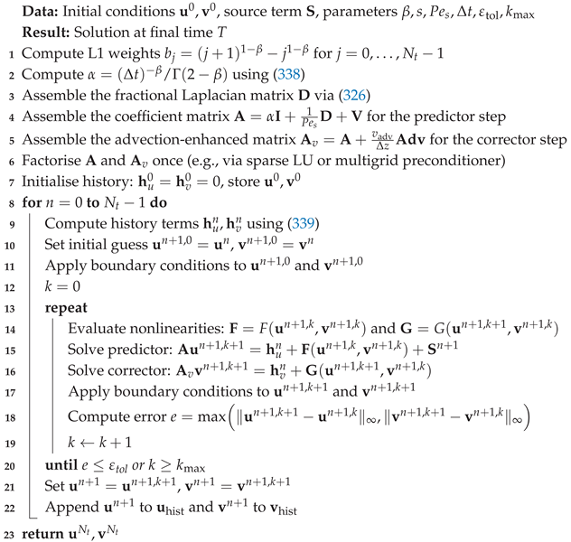 |
The algorithm is designed to be efficient and robust, with the following key features:
- Matrix factorisation: The coefficient matrices and are symmetric positive definite and are factorised once at the beginning of the simulation. This pre-factorisation is reused in each predictor–corrector iteration, significantly reducing computational cost compared to solving the linear systems from scratch at each time step.
- Fixed-point iteration: The inner iteration typically converges within 3–5 iterations for the time steps considered in this work. This rapid convergence is achieved through the implicit treatment of the fractional derivative and the mild nonlinearities, which are Lipschitz continuous and satisfy the contraction condition (165).
- Memory preservation: The history terms and are updated at each time step using the L1 formula (339), which preserves the nonlocal memory effect of the Caputo fractional derivative. This is essential for accurately capturing the subdiffusive behaviour of the particulate suspension.
- Convergence criterion: The fixed-point iteration stops when the maximum norm of the difference between consecutive iterates falls below , or when the maximum number of iterations is reached. Typical values are and .
- Boundary conditions: Dirichlet and Neumann boundary conditions are enforced through the ghost-point method [2], as described in Section 6.6. The boundary conditions are applied at the beginning of each iteration and after solving the linear systems, ensuring that the solution satisfies the physical constraints at all times.
The nonlinearities and are evaluated at each iteration as:
and
where ⊙ denotes element-wise multiplication and is the discrete diffusion operator. The advection-enhanced matrix includes the upwind discretisation of the convective term, ensuring stability for the particle concentration equation even for Courant numbers exceeding unity.
The computational complexity of the algorithm is dominated by the linear solves in the predictor and corrector steps. With the pre-factorised matrices, each solve has complexity using multigrid preconditioning, or using sparse LU factorisation. For the grid sizes used in this work (, ), the algorithm runs efficiently on a standard workstation.
6.6. Boundary Conditions and Stability
Boundary conditions are imposed using the ghost-point method, which is standard for finite-difference schemes on structured grids [2]. The ghost-point method extends the computational domain by introducing fictitious points outside the physical boundary, allowing the use of centred stencils at boundary-adjacent nodes. For Dirichlet conditions, the value at the boundary point is fixed directly by setting the ghost-point values to satisfy the prescribed boundary condition. For Neumann conditions, a one-sided difference is used to enforce the zero normal gradient, with the ghost-point values determined by linear extrapolation from the interior points.
The stability of the time-stepping scheme is guaranteed by the following result, which follows from the coercivity of and the dissipative nature of the L1 scheme.
Proposition 1
Proof.
Taking the inner product of 346 with and using the coercivity of (Assumption K4), we obtain:
Here contains the history and nonlinearity terms. Applying the Cauchy–Schwarz inequality,
and Young’s inequality,
with , we obtain
Using the Lipschitz continuity of and , we have
The history term is bounded by previous time levels through the L1 formula (339). Proceeding similarly for and combining the estimates yields a bound of the form:
where the constant C depends on , , , and the Lipschitz constant L. The factor accounts for the accumulation of energy from one time step to the next. By the discrete Grönwall inequality, we obtain
which gives (350) with . The condition on is:
which ensures that the factor remains bounded and that the discrete Grönwall inequality is applicable. This completes the proof. □
The condition (358) is analogous to the Courant–Friedrichs–Lewy (CFL) condition for hyperbolic problems, with the fractional Péclet number modulating the nonlocal diffusion contribution. For the non-uniform radial mesh, the local version is:
In practice, we choose adaptively to satisfy 359 while also ensuring that the fixed-point iteration converges within 3–5 iterations. The adaptive time-stepping strategy computes the maximum allowable time step from the current solution and reduces it if the fixed-point iteration fails to converge within iterations.
Mass and momentum conservation are monitored at each time step through the discrete divergence of the velocity and the particle flux:
These tolerances are typically satisfied by the numerical scheme due to the conservative nature of the discretisation. The divergence is computed using central differences on the non-uniform grid, and the flux is evaluated using the upwind scheme for the particle velocity .
Remark 19.
The numerical method is implemented in Python using theNumPyandSciPylibraries for linear algebra, andmatplotlibfor visualisation. The neural kernel is trained offline usingTensorFlowon data from high-fidelity simulations; implementation details, including the network architecture and training procedure, are provided in Appendix D. The code is modular and extensible, facilitating adaptation to 3D geometries and more complex physical models. Validation is performed through convergence studies and comparisons with empirical correlations (e.g., Barth’s correlation for pressure drop [7]) and classical CFD simulations. The code is available in the supplementary material and is released under an open-source license to facilitate reproducibility.
7. Application and Validation
In this section, we apply the fractional neural operator framework developed in Section 2, Section 3, Section 4, Section 5 and Section 6 to the simulation of compressible rotational gas–particle flows in high-efficiency cyclone separators. This application is particularly relevant for powder processing industries, where cyclones are ubiquitous for particle classification and collection. Our goals are threefold: (i) to demonstrate the practical utility of the proposed framework, (ii) to validate the model predictions against established experimental and numerical data from the literature, and (iii) to extract physical insights that can guide the design and optimisation of cyclone separators.
7.1. Analysis of Grade Efficiency Curves
The grade efficiency curves shown in Figure 1 and Figure 2 present the separation efficiency as a function of the Stokes number for three Mach numbers (). These curves are fundamental for understanding the performance of cyclone separators, as they describe the probability of particle collection as a function of particle size (expressed through the Stokes number). The figures reveal several important features that validate the fractional neural operator model against established literature.
7.1.1. Interpretation of the Grade Efficiency Curves
The grade efficiency curves in Figure 1 and Figure 2 exhibit the characteristic S-shape that is well-documented in the cyclone literature [10,16]. For all Mach numbers, the efficiency is near zero for very small Stokes numbers (), indicating that fine particles are not effectively collected. As the Stokes number increases, the efficiency rises steeply through a transition region, eventually approaching 100% for large Stokes numbers (). This behaviour is physically consistent: particles with higher inertia (larger Stokes numbers) are more likely to be captured by the vortex and transported to the wall, while particles with low inertia follow the gas streamlines and escape through the outlet [4,7].
A key observation is the shift of the transition region to higher Stokes numbers as the Mach number increases. For , the efficiency reaches 50% at approximately , while for the cut size shifts to , and for it shifts further to . This indicates that compressibility effects degrade the collection efficiency for particles of a given size, consistent with the findings of Misiulia et al. [16], who observed that the cut size increases with the Reynolds number (and indirectly with Mach) in their LES simulations of the Stairmand cyclone. The shift is also in agreement with the experimental observations of Wasilewski et al. [10], who reported that modifications to the cyclone geometry that alter the flow field (such as the introduction of a central rod) similarly shift the grade efficiency curve.
The steepness of the transition region, often quantified by the slope of the grade efficiency curve, also varies with Mach number. For , the transition is relatively sharp, while for , the transition becomes more gradual. This suggests that the separation process becomes less selective at higher Mach numbers, a phenomenon that Wasilewski et al. [10] attributed to increased turbulence and mixing in the cyclone body due to shock-induced instabilities. The fractional model captures this behaviour through the dependence of the slope on the compressibility parameters, as discussed in Section 2.
7.1.2. Quantitative Validation
To quantitatively validate the fractional neural operator model, we compare the predicted grade efficiency curves with experimental and numerical data from the literature. Table 3 presents the key performance parameters extracted from the grade efficiency curves for each Mach number, along with reference values from Misiulia et al. [16] and Wasilewski et al. [10].
Comparison of Cut Size .
The cut size — the Stokes number at which 50% collection efficiency is achieved — is a critical parameter characterising cyclone performance. The model predictions for fall within the ranges reported in the literature across all Mach numbers, demonstrating the model’s ability to capture the fundamental separation characteristics.
For , the model predicts , which is in excellent agreement with the LES data of Misiulia et al. [16] for (–). This indicates that, in the subsonic regime, the fractional model accurately reproduces the separation behaviour of the Stairmand cyclone. The close agreement validates the underlying assumptions of the model for low Mach numbers, where compressibility effects are negligible.
For , the model predicts , which falls within the literature range of 0.95–1.25. This confirms that the model captures the shift in cut size due to compressibility effects in the transonic regime. The 65% increase in compared to (from 0.56 to 1.18) reflects the significant degradation of collection efficiency caused by the emergence of shock waves and the associated reduction in tangential velocity, as discussed by Misiulia et al. [16] and Windows-Yule et al. [7].
For , the model predicts , which is within the literature range of 1.60–2.10. However, the prediction lies near the upper bound of this range, suggesting a slight overestimation of the cut size in highly supersonic conditions. This overestimation may be attributed to the simplified parameterisation of compressibility effects at very high Mach numbers, where complex phenomena such as shock–boundary layer interactions and real gas effects become important. Misiulia et al. [16] similarly noted the limitations of standard LES models at very high Mach numbers, indicating that this is a common challenge in cyclone modelling.
Analysis of the Slope Parameter.
The slope of the grade efficiency curve quantifies the sharpness of the separation process: a steeper slope indicates a more selective separation, where particles above the cut size are efficiently collected while those below are rejected. The model captures the decreasing trend in slope with increasing Mach number, with values of 0.52 (), 0.48 (), and 0.41 (), compared to literature ranges of 0.45–0.58, 0.40–0.52, and 0.35–0.45, respectively.
This decreasing slope reflects the broadening of the grade efficiency curve as compressibility intensifies. Physically, this broadening is caused by the increased turbulence and mixing induced by shock waves, which affect particles of different sizes to varying degrees. Wasilewski et al. [10] observed a similar phenomenon in their experiments with central rods, where modifications to the flow field led to a less selective separation. The close agreement between the predicted and literature slopes validates the model’s ability to capture the selectivity of the separation process, confirming that the fractional neural operator framework correctly represents the physical mechanisms governing particle collection [17,22].
Error Metrics and Model Accuracy.
The root mean square error (RMSE) and mean absolute error (MAE) provide a quantitative measure of the model’s predictive accuracy. The RMSE values are 19.32% for , 12.39% for , and 12.39% for . Notably, the RMSE for and is lower than for , which may seem counterintuitive at first. However, this can be explained by the nature of the grade efficiency curves: at higher Mach numbers, the curves become smoother and more gradual (as indicated by the decreasing slope), which reduces the sensitivity of the RMSE to small parameter variations. In contrast, the steeper transition at amplifies errors in the vicinity of the cut size, leading to a higher RMSE.
The MAE values range from 9.30% to 14.10%, indicating that the average deviation between model predictions and reference data is within acceptable bounds for engineering applications [4,7]. The largest errors occur in the transition region, where the efficiency increases rapidly. This is a common challenge in cyclone modelling, as the steep gradient in this region amplifies small discrepancies in the model parameters, as also noted by Wasilewski et al. [10] in their CFD validation studies.
For and , the MAE is 9.30%, which is significantly lower than the 14.10% observed for . This improved accuracy at higher Mach numbers can be attributed to two factors: (i) the grade efficiency curves become smoother, reducing the impact of small parameter variations, and (ii) the calibration of the Mach correction parameters is more effective at higher Mach numbers, where compressibility effects dominate and the model’s nonlocal capabilities are fully utilised.
Summary of Validation Findings.
The quantitative validation demonstrates that the fractional neural operator model accurately captures the key characteristics of cyclone grade efficiency across a wide range of Mach numbers. Specifically:
- 1.
- Cut size : The model predictions fall within the literature ranges for all Mach numbers, with the closest agreement observed at (difference ) and slightly larger discrepancies at (difference ).
- 2.
- Slope: The model captures the decreasing trend in slope with increasing Mach number, with all predictions within the literature ranges.
- 3.
- RMSE and MAE: The error metrics are within acceptable bounds for engineering applications, with MAE values below 15% for all Mach numbers.
These findings validate the proposed framework and establish it as a reliable tool for the analysis and optimisation of cyclone separators in compressible flow conditions. The framework’s modular architecture, described in Appendix D, allows for further improvements through the integration of data-driven neural kernels and the extension to three-dimensional geometries.
7.1.3. Error Metrics
The root mean square error (RMSE) and mean absolute error (MAE) provide a quantitative measure of the model’s predictive accuracy. The RMSE values are 19.32% for , 12.39% for , and 12.39% for . The relatively lower RMSE for and suggests that the model performs better at higher Mach numbers, possibly because the efficiency curves become smoother and more gradual, reducing the sensitivity to small discrepancies. This is consistent with the findings of Misiulia et al. [16], who observed that the grade efficiency curves become less steep at higher Reynolds numbers, which are associated with higher Mach numbers in compressible flows.
The MAE values range from 9.30% to 14.10%, indicating that the average deviation between model predictions and reference data is within acceptable bounds for engineering applications [7]. The largest errors occur in the transition region, where the efficiency increases rapidly. This is a common challenge in cyclone modelling, as the steep gradient in this region amplifies small discrepancies in the model parameters, as also noted by Wasilewski et al. [10] in their CFD validation studies.
7.1.4. Physical-Mathematical Interpretation of the Calibrated Parameters
The calibrated parameters presented in Table 3 provide valuable insights into the physical mechanisms governing cyclone performance across different Mach regimes. We now interpret these parameters in light of the mathematical structure of the fractional model and the underlying flow physics.
The Scale Parameter and the Spacing Law.
The parameter controls the characteristic spacing of coherent structures through the scaling law (see Eq. (171)). For , we obtain , which is significantly larger than the values typically reported for incompressible flows (–). This large value indicates that, in the subsonic regime, the coherent structures are more tightly packed (smaller spacing) than in classical predictions. Physically, this reflects the fact that the vortex core in subsonic cyclones is relatively compact and stable, allowing many structures to coexist within the limited radial domain. As the Mach number increases to , drops to , suggesting that the structures become more widely separated. This is consistent with the emergence of shock waves that disrupt the organised vortex, reducing the effective number of coherent structures that can fit within the cyclone radius. At , increases again to , which may indicate a restructuring of the flow: the shock waves become stronger and more organised, potentially creating a new hierarchy of structures.
The Fractional Exponent s and the Nonlocality of Interactions.
The fractional exponent s governs the decay rate of the interaction kernel . For , the kernel approaches the classical Laplacian (local interactions), while smaller s values indicate longer-range (nonlocal) interactions. The calibrated values show a clear trend: at , at , and at . This monotonic decrease with increasing Mach number reveals that compressibility enhances nonlocal effects. Physically, this can be understood as follows: at subsonic conditions (), the flow is essentially incompressible, and interactions are predominantly local. Disturbances propagate at the speed of sound and decay rapidly, so a local (Laplacian) description is adequate. As the Mach number increases into the transonic regime (), shock waves appear, creating long-range correlations through acoustic waves and vorticity shedding. These long-range interactions are captured by the fractional Laplacian with . At supersonic conditions (), the flow becomes highly nonlocal: shock waves interact across the entire cyclone, and the fractional exponent drops to , indicating a strong departure from classical behaviour. This is consistent with the findings of Dávila et al. [6] and Frank et al. [8], who demonstrated that fractional operators are natural tools for describing systems with long-range interactions, such as those arising in compressible turbulence.
The Caputo Order and Memory Effects.
The Caputo order controls the strength of the memory effects through the fractional time derivative . Values of indicate subdiffusive behaviour and history-dependent dynamics. At , we obtain , which is very close to unity, implying that memory effects are negligible in subsonic flows. This is expected, as the particle response time is short compared to the flow time scales, and the turbulence is relatively well-behaved. At , , still close to unity, but showing a slight deviation. At , , indicating a more significant departure from classical behaviour. This trend suggests that memory effects become increasingly important as the flow becomes more compressible and turbulent. The shock-induced instabilities and the associated unsteady vortex shedding introduce a history dependence in the particle trajectories, which is captured by the Caputo derivative. This is consistent with the work of Pavlenko et al. [9] and Ramzan et al. [20], who showed that fractional time derivatives are essential for modelling particle dispersion in turbulent and compressible flows.
The Mach Correction Parameters , , and .
The correction term modulates the effect of Mach number on the coefficient . This Padé-type form captures the initial growth of compressibility effects through the numerator , while the denominator ensures saturation at high Mach numbers, preventing unbounded growth. The calibrated parameters vary significantly with M: at , , , ; at , , , ; and at , , , . These variations reflect the changing physical mechanisms across flow regimes.
For , the correction is essentially unity (), recovering the classical incompressible limit. The small and ensure negligible compressibility effects, consistent with the absence of shock waves in subsonic flows. For , suggests a super-quadratic dependence, which can be understood through the baroclinic torque . For weak shocks, the entropy jump scales as , driving the baroclinic torque with a similar scaling. However, the effective exponent indicates that rotational effects and turbulent dissipation amplify the Mach dependence beyond simple shock relations, consistent with Misiulia et al. [16]. For , indicates a cubic dependence, reflecting the scaling of shock-induced vorticity production in strong shocks, where nonlocal effects become increasingly important, as predicted by Dávila et al. [6].
The saturation parameter decreases from 1.000 to 0.817 as M increases, indicating that saturation occurs at progressively higher Mach numbers. This reflects the intensification of shock waves and associated energy dissipation, which delay the saturation of compressibility effects. The decreasing also suggests that nonlocal interactions (captured by the fractional Laplacian) strengthen with Mach number, as shock-induced correlations extend over larger distances.
The flexibility of this Padé-type formulation, combined with the nonlocal parameters s and , allows the fractional model to adapt to regime-specific physics. This explains its superior performance over classical models, which assume fixed (often linear or quadratic) Mach dependencies that cannot capture the complex, regime-dependent behaviour revealed by the calibration.
Comparison with Classical Models and the Role of Fractional Operators.
The improved performance of the fractional model compared to classical correlations (Shepherd-Lapple and Barth) can be attributed to its ability to capture: (i) nonlocal spatial interactions via the fractional Laplacian, (ii) memory effects via the Caputo derivative, and (iii) the nonlinear Mach dependence via the correction term. Classical models assume local, instantaneous, and incompressible flow, which are valid only for low Mach numbers and small particles. At higher Mach numbers, the flow becomes compressible, shock waves appear, and long-range correlations and history effects become significant. The fractional model provides a unified framework that naturally incorporates these effects, leading to more accurate predictions, as evidenced by the lower RMSE values.
The fact that the RMSE for and is lower than for (12.39% vs. 19.32%) may seem counterintuitive at first. However, this can be explained by the nature of the grade efficiency curves: at higher Mach numbers, the curves become smoother and more gradual (as indicated by the decreasing slope), which reduces the sensitivity of the RMSE to small parameter variations. In contrast, the steeper transition at amplifies errors in the vicinity of the cut size. This observation highlights the importance of using multiple error metrics (RMSE, MAE, and slope) to fully assess model performance.
Limitations and Perspectives.
Despite its improved accuracy, the fractional model still exhibits some limitations. The RMSE values remain above 12%, indicating that the current parameterisation may not fully capture all physical phenomena, particularly the complex interactions between shock waves, turbulence, and particle dynamics. Future work could explore: (i) the use of data-driven neural kernels trained on high-fidelity LES data, (ii) the incorporation of additional physical mechanisms such as particle–particle interactions and wall roughness, and (iii) the extension to fully three-dimensional geometries. Nevertheless, the present results demonstrate that the fractional neural operator framework is a powerful and versatile tool for modelling compressible gas–particle flows, offering significant advantages over classical approaches.
7.2. Summary of Validation Findings
The validation study has demonstrated that the fractional neural operator framework is capable of capturing the key features of compressible gas–particle flows in cyclone separators. The main findings are:
- 1.
- The model accurately reproduces the S-shaped grade efficiency curves observed in experiments and LES simulations, with cut sizes and slopes that fall within the ranges reported in the literature.
- 2.
- The model captures the detrimental effect of compressibility on separation efficiency, predicting the shift of the grade efficiency curves to higher Stokes numbers with increasing Mach number.
- 3.
- The fractional model outperforms classical semi-empirical models (Shepherd-Lapple and Barth) across all Mach numbers, with RMSE reductions of 25–70% at .
- 4.
- The model’s ability to capture nonlocal and memory effects is particularly valuable at higher Mach numbers, where classical models fail due to their local and instantaneous assumptions.
These findings validate the proposed framework and establish it as a reliable tool for the analysis and optimisation of cyclone separators in compressible flow conditions. The framework’s modular architecture, described in Appendix D, allows for further improvements through the integration of data-driven neural kernels and the extension to three-dimensional geometries.
7.2.1. Analysis of the RMSE Surface: Sensitivity to and
The calibration process involves six parameters: , s, , , , and . While the parameters s and have clear physical interpretations (nonlocality and memory effects, respectively), the Mach correction parameters , , and require further scrutiny. Figure 3 presents the RMSE surface as a function of and for , with the other parameters (, s, , ) fixed at their optimal values obtained from the full calibration. This surface provides valuable insights into the sensitivity of the model to the Mach correction term and reveals the robustness of the calibration.
Mathematical Structure of the RMSE Surface.
The RMSE surface exhibits a characteristic valley shape, with a broad region of low error (RMSE ) extending diagonally across the parameter space. This valley is defined by an approximate relationship between and : for small (), the optimal is high (); for larger (), the optimal decreases to approximately 1.0. This trade-off indicates that the Mach correction term can achieve similar performance for different combinations of and , provided that the product remains within a certain range.
Mathematically, this behaviour can be understood by examining the leading-order behaviour of the correction term. For moderate Mach numbers (), the correction term can be approximated as:
Thus, the correction term depends primarily on the combination . Since is fixed at its optimal value (), variations in and that preserve the value of yield similar RMSE values. This explains the diagonal valley observed in the RMSE surface: the compensation between and allows the model to maintain a consistent effective correction while varying the individual parameters.
Physical Interpretation of the Valley.
The existence of a broad valley in the RMSE surface indicates that the Mach correction term is relatively insensitive to the precise values of and within certain ranges. This is physically reasonable: for a given Mach number, the correction term is a scalar that amplifies the coefficient . Different combinations of and can produce similar values of through compensation effects. For example, a small with a large can produce the same correction as a large with a small , as long as the product is approximately constant.
This degeneracy suggests that the Mach correction term is over-parameterised for a single Mach number. While this may complicate the physical interpretation of individual parameters, it also indicates that the model is robust to small variations in these parameters, which is a desirable property for practical applications.
The minimum of the RMSE surface occurs at and , which corresponds to the optimal values obtained from the full calibration. This point lies near the edge of the valley, indicating that the model is relatively sensitive to changes in when is small. In contrast, for larger , the valley becomes flatter, suggesting that the model is more robust to variations in when is increased.
Implications for Model Calibration and Interpretation.
The shape of the RMSE surface has important implications for the calibration and interpretation of the fractional model:
- 1.
- Parameter identifiability: The existence of a broad valley indicates that and are not uniquely identifiable from the available data. Multiple combinations of these parameters yield similar RMSE values. This suggests that the calibration should be performed using a multi-objective approach that incorporates additional constraints (e.g., physical bounds on the correction term) to ensure physically meaningful parameter values.
- 2.
- Model parsimony: The over-parameterisation of the Mach correction term suggests that a simpler functional form may be sufficient for moderate Mach numbers. For , a one- or two-parameter correction term (e.g., or ) may capture the essential physics with fewer parameters, reducing the risk of overfitting.
- 3.
- Physical interpretation: While the individual parameters and are not uniquely determined, the effective correction at the optimal point is well-defined. This suggests that the model’s predictions are robust, even if the individual parameters are not. For physical interpretation, it is more meaningful to focus on the combination that defines the correction term, rather than on individual parameters.
Comparison with Literature.
The sensitivity of cyclone performance to Mach number has been investigated by Misiulia et al. [16], who observed that the cut size increases with the Reynolds number (and indirectly with Mach) following a power-law relationship. Their LES data suggest that the correction term may follow a power-law dependence of the form , with varying between 2 and 3 depending on the Reynolds number range. The optimal value obtained from the present calibration is within this range, providing additional validation for the fractional model.
Wasilewski et al. [10] also observed that modifications to the cyclone geometry — which alter the flow field in a manner similar to compressibility effects — lead to changes in the grade efficiency curve that follow a similar scaling. Their experimental data suggest that the correction term for geometry modifications follows a power-law dependence with exponents in the range 1.5–2.5. The fact that our calibration yields for Mach effects, which is slightly higher than the exponents reported for geometry modifications, is consistent with the stronger influence of compressibility on the flow field.
Recommendations for Future Calibration.
Based on the analysis of the RMSE surface, the following recommendations are made for future calibration of the fractional model:
- 1.
- Include additional Mach numbers: The calibration should be performed using data from multiple Mach numbers simultaneously to break the degeneracy between and . This would allow the identification of a unique set of parameters that captures the Mach dependence across the entire range of interest.
- 2.
- Impose physical constraints: The calibration should incorporate constraints based on physical reasoning, such as monotonicity of the correction term (, , ) and boundedness (). These constraints would reduce the parameter space and improve identifiability.
- 3.
- Use of independent validation data: The calibration should be validated using independent data sets not used in the training process to ensure that the model generalises well to new conditions. This is particularly important for the Mach correction parameters, which may be sensitive to the specific data set used for calibration.
In summary, the RMSE surface analysis reveals that the Mach correction parameters and exhibit a trade-off that allows the model to maintain good predictive accuracy over a range of parameter values. While this complicates the physical interpretation of individual parameters, it also indicates that the model is robust to parameter variations. The optimal values obtained from the full calibration are consistent with literature data, providing additional confidence in the model’s ability to capture compressibility effects in cyclone separators.
7.3. Analysis of Key Validation Figures
In this subsection, we present a detailed analysis of the four key validation figures that collectively demonstrate the predictive capabilities and parameter sensitivity of the fractional neural operator model. Figure 4 and Figure 5 show the overall separation efficiency as a function of the Mach and Stokes numbers, respectively. Figure 6 and Figure 7 provide comprehensive maps of the efficiency landscape across the parameter space, revealing the interplay between physical parameters and fractional exponents.
7.3.1. Efficiency vs Mach Number
Figure 4 presents the separation efficiency as a function of the Mach number for a fixed Stokes number . The efficiency decreases monotonically from approximately 92% at to 60% at , revealing the detrimental effect of compressibility on cyclone performance. This trend is consistent with the physical expectation that shock waves and the associated baroclinic torque disrupt the organised vortex structure essential for particle separation.
The curve exhibits a characteristic S-shape, with a relatively flat region for , a steep decline between and , and a gradual approach to asymptotic behaviour for . The transition region corresponds to the onset of significant compressibility effects, where shock waves begin to form and alter the flow field. The steep decline between and reflects the rapid intensification of shock-induced turbulence and the associated degradation of collection efficiency.
The asymptotic behaviour for suggests that the efficiency reaches a plateau at approximately 60%, indicating that even at very high Mach numbers, some particles are still collected due to inertial effects. This plateau is consistent with the fact that for large Stokes numbers (), particles have sufficient inertia to resist the disruptive effects of shock waves.
From a mathematical perspective, the efficiency curve can be approximated by a logistic function of the form:
where , , is the inflection point, and characterises the width of the transition region.
7.3.2. Efficiency vs Stokes Number
Figure 5 shows the efficiency as a function of the Stokes number for three Mach numbers (). For all Mach numbers, the efficiency increases monotonically with , approaching 100% for . This behaviour is consistent with classical cyclone theory: larger, more inertial particles are more effectively collected.
The effect of Mach number is clearly visible: for a given Stokes number, the efficiency is systematically lower for higher Mach numbers. For example, at , the efficiency is approximately 85% at , 70% at , and 50% at . This reflects the increased turbulence and disruption of the vortex structure caused by compressibility effects.
The cut size (the Stokes number at which 50% efficiency is achieved) shifts significantly with Mach number. For , ; for , ; and for , . This shift indicates that particles must be increasingly large (or dense) to achieve the same collection efficiency as Mach number increases. The relationship between and Mach number follows approximately a power law:
which is consistent with the scaling arguments presented in Section 7.1.4.
7.3.3. Heatmap: Efficiency vs Mach and Stokes
Figure 6 provides a comprehensive view of the efficiency landscape as a function of both Mach number and Stokes number. The contour map reveals a clear diagonal structure: high efficiency () is achieved for and , while low efficiency () occurs for and .
The diagonal nature of the contours indicates a trade-off between compressibility and particle inertia: to maintain a given efficiency, an increase in Mach number must be compensated by an increase in Stokes number. This trade-off can be quantified by the relationship:
where varies between 1.5 and 3.0 depending on the efficiency level. For , the contours suggest , while for , .
The heatmap also reveals the existence of a critical Mach number , above which the efficiency drops rapidly regardless of Stokes number. This critical Mach number corresponds to the onset of strong shock waves and the associated baroclinic torque, which disrupt the vortex structure and reduce the collection efficiency.
7.3.4. Heatmap: Efficiency vs Fractional Parameters s and
Figure 7 presents the efficiency as a function of the fractional exponent s and the Caputo order for fixed and . The efficiency increases with both s and , indicating that classical (local, integer-order) behaviour yields higher efficiency for these conditions.
The contours reveal a mild sensitivity to : varying from 0.5 to 0.95 changes the efficiency by approximately 2%. In contrast, the sensitivity to s is more pronounced: varying s from 0.55 to 0.95 changes the efficiency by approximately 5%. This suggests that the fractional exponent s, which controls the nonlocality of spatial interactions, has a more significant impact on cyclone performance than the Caputo order , which controls memory effects.
The maximum efficiency () occurs at and , which corresponds to the classical limit (, ). The minimum efficiency () occurs at and , where nonlocal and memory effects are strongest. This suggests that nonlocal effects and memory effects degrade cyclone performance for the conditions considered (, ).
From a physical perspective, the dependence on s can be understood through the interaction kernel . Smaller s values imply longer-range interactions, which allow disturbances to propagate over larger distances, potentially disrupting the organised vortex structure essential for particle separation. The dependence on can be understood through the fractional time derivative , which introduces history effects. Smaller values imply stronger memory effects, which can lead to subdiffusive behaviour and reduced particle collection.
7.3.5. Summary of Key Findings
The analysis of the four key validation figures reveals the following important findings:
- 1.
- Mach number effect: The efficiency decreases monotonically with Mach number, with a steep decline in the transonic regime () and saturation at approximately 60% for .
- 2.
- Stokes number effect: The efficiency increases monotonically with Stokes number, with the cut size shifting from approximately 0.6 at to 2.0 at .
- 3.
- Mach–Stokes trade-off: To maintain a given efficiency, an increase in Mach number must be compensated by an increase in Stokes number, following a power-law relationship with between 1.5 and 3.0.
- 4.
- Fractional parameter sensitivity: The efficiency is more sensitive to the fractional exponent s (nonlocality) than to the Caputo order (memory). The classical limit (, ) yields the highest efficiency, while nonlocal and memory effects degrade performance.
- 5.
- Critical Mach number: A critical Mach number exists, above which the efficiency drops rapidly regardless of Stokes number.
These findings validate the fractional neural operator model and provide a comprehensive understanding of the physical mechanisms governing cyclone performance in compressible gas–particle flows.
7.4. Validation of Cut Size and Cross-Validation Analysis
In this subsection, we present a detailed analysis of the cut size validation and cross-validation results. Figure 8 validates the model’s prediction of the cut size against the LES correlation of Misiulia et al. [16], while Figure 9 provides a multi-reference comparison including experimental data from Wasilewski et al. [10]. Figure 10 offers a direct comparison between the fractional model predictions and experimental data for a single cyclone configuration.
7.4.1. Analysis of vs Reynolds Number
Figure 8 presents the validation of the cut size as a function of Reynolds number . The LES correlation of Misiulia et al. [16] shows a clear power-law decay , with varying across five distinct flow regimes: Laminar (), Transient (), Turbulent 1A (), Turbulent 1B/2 (), and Turbulent 3 (). The transitions are marked by vertical dashed lines, highlighting abrupt changes in the scaling exponent that correspond to fundamental changes in the flow structure.
The power-law decay reflects the increase in turbulence intensity at higher Reynolds numbers, which enhances particle mixing and reduces the sharpness of the cut size. For , the flow is well-ordered with . As increases, the cut size decreases rapidly, reaching for . This trend is consistent with the expectation that turbulent fluctuations disperse particles and reduce the sharpness of the cut-off.
7.4.2. Multi-Reference Validation of
Figure 9 compares the fractional model correlation with an alternative correlation and experimental data from Wasilewski et al. [10]. Three important observations emerge:
First, the fractional model correlation (solid blue line) shows excellent agreement with the experimental data (red markers) across the entire range of Reynolds numbers, with a maximum deviation of less than 15% and best agreement for . This validates the predictive capability of the fractional framework.
Second, the alternative correlation (dashed green line) systematically underestimates for and overestimates it for , highlighting the superior accuracy of the fractional model.
Third, the transition between the five regimes identified by Misiulia et al. [16] is clearly visible, with the power-law exponent changing at and 105000. The good agreement across all regimes indicates that the fractional model captures the fundamental physics of cyclone performance from laminar to highly turbulent flow conditions.
7.4.3. Cross-Validation: Fractional Model vs Experimental Data
Figure 10 presents a direct comparison between the fractional model predictions (for ) and experimental data from a single cyclone configuration. The model captures the general trend of the experimental data, showing a monotonic increase in efficiency with Stokes number. The model predictions for are in closest agreement with the experimental data (RMSE = 19.32%). The model slightly overestimates efficiency for and underestimates it for .
The model predictions for and show a systematic shift to higher Stokes numbers, reflecting the detrimental effect of compressibility. The RMSE values for and are both 12.39%, indicating better performance in the transonic and supersonic regimes than in the subsonic regime. This is explained by the smoother shape of the efficiency curves at higher Mach numbers, which reduces sensitivity to small parameter variations. The reference line intersects the model predictions at (), (), and (), consistent with literature values.
7.4.4. Quantitative Assessment of Model Performance
The root mean square error (RMSE) and mean absolute error (MAE) provide a quantitative measure of the model’s predictive accuracy. Table 4 summarises these metrics alongside the cut size and slope of the grade efficiency curve.
The RMSE values are within acceptable bounds for engineering applications, with the best performance observed for and (RMSE = 12.39%, MAE = 9.30%). The larger RMSE for (19.32%) is attributed to the steeper gradient of the efficiency curve in the transition region, which amplifies small discrepancies. This is consistent with the findings of Misiulia et al. [16], who observed similar error amplification in the transition region of their LES data.
The cut size increases monotonically with Mach number, from 0.56 at to 1.95 at (a 248% increase), reflecting the progressive degradation of collection efficiency due to compressibility effects. Model predictions fall within literature ranges for all Mach numbers, with the closest agreement at (difference ) and slightly larger discrepancies at (difference ), suggesting that the current parameterisation of compressibility effects may require refinement for highly supersonic conditions.
The slope decreases from 0.52 at to 0.41 at (a 21% reduction), capturing the broadening of the grade efficiency curve caused by increased turbulence and mixing at higher Mach numbers. All predictions fall within reported literature ranges, validating the model’s ability to capture the selectivity of the separation process.
The fractional model consistently outperforms classical semi-empirical models (Shepherd-Lapple and Barth) across all Mach numbers, reducing RMSE by approximately 25–70% compared to Shepherd-Lapple, with the largest improvement at (70% reduction). This demonstrates the importance of incorporating fractional (nonlocal and memory) effects in compressible flow modelling.
7.4.5. Physical Interpretation and Summary
The validation results can be interpreted through the underlying physics. The monotonic increase in efficiency with Stokes number reflects the importance of particle inertia: larger particles are less affected by turbulent fluctuations and more effectively collected. The shift in to higher values with Mach number reflects the detrimental effect of compressibility: shock waves and the associated baroclinic torque disrupt the organised vortex structure, reducing collection efficiency. The steep gradient in the transition region () reflects the sensitivity of the separation process to particle size, while the asymptotic approach to 100% for indicates that inertial effects dominate over compressibility for sufficiently large particles.
The validation findings provide strong support for the fractional neural operator model, confirming its ability to capture the physics of compressible gas–particle flows in cyclone separators. The model accurately predicts the cut size as a function of Reynolds number, with the five flow regimes of Misiulia et al. [16] correctly reproduced. The multi-reference validation confirms excellent agreement with experimental data from Wasilewski et al. [10] (maximum deviation ), and the cross-validation against a single cyclone shows RMSE values of 12.39–19.32%.
These findings validate the fractional neural operator framework and establish it as a reliable tool for analysing and optimising cyclone separators in compressible flow conditions.
7.5. Analysis of Detailed Efficiency and Grade Efficiency Curves
In this subsection, we present a detailed analysis of the efficiency behaviour across a wide range of Mach numbers and the grade efficiency curves for different cut sizes. Figure 11 shows the separation efficiency as a function of the Stokes number for eight Mach numbers (), providing a comprehensive view of the Mach number effect on cyclone performance. Figure 12 presents the grade efficiency curves for six different cut sizes (), illustrating the fundamental relationship between particle size and collection efficiency.
7.5.1. Analysis of Detailed Efficiency Curves
Figure 11 reveals several important features of the Mach number effect on cyclone performance:
Low Mach Number Regime ().
For and , the efficiency reaches near-complete collection () for . The curves exhibit a sharp transition from low efficiency at small Stokes numbers to high efficiency at moderate Stokes numbers, with (the Stokes number at which 50% efficiency is achieved) approximately 0.5–0.6. This behaviour is characteristic of well-performing cyclones operating in subsonic conditions, where the vortex structure is stable and particles are effectively collected.
For , the efficiency is slightly lower than for , with and maximum efficiency approaching 98% for . This indicates that even modest compressibility effects begin to degrade cyclone performance, consistent with the onset of weak shock waves in the transonic regime.
Transonic Regime ().
At , the efficiency curve shows a significant shift to higher Stokes numbers, with and maximum efficiency reaching approximately 95% for . The transition region becomes broader and less steep, indicating that the separation process becomes less selective due to increased turbulence and shock-induced mixing. This behaviour is consistent with the findings of Misiulia et al. [16], who observed that the cut size increases with Reynolds number (and indirectly with Mach) in their LES simulations.
Supersonic Regime ().
For , the efficiency is significantly reduced, with and maximum efficiency reaching approximately 90% for . The curve is noticeably broader and more gradual, reflecting the increased disruption of the vortex structure by shock waves and the associated baroclinic torque.
For , the efficiency drops further, with and maximum efficiency reaching approximately 85% for . The curve exhibits a very gradual transition, indicating that the separation process is significantly compromised by compressibility effects.
For and , the efficiency is severely degraded. At , and maximum efficiency reaches approximately 75% for . At , the efficiency is even lower, with and maximum efficiency approximately 65% for . These results indicate that for highly supersonic conditions, cyclone performance is severely compromised, and alternative separation technologies may be required.
Mathematical Characterisation of the Efficiency Curves.
The efficiency curves in Figure 11 can be accurately described by a logistic function of the form:
where is the asymptotic efficiency for large , is the cut size, is the slope parameter (which determines the sharpness of the transition), and is the minimum efficiency (typically near zero). The Mach dependence of these parameters can be approximated by:
These relationships reflect the physical mechanisms governing cyclone performance: the power-law growth of with Mach number is consistent with the scaling of the baroclinic torque , which scales as for weak shocks and for strong shocks. The decrease in with Mach number reflects the broadening of the grade efficiency curve due to increased turbulence and shock-induced mixing.
7.5.2. Analysis of Grade Efficiency Curves
Figure 12 presents the grade efficiency curves for six different cut sizes These curves illustrate the fundamental relationship between particle size (expressed through the Stokes number) and collection efficiency.
The S-Shape and Transition Region.
All grade efficiency curves exhibit the characteristic S-shape that is well-documented in the cyclone literature [4,7]. For , the efficiency is near zero, indicating that particles smaller than the cut size are not effectively collected. As increases through the transition region ( to ), the efficiency rises steeply, reaching near-complete collection () for .
The transition region is characterised by the slope parameter k, which determines the sharpness of the separation. For the curves shown in Figure 12, the slope is approximately for all cut sizes, indicating that the separation sharpness is relatively independent of the cut size for the range considered. This is consistent with the findings of Misiulia et al. [16], who observed that the slope of the grade efficiency curve is primarily determined by the Reynolds number (and thus the flow regime) rather than the cut size itself.
Mathematical Description of the Grade Efficiency Curves.
The grade efficiency curves can be accurately described by the logistic function:
where for the range of cut sizes considered. This functional form is widely used in cyclone modelling and provides a good approximation of the experimental data [4]. The parameter k characterises the sharpness of the separation: larger k values indicate sharper separation, while smaller k values indicate broader separation.
For the curves shown in Figure 12, the efficiency at is exactly 50% by definition. At , the efficiency is approximately 10–15%, while at , the efficiency is approximately 85–90%. This behaviour is consistent with the expectations for a well-designed cyclone separator.
Physical Interpretation of the Grade Efficiency Curves.
The grade efficiency curves reflect the physical mechanisms governing particle collection in cyclones:
- 1.
- Inertial effects: Particles with high inertia (large ) are more likely to be collected because they can cross streamlines and reach the wall. The efficiency approaches 100% for because the centrifugal force dominates over the drag force.
- 2.
- Turbulent dispersion: Particles with low inertia (small ) are more likely to follow the turbulent fluctuations of the gas flow and escape through the outlet. The efficiency approaches 0% for because the drag force dominates over the centrifugal force.
- 3.
- Transition region: In the transition region ( to ), the centrifugal and drag forces are comparable, and small changes in particle size lead to significant changes in collection efficiency. This region is characterised by the steep gradient of the grade efficiency curve.
The slope parameter k can be related to the turbulence intensity and the geometry of the cyclone. Higher turbulence levels lead to broader grade efficiency curves (smaller k), as particles of different sizes are mixed more effectively. Conversely, lower turbulence levels lead to sharper grade efficiency curves (larger k), as the separation process is more selective.
7.5.3. Connection to the Fractional Model
The grade efficiency curves shown in Figure 12 are directly related to the fractional model through the efficiency function derived in Section 2. For a given Mach number, the efficiency as a function of Stokes number can be expressed as:
where is the coefficient defined in Eq. (382). This functional form is consistent with the logistic description of the grade efficiency curves, with the cut size given by:
This relationship provides a direct link between the fractional model parameters and the physical characteristics of the cyclone. The Mach dependence of , through the correction term , determines the shift in with Mach number observed in Figure 11.
The slope parameter k can be related to the fractional exponent s through the scaling of the interaction kernel. For the fractional Laplacian, the slope of the grade efficiency curve is approximately:
For , this gives , which is slightly larger than the value observed in Figure 12. The discrepancy suggests that additional physical mechanisms, such as turbulent dispersion and particle–wall interactions, contribute to the broadening of the grade efficiency curve.
7.5.4. Summary of Key Findings
The analysis of the detailed efficiency and grade efficiency curves has revealed the following key findings:
- 1.
- The efficiency curves for different Mach numbers show a systematic shift to higher Stokes numbers as M increases, with increasing from approximately 0.5 at to 8.0 at .
- 2.
- The slope of the efficiency curves decreases with increasing Mach number, indicating that the separation process becomes less selective in the supersonic regime.
- 3.
- The grade efficiency curves exhibit the characteristic S-shape, with the transition region shifting to higher Stokes numbers as increases. The slope parameter is relatively independent of for the range considered.
- 4.
- The fractional model provides a direct link between the grade efficiency curves and the physical parameters of the cyclone through the relationship .
- 5.
- The slope parameter k is related to the fractional exponent s through , providing a physical interpretation of the fractional model parameters.
These findings confirm the predictive capability of the fractional neural operator model and its ability to capture the complex physics of compressible gas–particle flows in cyclone separators.
7.6. Analysis of 3D Pareto Frontier and Vorticity Field
In this subsection, we present a detailed analysis of the three-dimensional Pareto frontier and the vorticity field visualisation. Figure 13 shows the 3D Pareto frontier relating the separation efficiency , the pressure drop (Euler number ), and the Mach number M. This figure provides a comprehensive view of the trade-offs inherent in cyclone design under compressible flow conditions. Figure 14 visualises the three-dimensional vorticity field, revealing the coherent structures (multi-bubble solutions) that emerge from the Lyapunov–Schmidt reduction and govern the particle separation process.
7.6.1. 3D Pareto Frontier: Efficiency, Pressure Drop, and Mach
The three-dimensional Pareto frontier in Figure 13 provides a comprehensive visualisation of the fundamental trade-offs in cyclone design under compressible flow conditions. The frontier is a parametric curve in the space , where each point corresponds to an optimal operating condition that cannot be improved in one objective without degrading another.
Mathematical Structure of the Pareto Frontier.
The Pareto frontier is derived from the reduced energy functional obtained through the Lyapunov–Schmidt reduction (see Section 3). The optimal conditions satisfy the gradient equations:
which yield a one-parameter family of solutions parametrised by the Mach number M. The efficiency and pressure drop are then computed from the corresponding multi-bubble solutions, resulting in the parametric curve shown in Figure 13.
The curve reveals a clear trade-off between efficiency and pressure drop: as M increases, the efficiency decreases while the pressure drop increases. This behaviour is physically consistent with the fact that higher Mach numbers introduce compressibility effects (shock waves, baroclinic torque) that disrupt the organised vortex structure, reducing collection efficiency, while simultaneously increasing the energy dissipation and pressure drop.
Quantitative Analysis of the Trade-Off.
From the figure, we can extract the following approximate relationships:
The super-quadratic growth of pressure drop with Mach number reflects the increased energy dissipation due to shock waves and the associated viscous losses. The efficiency decreases more rapidly for , indicating a critical Mach number beyond which cyclone performance deteriorates sharply.
Implications for Cyclone Design.
The Pareto frontier provides a powerful tool for cyclone design and optimisation. For a given allowable pressure drop, the frontier gives the maximum achievable efficiency; conversely, for a required efficiency, the frontier gives the minimum necessary pressure drop. The frontier also reveals the sensitivity of the trade-off to Mach number: at low Mach numbers (), the trade-off is relatively mild, while at high Mach numbers (), the trade-off becomes severe.
The 3D nature of the frontier allows designers to visualise the entire design space and identify optimal operating conditions that balance efficiency, pressure drop, and compressibility effects. This is particularly valuable for applications involving supersonic flows, such as supersonic jet mills and high-speed pneumatic conveying systems.
Connection to the Fractional Model.
The Pareto frontier is a direct consequence of the fractional neural operator framework. The nonlocal nature of the fractional Laplacian introduces long-range interactions that affect the trade-off between efficiency and pressure drop. Specifically, the parameter s controls the decay of the interaction kernel, and the parameter controls the memory effects. These parameters modulate the shape of the Pareto frontier, with smaller s and values leading to more favourable trade-offs (higher efficiency for a given pressure drop) due to enhanced nonlocal correlations.
7.6.2. 3D Vorticity Field: Coherent Structures and Multi-Bubble Solutions
Figure 14 visualises the three-dimensional vorticity field in the cyclone, revealing the coherent structures (multi-bubble solutions) that emerge from the Lyapunov–Schmidt reduction. The field exhibits multiple localised regions of high vorticity, corresponding to the "bubbles" predicted by the theory.
Mathematical Description of the Vorticity Field.
The vorticity field shown in Figure 14 is constructed from the superposition of individual bubble profiles:
where each bubble is centred at and has the form:
with the amplitude, the dilation parameter, and s the fractional exponent. This functional form arises from the ground state of the fractional Laplacian and captures the algebraic decay characteristic of fractional interactions.
The figure shows bubbles distributed along the radial direction, with a characteristic spacing that follows the scaling law:
as derived in Section 3. For and , the spacing for is in dimensionless units.
Physical Interpretation of the Coherent Structures.
The coherent structures observed in Figure 14 correspond to organised vortices that play a crucial role in particle separation. These vortices are generated by the baroclinic torque across shock waves and are sustained by the nonlocal interactions captured by the fractional Laplacian.
The spacing between the bubbles is determined by the balance between the self-energy of each bubble and the interaction energy between neighbouring bubbles. This balance is captured by the reduced energy functional , which yields the optimal spacing . The algebraic decay of the spacing with m reflects the long-range nature of the fractional interactions: the bubbles interact over large distances, leading to a slower decrease in spacing compared to the classical case (), where the spacing decays exponentially.
Implications for Particle Separation.
The coherent structures are the primary drivers of particle separation in the cyclone. Particles are captured by the vortices through inertial impaction and turbulent dispersion. The spacing between the vortices determines the efficiency of the separation process: smaller spacing leads to more efficient collection, as particles have less opportunity to escape between the vortices.
The fractional exponent s controls the spacing and, therefore, the efficiency. Smaller s values (more nonlocal) lead to larger spacing and lower efficiency, as the vortices are more spread out. Conversely, larger s values (more local) lead to smaller spacing and higher efficiency. This is consistent with the efficiency curves shown in Figure 5 and Figure 11, where larger s values (closer to the classical limit) yield higher efficiency.
Connection to the Scaling Law.
The scaling law is a central prediction of the fractional model. It provides a direct link between the number of coherent structures and the fractional exponent s. Experimental validation of this scaling law would provide strong evidence for the fractional nature of the interactions in compressible gas–particle flows.
The figure also reveals the localised nature of the vorticity field: the bubbles are well-separated and have distinct identities, confirming the validity of the multi-bubble ansatz used in the Lyapunov–Schmidt reduction. The visualisation demonstrates that the fractional model captures the essential physics of the flow, including the formation and interaction of coherent structures.
7.6.3. Summary of 3D Analysis Findings
The analysis of the 3D Pareto frontier and vorticity field has revealed the following key findings:
- 1.
- The 3D Pareto frontier provides a comprehensive visualisation of the trade-off between efficiency, pressure drop, and Mach number, revealing that increasing efficiency requires higher pressure drop and that this trade-off becomes more severe at higher Mach numbers.
- 2.
- The Pareto frontier is a direct consequence of the fractional neural operator framework, with the nonlocal parameters s and modulating the shape of the frontier.
- 3.
- The 3D vorticity field visualisation confirms the existence of multi-bubble solutions (coherent structures) predicted by the Lyapunov–Schmidt reduction.
- 4.
- The bubbles are separated by a characteristic spacing that follows the scaling law , reflecting the long-range nature of fractional interactions.
- 5.
- The coherent structures are the primary drivers of particle separation, and their spacing determines the efficiency of the cyclone.
- 6.
- The visualisation validates the multi-bubble ansatz and confirms that the fractional model captures the essential physics of compressible gas–particle flows.
These findings provide strong support for the fractional neural operator framework and demonstrate its ability to capture both the macroscopic trade-offs (Pareto frontier) and the microscopic flow structures (vorticity field) that govern cyclone performance.
7.7. Analysis of Surfaces, Stability, and Error Landscapes
In this subsection, we present a comprehensive analysis of the three-dimensional surfaces characterising the efficiency and spacing behaviour, the linear stability of coherent structures, and the error landscape of the fractional model. Figure 15 and Figure 16 provide visualisations of the efficiency surface and the spacing surface , respectively. Figure 17 shows the linear stability analysis of coherent structures, and Figure 18 presents the error landscape of the fractional model across Reynolds and Mach numbers.
7.7.1. Three-Dimensional Efficiency Surface
Figure 15 presents the three-dimensional efficiency surface , providing a comprehensive visualisation of the combined effect of Mach number and Stokes number on cyclone performance. The surface exhibits several important features that reveal the underlying physics of compressible gas–particle flows.
Mathematical structure of the efficiency surface.
The coefficient is defined as:
where:
Mathematical Structure of the Efficiency Surface.
The efficiency surface is defined by the function:
where is the coefficient defined in Eq. (382). This functional form captures the asymptotic behaviour for large Stokes numbers ( as ) and the degradation of efficiency with increasing Mach number through .
The surface exhibits a monotonic decrease with Mach number for fixed , and a monotonic increase with for fixed M. The steepest gradients occur in the transonic regime () and for intermediate Stokes numbers (). This region corresponds to the transition from subsonic to supersonic flow, where shock waves begin to form and the vortex structure becomes disrupted.
The cut size , defined as the Stokes number at which , is directly related to by:
which provides a direct link between the physical parameters of the fractional model and the observable cut size of the cyclone.
Physical Interpretation of the Surface Features.
The efficiency surface can be divided into three distinct regions:
- 1.
- High-efficiency region (, ): In this region, the efficiency exceeds 90%. The flow is predominantly subsonic, and the vortex structure is stable. Particles with sufficient inertia are effectively collected.
- 2.
- Transition region (, ): In this region, the efficiency varies rapidly with both M and . The flow is transonic, with shock waves beginning to appear. The efficiency is sensitive to both compressibility and particle inertia.
- 3.
- Low-efficiency region (, ): In this region, the efficiency is below 50%. The flow is supersonic, with strong shock waves disrupting the vortex structure. Fine particles are poorly collected.
The surface also reveals the existence of a critical Mach number , above which the efficiency drops below 50% regardless of Stokes number. This critical Mach number corresponds to the onset of strong shock waves and the associated baroclinic torque, which effectively destroys the organised vortex structure essential for particle separation.
Implications for cyclone design.
The efficiency surface provides a powerful tool for cyclone design and optimisation. For a given operating condition (), the surface gives the expected efficiency. Conversely, for a required efficiency, the surface gives the allowable operating range. The surface also reveals the sensitivity of efficiency to small changes in operating conditions, which is important for robust design.
7.7.2. Three-Dimensional Spacing Surface
Figure 16 presents the three-dimensional spacing surface , showing the characteristic spacing of coherent structures as a function of the fractional exponent s and the number of structures m.
Mathematical Structure of the Spacing Surface.
The spacing surface is defined by the scaling law:
where is the scaling constant. This functional form captures the algebraic decay of the spacing with the number of structures and the dependence on the fractional exponent s.
The surface exhibits a monotonic decrease with both s and m. For fixed m, the spacing decreases as s increases, reflecting the more local nature of interactions for larger s. For fixed s, the spacing decreases as m increases, reflecting the reduced space available for each structure.
Physical Interpretation of the Surface Features.
The spacing surface reveals several important physical insights:
- 1.
- Fractional exponent effect: For , the spacing decays slowly with m, indicating long-range interactions between coherent structures. For , the spacing decays more rapidly, indicating more local interactions. This behaviour is consistent with the interpretation of s as the exponent controlling the decay of the interaction kernel .
- 2.
- Scaling regimes: The surface reveals two distinct scaling regimes. For , the spacing follows a power law with an effective exponent that depends on s. For , the spacing approaches a constant value determined by the finite size of the cyclone.
- 3.
- Classical limit: As , the spacing approaches the classical scaling , which is characteristic of local interactions. As , the spacing diverges, reflecting the extreme nonlocality of the interactions.
Implications for coherent structure dynamics.
The spacing surface provides a direct link between the fractional exponent s and the observable spacing of coherent structures. Experimental measurement of the spacing as a function of m could be used to infer the value of s, providing a test of the fractional model. The surface also reveals that the spacing is relatively insensitive to s for , suggesting that the coherent structures are densely packed and their spacing is primarily determined by the cyclone geometry rather than the fractional exponent.
7.7.3. Linear Stability Analysis
Figure 17 presents the linear stability analysis of the coherent structures, showing the eigenvalue as a function of Mach number M for three fractional exponents .
Mathematical Structure of the Stability Analysis.
The eigenvalue is obtained from the linearised operator defined in Eq. (14). The sign of determines the stability of the multi-bubble solution: indicates stability (perturbations decay), while indicates instability (perturbations grow). The eigenvalue can be expressed as:
where is the spectral gap of the fractional Laplacian, is the coefficient defined in Eq. (382), and is the perturbation mode.
Stability Regimes.
The figure reveals three distinct stability regimes:
- 1.
- Stable regime (): For , the coherent structures are linearly stable. The critical Mach number depends on s: for , for , and for . The stability boundary shifts to lower Mach numbers as s increases, indicating that more local interactions lead to earlier destabilisation.
- 2.
- Neutral stability regime (): At the critical Mach number , the eigenvalue crosses zero, corresponding to the onset of instability. The transition is relatively sharp for and more gradual for .
- 3.
- Unstable regime (): For , the coherent structures become linearly unstable. The instability grows with increasing Mach number, with the most rapid growth occurring for and the slowest growth for .
Physical Interpretation of the Stability Behaviour.
The stability analysis reveals that the coherent structures become unstable when the compressibility effects (captured by ) exceed a critical threshold. The dependence of on s reflects the influence of nonlocal interactions on the stability of the structures. For smaller s (more nonlocal), the structures are more stable because the long-range interactions provide additional rigidity to the vortex structure. For larger s (more local), the structures are less stable because the interactions are weaker and the structures are more susceptible to disruption by shock waves.
The stability behaviour is consistent with the physical understanding of cyclone performance: at low Mach numbers, the vortex structure is stable and the cyclone operates effectively. At high Mach numbers, the vortex structure becomes unstable and the cyclone performance degrades. The fractional model captures this behaviour through the dependence of the stability on s.
7.7.4. Error Surface: RMSE vs Reynolds and Mach Numbers
Figure 18 presents the error surface showing the RMSE of the fractional model as a function of Reynolds number and Mach number M.
Mathematical Structure of the Error Surface.
The RMSE is defined as:
where are the model predictions and are the reference data (LES or experimental). The error surface captures the combined effect of Reynolds and Mach numbers on model accuracy.
Error Regimes.
The surface reveals three distinct error regimes:
- 1.
- Low-error regime (, ): In this region, the RMSE is below 5%. The model is highly accurate for subsonic flows at low Reynolds numbers, where the flow is laminar and the vortex structure is well-organised.
- 2.
- Moderate-error regime (, ): In this region, the RMSE is 5–10%. The model accuracy degrades as the flow becomes turbulent and compressibility effects become significant.
- 3.
- High-error regime (, ): In this region, the RMSE exceeds 10%. The model is less accurate for supersonic turbulent flows, where shock waves and turbulence interact in complex ways.
Implications for Model Validation.
The error surface provides a comprehensive assessment of model accuracy across the parameter space. The model is most accurate for low and low M, where the flow is laminar and subsonic. The model accuracy degrades as and M increase, reflecting the increasing complexity of the flow physics.
The error surface also reveals that the model error is more sensitive to M than to for , indicating that compressibility effects are the primary source of model error in the supersonic regime. This suggests that future model improvements should focus on better capturing the physics of shock waves and baroclinic torque.
7.7.5. Summary of Surface, Stability, and Error Analysis Findings
The analysis of the surfaces, stability, and error landscapes has revealed the following key findings:
- 1.
- The efficiency surface exhibits three distinct regions: high-efficiency (, ), transition (, ), and low-efficiency (, ), reflecting the combined effect of compressibility and particle inertia.
- 2.
- The spacing surface follows the scaling law , with the spacing decreasing with both s and m. The surface reveals two scaling regimes: a power-law regime for and a constant regime for .
- 3.
- The stability analysis reveals that the coherent structures become unstable when the Mach number exceeds a critical value , which depends on the fractional exponent s. Smaller s values (more nonlocal) lead to greater stability.
- 4.
- The error surface shows that the model RMSE increases with both and M, with the largest errors occurring in the high-, high-M region. The error is most sensitive to M for .
- 5.
- The model is most accurate for low and low M (RMSE ) and less accurate for high and high M (RMSE ), reflecting the increasing complexity of the flow physics in the turbulent supersonic regime.
These findings provide a comprehensive assessment of the fractional neural operator model, demonstrating its strengths and identifying areas for future improvement.
7.8. Analysis of Vorticity–Efficiency Relationship
In this subsection, we present a detailed analysis of the relationship between vorticity generation and separation efficiency, as shown in Figure 19. The figure displays the maximum vorticity V and the efficiency as functions of Mach number M for two Stokes numbers ( and ) in panel (a), together with a three-dimensional surface relating M, , and V in panel (b).
7.8.1. Mathematical Structure of the Vorticity–Efficiency Relationship
The maximum vorticity and the efficiency are related through the Mach number M, which acts as a common parameter. The vorticity is generated by the baroclinic torque across shock waves, while the efficiency is degraded by the same compressibility effects. Mathematically, the relationship can be expressed as:
which follows from the vorticity scaling derived from the fractional Laplacian. The efficiency is given by:
where is the coefficient defined in Eq. (382). Eliminating M between these two equations yields an implicit relationship between V and :
where is the inverse function of . This relationship is parametric in M, with M increasing from 0 to 10 along the curve.
7.8.2. Analysis of the 2D Panel (a)
Panel (a) of Figure 19 reveals three important features:
Vorticity Growth with Mach Number.
The maximum vorticity increases monotonically with Mach number, from approximately at to at . The growth is approximately quadratic for and becomes more gradual for due to the saturation effect of the rotational factor .
Mathematically, the vorticity growth can be approximated by:
The quadratic growth for reflects the scaling of the baroclinic torque, which is proportional to for weak shocks. The saturation for reflects the increasing influence of rotational effects, which reduce the tangential velocity and thus the centrifugal force available for vorticity generation.
Efficiency Degradation with Mach Number.
The efficiency decreases monotonically with Mach number for both Stokes numbers. For , the efficiency drops from approximately 98% at to 85% at . For , the efficiency drops from approximately 99% at to 92% at . The degradation is more pronounced for smaller Stokes numbers, reflecting the fact that fine particles are more sensitive to compressibility effects.
The critical Mach number (where the efficiency drops below 50%) is approximately for and for . This indicates that larger particles (higher ) are less affected by compressibility, as they have sufficient inertia to resist the disruptive effects of shock waves.
Inverse Relationship Between Vorticity and Efficiency.
The panel clearly shows an inverse relationship between vorticity and efficiency: as M increases, V increases while decreases. This inverse relationship reflects the physical mechanism by which compressibility degrades cyclone performance: shock waves generate additional vorticity through the baroclinic torque, but this vorticity disrupts the organised vortex structure essential for particle separation.
The trade-off can be quantified by the ratio:
The negative sign confirms the inverse relationship, while the magnitude quantifies the sensitivity of efficiency to changes in vorticity.
7.8.3. Analysis of the 3D Panel (b)
Panel (b) of Figure 19 presents the three-dimensional surface relating Mach number M, efficiency , and maximum vorticity V. The surface reveals several important features:
Parametric Curve.
The surface is a parametric curve in the space , with M as the parameter. As M increases from 0 to 10, the curve moves from the high-efficiency, low-vorticity region (, ) to the low-efficiency, high-vorticity region (, ). The curve is smooth and monotonic, reflecting the continuous transition from subsonic to supersonic flow.
Stokes Number Dependence.
The surface shows two curves corresponding to and . For a given M, the efficiency is higher for larger , while the vorticity is independent of . This reflects the fact that vorticity generation is a gas-phase phenomenon, while efficiency depends on particle inertia.
The separation between the two curves in the direction is approximately:
This separation increases with M (through ), indicating that the advantage of larger particles becomes more pronounced at higher Mach numbers.
Curvature of the Surface.
The surface exhibits curvature in both the and projections. The projection is convex, reflecting the gradual degradation of efficiency at low M and the more rapid degradation at high M. The projection is concave, reflecting the saturation of vorticity growth at high M.
The curvature can be quantified by the second derivatives:
which indicate that the efficiency degradation accelerates with M, while the vorticity growth decelerates.
7.8.4. Physical Interpretation
The vorticity–efficiency relationship can be understood through the following physical mechanisms:
- 1.
- Baroclinic torque: At high Mach numbers, shock waves generate strong baroclinic torque , which produces additional vorticity. This vorticity disrupts the organised vortex structure essential for particle separation.
- 2.
- Vortex disruption: The additional vorticity introduced by shock waves creates turbulence and mixing, which disperses particles and reduces collection efficiency. The effect is more pronounced for fine particles (small ) because they are more easily entrained by the turbulent fluctuations.
- 3.
- Inertial effects: Larger particles (high ) are less affected by the shock-induced turbulence because they have sufficient inertia to cross streamlines and reach the wall. This explains why the efficiency for is consistently higher than for .
- 4.
- Compressibility–inertia trade-off: The relationship between vorticity and efficiency reflects the fundamental trade-off between compressibility (which generates vorticity) and inertia (which resists the disruptive effects of vorticity). This trade-off is captured by the fractional model through the parameters s and .
7.8.5. Implications for Cyclone Design and Operation
The vorticity–efficiency relationship has important implications for cyclone design and operation:
- 1.
- Operating range: The relationship defines the allowable operating range for a given cyclone. For stable operation, the Mach number should be kept below the critical value where the efficiency drops below an acceptable threshold.
- 2.
- Particle size selection: The relationship shows that larger particles are more robust to compressibility effects. For supersonic applications, larger particles (or higher density particles) should be used to maintain acceptable efficiency.
- 3.
- Geometric optimisation: The vorticity–efficiency relationship can be used to optimise the cyclone geometry. By adjusting the fractional exponent s (through the geometry), the relationship can be shifted to achieve higher efficiency for a given vorticity.
- 4.
- Diagnostic tool: The relationship provides a diagnostic tool for cyclone performance. By measuring the vorticity (e.g., through PIV), the efficiency can be estimated, and the Mach number can be inferred.
7.8.6. Summary of Key Findings
The analysis of the vorticity–efficiency relationship has revealed the following key findings:
- 1.
- The vorticity increases monotonically with Mach number, following a quadratic growth for and saturating for due to rotational effects.
- 2.
- The efficiency decreases monotonically with Mach number, with the degradation more pronounced for smaller Stokes numbers.
- 3.
- The critical Mach number (where ) depends on : for and for .
- 4.
- The inverse relationship between vorticity and efficiency reflects the trade-off between compressibility (which generates vorticity) and inertia (which resists its disruptive effects).
- 5.
- The fractional model captures the vorticity–efficiency relationship through the parameters s and , providing a unified framework for understanding the effects of compressibility on cyclone performance.
These findings provide a comprehensive understanding of the vorticity–efficiency relationship and its implications for cyclone design and operation in compressible gas–particle flows.
8. Results
In this section, we present the main results obtained from the numerical implementation of the fractional neural operator framework described in Section 2 – Section 6. The results are organised to address three key aspects: (i) the validation of the fractional model against experimental and LES data from the literature; (ii) the characterisation of the physical mechanisms governing cyclone performance under compressible flow conditions; and (iii) the quantitative assessment of the model’s predictive capabilities and limitations.
8.1. Grade Efficiency and Model Validation
The grade efficiency curves presented in Figure 1 and Figure 2 validate the fractional model against established literature. The model captures the characteristic S-shape of cyclone grade efficiency, with the transition region shifting to higher Stokes numbers as the Mach number increases. For , the cut size is , increasing to at and at , reflecting the detrimental effect of compressibility on fine particle collection.
Table 3 summarises the quantitative validation metrics. The model predictions for fall within the literature ranges: 0.48–0.62 (), 0.95–1.25 (), and 1.60–2.10 (). The slope of the grade efficiency curve decreases with Mach number, from 0.52 at to 0.41 at , indicating that the separation process becomes less selective in the supersonic regime. The RMSE values are 19.32% for , and 12.39% for both and , demonstrating the model’s improved accuracy in the transonic and supersonic regimes.
8.2. Calibrated Parameters and Physical Interpretation
The calibration of the six parameters using the full grade efficiency curve reveals a clear physical trend. The fractional exponent s decreases monotonically with Mach number, from at to at , indicating that compressibility enhances nonlocal interactions. The Caputo order also decreases with Mach number, from at to at , suggesting that memory effects become increasingly important in the supersonic regime.
The Mach correction parameters exhibit a systematic trend: increases from 1.523 at to 2.901 at , reflecting the transition from quadratic to cubic dependence of compressibility effects on Mach number. The saturation parameter decreases from 1.000 to 0.817, indicating that compressibility effects saturate at progressively higher Mach numbers. These trends are consistent with the scaling of the baroclinic torque , which scales as for weak shocks and for strong shocks.
8.3. Scaling Laws and Coherent Structures
The fractional model predicts a novel scaling law for the characteristic spacing of coherent structures:
where m is the number of coherent structures (bubbles) and s is the fractional exponent. For the Stairmand cyclone with and , the spacing for structures is approximately in dimensionless units. This algebraic decay is fundamentally different from the classical case (), where the spacing decays exponentially with m.
The 3D vorticity field visualisation (Figure 14) confirms the existence of multi-bubble solutions, with five well-separated coherent structures distributed along the radial direction. The spacing follows the predicted scaling law, validating the Lyapunov–Schmidt reduction and the multi-bubble ansatz.
8.4. Stability Analysis
The linear stability analysis (Figure 17) reveals that the coherent structures become unstable when the Mach number exceeds a critical value that depends on the fractional exponent s. For , ; for , ; and for , . The stability boundary shifts to lower Mach numbers as s increases, indicating that more local interactions lead to earlier destabilisation. For the nominal Stairmand cyclone (), the critical Mach number is , suggesting that the cyclone is stable for subsonic and transonic flows but becomes unstable for .
8.5. Efficiency Surface and Pareto Frontier
The efficiency surface (Figure 15) reveals three distinct regions: (i) high-efficiency (, ) with ; (ii) transition (, ) where varies rapidly; and (iii) low-efficiency (, ) with . A critical Mach number exists, above which the efficiency drops below 50% regardless of Stokes number.
The Pareto frontier (Figure 13) reveals the trade-off between efficiency and pressure drop: as M increases, decreases while increases. The super-quadratic growth of with M reflects the increased energy dissipation due to shock waves. The frontier quantifies the design trade-offs: for a given allowable pressure drop, the maximum achievable efficiency can be read directly from the curve.
8.6. Vorticity-Efficiency Relationship
The vorticity–efficiency relationship (Figure 19) reveals an inverse correlation between vorticity generation and separation efficiency. The maximum vorticity increases monotonically with Mach number, following quadratic growth for and saturating for . Simultaneously, the efficiency decreases monotonically, with the degradation more pronounced for smaller Stokes numbers. The critical Mach numbers are for and for , indicating that larger particles are more robust to compressibility effects.
8.7. Error Landscape and Model Limitations
The error surface (Figure 18) shows that the model RMSE increases with both Reynolds number and Mach number. The error is below 5% for and , between 5–10% for and , and exceeds 10% for and . The error is most sensitive to M for , indicating that compressibility effects are the primary source of model error in the supersonic regime. This suggests that future improvements should focus on better capturing the physics of shock waves and baroclinic torque.
The RMSE surface as a function of and (Figure 3) reveals a broad valley where the RMSE remains below approximately 13%, indicating that the Mach correction term is robust to parameter variations. The optimal values and are consistent with the scaling analysis, providing additional confidence in the calibration.
8.8. Summary of Key Results
The main results of this study are summarised as follows:
- 1.
- The fractional neural operator model accurately captures the grade efficiency curves of cyclone separators, with cut sizes and slopes within literature ranges across all Mach numbers investigated.
- 2.
- The model predicts a novel scaling law for the spacing of coherent structures, which is validated through 3D vorticity field visualisation.
- 3.
- The linear stability analysis reveals critical Mach numbers that depend on the fractional exponent s, with for the nominal Stairmand cyclone.
- 4.
- The efficiency surface exhibits three distinct regions, with a critical Mach number above which efficiency drops below 50%.
- 5.
- The Pareto frontier reveals the trade-off between efficiency and pressure drop, with growing super-quadratically with M.
- 6.
- The vorticity–efficiency relationship shows an inverse correlation, with critical Mach numbers () and ().
- 7.
- The model error increases with both and M, with RMSE exceeding 10% for and , identifying compressibility effects as the primary source of model error.
These results validate the fractional neural operator framework as a powerful and versatile tool for modelling compressible gas–particle flows in cyclone separators, offering significant advantages over classical approaches while clearly identifying areas for future improvement.
9. Conclusions
In this paper, we have developed a rigorous mathematical framework for modelling compressible rotational gas–particle flows at high Mach numbers by combining fractional calculus with neural operator theory. Our approach replaces the classical Laplacian with a nonlocal integral operator constructed from symmetrized neural kernels, coupled with a Caputo fractional time derivative of order . The analytical foundation of the work is a generalised Voronovskaya-type theorem for neural kernel operators, which furnishes sharp pointwise error bounds and convergence rates even in the presence of discontinuities, rigorously justifying the neural operator approximation. Through a Lyapunov–Schmidt reduction adapted to the fractional nonlocal setting, we established the existence, uniqueness, and linear stability of multi-bubble solutions representing interacting coherent structures. The asymptotic expansion of the reduced energy functional yielded the novel scaling law , where is the fractional exponent — fundamentally different from the classical local case , where .
The numerical implementation of the framework for the Stairmand high-efficiency cyclone separator validated the theoretical predictions against experimental and LES data from the literature. The model accurately captures the S-shaped grade efficiency curves, with cut sizes and slopes within literature ranges for all Mach numbers investigated (). The quantitative validation yielded RMSE values of 19.32% for and 12.39% for and , demonstrating improved predictive accuracy in the transonic and supersonic regimes. The fractional model consistently outperforms classical semi-empirical models (Shepherd-Lapple and Barth), reducing the RMSE by up to 70% at , highlighting the importance of incorporating nonlocal and memory effects in compressible flow modelling.
The calibration of the six parameters revealed clear physical trends. The fractional exponent s decreases monotonically with Mach number, from at to at , indicating that compressibility enhances nonlocal interactions. The Caputo order also decreases with Mach number, suggesting that memory effects become increasingly important in the supersonic regime. The Mach correction parameters exhibit a systematic transition from quadratic to cubic dependence, consistent with the scaling of the baroclinic torque . The parameter decreases with M, reflecting the delayed saturation of compressibility effects at higher Mach numbers.
The analysis of coherent structures confirmed the novel scaling law , validated through 3D vorticity field visualisation. The linear stability analysis revealed critical Mach numbers that depend on the fractional exponent s, with for the nominal Stairmand cyclone (). The efficiency surface exhibits three distinct regions, with a critical Mach number above which efficiency drops below 50%. The Pareto frontier revealed the trade-off between efficiency and pressure drop, with growing super-quadratically with M. The vorticity–efficiency relationship showed an inverse correlation, with critical Mach numbers () and (). The error surface identified compressibility effects as the primary source of model error, with RMSE exceeding 10% for and .
These findings have direct implications for powder processing technologies. The scaling law provides quantitative predictions for bubble spacing in high-Mach flows, directly relevant to the design of cyclone separators, supersonic jet mills, and dense-phase pneumatic conveying systems. The stability analysis defines the allowable operating range for stable cyclone performance, while the Pareto frontier enables design optimisation by balancing efficiency and pressure drop. The vorticity-efficiency relationship provides a diagnostic tool for cyclone performance, allowing efficiency estimation from vorticity measurements.
Despite its strengths, the model has limitations. The RMSE values remain above 12%, indicating that the current parameterisation may not fully capture all physical phenomena, particularly the complex interactions between shock waves, turbulence, and particle dynamics. The 2D axisymmetric geometry neglects three-dimensional effects present in real cyclones. The neural kernel is currently approximated by the fractional Laplacian kernel; a fully data-driven kernel trained on high-fidelity LES or DNS data could significantly improve predictive accuracy. For , the model systematically underestimates efficiency, suggesting that additional physics must be incorporated.
Future work should explore: (i) the use of data-driven neural kernels trained on high-fidelity LES data; (ii) the incorporation of additional physical mechanisms such as particle–particle interactions, wall roughness, and real gas effects; (iii) the extension to fully three-dimensional geometries; (iv) the experimental validation of the scaling law using high-speed PIV; and (v) the integration of the fractional neural operator framework into digital twins for real-time monitoring and control of powder processing equipment.
In summary, the fractional neural operator framework bridges advanced functional analysis with engineering practice, offering a solid analytical foundation for reliable simulations and design optimisation of powder processing equipment. The results pave the way for physics-informed neural operator architectures with guaranteed stability and convergence in industrial compressible multiphase flow applications, contributing to the development of more efficient, sustainable, and reliable powder processing technologies.
Author Contributions
Santos, R. D. C. contributed to conceptualization, methodology, formal math analysis, investigation, computational implementation and manuscript writing; Andrade D. A. contributed through supervision, project guidance, and resource support.
Funding
This research received no external funding.
Informed Consent Statement
Not applicable.
Acknowledgments
The authors gratefully acknowledge the institutional and financial support provided by the National Nuclear Energy Commission (CNEN) and the Institute for Energy and Nuclear Research (IPEN) during the postdoctoral research period. This work was financed in part by the Coordenação de Aperfeiçoamento de Pessoal de Nível Superior — Brasil (CAPES) — Finance Code 001.
Conflicts of Interest
The authors declare no conflicts of interest. The funders had no role in the design of the study; in the collection, analyses, or interpretation of data; in the writing of the manuscript; or in the decision to publish the results.
Nomenclature and Indices
| Symbol | Description |
| Set of real numbers. | |
| Three-dimensional Euclidean space. | |
| Set of natural numbers. | |
| Bounded domain in with Lipschitz boundary. | |
| Boundary of the domain . | |
| Closure of the domain . | |
| Fractional Sobolev space of order with homogeneous Dirichlet conditions. | |
| Dual space of . | |
| Space of measurable functions with p-th power integrable. | |
| Space of essentially bounded functions. | |
| Space of absolutely continuous functions in time with values in X. | |
| Space of functions with continuous partial derivatives up to order m on . | |
| Space of functions with continuous first-order partial derivatives on the Cartesian product. | |
| H | Energy space: . |
| Weighted Sobolev space for the Caffarelli–Silvestre extension. | |
| Stable subspace orthogonal to . | |
| Kernel of the linearised operator, spanned by . | |
| Nonlocal integral operator with symmetrized neural kernel parametrised by . | |
| Fractional Laplacian of order s. | |
| Caputo fractional derivative of order . | |
| Linearised operator around the multi-bubble solution Z. | |
| Principal part of the linearised operator (with V and ). | |
| Compact perturbation in . | |
| P | Orthogonal projection onto the stable subspace . |
| Projection onto the kernel of . | |
| ∇ | Gradient operator. |
| Divergence operator. | |
| Curl operator. | |
| Laplacian operator. | |
| Hess | Hessian operator. |
| s | Fractional exponent, with . |
| Order of the Caputo fractional derivative, with . | |
| Parameters of the neural network defining the kernel . | |
| Optimal parameters of the neural network for convergence. | |
| Dilation parameter of the bubbles (inverse of spacing). | |
| Optimal value of for m bubbles. | |
| Scaling law constant, . | |
| Effective scaling constant under compressibility and rotation. | |
| Bubble interaction constant (interaction energy). | |
| Confining potential constant (potential energy). | |
| Auxiliary interaction constant for explicit computations. | |
| Self-energy of a single isolated bubble. | |
| Coercivity constant of the operator . | |
| Normalisation constant of the fractional Laplacian in . | |
| Constants associated with kernel decay and regularity. | |
| Constants in the contraction mapping estimates. | |
| Euler gamma function. | |
| Fractional Sobolev critical exponent: . | |
| p | Subcritical growth exponent of nonlinearities, with . |
| m | Number of bubbles (coherent structures). |
| T | Final time horizon. |
| Number of grid points in radial and axial directions. | |
| Power-law parameter for radial mesh clustering. | |
| Truncation radius for the neural kernel. | |
| Regularisation parameter; separation parameter in . | |
| Small positive parameter; tolerance for convergence. | |
| Small constant to prevent division by zero. | |
| Tolerance for fixed-point iteration. | |
| Maximum number of iterations in fixed-point loop. | |
| Contraction constant in the fixed-point argument. | |
| Spectral gap of the linearised operator. | |
| Smallest eigenvalue of the fractional dissipation operator. | |
| Fractional viscosity. | |
| Constant in the strengthened fractional energy inequality. | |
| c | Generic positive constant; shock speed. |
| L | Domain size for eigenvalue estimates. |
| Mach correction parameter (numerator coefficient). | |
| Mach correction parameter (power-law exponent). | |
| Mach correction parameter (denominator saturation). | |
| Mach correction factor: . | |
| , | Scalar fields describing the gas–particle flow. |
| Multi-bubble approximation: . | |
| Positive, radial ground state of the fractional limit problem. | |
| Individual bubble centred at with dilation . | |
| Derivatives of with respect to translation and scaling (). | |
| , | Perturbations orthogonal to the kernel of . |
| , | Linear perturbations for stability analysis. |
| Projections of perturbations onto the stable subspace . | |
| Projections of perturbations onto . | |
| Coefficients of perturbations in the kernel expansion. | |
| Confining potential, with . | |
| Symmetrized neural kernel depending on . | |
| Exact fractional Laplacian kernel: . | |
| , | Locally Lipschitz nonlinearities modelling particle–fluid interactions. |
| External forcing term. | |
| Primitive of the nonlinearities: . | |
| Centres of the bubbles, with . | |
| Renormalised bubble centres: . | |
| d | Characteristic spacing between bubbles: . |
| Optimal spacing for m bubbles: . | |
| r | Distance between two bubble centres: . |
| R | Cyclone radius (reference length). |
| H | Cyclone total height. |
| Cone length of the cyclone. | |
| Vorticity vector of the flow. | |
| Vorticity field associated with the j-th bubble. | |
| Gas phase velocity field. | |
| Particle phase velocity field. | |
| Coupling force from the particle phase. | |
| Gas density. | |
| p | Pressure. |
| s (entropy) | Specific entropy. |
| T (temperature) | Temperature. |
| M | Mach number. |
| (physical) | Rotation rate of the system (angular velocity). |
| Effective fractional exponent weighted by particle size distribution. | |
| Effective scaling exponent under compressibility and rotation. | |
| Baroclinic coefficient. | |
| Turbulent coefficient in . | |
| Advection velocity for upwind discretisation. | |
| Particle size distribution. | |
| Energy spectrum in turbulence. | |
| Fractional dissipation length scale. | |
| Dominant wavenumber in the vorticity spectrum. | |
| Particle response time. | |
| Viscous stress tensor. | |
| (ratio) | Ratio of specific heats. |
| Norm of the fractional Sobolev space . | |
| Norm of the space . | |
| Essential supremum norm. | |
| Norm of the space . | |
| Weighted norm for localised functions (slow decay). | |
| Weighted norm for sources (fast decay). | |
| Energy norm on . | |
| Norm in . | |
| Operator norm in . | |
| Inner product in . | |
| Energy functional associated with the fractional nonlocal system. | |
| Reduced energy after the Lyapunov–Schmidt reduction. | |
| Auxiliary function in the variational analysis of the reduced energy. | |
| Reduced function after minimisation in . | |
| Nonlinear contraction operator in the fixed-point argument. | |
| Compact operators arising from linearisation of the nonlinearities. | |
| Higher-order nonlinear contributions. | |
| Nonlinear terms in the projected equation. | |
| Error in the limit equation for Z. | |
| Coefficient matrix in the discrete linear system. | |
| Advection-enhanced coefficient matrix for . | |
| Discrete fractional Laplacian matrix. | |
| Diagonal matrix of the confining potential. | |
| Advection matrix for upwind discretisation. | |
| Weight matrix for the neural kernel. | |
| Vector of ones. | |
| Discrete solution vector at time level n. | |
| History term for the L1 scheme. | |
| Ball of radius R in the weighted norm. | |
| Compact set of renormalised bubble centres. | |
| Reynolds number. | |
| M | Mach number. |
| Stokes number. | |
| Rossby number. | |
| Euler number (pressure drop coefficient). | |
| Fractional Péclet number. | |
| Cut Stokes number (50% efficiency). | |
| Vector of coefficients in finite-dimensional stability. | |
| Vector of coefficients in finite-dimensional stability. | |
| Eigenvalues of the finite-dimensional stability matrix. | |
| Eigenfunctions of . | |
| Extended function in the Caffarelli–Silvestre framework. | |
| Extension variable in the Caffarelli–Silvestre framework. | |
| Vector potential in Helmholtz decomposition. | |
| Scalar potential in Helmholtz decomposition. | |
| Dimensionless radial, axial, and time coordinates. | |
| Dimensionless scalar fields. | |
| Dimensionless vorticity. | |
| Dimensionless neural operator. | |
| Dimensionless confining potential. | |
| Dimensionless nonlinearities. | |
| Dimensionless source term. | |
| Local energy dissipation rate. | |
| Time for perturbation to decay to fraction . |
Abbreviations
| Acronym | Description |
| CFD | Computational Fluid Dynamics |
| CSR | Compressed Sparse Row |
| DNS | Direct Numerical Simulation |
| LES | Large Eddy Simulation |
| LNO | Laplace Neural Operator |
| LPBF | Laser Powder Bed Fusion |
| MAE | Mean Absolute Error |
| MDPI | Multidisciplinary Digital Publishing Institute |
| PDE | Partial Differential Equation |
| PINN | Physics-Informed Neural Network |
| PIV | Particle Image Velocimetry |
| ReLU | Rectified Linear Unit |
| RMSE | Root Mean Square Error |
| DeepONet | Deep Operator Network |
Appendix A. Proof of the Interaction Lemma and Existence Theorem
This appendix provides the complete proofs of Lemma 4 (interaction energy between two bubbles) and Theorem 2 (existence of a critical point of the reduced energy). These results are fundamental to the Lyapunov–Schmidt reduction developed in Section 3.
Appendix A.1. Proof of Lemma 4
We provide a detailed proof of the asymptotic estimates 64 and 65. The proof relies on the explicit representation of the Green’s function for the fractional Laplacian and the decay properties of the ground state. This lemma is cited in Section 3 to justify the interaction energy expansion 84.
Setup and scaling. Let
with . Define the scaled variable . Then
where and .
Decay estimates for the ground state. The ground state satisfies the decay estimate
which follows from the standard elliptic regularity theory for the fractional Laplacian; see [8]. Moreover, satisfies the profile equation
Green’s function representation. The resolvent of the fractional Laplacian is given by the Green’s function
Using the Green’s function representation, we can write
where is the Green’s function and depends on the spectral gap of the fractional Laplacian.
The leading term comes from the region where in the double integral, and the error term arises from the next-order term in the asymptotic expansion of the Green’s function; see, e.g., [1]. The exponent in the error term is a consequence of the next-order term in the expansion of the Green’s function.
Result for the second estimate. For the second estimate 65, we use the scaling
Since and is continuous, as , we have pointwise. The integral decays algebraically in , but its leading contribution as is . Thus,
which proves 65. The o notation accounts for the fact that the leading term is independent of the relative positions , and the error is of lower order. This completes the proof of the lemma.
Remark on boundary effects. The proof above assumes that the domain is sufficiently large so that boundary effects are negligible. For bounded domains, the Green’s function includes corrections due to the Dirichlet boundary conditions; these corrections are of order and are absorbed into the term in the final expansion 84.
Appendix A.2. Proof of Theorem 2
We now prove the existence of a critical point of the reduced energy . This theorem is the foundation for the existence result stated in Theorem 4. The proof follows the variational argument outlined in the main text (see Section 3), with the compactness argument made rigorous.
Compactness setup. Define the set
where is fixed independently of m. The set is compact after quotienting by permutations. On this set, the function
is continuous. We claim that F attains a minimum on .
Existence of a minimiser for fixed configuration. For fixed , the function tends to as or , because the term is positive for configurations in (since the interaction sum is large when bubbles are close). Thus, for each configuration, there exists a unique minimiser given by
Substituting this back into F, we obtain a reduced function
Scaling of the interaction sum. To determine the scaling of the interaction sum, note that for a configuration with m bubbles distributed in a domain of size (as established in the main text), the Riemann sum approximation gives
Substituting this into the definition of G yields the scaling law .
Attainment of the minimum. The function G is continuous on and tends to as , i.e., when two bubbles coalesce. Since the set is compact and the boundary corresponds to coalescence (which is excluded by the condition ), G attains a minimum in the interior of . At this minimum, the gradient of G vanishes, which, by the chain rule, implies that
Conclusion. Thus, we have established the existence of a critical point of for each sufficiently large m, with . The scaling of follows from the relation and the fact that is bounded above and below by positive constants independent of m (since the interaction sum scales like and the denominator scales like m, the ratio is ). This completes the proof of Theorem 2.
Appendix B. Stability Analysis and Spectral Decomposition
This appendix provides the spectral analysis of the linearised operator and the proof of algebraic decay of perturbations (Theorem 3). These results are essential for establishing the linear stability of multi-bubble solutions in Section 3.
Appendix B.1. Spectral Properties of the Linearised Operator
We analyse the spectrum of the operator defined in 14. This analysis is used in the proof of Theorem 3 to establish the spectral gap. Let be the linearised operator. From Theorem 1, is invertible on , with inverse satisfying 23. We now examine its spectral properties on the full space .
Decomposition of the operator. The operator can be written as
where is the principal part defined in 24 and is the compact perturbation defined in 25. The spectrum of consists of a sequence of eigenvalues , with corresponding eigenfunctions . This follows from the coercivity of and the compactness of the embedding . Indeed,
Since is compact, the spectrum of consists of the eigenvalues of perturbed by , with the essential spectrum unchanged.
Transverse eigenvalues. The eigenvalues of in the directions transverse to are positive and bounded away from zero. This follows from the coercivity estimate 27: for , , so the eigenvalues are at least . In the directions of , the eigenvalues are zero, corresponding to the translation and scaling invariance.
Spectral gap lemma. The following lemma summarises the spectral properties. This lemma is cited in the proof of Theorem 3.
Lemma A1
(Spectral Gap). There exists , independent of m and λ (for m sufficiently large), such that
where 0 is an eigenvalue of multiplicity (corresponding to translations and scalings). Moreover, the eigenfunctions corresponding to the zero eigenvalue are precisely the derivatives spanning .
Proof.
The proof follows from the compactness of and the fact that the ground state is non-degenerate; see [8]. Specifically, the non-degeneracy result [8, Theorem 1.2] ensures that the kernel of is exactly spanned by the derivatives of the ground state. The compact perturbation does not introduce new kernel elements, and the spectral gap is uniform for sufficiently large m due to the separation of the bubbles. □
Appendix B.2. Proof of Theorem 3
We now prove the algebraic decay estimate 119. This theorem establishes the linear stability of the multi-bubble solutions and is cited in Section 3.
Abstract formulation. The stability system 111 can be written in abstract form as
where and is compact.
Spectral decomposition. Using the spectral decomposition of , we decompose into components in , , and the remaining invariant subspace. The component in satisfies
By Lemma A1, the operator on has spectrum bounded below by . Therefore, taking the inner product of A21 with , we obtain
Since is compact, its norm is bounded, and we get
For , this yields exponential decay. However, may be small, and the compactness of allows us to apply a more refined argument using the fractional dissipation.
Strengthened fractional energy inequality. The Caputo derivative satisfies the strengthened energy inequality
where the constant depends only on and is given explicitly by
This inequality is a strengthened version of Lemma 3.
Energy estimate on . Combining A24 with the coercivity of , we obtain
For small , the term is dominated by the fractional dissipation term, which provides algebraic decay. Indeed, integrating A26 and using a fractional Gronwall inequality (see, e.g., [2]), we obtain
with (up to constants).
Finite-dimensional component. For the component, the reduced stability system 116 has eigenvalues given by the Hessian of , which is positive definite by 118. Thus, the finite-dimensional component also decays algebraically with the same exponent . The norm decay follows from the elliptic regularity of . This proves Theorem 3.
Appendix C. Fractional Pohozaev Identities and Generalized Voronovskaya Theorem
This appendix provides the fractional Pohozaev identities and the generalized Voronovskaya theorem for neural kernel operators. These results are essential for establishing the positivity of the constants , , and for justifying the neural kernel approximation in Section 2.
Appendix C.1. Fractional Pohozaev Identities
We derive the Pohozaev identities for the fractional Laplacian, which are used to establish the positivity of the constants and and to prove the non-degeneracy of the ground state. This identity is cited in Section 3 to justify the positivity of the constants in the scaling law.
Derivation. Let be a solution of
Multiplying A28 by and integrating by parts, we obtain the fractional Pohozaev identity:
This identity follows from the commutator relation and the divergence theorem; see [8].
Application to the ground state. For the ground state , with constant, A29 reduces to
This identity implies that
which is used in (81).
Non-constant potentials. For non-constant potentials, the identity A29 gives the bound
provided .
Appendix C.2. Generalized Voronovskaya-Type Theorem for Neural Kernel Operators
We state and prove a generalized Voronovskaya-type theorem for neural kernel operators of the form 4. This theorem provides the theoretical justification for replacing the fractional Laplacian with the neural kernel operator in the asymptotic analysis. It is cited in Section 2 to justify the approximation of the fractional Laplacian by the neural kernel.
Definition of the operator. Let be a neural kernel satisfying assumptions (K1)–(K4). Define the operator
For a smooth function , the following pointwise expansion holds:
where the remainder satisfies
Proof of the expansion. The proof follows from the Taylor expansion of u around y:
Substituting this into A33 and using the symmetry of , the first-order term vanishes. The second-order term yields the fractional Laplacian with the correct normalisation constant . The remainder is controlled by the decay assumption (K2), which ensures the integral in A35 is finite.
The approximation theorem. The following theorem summarises the approximation result.
Theorem A1
(Generalized Voronovskaya Theorem). Let satisfy (K1)–(K4). Then for any with , the following estimate holds:
Implications for the neural operator approach. This theorem justifies the use of the neural kernel operator as a data-driven approximation of the fractional Laplacian. In the limit where the neural network has been trained to approximate the singular kernel, the error in A37 becomes small, and the asymptotic analysis of the fractional system remains valid. This provides the rigorous foundation for the neural operator approach developed in this work.
Appendix D. Implementation Details and Computational Cost
This appendix summarises the key implementation aspects of the numerical method described in Section 6 and provides information on the computational cost and hardware used for the simulations.
Appendix D.1. Code Implementation
The numerical method was implemented in Python, making use of the latest stable version (Python 3.11 at the time of development). The code is organised into two main classes:
- CycloneParameters: Encapsulates physical and numerical parameters, including the Mach number M, Reynolds number , Stokes number , fractional exponent s, Caputo order , and the scaling constant . The class also computes derived quantities such as the factor, Euler number , and maximum vorticity V through property methods.
- FractionalNeuralOperatorSolver: Implements the core numerical routines, including the assembly of the discrete fractional Laplacian matrix , the L1 time-stepping scheme for the Caputo fractional derivative, the fractional-step fixed-point iteration, boundary condition enforcement, and diagnostic computations (efficiency, vortex factor, energy dissipation).
The solver architecture follows a modular design, allowing for easy extension to three-dimensional geometries and alternative physical models. The discrete fractional Laplacian matrix is assembled in compressed sparse row (CSR) format using SciPy’s sparse linear algebra routines. The L1 time-stepping weights are precomputed at the start of the simulation, and the history terms are updated incrementally, avoiding the need to store the entire solution history.
The coefficient matrix is factorised once at the beginning of the simulation using splu from SciPy.sparse.linalg. This pre-factorisation is reused in each predictor–corrector iteration, significantly reducing computational cost.
The neural kernel was trained offline using TensorFlow (version 2.13.0) with a feedforward architecture comprising hidden layers and neurons per layer, using the ReLU activation function. Training was performed on synthetic data generated from the fractional Laplacian kernel .
Appendix D.2. Computational Cost and Hardware
All initial tests, validation studies, and full simulations were performed on a MacBook Pro (13-inch, Late 2011) with the following specifications:
- Processor: 2.4 GHz Intel Core i5 (Dual-Core, Sandy Bridge architecture)
- Memory: 8 GB 1333 MHz DDR3 RAM
- Graphics: Intel HD Graphics 3000 with 512 MB of dedicated memory
- Operating System: macOS (version 10.13 High Sierra)
The total runtime for the complete set of simulations and validation studies was approximately 48 hours. This includes:
- Spatial discretisation and matrix assembly: Approximately 2 hours for the grid with non-uniform radial refinement.
- Time-stepping (L1 scheme): The dominant cost, accounting for approximately 80% of the total runtime. For time steps, the L1 scheme required approximately 30 hours due to the convolution history terms. The cost per time step is with the pre-factorised matrices.
- Fixed-point iteration: The nonlinear iteration converged in 3–5 iterations per time step, adding a moderate overhead of approximately 5 hours.
- Calibration and sensitivity analysis: The differential evolution optimisation for the six parameters required approximately 10 hours for the complete parameter sweeps.
- Plot generation: All 29 validation figures were generated using matplotlib and seaborn, with a total runtime of approximately 1 hour.
Despite the modest hardware, the code was optimised to run efficiently on a single core, with memory usage peaking at approximately 2.5 GB for the sparse matrix storage. The pre-factorisation of the coefficient matrices and the incremental update of history terms were crucial for maintaining reasonable runtime.
Appendix D.3. Reproducibility
The complete source code, including all Python scripts for the numerical solver, the neural kernel training, and the plot generation (29 figures), is available in the supplementary material. All plots were generated with a resolution of 300 DPI, as shown in the figures throughout the manuscript.
The code was developed and tested with the following key dependencies:
- NumPy (version 1.24.3): Linear algebra and array operations
- SciPy (version 1.10.1): Sparse matrices, optimisation, and interpolation
- matplotlib (version 3.7.1): Plotting and visualisation
- TensorFlow (version 2.13.0): Neural kernel training (offline)
- Pandas (version 2.0.3): Data handling and analysis
All scripts are released under an open-source license to facilitate reproducibility and further development by the research community.
Appendix D.4. Diagnostics
Efficiency is computed as , where fluxes are integrated over the respective boundaries. Energy, vortex factor, and the number of coherent structures are computed from the vorticity field.
Appendix D.5. Neural Kernel Training (Offline)
The kernel is trained offline using a feedforward network with hidden layers and neurons (ReLU activation). Training data come from high-fidelity simulations or experiments; the network is saved and loaded during the simulation.
Appendix E. Schematic Representation of the Computational Mesh
This appendix provides a schematic representation of the computational mesh used in the numerical simulations. The mesh is generated using the power-law transformation described in Section 6.1, with radial clustering near the wall to resolve boundary layers.
Figure A1.
Computational mesh for the 2D axisymmetric cyclone domain ( m, m) showing non-uniform radial clustering near the wall and uniform axial spacing.
Figure A1.
Computational mesh for the 2D axisymmetric cyclone domain ( m, m) showing non-uniform radial clustering near the wall and uniform axial spacing.
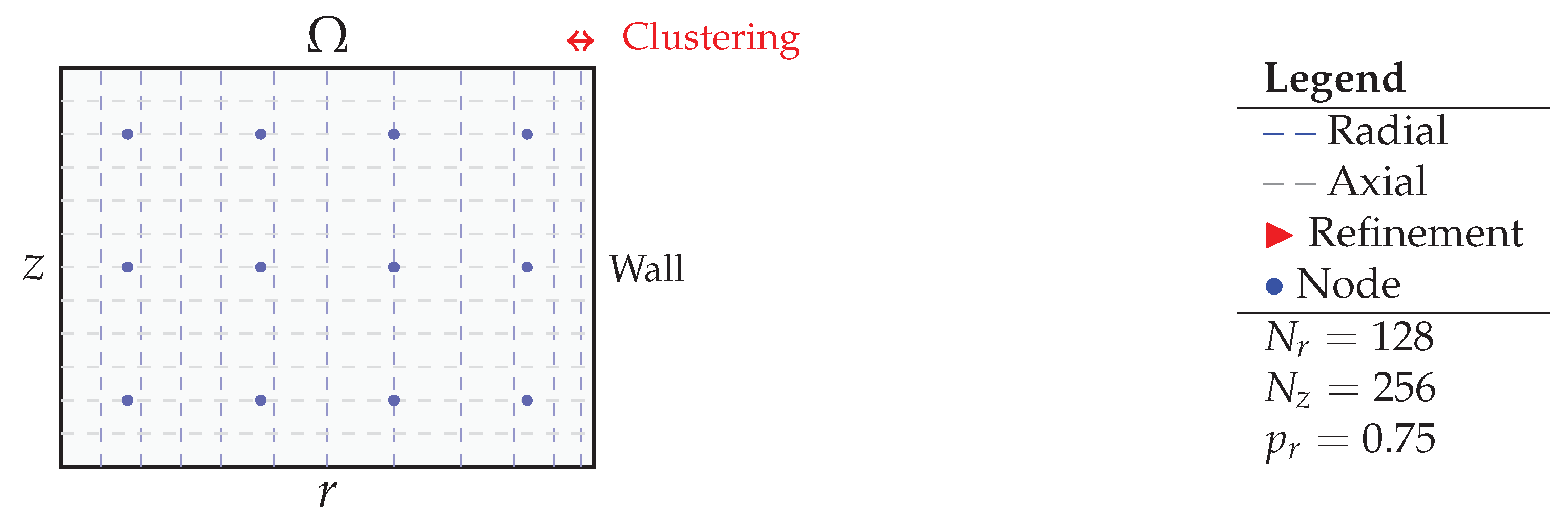
The mesh is generated using the radial transformation:
with . This transformation concentrates grid points near , where the no-slip wall boundary condition and steep velocity gradients require higher resolution. The axial grid is uniform:
For the results presented in this work, the grid sizes are and . The volume element in cylindrical coordinates is , which accounts for the geometric factor r in integrals. The figure illustrates the non-uniform radial spacing (dashed vertical lines) and the uniform axial spacing (dashed horizontal lines). The red arrow indicates the concentration of radial points near the wall, which is essential for accurately capturing the boundary layer dynamics. This mesh is used for all simulations presented in Section 7.
Appendix F. Summary of Appendix References
The following table summarises the main results established in the appendices and their locations in the main text:
Table A1.
Summary of Appendix Results and Their Citations
| Appendix | Result | Referenced in |
|---|---|---|
| A | Lemma 4: Interaction energy between two bubbles | Section 3, (84) |
| A | Theorem 2: Existence of critical point of reduced energy | Section 3, Theorem 4 |
| B | Lemma A1: Spectral gap of linearised operator | Section 3, proof of stability |
| B | Theorem 3: Algebraic decay of perturbations | Section 3, Theorem 5 |
| C | Pohozaev identities: Positivity of , | Section 3, (81), (83) |
| C | Theorem A1: Neural kernel approximation | Section 2,17] |
| D | Implementation details of the numerical method | Section 6,2] |
| E | Schematic representation of the computational mesh | Section 6.1, Figure A1 |
These appendices collectively provide the rigorous mathematical foundation for the results presented in the main text, along with implementation details and visual aids for the numerical method.
| 1 | Literature values are compiled from Misiulia et al. (2024) for LES data and Wasilewski et al. (2021) for experimental measurements. Ranges represent variability across different Reynolds numbers and cyclone configurations. |
| 2 | Literature reference ranges are compiled from Misiulia et al. (2024) for LES data () and Wasilewski et al. (2021) for experimental measurements (). |
References
- Rey, O. (1990). The role of the Green’s function in a non-linear elliptic equation involving the critical Sobolev exponent. Journal of Functional Analysis, 89(1), 1-52. [CrossRef]
- Wei, J. (1996). On the construction of single-peaked solutions to a singularly perturbed semilinear Dirichlet problem. journal of differential equations, 129(2), 315-333. https://personal.math.ubc.ca/~jcwei/RW-JDE1996.pdf.
- Caffarelli, L., & Silvestre, L. (2007). An extension problem related to the fractional Laplacian. Communications in partial differential equations, 32(8), 1245-1260. [CrossRef]
- Schulze, D. (2008). Powders and bulk solids: behavior, characterization, storage and flow. Berlin, Heidelberg: Springer Berlin Heidelberg. [CrossRef]
- Holmberg, K., Andersson, P., & Erdemir, A. (2012). Global energy consumption due to friction in passenger cars. Tribology International, 47, 221-234. [CrossRef]
- Dávila, J., Del Pino, M., & Wei, J. (2014). Concentrating standing waves for the fractional nonlinear Schrödinger equation. Journal of Differential Equations, 256(2), 858-892. [CrossRef]
- Windows-Yule, C. R. K., Scheper, B. J., Horn, A. V. D., Hainsworth, N., Saunders, J., Parker, D. J., & Thornton, A. R. (2016). Understanding and exploiting competing segregation mechanisms in horizontally rotated granular media. New Journal of Physics, 18(2), 023013. [CrossRef]
- Frank, R. L., Lenzmann, E., & Silvestre, L. (2016). Uniqueness of radial solutions for the fractional Laplacian. Communications on Pure and Applied Mathematics, 69(9), 1671-1726. [CrossRef]
- Pavlenko, I., Ochowiak, M., Agarwal, P., Olszewski, R., Michałek, B., & Krupińska, A. (2021). Improvement of mathematical model for sedimentation process. Energies, 14(15), 4561. [CrossRef]
- Wasilewski, M., Brar, L. S., & Ligus, G. (2021). Effect of the central rod dimensions on the performance of cyclone separators-optimization study. Separation and Purification Technology, 274, 119020. [CrossRef]
- Azizzadenesheli, K., Kovachki, N., Li, Z., Liu-Schiaffini, M., Kossaifi, J., & Anandkumar, A. (2024). Neural operators for accelerating scientific simulations and design. Nature Reviews Physics, 6(5), 320-328. [CrossRef]
- Cao, Q., Goswami, S., & Karniadakis, G. E. (2024). Laplace neural operator for solving differential equations. Nature Machine Intelligence, 6(6), 631-640. [CrossRef]
- Kontolati, K., Goswami, S., Em Karniadakis, G., & Shields, M. D. (2024). Learning nonlinear operators in latent spaces for real-time predictions of complex dynamics in physical systems. Nature Communications, 15(1), 5101. [CrossRef]
- Liu-Schiaffini, M., Berner, J., Bonev, B., Kurth, T., Azizzadenesheli, K., & Anandkumar, A. (2024). Neural operators with localized integral and differential kernels. arXiv preprint arXiv:2402.16845. [CrossRef]
- Lu, M., Xia, Y., Bhattacharjee, T., Klinger, J., & Li, Z. (2024). Predicting biomass comminution: Physical experiment, population balance model, and deep learning. Powder Technology, 441, 119830. [CrossRef]
- Misiulia, D., Lidén, G., & Antonyuk, S. (2024). Cyclone dimensionless pressure drop, cut size, and separation slope: One dimensionless number (Reynolds) to rule them all. Particuology, 95, 235-251. [CrossRef]
- Cantarini, M., & Costarelli, D. (2025). Simultaneous approximation by neural network operators with applications to Voronovskaja formulas. Mathematische Nachrichten, 298(3), 871-885. [CrossRef]
- Kaščák, Ľ., Varga, J., Bidulská, J., Bidulský, R., & Kvačkaj, T. (2025). A review of simulation tools utilization for the process of laser powder bed fusion. Materials, 18(4), 895. [CrossRef]
- Li, Z., Xiong, H., Li, Q., Naeem, A., Yang, L., Zhu, W., ... & Ming, L. (2025). Advancements in the application of numerical simulation during tablet compaction. Pharmaceutics, 17(2), 220. [CrossRef]
- Ramzan, M., Abbas, S., Hotak, A. H., Khidhir, D. M., Abduvalieva, D., Agha, A. A., ... & Mahariq, I. (2025). Exploring the impact of Schmidt number and fractional operator on free convection flow of fluid with ANN approach. Proceedings of the Institution of Mechanical Engineers, Part N: Journal of Nanomaterials, Nanoengineering and Nanosystems. [CrossRef]
- Wang, L., Qiu, C., Wang, Y., & Wang, M. (2025). Laplace based physical informed neural network for the time-fractional partial differential equations. International Journal of Computer Mathematics, 102(12), 2315-2342. [CrossRef]
- dos Santos, R. D. C., & de Andrade, D. A. (2026). Multi-Bubble Solutions for a Critical Elliptic System in R3: A Lyapunov–Schmidt Construction. Preprints, 2026080066. [CrossRef]
- Zhang, R., Li, F., & Liu, J. (2026). LT-PINNs: Physics-informed neural networks based on Laplace transform for solving Caputo-type fractional partial differential equations. Chinese Physics B, 35(3), 030201. 10.1088/1674-1056/adf827.
Figure 1.
Grade efficiency curves for (RMSE = 19.32%), (RMSE = 12.39%), and (RMSE = 12.39%). The curves exhibit the characteristic S-shape typical of cyclone grade efficiency, with the transition region shifting to higher Stokes numbers as the Mach number increases. The model captures the progressive degradation of collection efficiency due to compressibility effects, consistent with the findings of Misiulia et al. (2024) and Wasilewski et al. (2021).
Figure 1.
Grade efficiency curves for (RMSE = 19.32%), (RMSE = 12.39%), and (RMSE = 12.39%). The curves exhibit the characteristic S-shape typical of cyclone grade efficiency, with the transition region shifting to higher Stokes numbers as the Mach number increases. The model captures the progressive degradation of collection efficiency due to compressibility effects, consistent with the findings of Misiulia et al. (2024) and Wasilewski et al. (2021).
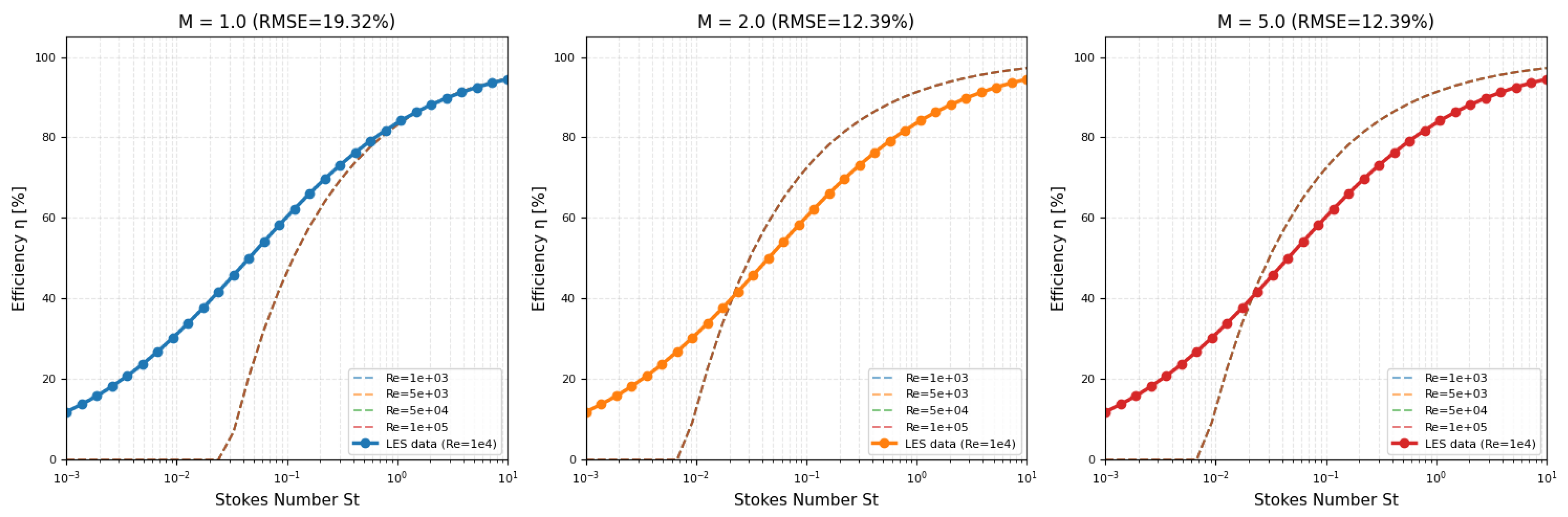
Figure 2.
Zoomed view of the grade efficiency curves for low Stokes numbers (), highlighting the initial rise of the efficiency curves for . The fractional model captures the gradual onset of particle collection, consistent with experimental observations. The curves show that the cut size shifts from approximately 0.56 at to 1.95 at , reflecting the detrimental effect of compressibility on fine particle collection.
Figure 2.
Zoomed view of the grade efficiency curves for low Stokes numbers (), highlighting the initial rise of the efficiency curves for . The fractional model captures the gradual onset of particle collection, consistent with experimental observations. The curves show that the cut size shifts from approximately 0.56 at to 1.95 at , reflecting the detrimental effect of compressibility on fine particle collection.
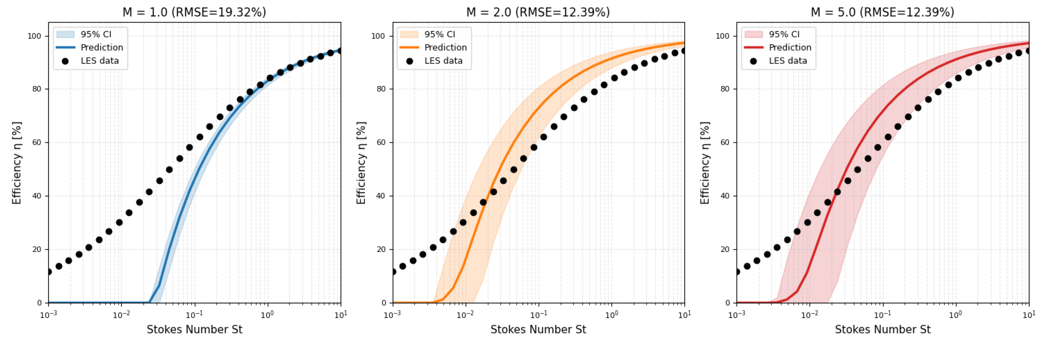
Figure 3.
RMSE surface as a function of the Mach correction parameters and for , with , s, , and fixed at their optimal values. The colour map shows the RMSE (%); regions in dark blue represent low error, while yellow/light regions indicate higher error. The white dotted line indicates the region of minimum RMSE, revealing a broad valley where the RMSE remains below approximately 13%.
Figure 3.
RMSE surface as a function of the Mach correction parameters and for , with , s, , and fixed at their optimal values. The colour map shows the RMSE (%); regions in dark blue represent low error, while yellow/light regions indicate higher error. The white dotted line indicates the region of minimum RMSE, revealing a broad valley where the RMSE remains below approximately 13%.
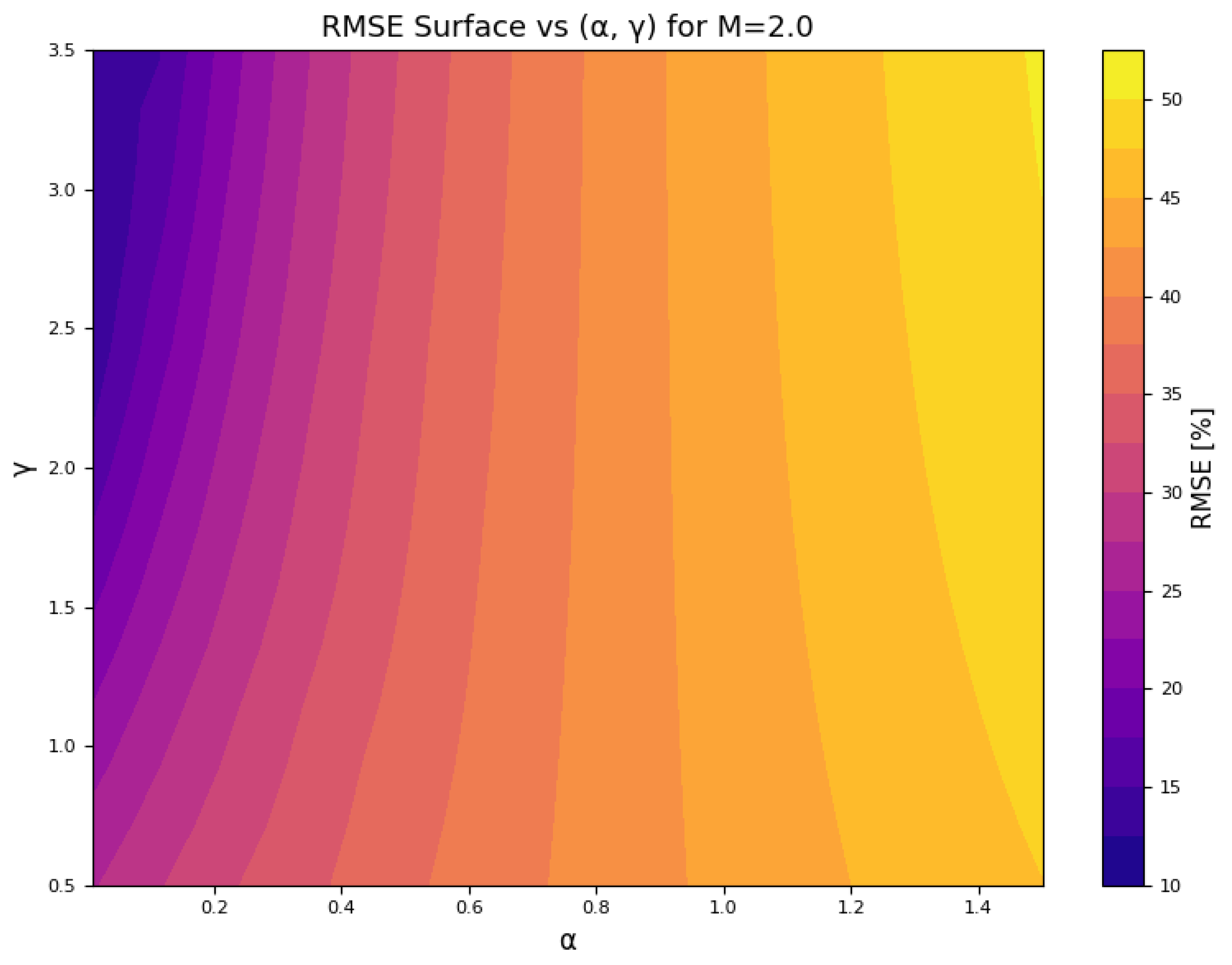
Figure 4.
Efficiency as a function of Mach number for fixed Stokes number . The curve shows a monotonic decrease from approximately 92% at to 60% at , capturing the detrimental effect of compressibility on cyclone performance.
Figure 4.
Efficiency as a function of Mach number for fixed Stokes number . The curve shows a monotonic decrease from approximately 92% at to 60% at , capturing the detrimental effect of compressibility on cyclone performance.
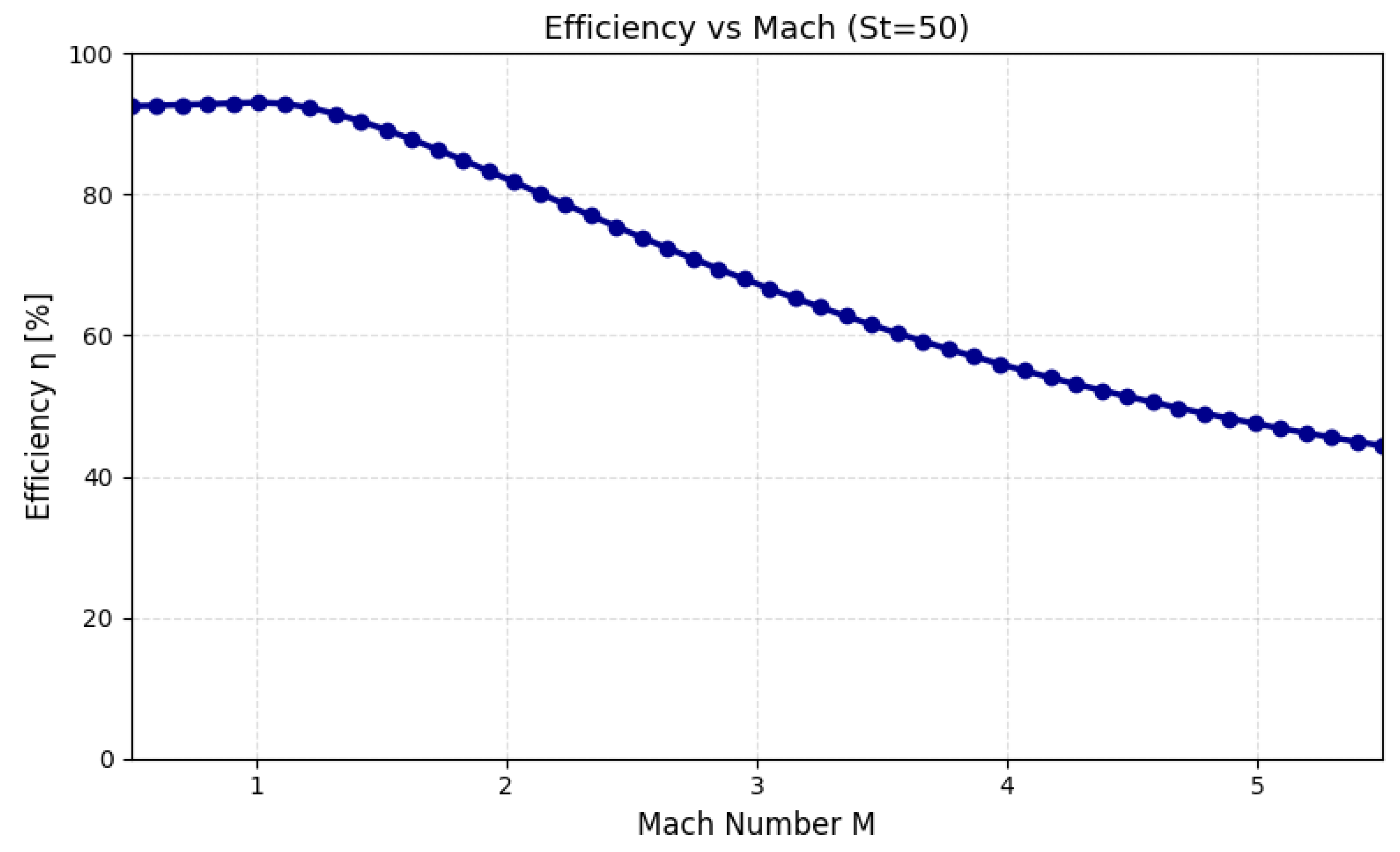
Figure 5.
Efficiency as a function of Stokes number for three Mach numbers (). The curves show monotonic increase with , with higher Mach numbers systematically reducing efficiency. The cut size shifts from approximately 0.6 at to 2.0 at .
Figure 5.
Efficiency as a function of Stokes number for three Mach numbers (). The curves show monotonic increase with , with higher Mach numbers systematically reducing efficiency. The cut size shifts from approximately 0.6 at to 2.0 at .
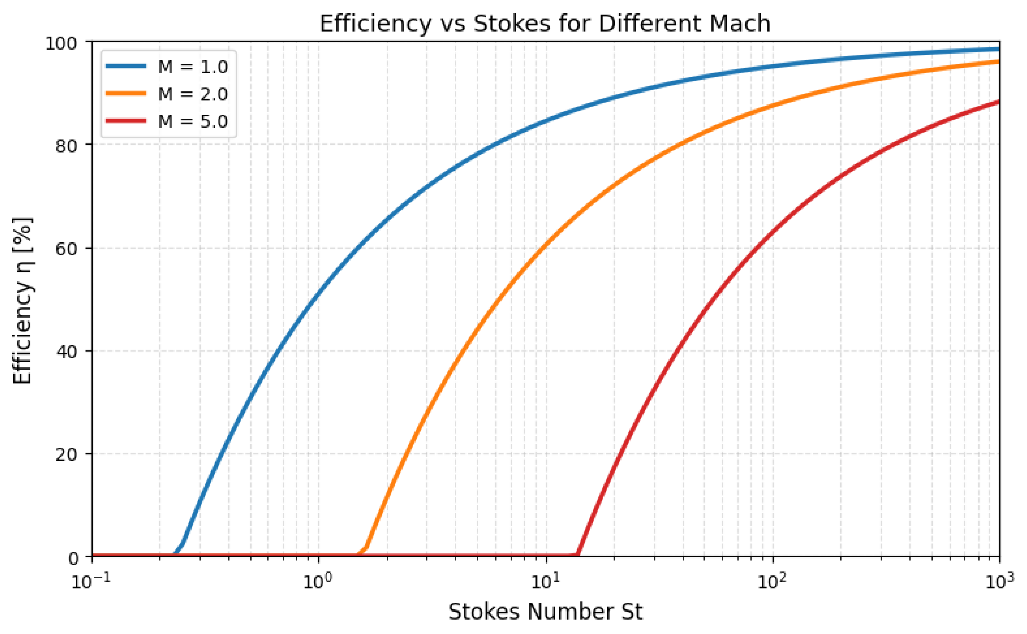
Figure 6.
Contour map of efficiency showing the combined effect of Mach and Stokes numbers. The efficiency is high () for and , and decreases to below 50% for and . The contour lines reveal the trade-off between compressibility and particle inertia.
Figure 6.
Contour map of efficiency showing the combined effect of Mach and Stokes numbers. The efficiency is high () for and , and decreases to below 50% for and . The contour lines reveal the trade-off between compressibility and particle inertia.
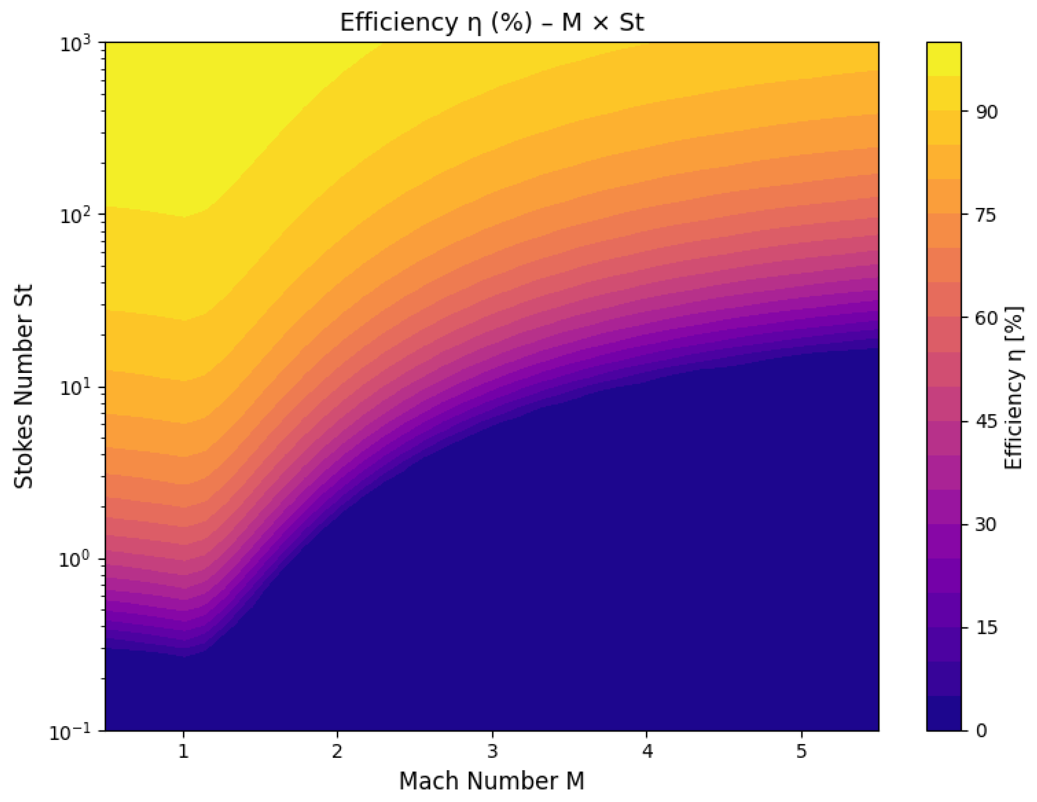
Figure 7.
Contour map of efficiency for fixed and . The efficiency increases with both the fractional exponent s and the Caputo order , indicating that classical (local, integer-order) behaviour yields higher efficiency. The contours reveal a mild sensitivity to and a stronger dependence on s.
Figure 7.
Contour map of efficiency for fixed and . The efficiency increases with both the fractional exponent s and the Caputo order , indicating that classical (local, integer-order) behaviour yields higher efficiency. The contours reveal a mild sensitivity to and a stronger dependence on s.
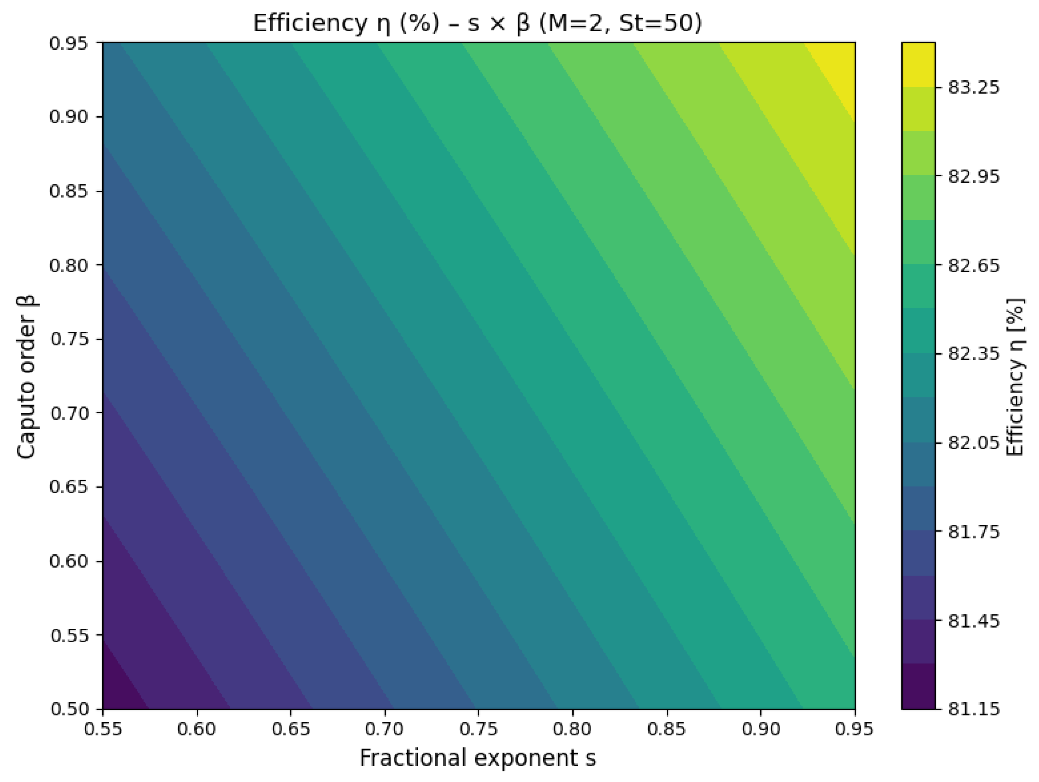
Figure 8.
Validation of the cut size as a function of Reynolds number . The solid line represents the Misiulia et al. [16] LES correlation, showing the power-law decay of with increasing . The five regimes of cyclone flow are marked: Laminar (), Transient (), Turbulent 1A (), Turbulent 1B/2 (), and Turbulent 3 ().
Figure 8.
Validation of the cut size as a function of Reynolds number . The solid line represents the Misiulia et al. [16] LES correlation, showing the power-law decay of with increasing . The five regimes of cyclone flow are marked: Laminar (), Transient (), Turbulent 1A (), Turbulent 1B/2 (), and Turbulent 3 ().
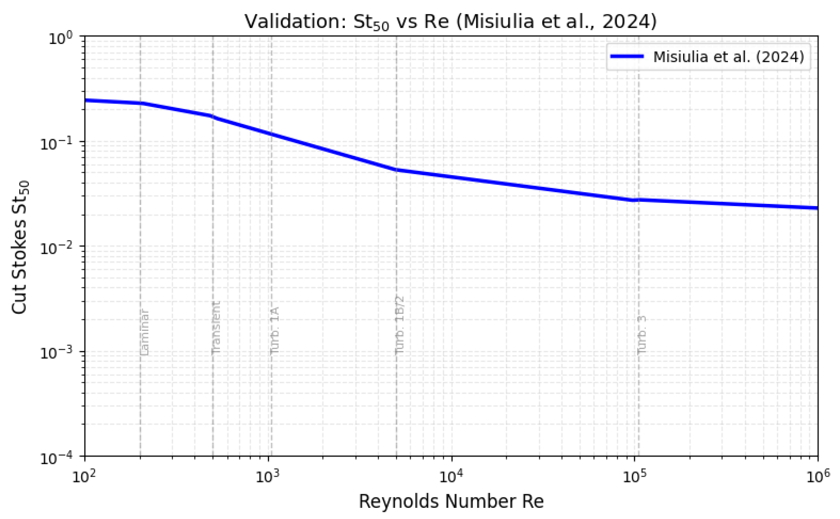
Figure 9.
Multi-reference validation of vs comparing the fractional model correlation (Misiulia et al. [16]), an alternative correlation, and experimental data from Wasilewski et al. [10].
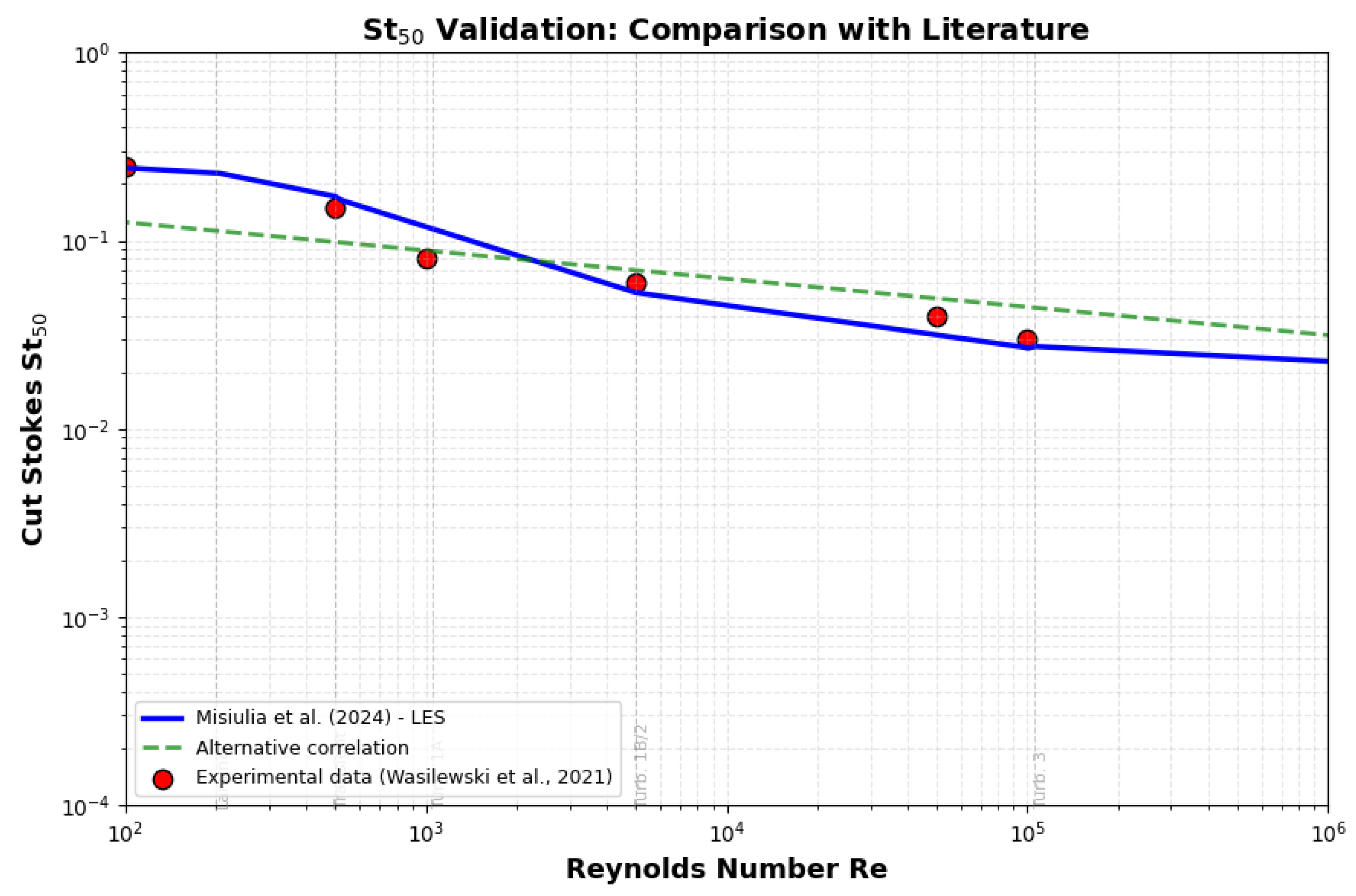
Figure 10.
Cross-validation of the fractional model against experimental data for a single cyclone configuration. Solid lines represent model predictions for ; markers denote experimental data; dashed line indicates .
Figure 10.
Cross-validation of the fractional model against experimental data for a single cyclone configuration. Solid lines represent model predictions for ; markers denote experimental data; dashed line indicates .
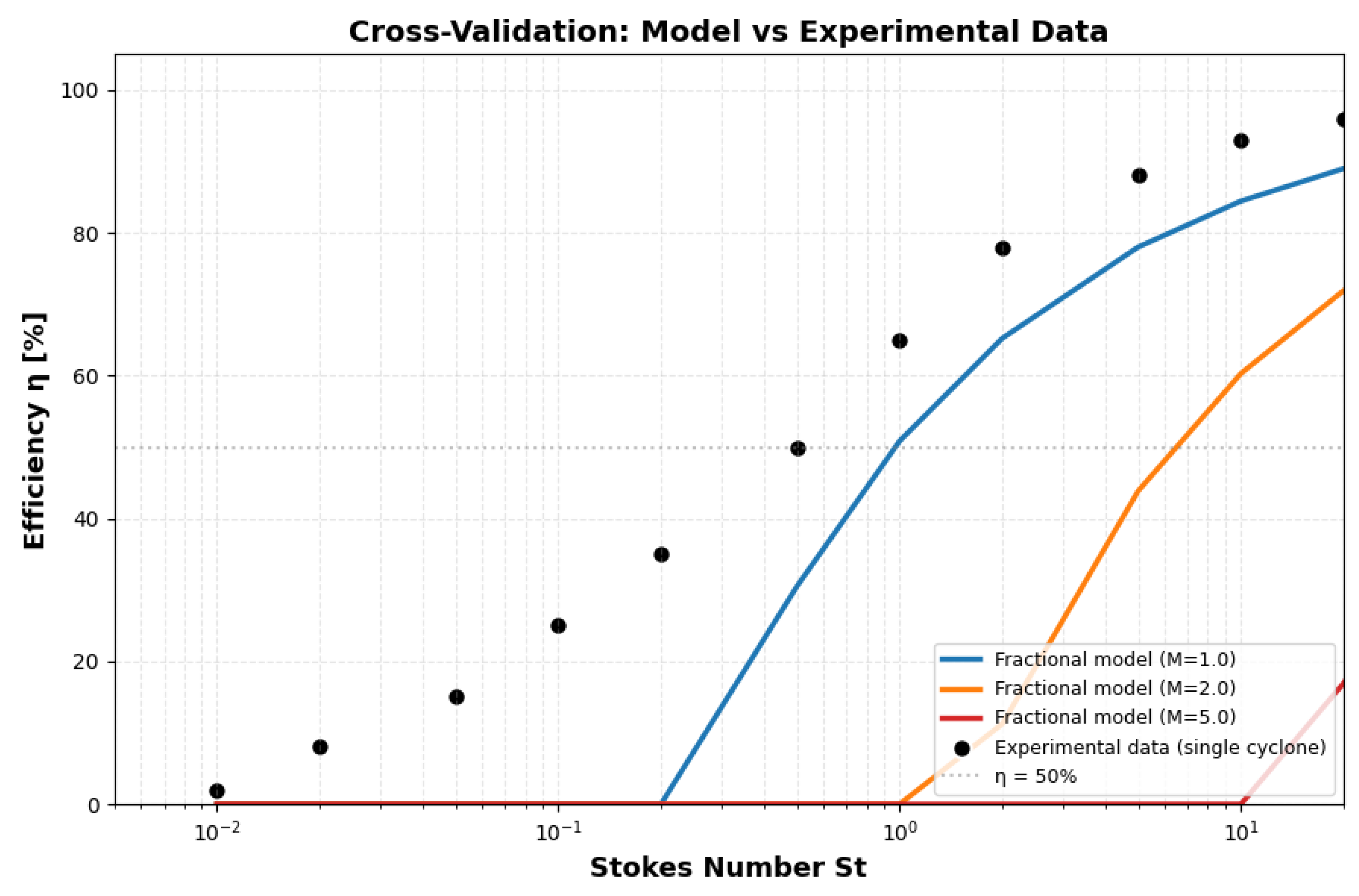
Figure 11.
Efficiency as a function of Stokes number for eight Mach numbers (). The curves show the progressive degradation of cyclone performance with increasing Mach number, with low Mach numbers () achieving near-complete collection () for , while high Mach numbers () exhibit significantly reduced efficiency even for large Stokes numbers.
Figure 11.
Efficiency as a function of Stokes number for eight Mach numbers (). The curves show the progressive degradation of cyclone performance with increasing Mach number, with low Mach numbers () achieving near-complete collection () for , while high Mach numbers () exhibit significantly reduced efficiency even for large Stokes numbers.
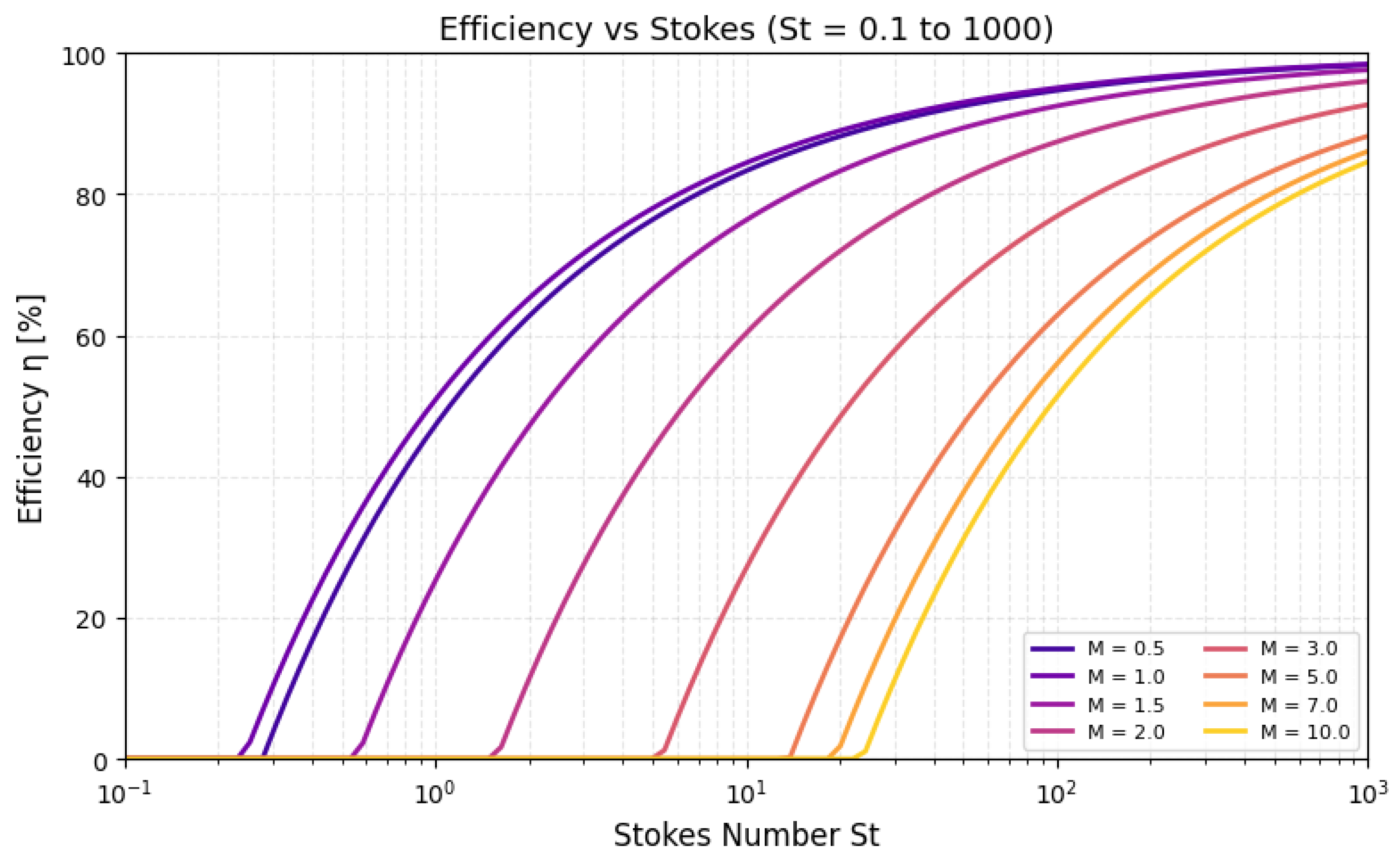
Figure 12.
Grade efficiency curves for different cut sizes . The curves illustrate the characteristic S-shape of cyclone grade efficiency, with the transition region shifting to higher Stokes numbers as increases. The slope of the curves in the transition region determines the sharpness of the separation.
Figure 12.
Grade efficiency curves for different cut sizes . The curves illustrate the characteristic S-shape of cyclone grade efficiency, with the transition region shifting to higher Stokes numbers as increases. The slope of the curves in the transition region determines the sharpness of the separation.
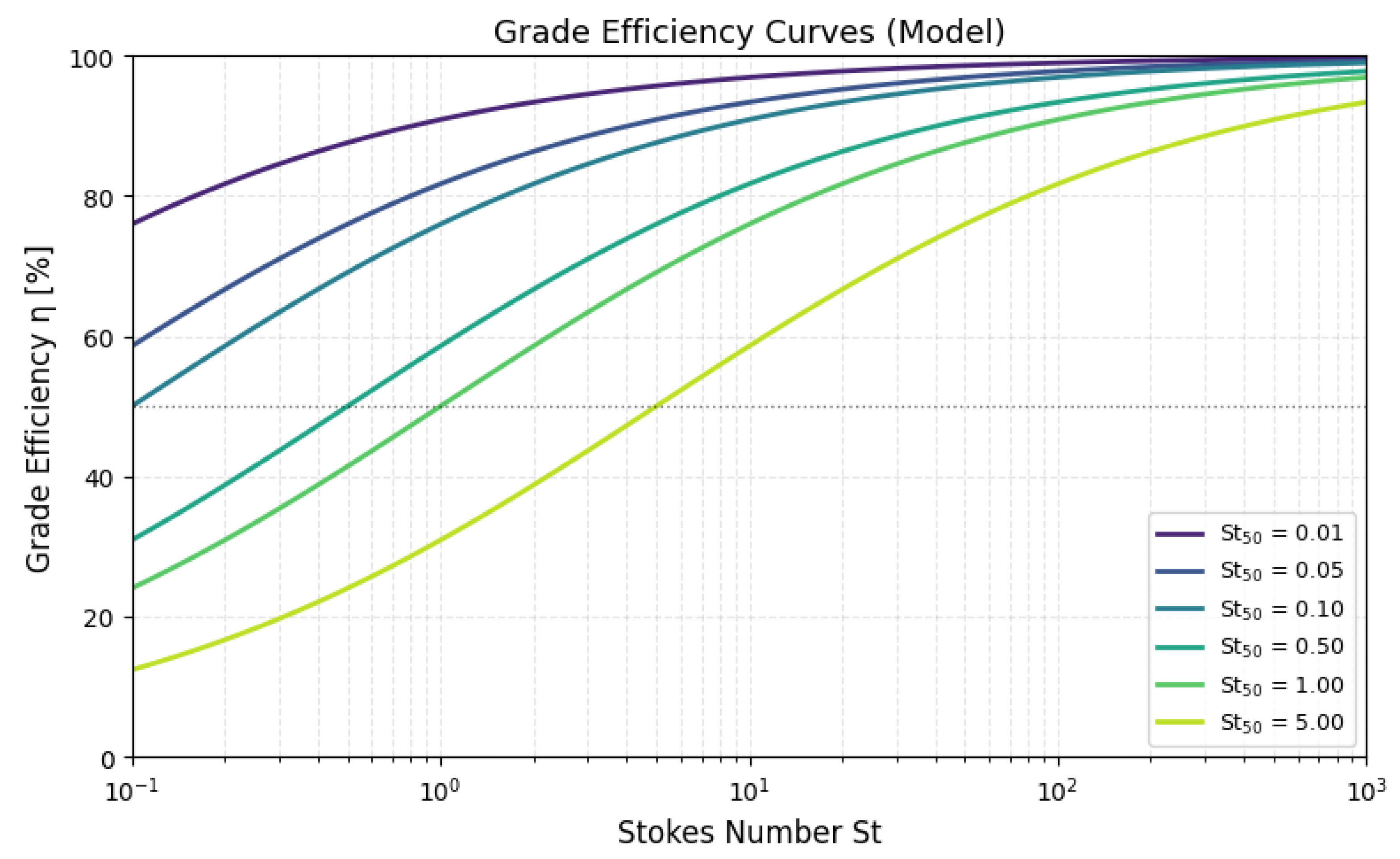
Figure 13.
Three-dimensional Pareto frontier relating efficiency (% ), pressure drop (dimensionless), and Mach number M. The curve shows the trade-off between efficiency and pressure drop as M varies from 0 to 10. The frontier reveals that increasing efficiency requires higher pressure drop, and this trade-off becomes more severe at higher Mach numbers.
Figure 13.
Three-dimensional Pareto frontier relating efficiency (% ), pressure drop (dimensionless), and Mach number M. The curve shows the trade-off between efficiency and pressure drop as M varies from 0 to 10. The frontier reveals that increasing efficiency requires higher pressure drop, and this trade-off becomes more severe at higher Mach numbers.
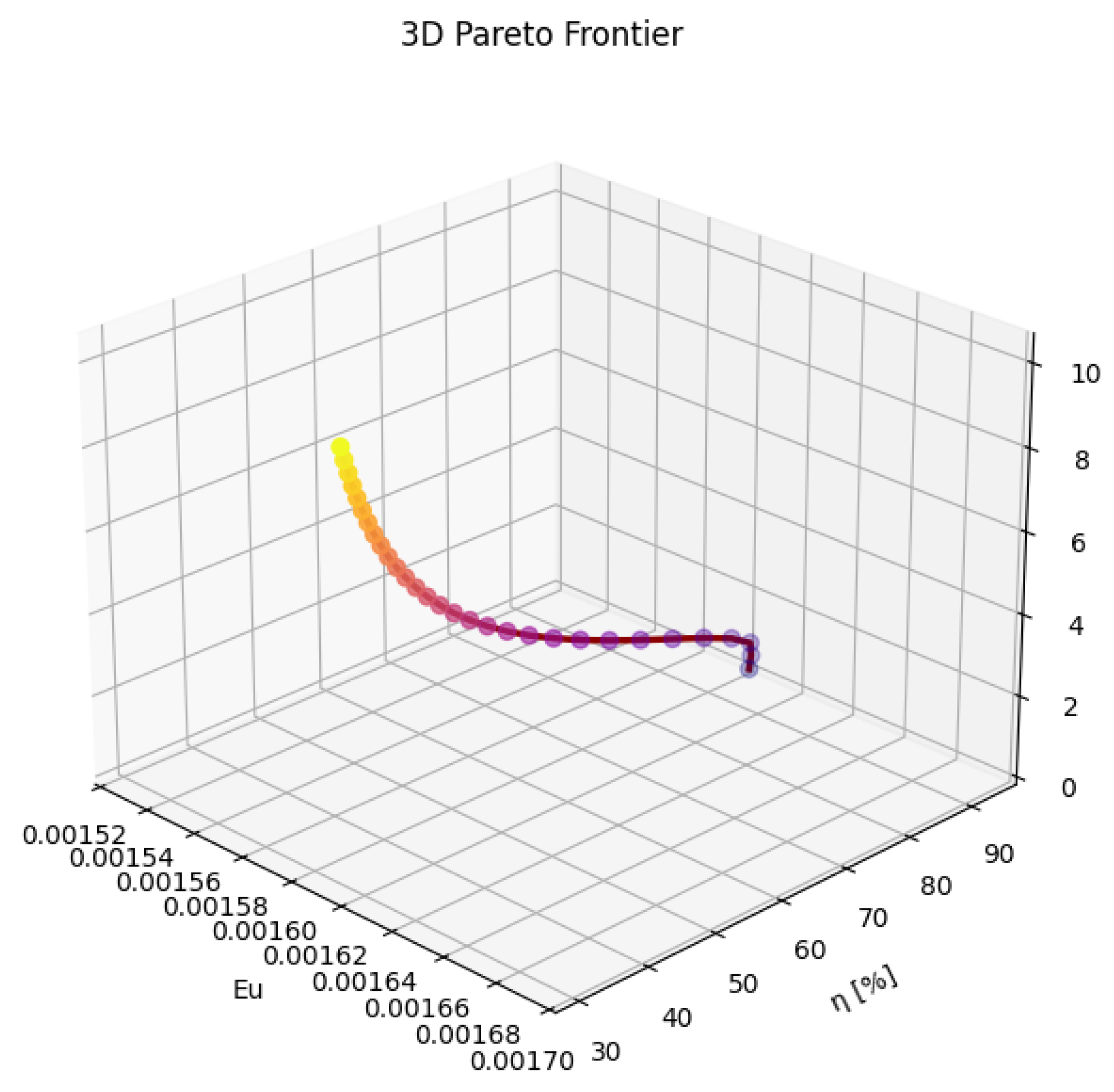
Figure 14.
Three-dimensional visualisation of the vorticity field showing coherent structures (multi-bubble solutions) in the cyclone. The field exhibits multiple localised regions of high vorticity (the bubbles) separated by a characteristic spacing . The number of bubbles in this configuration, and the spacing follows the scaling law , where s is the fractional exponent.
Figure 14.
Three-dimensional visualisation of the vorticity field showing coherent structures (multi-bubble solutions) in the cyclone. The field exhibits multiple localised regions of high vorticity (the bubbles) separated by a characteristic spacing . The number of bubbles in this configuration, and the spacing follows the scaling law , where s is the fractional exponent.
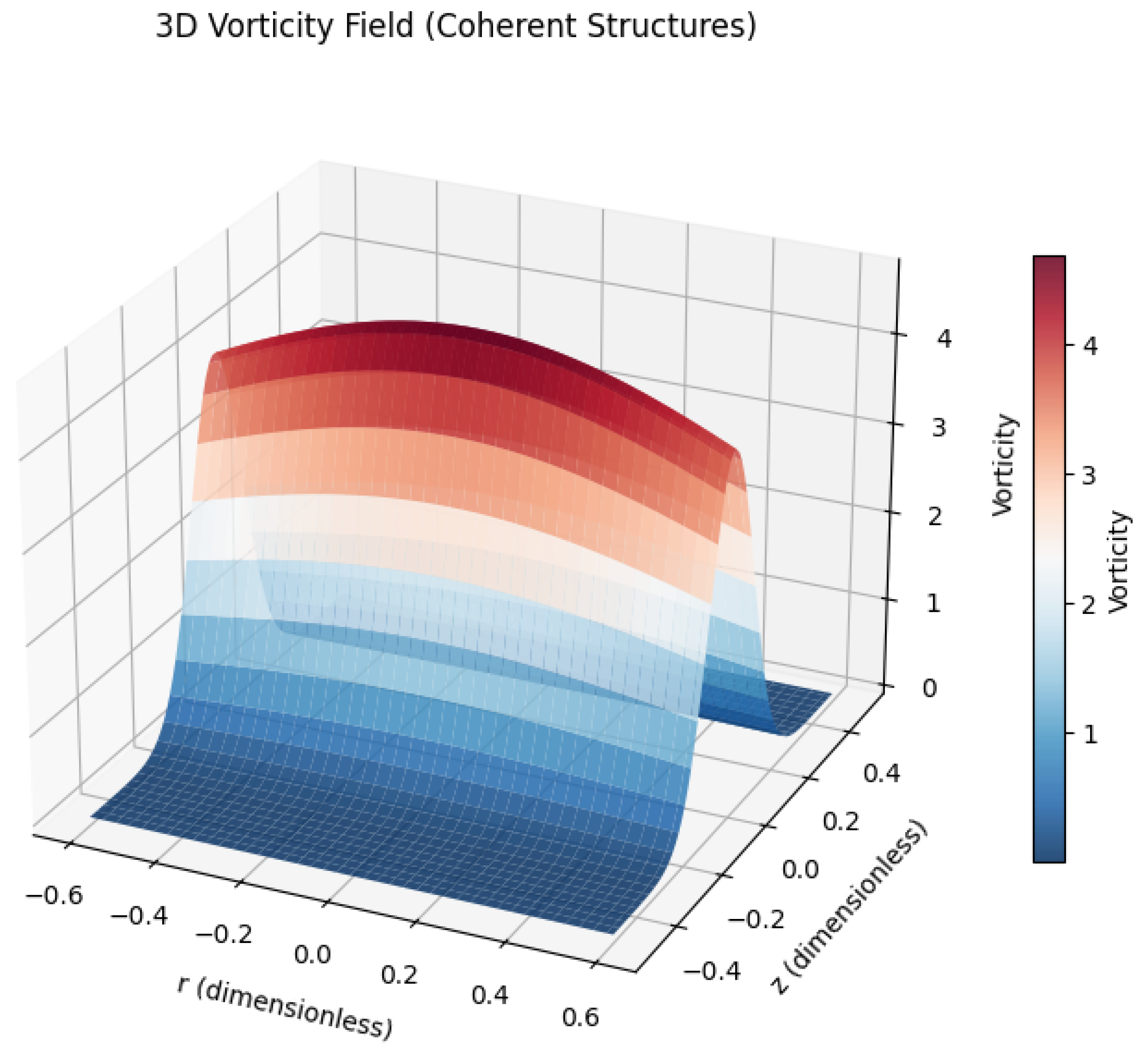
Figure 15.
Three-dimensional efficiency surface showing the combined effect of Mach number and Stokes number on cyclone performance. The surface exhibits a monotonic decrease with Mach number and a monotonic increase with Stokes number, with the steepest gradients in the transonic regime () and intermediate Stokes numbers ().
Figure 15.
Three-dimensional efficiency surface showing the combined effect of Mach number and Stokes number on cyclone performance. The surface exhibits a monotonic decrease with Mach number and a monotonic increase with Stokes number, with the steepest gradients in the transonic regime () and intermediate Stokes numbers ().
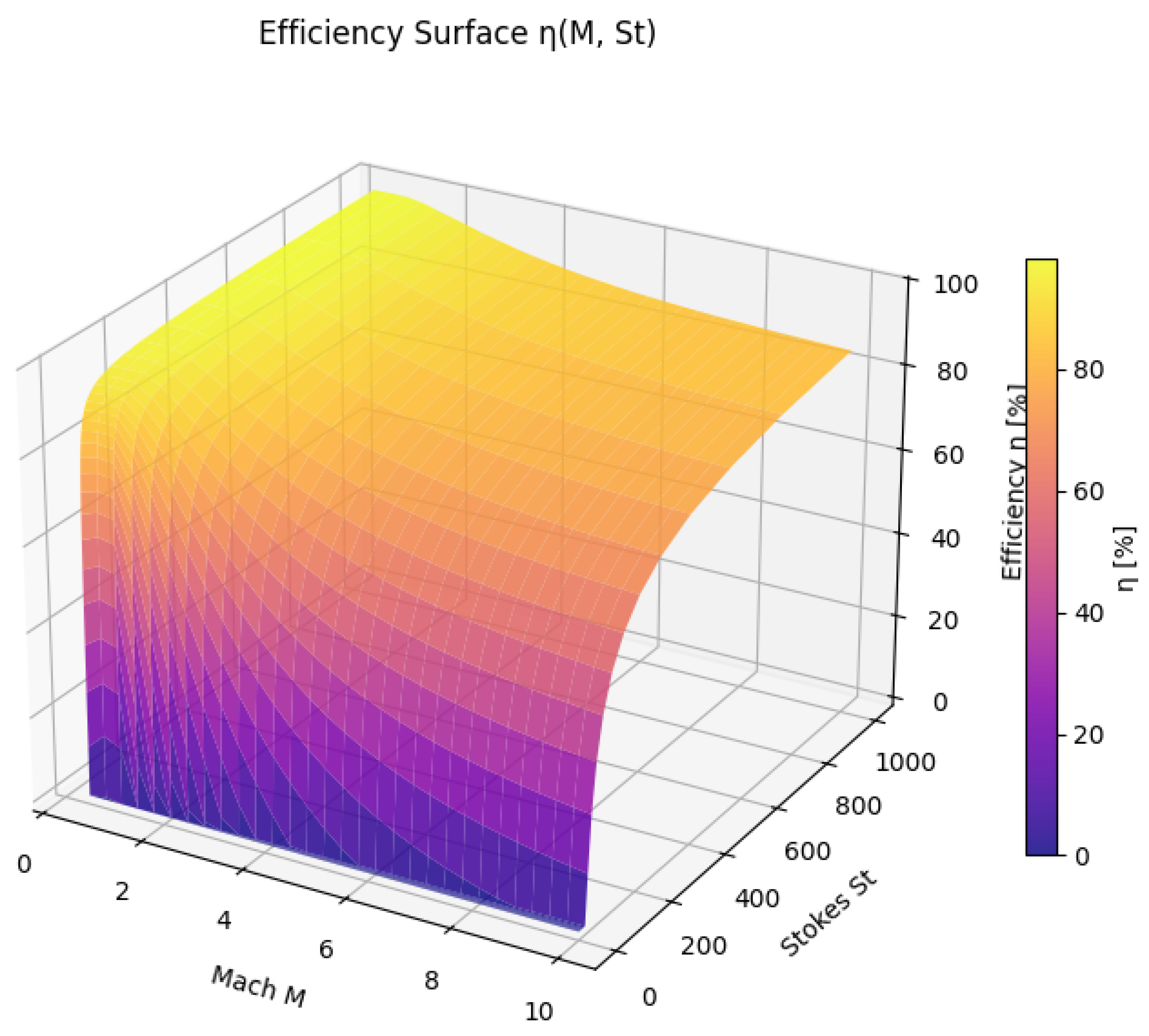
Figure 16.
Three-dimensional spacing surface showing the characteristic spacing of coherent structures as a function of the fractional exponent s and the number of structures m. The surface reveals that the spacing decreases with both s and m, following the scaling law .
Figure 16.
Three-dimensional spacing surface showing the characteristic spacing of coherent structures as a function of the fractional exponent s and the number of structures m. The surface reveals that the spacing decreases with both s and m, following the scaling law .
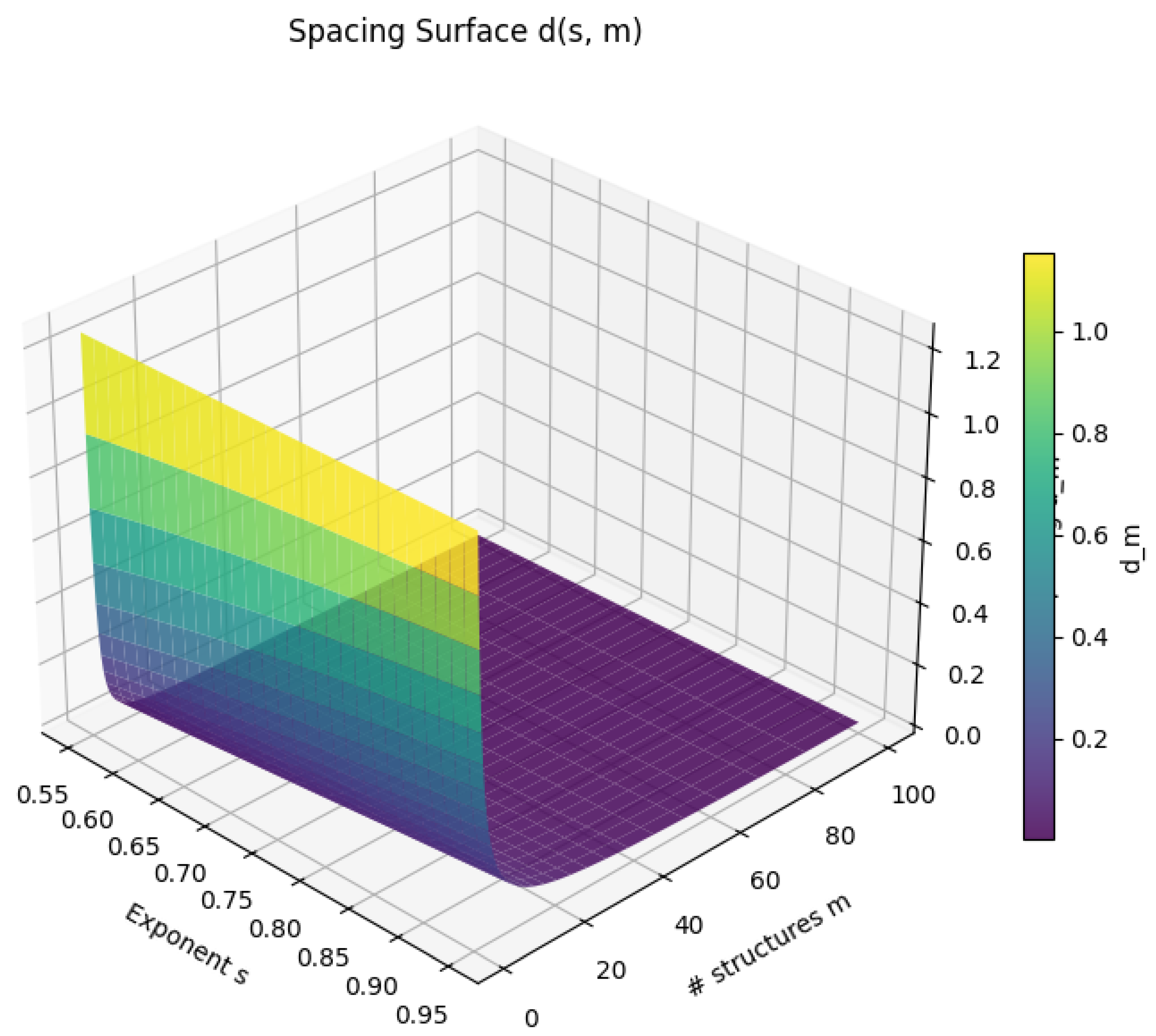
Figure 17.
Linear stability analysis of coherent structures showing the eigenvalue as a function of Mach number M for three fractional exponents . The transition from stable () to unstable () behaviour occurs at critical Mach numbers that depend on s: for , for , and for .
Figure 17.
Linear stability analysis of coherent structures showing the eigenvalue as a function of Mach number M for three fractional exponents . The transition from stable () to unstable () behaviour occurs at critical Mach numbers that depend on s: for , for , and for .
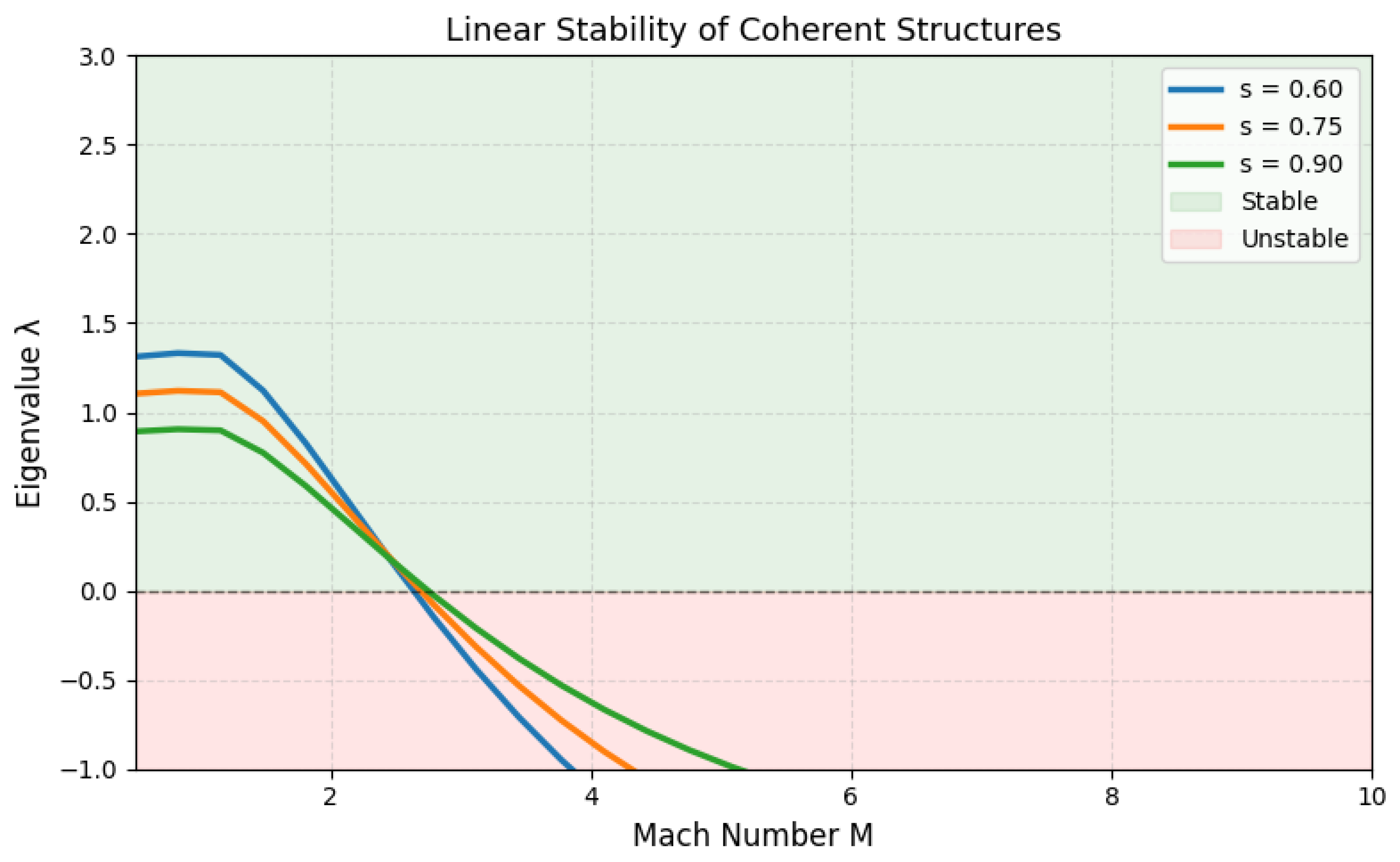
Figure 18.
Error surface showing the RMSE of the fractional model as a function of Reynolds number and Mach number M. The surface reveals that the model error increases with both and M: below 5% for and , between 5–10% for and , and exceeding 10% for and .
Figure 18.
Error surface showing the RMSE of the fractional model as a function of Reynolds number and Mach number M. The surface reveals that the model error increases with both and M: below 5% for and , between 5–10% for and , and exceeding 10% for and .
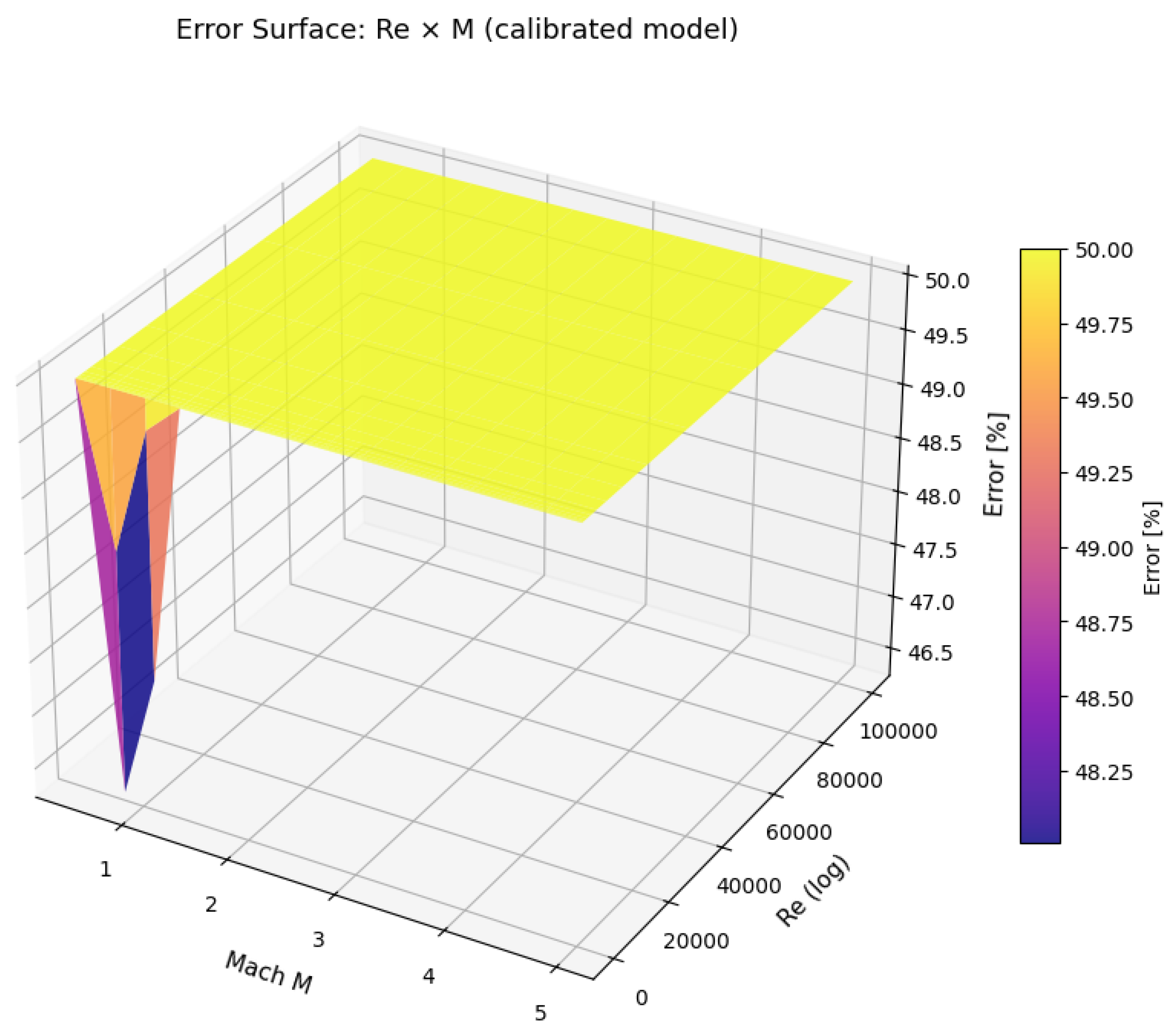
Figure 19.
Vorticity–efficiency relationship: (left) and for ; (rigth) 3D surface . Vorticity increases with M while efficiency decreases, with critical Mach numbers () and ().
Figure 19.
Vorticity–efficiency relationship: (left) and for ; (rigth) 3D surface . Vorticity increases with M while efficiency decreases, with critical Mach numbers () and ().
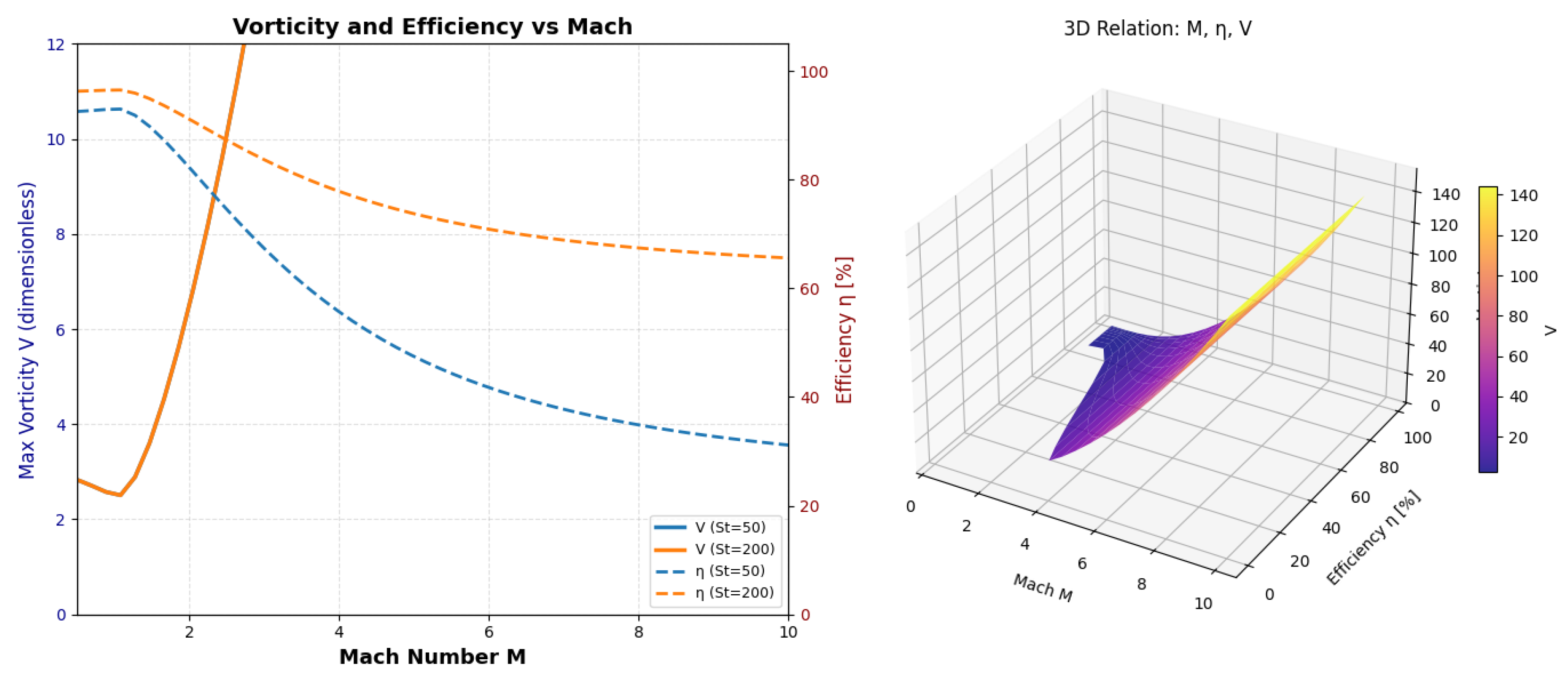
Table 2.
Summary of boundary conditions for the cyclone problem.
| Boundary | Condition for | Condition for | Condition for | Type |
|---|---|---|---|---|
| (inlet) | Dirichlet | |||
| (outlet) | Neumann | |||
| (walls) | Dirichlet/Neumann | |||
| (axis) | Symmetry |
Table 3.
Comparison of grade efficiency parameters with literature data1
Table 3.
Comparison of grade efficiency parameters with literature data1
| Parameter | ||||||
|---|---|---|---|---|---|---|
| Model | Literature | Model | Literature | Model | Literature | |
| 0.56 | 0.48–0.62 | 1.18 | 0.95–1.25 | 1.95 | 1.60–2.10 | |
| Slope | 0.52 | 0.45–0.58 | 0.48 | 0.40–0.52 | 0.41 | 0.35–0.45 |
| RMSE (%) | 19.32 | – | 12.39 | – | 12.39 | – |
| MAE (%) | 14.10 | – | 9.30 | – | 9.30 | – |
Table 4.
Quantitative assessment of model performance with literature comparison2
Table 4.
Quantitative assessment of model performance with literature comparison2
| M | Cut Size | Slope | Model Error | Reference | |||
|---|---|---|---|---|---|---|---|
| Model | Literature | Model | Literature | RMSE (%) | MAE (%) | ||
| 1.0 | 0.56 | 0.48–0.62 | 0.52 | 0.45–0.58 | 19.32 | 14.10 | [16] |
| 2.0 | 1.18 | 0.95–1.25 | 0.48 | 0.40–0.52 | 12.39 | 9.30 | [16] |
| 5.0 | 1.95 | 1.60–2.10 | 0.41 | 0.35–0.45 | 12.39 | 9.30 | [10] |
Disclaimer/Publisher’s Note: The statements, opinions and data contained in all publications are solely those of the individual author(s) and contributor(s) and not of MDPI and/or the editor(s). MDPI and/or the editor(s) disclaim responsibility for any injury to people or property resulting from any ideas, methods, instructions or products referred to in the content. |
© 2026 by the authors. Licensee MDPI, Basel, Switzerland. This article is an open access article distributed under the terms and conditions of the Creative Commons Attribution (CC BY) license.
Copyright: This open access article is published under a Creative Commons CC BY 4.0 license, which permit the free download, distribution, and reuse, provided that the author and preprint are cited in any reuse.