A Local Fixed Point Theorem for Multivalued Mappings in Strong Partial b-Metric Spaces with Potential Applications to Language Dynamics

1. Introduction

Fixed point theory provides one of the fundamental mathematical tools for analyzing the existence and stability of equilibrium states, iterative algorithms, optimization procedures, and learning processes. In many applications, however, the underlying dynamics are meaningful only in a prescribed neighborhood of an initial state, while global contractive assumptions are either unavailable or unnecessarily restrictive. This has led to the development of local fixed point principles, where the iteration is required to remain inside a suitable ball and converge to a fixed point without relying on global properties of the entire space.

The study of generalized metric structures has substantially enlarged the scope of classical fixed point theory. Besides ordinary metric spaces, numerous extensions have been introduced in order to model situations in which the standard notion of distance is no longer appropriate. Among the best known are partial metric spaces, introduced by Matthews, b-metric spaces, strong b-metric spaces, partial b-metric spaces, and strong partial metric spaces. The class of strong partial b-metric spaces forms an intermediate class between strong b-metric spaces and partial b-metric spaces. It combines the possibility of positive self-distances with the asymmetric coefficient K appearing in the strong generalized triangle inequality. Partial metric spaces are recovered when $K=1$, while ordinary metric spaces are recovered when, in addition, all self-distances vanish.

The position of strong partial b-metric spaces between strong b-metric spaces and partial b-metric spaces was established by Moshokoa and Ncongwane; see [1].

Unlike classical metric spaces, positive self-distances may carry meaningful information rather than merely representing a technical generalization. In many situations, they naturally quantify the amount of incompleteness, uncertainty, or residual discrepancy associated with a given state. Consequently, a point with a positive self-distance should not necessarily be interpreted as being “far from itself,” but rather as representing an object that has not yet reached its final stable form. This interpretation makes strong partial b-metric spaces particularly suitable for describing progressive refinement processes.

A subtle issue in partial b-metric spaces concerns the topological behavior of their open balls. Ge and Lin showed that, in general, the family of partial b-metric open balls need not form a basis for a topology; see [2]. Since strong partial b-metric spaces constitute a more restrictive class, such a topological failure should not be transferred to the present setting without additional justification. Accordingly, our arguments do not require the family of p-balls to form a topological basis: the closed ball is used only as a localization set for the iterative construction. Moreover, because the iterative sequence constructed below is 0-Cauchy, 0-completeness is the natural completeness assumption for the fixed point argument developed here.

The purpose of the present paper is to establish a local fixed point principle for multivalued mappings acting on 0-complete strong partial b-metric spaces. The contraction condition is formulated by means of Bianchini–Grandolfi gauge functions and is expressed through a set-valued excess generated by the strong partial b-metric. This approach simultaneously combines localization, multivalued mappings, nonlinear contractions, and generalized metric structures within a single framework.

A closely related local multivalued fixed point framework was obtained by Slimani, Graef, and Ouahab [3] for complete strong b-metric spaces. Their local results employ a one-sided set excess on a closed ball together with linear contractive conditions. The present setting differs in several essential respects: the underlying space is a 0-complete strong partial b-metric space, positive self-distances are allowed, the values of the multifunction are treated through 0-closedness, and the linear contraction modulus is replaced by a Bianchini–Grandolfi gauge. The localization argument must therefore be adapted to the strong partial b-metric inequality and to the corresponding notion of 0-convergence.

The obtained theorem yields, as immediate consequences, local versions of several familiar contractive principles, including the linear contraction case. The proof is based on an explicit construction of an iterative sequence inside a prescribed ball together with chain estimates adapted to the asymmetric role of the coefficient K in the strong partial b-metric inequality. The argument explicitly accommodates positive self-distances and uses the corresponding notion of 0-completeness in order to obtain the required limiting behavior.

Although the present paper is purely theoretical, the proposed framework admits natural interpretations in learning and refinement processes. One motivating example comes from mathematical models of linguistic enrichment. In such models, a text is regarded as a state of an iterative editing process rather than as a static object. The positive self-distance of a formulation may then be interpreted as a quantitative measure of its remaining discrepancy from a prescribed stable target family, while a multivalued mapping associates with each text the family of all acceptable subsequent revisions. The multivalued character of the model allows several admissible revisions of the same formulation and may also permit more than one stable formulation, without requiring every possible revision path to converge.

To illustrate this interpretation, the final section presents an abstract enrichment model together with a linguistic realization in which the successive states correspond to increasingly refined versions of the same mathematical statement. Within this model, the self-distance is generated by the transformed shortest distance from the current state to the prescribed stable target family, thereby providing an intrinsic geometric interpretation of positive self-distances in strong partial b-metric spaces.

A recently proposed linguistic enrichment framework interprets language development not merely as the accumulation of new lexical and grammatical resources, but as a broader process involving correction, selection, replacement, adaptation, and stylistic refinement [4]. This interpretation is consistent with usage-based and complex dynamic approaches, according to which linguistic systems are continuously reorganized through interaction, experience, and changing communicative conditions [5,6].

Within this framework, linguistic smoothing refers to the correction of grammatical, lexical, terminological, and stylistic deficiencies, whereas enrichment includes the acquisition and functional differentiation of expressions appropriate to particular discourse contexts. Repeated smoothing and enrichment operations may lead to several stable linguistic outcomes rather than to a unique final text [4]. The present paper develops a complementary metric interpretation of this process. Linguistic states are organized into successive refinement levels, their mutual separation is measured by a revision metric, and their self-distances quantify the remaining effort required to reach the family of stable formulations.

2. Materials and Methods

Throughout the paper, ${\mathbb{R}}_{+}=[0,\infty )$, and all sets under consideration are assumed to be nonempty unless stated otherwise.

This section introduces the generalized metric framework and the auxiliary results required for the proof of the main theorem. Since the local fixed point principle established in this paper is formulated in the setting of strong partial b-metric spaces, we begin with the definition of this class and explain its relation to several classical metric-type structures. We then discuss a number of elementary properties that will play a fundamental role in the construction of the local iterative process and in the subsequent chain estimates.

2.1. Strong Partial b-Metric Spaces

Definition 1.

([1]) Let X be a nonempty set and let $K\ge 1$. A mapping $p:X\times X⟶{\mathbb{R}}_{+}$ is called a strong partial b-metric if, for every $x,y,z\in X$, the following conditions are satisfied:

I 

$x=y$, provided that $p(x,x)=p(x,y)=p(y,y)$;

II 

$p(x,x)\le p(x,y)$;

III 

$p(x,y)=p(y,x)$;

IV 

$p(x,y)\le p(x,z)+Kp(z,y)-p(z,z)$.

The triple $(X,p,K)$ is called a strong partial b-metric space.

The parameter K measures the deviation from the classical triangle inequality, whereas positive self-distances distinguish strong partial b-metrics from ordinary metric-type structures. As will become clear in the subsequent sections, both features are explicitly accommodated by the local fixed point framework developed in this paper.

Remark 1.

The definition of a strong partial b-metric is closely related to several well-known generalized metric structures. Some of them are obtained by imposing additional restrictions on the above definition, whereas partial b-metrics arise after replacing the strong triangle inequality by the corresponding weaker b-metric-type inequality.

1.

If $p(x,x)=0$ for any $x\in X$, then condition (d) becomes $p(x,y)\le p(x,z)+Kp(z,y)$, and $(X,p,K)$ is a strong b-metric space.

2.

If, in addition, $K=1$, then $p(x,y)\le p(x,z)+p(z,y)$, so p is an ordinary metric.

3.

If $K=1$, then condition (d) becomes the usual partial metric triangle inequality, and one recovers the class of partial metric spaces.

4.

Replacing (d) by $p(x,y)\le K\left(p(x,z)+p(z,y)\right)-p(z,z)$ yields the partial b-metric introduced by Shukla [7].

5.

Finally, choosing $K=1$ in the previous inequality gives the classical partial metric introduced by Matthews [8].

Hence, strong partial b-metric spaces should be viewed as an intermediate class between strong b-metric spaces and partial b-metric spaces. In particular, imposing $p(x,x)=0$ yields a strong b-metric, while setting $K=1$ yields a partial metric. Imposing both conditions recovers the ordinary metric case. On the other hand, every strong partial b-metric satisfies the corresponding partial b-metric inequality, but a general partial b-metric need not satisfy the stronger inequality required of a strong partial b-metric. From this point onward, all results are formulated in the setting of strong partial b-metric spaces. Consequently, they immediately specialize to strong b-metric spaces, partial metric spaces, and ordinary metric spaces under the corresponding additional assumptions. They should not, however, be regarded as automatic results for arbitrary partial b-metric spaces.

Although condition (d) appears asymmetric because the coefficient K is attached only to one of the two terms involving the intermediate point, this asymmetry is only apparent. Owing to the symmetry of the distance function, the coefficient may equivalently be placed before either summand. This simple observation will be useful later in the derivation of the chain estimates.

Proposition 1.

Let X be a nonempty set, let $K\ge 1$, and let $p:X\times X⟶{\mathbb{R}}_{+}$ be symmetric. Then the following two inequalities are equivalent:

$$p(x,y)\le p(x,z)+Kp(z,y)-p(z,z),$$

(1)

and

$$p(x,y)\le Kp(x,z)+p(z,y)-p(z,z),$$

(2)

for all $x,y,z\in X$.

Proof. 

Assume first that (1) holds. Let $x,y,z\in X$. Applying (1) to the ordered triple $(y,x,z)$, we obtain $p(y,x)\le p(y,z)+Kp(z,x)-p(z,z)$. By the symmetry of p, we have $p(y,x)=p(x,y)$, $p(y,z)=p(z,y)$, and $p(z,x)=p(x,z)$.

Therefore, $p(x,y)\le p(z,y)+Kp(x,z)-p(z,z)$, which is precisely $p(x,y)\le Kp(x,z)+p(z,y)-p(z,z)$.

Hence (2) holds.

Conversely, suppose that (2) holds. Applying it to the ordered triple $(y,x,z)$, we obtain

$$p(y,x)\le Kp(y,z)+p(z,x)-p(z,z).$$

Using again the symmetry of p, it follows that $p(x,y)\le Kp(z,y)+p(x,z)-p(z,z)$ or equivalently, $p(x,y)\le p(x,z)+Kp(z,y)-p(z,z)$.

Thus (1) holds, and the two inequalities are equivalent. □

Remark 2.

Proposition 1 shows that the apparent asymmetry in the strong partial b-metric inequality is only formal. Although the coefficient K is placed before one of the two terms, the symmetry of p allows the inequality to be used in either orientation.

This observation may lead to two different estimates when the inequality is applied repeatedly along a finite chain $x_0,x_1,\dots ,x_n$. Depending on the chosen orientation, the powers of K may accumulate from the beginning or from the end of the chain. Consequently, both estimates are valid, and in applications one may use the sharper of the two.

Proposition 2.

Let X be a nonempty set, let $K\ge 1$, and let $p:X\times X⟶{\mathbb{R}}_{+}$ satisfy the symmetry condition $p(x,y)=p(y,x)$ for all $x,y\in X$. Then the strong partial b-metric inequality

$$p(x,y)\le p(x,z)+Kp(z,y)-p(z,z)$$

(3)

holds for all $x,y,z\in X$ if and only if

$$p(x,y)\le min\left\{p(x,z)+Kp(z,y),Kp(x,z)+p(z,y)\right\}-p(z,z)$$

(4)

holds for all $x,y,z\in X$.

Moreover, if $p(x,x)=0$ for all $x\in X$, then the same conclusion holds for strong b-metrics, i.e, $p(x,y)\le p(x,z)+Kp(z,y)$ is equivalent to

$$p(x,y)\le min\left\{p(x,z)+Kp(z,y),Kp(x,z)+p(z,y)\right\}.$$

Remark 3.

Consequently, condition (d) in the definition of a strong partial b-metric may equivalently be replaced by (4).

Proof. 

Assume first that (3) holds. Applying this inequality to the ordered triple $(y,x,z)$, we obtain $p(y,x)\le p(y,z)+Kp(z,x)-p(z,z)$.

Using the symmetry of p, it follows that $p(x,y)\le Kp(x,z)+p(z,y)-p(z,z)$.

Therefore, $p(x,y)$ is bounded above by both

$$p(x,z)+Kp(z,y)-p(z,z)$$

and

$$Kp(x,z)+p(z,y)-p(z,z).$$

Hence $p(x,y)\le min\left\{p(x,z)+Kp(z,y),Kp(x,z)+p(z,y)\right\}-p(z,z)$.

Conversely, suppose that (4) holds. Since

$$min\left\{p(x,z)+Kp(z,y),Kp(x,z)+p(z,y)\right\}\le p(x,z)+Kp(z,y),$$

we obtain $p(x,y)\le p(x,z)+Kp(z,y)-p(z,z)$. Thus (3) holds.

Finally, if $p(x,x)=0$ for every $x\in X$, then in particular $p(z,z)=0$. Therefore, the strong partial b-metric inequalities reduce respectively to $p(x,y)\le p(x,z)+Kp(z,y)$ and

$$p(x,y)\le min\left\{p(x,z)+Kp(z,y),Kp(x,z)+p(z,y)\right\}.$$

This proves the corresponding equivalence for strong b-metrics. □

Remark 4.

The minimum formulation is therefore valid both in strong partial b-metric spaces and in strong b-metric spaces. In the latter case, the self-distance correction term disappears, while the symmetry argument remains unchanged.

The previous definition is closely related to several well-established generalized metric structures. The following examples, taken from the literature, illustrate these spaces and emphasize the progressive transition from ordinary metrics to strong partial b-metrics. These examples will be revisited in the subsequent subsections in order to compare the corresponding balls, point-to-set distances, and excesses.

Example 1.

[Classical examples] The following examples illustrate the generalized metric structures discussed above.

1.

Metric space: Let $X=\mathbb{R}$ and define $d(x,y)=|x-y|$. Then $(\mathbb{R},d)$ is a metric space.

2.

b-metric space: Let $X=\mathbb{R}$ and let $d(x,y)={|x-y|}^2$. Then $d(x,z)\le 2\left(d\right(x,y)+d(y,z\left)\right)$, so $(\mathbb{R},d,2)$ is a b-metric space in the sense of Czerwik [9]. It is not a metric space since the ordinary triangle inequality fails.

3.

Strong b-metric space: Let $X=\mathbb{R}$, define $h\left(t\right)=t+{\displaystyle \frac{t^2}{1+t}}$ for $t\ge 0$, and put $d(x,y)=h\left(\right|x-y\left|\right)$. Since h is increasing and $h^{\prime }\left(t\right)=2-{\displaystyle \frac{1}{{(1+t)}^2}}\le 2,$ the mean value theorem gives $h(a+b)-h\left(a\right)\le 2b\le 2h\left(b\right)$ for all $a,b\ge 0$. Consequently, $d(x,z)\le d(x,y)+2d(y,z),$ so $(\mathbb{R},d,2)$ is a strong b-metric space. It is not a metric space, since

$$d(0,2)=h\left(2\right)={\displaystyle \frac{10}{3}}>3=2h\left(1\right)=d(0,1)+d(1,2).$$

4.

Partial metric space: Let $X={\mathbb{R}}_{+}$ and define $p(x,y)=\max \{x,y\}$. Then p is the classical partial metric introduced by Matthews [8]. Here $p(x,x)=x$. so every point possesses a positive self-distance.

5.

Partial b-metric space: Let $X={\mathbb{R}}_{+}$ and define $p(x,y)={\left(\max \{x,y\}\right)}^2$. This is one of the standard examples of a partial b-metric given by Shukla [7]. The self-distances are positive, and the generalized triangle inequality holds with a coefficient $K>1$.

6.

Strong partial b-metric space: Let $X={\mathbb{R}}_{+}$, and define

$$p(x,y)=\left\{\begin{array}{cc}{x}^2,\hfill & x=y,\hfill \\ \max \{x^2,y^2\},\hfill & x\ne y.\hfill \end{array}\right.$$

This is a standard example of a strong partial b-metric introduced by Moshokoa and Ncongwane [1]. It illustrates simultaneously the presence of positive self-distances and the strong form of the generalized triangle inequality.

2.2. Interpretation of the Generalized Distance

Although the definition of a strong partial b-metric is purely axiomatic, each of its components admits a natural interpretation. Taken together, these axioms describe two independent phenomena. The first concerns the intrinsic state of the objects themselves, whereas the second concerns the process relating different objects.

Condition (b), $p(x,x)\le p(x,y)$, states that every object is at least as close to itself as to any other object. In an ordinary metric space this simply reduces to the equality $p(x,x)=0$. Allowing positive self-distances enriches this picture by assigning to every object an additional numerical characteristic. Thus, the quantity $p(x,x)$ should not be interpreted as the distance from an object to itself in the usual geometric sense, but rather as a measure of its intrinsic incompleteness or the amount of information still missing before reaching a stable state.

The symmetry condition (c) $p(x,y)=p(y,x)$ expresses that the mutual discrepancy between two objects is independent of the direction in which it is measured. Owing to this symmetry, the generalized triangle inequality may be written in either of its equivalent forms established in Proposition 1.

The generalized triangle inequality

$$p(x,y)\le p(x,z)+Kp(z,y)-p(z,z)$$

(5)

contains two additional mechanisms that distinguish strong partial b-metrics from ordinary metrics.

The correction term $“-p(z,z)”$ in (5) prevents the intrinsic incompleteness of the intermediate object from being counted twice. Indeed, both quantities $p(x,z)$ and $p(z,y)$ already contain the contribution of $p(z,z)$. Subtracting this value therefore compensates for this duplication and preserves the intended interpretation of the distance.

The coefficient $K\ge 1$ describes a possible amplification of the transition through the intermediate object. When $K=1$, the generalized triangle inequality reduces to its partial metric counterpart. Larger values of K reflect situations in which indirect transitions may accumulate additional distortion or uncertainty.

These two mechanisms are independent. Positive self-distances describe properties of the objects themselves, whereas the coefficient K describes properties of the transition between objects. Consequently, different generalized metric structures arise naturally by suppressing one or both of these effects.

Indeed, imposing $p(x,x)=0$ eliminates intrinsic incompleteness and yields the class of strong b-metric spaces. Setting $K=1$ eliminates the amplification effect and gives partial metric spaces. Removing both features simultaneously recovers the classical metric. Replacing the strong triangle inequality by

$$p(x,y)\le K\left(p(x,z)+p(z,y)\right)-p(z,z)$$

produces partial b-metric spaces, while choosing $K=1$ in this relation yields the classical partial metric of Matthews.

The interpretation presented above is intentionally independent of any particular application. Nevertheless, it provides a useful conceptual framework for understanding the examples developed later in the paper. In the linguistic model introduced in Section 3.1, positive self-distances are interpreted as transformed distances from the current linguistic state to the prescribed stable target family, whereas the multivalued mapping represents the family of all acceptable subsequent revisions. Thus, the abstract axioms of a strong partial b-metric acquire a natural interpretation within an iterative enrichment process.

2.3. Balls and Induced Topology

Since the main result of this paper is a local fixed point theorem, the notion of a ball generated by a strong partial b-metric plays a central role. In the broader setting of partial b-metric spaces, families of open balls may exhibit topological behavior different from that of ordinary metric balls. We therefore recall the relevant definitions while emphasizing that, in the present paper, closed balls are used only as localization sets.

Definition 2.

Let $(X,p,K)$ be a strong partial b-metric space, let $x\in X$, and let $r>0$.

The open ball centered at x with radius r is defined by

$$B_p(x,r):=\{y\in X:p(x,y)<p(x,x)+r\}.$$

The closed ball centered at x with radius r is defined by

$${\overline{B}}_p(x,r):=\{y\in X:p(x,y)\le p(x,x)+r\}.$$

The presence of the self-distance $p(x,x)$ distinguishes these balls from the ordinary metric balls. When $p(x,x)=0$ for every $x\in X$, the above definitions reduce to the usual balls in a strong b-metric space and, in particular, to the classical metric balls when $K=1$.

Remark 5.

The family $\mathcal{B}=\{B_p(x,r):x\in X,r>0\}$ does not, in general, form a basis for the topology generated by a partial b-metric. Ge and Lin showed that the corresponding claim in the literature is false by constructing an explicit counterexample. Nevertheless, the family of open balls always forms a subbasis for a natural topology generated by the partial b-metric.

Every strong partial b-metric satisfies the corresponding partial b-metric inequality, since $K\ge 1$. However, a counterexample established for the larger class of partial b-metric spaces does not, by itself, imply the same topological failure for the narrower class of strong partial b-metric spaces. No such transfer is required in the present paper. Throughout the proof, the closed ball is used only to localize the iterative process, and no assumption that the family of p-balls forms a topological basis is invoked.

Example 2.

[Balls in the classical metric-type spaces] The geometry induced by generalized metrics may be illustrated by computing explicitly the balls corresponding to the classical examples presented above. Throughout this example, let $r>0$.

1.

Metric space: Let $d(x,y)=|x-y|$ for $x,y\in \mathbb{R}$. Then

$$B(x,r)=\{y\in \mathbb{R}:|x-y|<r\}=(x-r,x+r)\mathrm{and}\overline{B}(x,r)=[x-r,x+r].$$

Thus, the balls are the intervals centred at x.

2.

b-metric space: Let $d(x,y)={|x-y|}^2$ for $x,y\in \mathbb{R}$. Then

$$B(x,r)={\{y:|x-y|}^2<r\}=\left(x-\sqrt{r},x+\sqrt{r}\right)\mathrm{and}\overline{B}(x,r)=\left[x-\sqrt{r},x+\sqrt{r}\right].$$

Although the balls remain intervals, their radius is $\sqrt{r}$ rather than r.

3.

Strong b-metric space: For the strong b-metric $d(x,y)=h\left(\right|x-y\left|\right)$, where $h\left(t\right)=t+{\displaystyle \frac{t^2}{1+t}}$, define $\eta \left(r\right)=h^{-1}\left(r\right)={\displaystyle \frac{r-1+\sqrt{r^2+6r+1}}{4}}$. Since h is strictly increasing,

$$B_d(x,r)=\left(x-\eta \left(r\right),x+\eta \left(r\right)\right)\mathrm{and}{\overline{B}}_d(x,r)=\left[x-\eta \left(r\right),x+\eta \left(r\right)\right].$$

4.

Partial metric space: Let $p(x,y)=\max \{x,y\}$ for $x,y\in {\mathbb{R}}_{+}$. Since $p(x,x)=x$, we obtain

$$B_p(x,r)=\{y:\max \{x,y\}<x+r\}=[0,x+r)\mathrm{and}{\overline{B}}_p(x,r)=[0,x+r].$$

The centre is no longer the midpoint of the ball.

5.

Partial b-metric space: Let $p(x,y)={\left(\max \{x,y\}\right)}^2$ for $x,y\in {\mathbb{R}}_{+}$. Since $p(x,x)=x^2$, it follows that

$$B_p(x,r)=\left\{y:\max {\{x,y\}}^2<x^2+r\right\}=\left[0,\sqrt{x^2+r}\right)\mathrm{and}{\overline{B}}_p(x,r)=\left[0,\sqrt{x^2+r}\right].$$

6.

Strong partial b-metric space: Let

$$p(x,y)=\left\{\begin{array}{cc}{x}^2,\hfill & x=y,\hfill \\ \max \{x^2,y^2\},\hfill & x\ne y.\hfill \end{array}\right.$$

Again, $p(x,x)=x^2$, and therefore

$$B_p(x,r)=\left[0,\sqrt{x^2+r}\right),\mathrm{while}{\overline{B}}_p(x,r)=\left[0,\sqrt{x^2+r}\right].$$

Hence the balls coincide with those of the preceding example, showing that they depend only on the generalized distance and not on whether the underlying space is a partial b-metric or a strong partial b-metric.

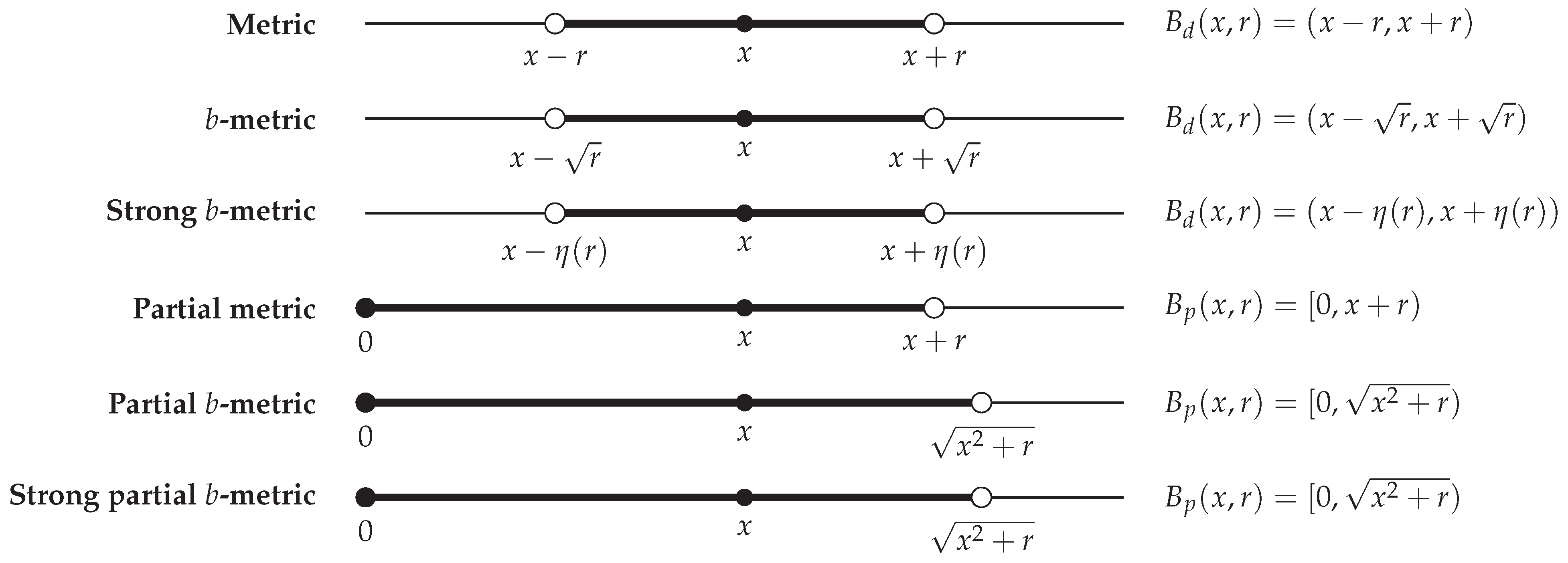
The above examples illustrate the gradual transition from classical metric geometry to generalized metric geometries.

In metric, b-metric, and strong b-metric spaces, every ball is symmetric about its centre Figure 1. In contrast, for partial metric-type spaces, the positive self-distance $p(x,x)$ shifts the defining inequality, so that the centre is no longer the geometric midpoint of the ball Figure 1.

This phenomenon is one of the principal geometric differences between ordinary metric spaces and partial metric-type spaces and explains why their induced topologies possess substantially different properties.

2.4. Point-to-Set Distance and Excess

The contraction condition in the main theorem is formulated for multivalued mappings. For this reason, besides the distance between two points, we also need the distance from a point to a set and the corresponding excess between two sets. These notions play the role of the point-to-set distance and the one-sided Hausdorff excess adapted to strong partial b-metric spaces.

Definition 3.

Let $(X,p,K)$ be a strong partial b-metric space, let $x\in X$, and let $⌀\ne A\subseteq X$. The distance from x to A is defined by $p(x,A)={inf}_{a\in A}p(x,a)$.

Since $A\ne ⌀$ and $p(x,a)\ge 0$ for every $a\in A$, the quantity $p(x,A)$ is well defined and belongs to ${\mathbb{R}}_{+}$.

Example 3.

[Point-to-set distance in the classical metric-type spaces] Consider the set $A=[2,\infty )$ and the point $x=1$. The distance from x to A depends on the underlying generalized metric.

1.

Metric space: Let $d(x,y)=|x-y|$. Then $d(1,A)={inf}_{a\ge 2}|1-a|=1$. Indeed, the infimum is attained at $a=2$.

2.

b-metric space: Let $d(x,y)={|x-y|}^2$. Then $d(1,A)={inf}_{a\ge 2}{(a-1)}^2=1$. Again the minimum is attained at $a=2$.

3.

Strong b-metric space: For $d(x,y)=h\left(\right|x-y\left|\right)$, where $h\left(t\right)=t+{\displaystyle \frac{t^2}{1+t}}$, the minimum distance is attained at $a=2$, and therefore $d(1,A)=h\left(1\right)=1+{\displaystyle \frac{1}{2}}={\displaystyle \frac{3}{2}}$.

4.

Partial metric space: Let $p(x,y)=\max \{x,y\}$. Then $p(1,A)={inf}_{a\ge 2}\max \{1,a\}=2$. Hence $p(1,A)>p(1,1)=1$.

5.

Partial b-metric space: Let $p(x,y)=\max {\{x,y\}}^2$. Then $p(1,A)={inf}_{a\ge 2}\max {\{1,a\}}^2=4$. Since $p(1,1)=1$, the distance from the point to the set exceeds the self-distance.

6.

Strong partial b-metric space: For the standard example

$$(p(x,y)=\left\{\begin{array}{cc}{x}^2,\hfill & x=y,\hfill \\ \max \{x^2,y^2\},\hfill & x\ne y,\hfill \end{array}\right.$$

we obtain $p(1,A)=4$, exactly as in the previous example.

The following definition is motivated by the classical one-sided Pompeiu–Hausdorff excess used in set-valued analysis; see, for example, Aubin and Frankowska [10]. Here, the ordinary metric is replaced by the strong partial b-metric p. A closely related one-sided excess in the setting of strong b-metric spaces is employed in [3].

Definition 4.

Let $(X,p,K)$ be a strong partial b-metric space and let $⌀\ne A,B\subseteq X$. The excess of A over B is defined by ${\delta }_p(A,B)={sup}_{a\in A}p(a,B)$, where $p(a,B)={inf}_{b\in B}p(a,b)$.

Equivalently, ${\delta }_p(A,B)={sup}_{a\in A}{inf}_{b\in B}p(a,b)$.

The value $+\infty$ is allowed whenever the supremum is unbounded.

The excess ${\delta }_p(A,B)$ measures how far the set A extends beyond the set B. In particular, since $p(a,B)\ge 0$ for every $a\in A$, one has ${\delta }_p(A,B)=0$ if and only if $p(a,B)=0$ for every $a\in A$.

Moreover, ${\delta }_p(A,B)$ is not symmetric, so, in general, ${\delta }_p(A,B)\ne {\delta }_p(B,A)$. This asymmetry is natural for multivalued contractions, where one compares the image of one point with the image of another.

Throughout the paper, all excesses appearing in the contractive conditions are finite. This follows automatically from the hypotheses of the main theorem.

Example 4.

[Excess in the classical metric-type spaces] Consider the sets $A=[1,2]$ and $B=[2,3]$. The excess ${\delta }_p(A,B)={sup}_{a\in A}p(a,B)$ depends on the underlying generalized metric.

1.

Metric space: Let $d(x,y)=|x-y|$. For every $a\in [1,2]$, there holds $d(a,B)=2-a$. Hence $\delta (A,B)={sup}_{a\in [1,2]}(2-a)=1$.

2.

b-metric space: Let $d(x,y)={|x-y|}^2$. Then $d(a,B)={(2-a)}^2$, and therefore

$$\delta (A,B)=\underset{a\in [1,2]}{sup}{(2-a)}^2=1.$$

3.

Strong b-metric space: For $d(x,y)=h\left(\right|x-y\left|\right)$, where $h\left(t\right)=t+{\displaystyle \frac{t^2}{1+t}}$, there holds the equality $d(a,B)=h(2-a)$ for every $a\in [1,2]$. Since h is increasing,

$${\delta }_d(A,B)=\underset{a\in [1,2]}{sup}h(2-a)=h\left(1\right)={\displaystyle \frac{3}{2}}.$$

4.

Partial metric space: Let $p(x,y)=\max \{x,y\}$. For every $a\in A$ there holds

$$p(a,B)=\underset{b\in [2,3]}{inf}\max \{a,b\}=2.$$

Consequently, ${\delta }_p(A,B)=2$.

5.

Partial b-metric space: Let $p(x,y)=\max {\{x,y\}}^2$. Then $p(a,B)=4$, for every $a\in A$, and hence ${\delta }_p(A,B)=4$.

6.

Strong partial b-metric space: For

$$p(x,y)=\left\{\begin{array}{cc}{x}^2,\hfill & x=y,\hfill \\ \max \{x^2,y^2\},\hfill & x\ne y,\hfill \end{array}\right.$$

we again obtain $p(a,B)=4$, and therefore ${\delta }_p(A,B)=4$.

2.5. 0-Completeness

The convergence concept naturally associated with strong partial b-metric spaces differs from the classical notion of Cauchy completeness. Since the contractive iteration constructed in the proof of the main theorem produces sequences whose mutual distances converge to zero, the appropriate completeness assumption is 0-completeness. We briefly recall the corresponding definition.

Definition 5.

([1]) A nonempty subset A of $(X,p,K)$ is called 0-closed with respect to p if $p(x,A)=0$ then $x\in A$ for every $x\in X$. We denote by ${\mathcal{C}}_0^p\left(X\right)$ the family of all nonempty subsets of X that are 0-closed with respect to p.

The term 0-closed is used in the zero-distance, or equivalently sequential, sense. It does not refer to closedness with respect to a topology generated by p-balls.

Definition 6.

([1]) A sequence $\left\{x_n\right\}$ in $(X,p,K)$ is called 0-Cauchy if ${lim}_{m,n\to \infty }p(x_m,x_n)=0$.

Definition 7.

([1]) The space $(X,p,K)$ is called 0-complete if every 0-Cauchy sequence $\left\{x_n\right\}$ admits a point $x\in X$ such that $p(x,x)={lim}_{n\to \infty }p(x_n,x)={lim}_{m,n\to \infty }p(x_m,x_n)=0$.

In this case, we say that $\left\{x_n\right\}$ 0-converges to x and write $x_n\stackrel{0}{\to }x$.

Remark 6.

The use of 0-completeness is intrinsic to the fixed point argument developed below. Indeed, the contractive iteration constructed in the proofs satisfies ${lim}_{m,n\to \infty }p(x_m,x_n)=0$, and is therefore 0-Cauchy. The proof only requires the convergence of such sequences to a point $x^{*}\in X$ satisfying $p(x^{*},x^{*})=0$ and $p(x_n,x^{*})⟶0$.

Thus, ordinary Cauchy completeness would be stronger than necessary for the present result.

Moreover, every Cauchy complete strong partial b-metric space is 0-complete, whereas the converse need not hold. Consequently, a fixed point theorem established under 0-completeness applies to a potentially larger class of spaces.

2.6. Bianchini–Grandolfi Gauge Functions

The following notion goes back to the work of Bianchini and Grandolfi [11] and has become standard in nonlinear fixed point theory (see also [?]).

Definition 8.

[11,?] Let $J\subseteq {\mathbb{R}}_{+}$ be an interval containing 0. A strictly increasing mapping $\phi :J⟶J$ will be called a Bianchini–Grandolfi gauge function if it is continuous at 0 and

$$S_{\phi }\left(t\right):={\displaystyle \sum _{k=0}^{\infty }}{\phi }^k\left(t\right)<\infty ,t\in J,$$

where ${\phi }^0\left(t\right)=t$ and ${\phi }^{k+1}\left(t\right)=\phi \left({\phi }^k\left(t\right)\right)$.

The summability condition in Definition 8 implies $\phi \left(0\right)=0$ and $\phi \left(t\right)<t$ for every $t\in J\setminus \left\{0\right\}$.

Indeed, otherwise the terms of the corresponding convergent series would not tend to zero.

3. Auxiliary Estimates

Lemma 1.

Let $(X,p,K)$ be a strong partial b-metric space and let $⌀\ne A\subseteq X$. The following conditions are equivalent:

(i) 

A is 0-closed with respect to p;

(ii) 

whenever $\left\{a_n\right\}\subseteq A$ and $x\in X$ satisfy $p(a_n,x)⟶0$, then $x\in A$.

Moreover, for every $x\in X$, there holds $p(x,A)=0$ if and only if there exists a sequence $\left\{a_n\right\}\subseteq A$ such that $p(x,a_n)⟶0$.

Whenever these equivalent conditions hold for a given x, one necessarily has $p(x,x)=0$.

Proof. 

Assume first that A is 0-closed and let $\left\{a_n\right\}\subseteq A$ satisfy $p(a_n,x)\to 0$ for some $x\in X$. By symmetry and the definition of the distance from a point to a set,

$$0\le p(x,A)\le p(x,a_n)=p(a_n,x).$$

Passing to the limit gives $p(x,A)=0$. The 0-closedness of A therefore implies $x\in A$.

Conversely, suppose that b holds and let $x\in X$ satisfy $p(x,A)=0$. By the definition of the infimum, for every $n\in \mathbb{N}$ there exists $a_n\in A$ such that $p(x,a_n)<{\displaystyle \frac{1}{n}}$.

By symmetry, $p(a_n,x)=p(x,a_n)\to 0$. Condition (ii) yields $x\in A$, and hence A is 0-closed.

The same argument proves the asserted sequential characterization of $p(x,A)=0$. Finally, by (Definition 1 b), $0\le p(x,x)\le p(x,a_n)$. From ${lim}_{n\to \infty }p(x,a_n)=0$ we conclude that $p(x,x)=0$. □

Lemma 2.

Let $x_0,x_1,\dots ,x_n\in X$, where $n\ge 2$. Then

$$p(x_0,x_n)\le p(x_0,x_1)+K{\displaystyle \sum _{j=1}^{n-1}}p(x_j,x_{j+1})-{\displaystyle \sum _{j=1}^{n-1}}p(x_j,x_j)\le p(x_0,x_1)+K{\displaystyle \sum _{j=1}^{n-1}}p(x_j,x_{j+1}).$$

Proof. 

We will prove the inequality by induction by repeatedly applying Definition 1.d to the first term of the preceding estimate.

Step 1: Applying Definition 1.d with $x=x_0$, $y=x_n$, and $z=x_{n-1}$, we obtain

$$\begin{array}{cc}\hfill p(x_0,x_n)& \le p(x_0,x_{n-1})+Kp(x_{n-1},x_n)-p(x_{n-1},x_{n-1}).\hfill \end{array}$$

Step 2: Now apply Definition 1.d only to the term $p(x_0,x_{n-1})$, using $z=x_{n-2}$:

$$\begin{array}{cc}\hfill p(x_0,x_{n-1})& \le p(x_0,x_{n-2})+Kp(x_{n-2},x_{n-1})-p(x_{n-2},x_{n-2}).\hfill \end{array}$$

Substituting this estimate into the previous inequality gives

$$p(x_0,x_n)\le p(x_0,x_{n-2})+Kp(x_{n-2},x_{n-1})+Kp(x_{n-1},x_n)-p(x_{n-2},x_{n-2})-p(x_{n-1},x_{n-1}).$$

Step k: Assume that after $k-1$ substitutions we have reached

$$p(x_0,x_n)\le p(x_0,x_{n-k+1})+K{\displaystyle \sum _{j=n-k+1}^{n-1}}p(x_j,x_{j+1})-{\displaystyle \sum _{j=n-k+1}^{n-1}}p(x_j,x_j).$$

Applying Definition 1.d only to the remaining term $p(x_0,x_{n-k+1})$, with intermediate point $x_{n-k}$, yields

$$p(x_0,x_{n-k+1})\le p(x_0,x_{n-k})+Kp(x_{n-k},x_{n-k+1})-p(x_{n-k},x_{n-k}).$$

Substituting this estimate gives the next step of the iteration.

After $n-1$ iterations we arrive at

$$p(x_0,x_n)\le p(x_0,x_1)+K{\displaystyle \sum _{j=1}^{n-1}}p(x_j,x_{j+1})-{\displaystyle \sum _{j=1}^{n-1}}p(x_j,x_j),$$

which proves the first inequality.

Finally, since $p(x_j,x_j)\ge 0$ for every j, $-{\sum }_{j=1}^{n-1}p(x_j,x_j)\le 0$, and therefore

$$p(x_0,x_n)\le p(x_0,x_1)+K{\displaystyle \sum _{j=1}^{n-1}}p(x_j,x_{j+1}).$$

□

Remark 7.

Definitions 6 and 5, as well as Lemmas 1 and 2, are purely metric. They do not require the family of open p-balls to form a base for a topology. In particular, $overline{B}_p(x_0,r)$ is used only as a localization set, and no topological closure argument is used below.

3.1. Linguistic Illustrative Examples

The linguistic interpretation adopted below follows the distinction between discourse expansion and linguistic enrichment proposed in [4]. A refinement step may introduce a new expression, but it may also remove an inappropriate construction, replace a non-idiomatic phrase, correct a grammatical deficiency, or adapt the formulation to a particular academic purpose. Consequently, the transition between two linguistic states should not be understood as a simple increase in vocabulary size. It represents a qualitative improvement in grammatical accuracy, terminological precision, rhetorical organization, or communicative appropriateness.

This interpretation is particularly relevant to academic discourse, where linguistic competence involves sensitivity to disciplinary conventions and to the rhetorical functions performed by alternative formulations [12,13]. Thus, two expressions may communicate the same mathematical content while differing in formality, explicitness, argumentative strength, or pedagogical orientation. Such differences explain why the model may admit several distinct but equally stable terminal formulations.

Example 5

(A strong b-metric model of linguistic enrichment). Let $X=\{u_0,u_1,u_2,u_3\}$ be a collection of English texts ordered according to increasing linguistic refinement:

$$\begin{array}{cc}\hfill u_0=& “\mathrm{Boy}\mathrm{go}\mathrm{school}\mathrm{yesterday}.”,\hfill \\ \hfill u_1=& “\mathrm{The}\mathrm{boy}\mathrm{went}\mathrm{to}\mathrm{school}\mathrm{yesterday}.”,\hfill \\ \hfill u_2=& “\mathrm{The}\mathrm{young}\mathrm{boy}\mathrm{walked}\mathrm{to}\mathrm{school}\mathrm{yesterday}\mathrm{because}\mathrm{the}\mathrm{weather}\mathrm{was}\mathrm{pleasant}.”,\hfill \\ \hfill u_3=& “\mathrm{Although}\mathrm{the}\mathrm{weather}\mathrm{was}\mathrm{cool},\mathrm{the}\mathrm{young}\mathrm{boy}\mathrm{chose}\mathrm{to}\mathrm{walk}\hfill \\ & \mathrm{to}\mathrm{school},\sin \mathrm{ce}\mathrm{the}\mathrm{quiet}\mathrm{journey}\mathrm{helped}\mathrm{him}\mathrm{prepare}\mathrm{for}\mathrm{the}\mathrm{day}.”.\hfill \end{array}$$

The index of each text represents its linguistic level. Define $q(u_i,u_j)={|i-j|}^2$.

The quantity $q(u_i,u_j)$ measures the structural separation between two linguistic levels. Since X is finite, one verifies directly that $q(u_i,u_j)\le q(u_i,u_k)+5q(u_k,u_j)$ for every $u_i,u_j,u_k\in X$. Hence $(X,q,5)$ is a strong b-metric space.

The interpretation is straightforward. Every text is regarded as complete, and only the linguistic distance between different texts is measured. Passing through an intermediate text may increase the total distance by the factor $K=5$, reflecting the accumulation of translation, editing or interpretation errors during successive revisions.

Example 6

(A strong partial b-metric model of linguistic enrichment). The previous example assumes that every text is already complete. Suppose now that each text still possesses an intrinsic linguistic deficit. Define $h\left(u_0\right)={\displaystyle \frac{3}{2}}$, $h\left(u_1\right)=1$, $h\left(u_2\right)={\displaystyle \frac{1}{2}}$, and $h\left(u_3\right)=0$, where $h\left(u_i\right)$ denotes the amount of grammatical, lexical and discursive refinement that is still required.

Define $d(u_i,u_j)=q(u_i,u_j)+h\left(u_i\right)+h\left(u_j\right)$.

Then $d(u_i,u_i)=2h\left(u_i\right)$, so the self-distance measures the remaining linguistic incompleteness of the corresponding text.

In particular, $d(u_0,u_0)=3$, $d(u_1,u_1)=2$, $d(u_2,u_2)=1$, and $d(u_3,u_3)=0$.

Thus the self-distance is interpreted as the remaining linguistic deficit of the text. In particular, the most elementary text has the largest self-distance, whereas the most developed text has zero self-distance.

The complete distance table is

We show that $(X,d,5)$ is a strong partial b-metric space.

First, d is symmetric because both q and $h\left(u_i\right)+h\left(u_j\right)$ are symmetric in i and j.

Moreover, $d(u_i,u_j)-d(u_i,u_i)=q(u_i,u_j)+h\left(u_j\right)-h\left(u_i\right)\ge 0$, because $h\left(u_i\right)-h\left(u_j\right)\le q(u_i,u_j)$.

Consequently, there holds the inequality $d(u_i,u_i)\le d(u_i,u_j)$.

Suppose that $d(u_i,u_i)=d(u_i,u_j)=d(u_j,u_j)$. Then from the equalities

$$2h\left(u_i\right)=q(u_i,u_j)+h\left(u_i\right)+h\left(u_j\right)=2h\left(u_j\right),$$

it follows that $h\left(u_i\right)=h\left(u_j\right)$ and $q(u_i,u_j)=0$.

Therefore $i=j$, and hence $u_i=u_j$.

Finally, using the strong b-metric inequality for q, we obtain

$$d(u_i,u_j)=q(u_i,u_j)+h\left(u_i\right)+h\left(u_j\right)\le q(u_i,u_k)+5q(u_k,u_j)+h\left(u_i\right)+h\left(u_j\right).$$

On the other hand,

$$\begin{array}{cc}& d(u_i,u_k)+5d(u_k,u_j)-d(u_k,u_k)\hfill \\ & =q(u_i,u_k)+h\left(u_i\right)+h\left(u_k\right)+5\left(q(u_k,u_j)+h\left(u_k\right)+h\left(u_j\right)\right)-2h\left(u_k\right)\hfill \\ & =q(u_i,u_k)+5q(u_k,u_j)+h\left(u_i\right)+5h\left(u_j\right)+4h\left(u_k\right).\hfill \end{array}$$

Since $h\ge 0$, we have $h\left(u_i\right)+h\left(u_j\right)\le h\left(u_i\right)+5h\left(u_j\right)+4h\left(u_k\right)$ and therefore, $d(u_i,u_j)\le d(u_i,u_k)+5d(u_k,u_j)-d(u_k,u_k)$.

Thus $(X,d,5)$ is a strong partial b-metric space.

The transition from the first example to the second illustrates the difference between strong b-metrics and strong partial b-metrics. In a strong b-metric space, every object is assumed to be complete and only the distance between different objects is measured. In a strong partial b-metric space, each object may also possess its own intrinsic incompleteness, represented by its positive self-distance.

Example 7

(A linguistic interpretation of the excess functional). Let X denote a collection of English texts equipped with a strong partial b-metric p. Assume that the value $p(x,y)$ measures the overall linguistic dissimilarity between two texts, taking into account their grammatical correctness, lexical richness, structural complexity, and the remaining linguistic incompleteness represented by the self-distance $p(x,x)$.

Let $A=\{a_1,a_2,a_3\}$ be a collection of texts produced by a learner,

$$\begin{array}{cc}\hfill a_1& =“\mathrm{The}\mathrm{student}\mathrm{solve}\mathrm{the}\mathrm{problem}.”,\hfill \\ \hfill a_2& =“\mathrm{The}\mathrm{student}\mathrm{solved}\mathrm{problem}\mathrm{by}\mathrm{induction}.”,\hfill \\ \hfill a_3& =“\mathrm{Student}\mathrm{use}\mathrm{theorem}\mathrm{because}\mathrm{function}\mathrm{continuous}.”,\hfill \end{array}$$

and let $B=\{b_1,b_2,b_3\}$ be a family of linguistically acceptable target texts,

$$\begin{array}{cc}\hfill b_1& =“\mathrm{The}\mathrm{student}\mathrm{solves}\mathrm{the}\mathrm{problem}.”,\hfill \\ \hfill b_2& =“\mathrm{The}\mathrm{student}\mathrm{solved}\mathrm{the}\mathrm{problem}\mathrm{by}\mathrm{induction}.”,\hfill \\ \hfill b_3& =“\mathrm{The}\mathrm{student}\mathrm{uses}\mathrm{the}\mathrm{theorem}\mathrm{because}\mathrm{the}\mathrm{function}\mathrm{is}\mathrm{continuous}.”.\hfill \end{array}$$

Suppose that the linguistic distances between the learner texts and the target texts are given by

4. Main Result

4.1. A Local Set-Valued Fixed Point Theorem

Theorem 1.

Let $(X,p,K)$ be a 0-complete strong partial b-metric space. Let $x_0\in X$, $r>0$, and let $F:{\overline{B}}_p(x_0,r)⟶{\mathcal{C}}_0^{p}zero\left(X\right)$ be a set-valued mapping. Let $J\subseteq {\mathbb{R}}_{+}$ be an interval containing 0, and let $\phi :J⟶J$ be a Bianchini–Grandolfi gauge function.

Assume that there exists $\alpha \in J\setminus \left\{0\right\}$ such that

$$p(x_0,F\left(x_0\right))<\alpha$$

(6)

and

$$K{S}_{\phi }\left(\alpha \right)-(K-1)\alpha \le p(x_0,x_0)+r.$$

(7)

Suppose further that

$${\delta }_p\left(F\left(x\right)\cap {\overline{B}}_p(x_0,r),F\left(y\right)\right)\le \phi \left(p(x,y)\right)$$

(8)

for all distinct $x,y\in {\overline{B}}_p(x_0,r)$ such that $p(x,y)\in J$ and $F\left(x\right)\cap {\overline{B}}_p(x_0,r)\ne ⌀$.

Then F has a fixed point $x^{*}\in {\overline{B}}_p(x_0,r)$, i.e., $x^{*}\in F\left(x^{*}\right)$.

If F is single-valued and

$$Kp(x_0,x_0)+(K+1)r\in J,$$

(9)

then $x^{*}$ is the unique fixed point of F in ${\overline{B}}_p(x_0,r)$.

Proof. 

Since $S_{\phi }\left(\alpha \right)=\alpha +{\sum }_{j=1}^{\infty }{\phi }^j\left(\alpha \right)$, condition (7) is equivalent to

$$\alpha +K{\displaystyle \sum _{j=1}^{\infty }}{\phi }^j\left(\alpha \right)\le p(x_0,x_0)+r.$$

(10)

By (6) and the definition of the infimum, there exists $x_1\in F\left(x_0\right)$ such that

$$p(x_0,x_1)<\alpha .$$

(11)

Condition (10) gives $p(x_0,x_1)<p(x_0,x_0)+r$, so $x_1\in {\overline{B}}_p(x_0,r)$. If $x_1=x_0$, then $x_0\in F\left(x_0\right)$, and the existence assertion follows. Assume therefore that $x_1\ne x_0$.

Since $x_1\in F\left(x_0\right)\cap {\overline{B}}_p(x_0,r)$, condition (8) yields

$$p(x_1,F\left(x_1\right))\le {\delta }_p\left(F\left(x_0\right)\cap {\overline{B}}_p(x_0,r),F\left(x_1\right)\right)\le \phi \left(p(x_0,x_1)\right)<\phi \left(\alpha \right).$$

Hence, there exists $x_2\in F\left(x_1\right)$ such that $p(x_1,x_2)<\phi \left(\alpha \right)$.

We construct the sequence and verify its localization simultaneously. Suppose that $x_0,\dots ,x_n$ have been chosen so that

$$x_{j+1}\in F\left(x_j\right),p(x_j,x_{j+1})<{\phi }^j\left(\alpha \right),0\le j\le n-1,$$

and

$$x_j\in {\overline{B}}_p(x_0,r),0\le j\le n.$$

Case I) If $x_n=x_{n-1}$, then $x_n\in F\left(x_{n-1}\right)=F\left(x_n\right)$, and a fixed point has been obtained.

Case II) Assume that $x_n\ne x_{n-1}$. Since $0\le p(x_{n-1},x_n)<{\phi }^{n-1}\left(\alpha \right)\le \alpha$ and J is an interval containing 0 and $\alpha$, we have $p(x_{n-1},x_n)\in J$.

Moreover, $x_n\in F\left(x_{n-1}\right)\cap {\overline{B}}_p(x_0,r)$ and thus,

$$p(x_n,F\left(x_n\right))\le {\delta }_p\left(F\left(x_{n-1}\right)\cap {\overline{B}}_p(x_0,r),F\left(x_n\right)\right)\le \phi \left(p(x_{n-1},x_n)\right)<{\phi }^n\left(\alpha \right).$$

We may therefore choose $x_{n+1}\in F\left(x_n\right)$ such that

$$p(x_n,x_{n+1})<{\phi }^n\left(\alpha \right).$$

(12)

By Lemma 2,

$$\begin{array}{cc}\hfill p(x_0,x_{n+1})& \le p(x_0,x_1)+K{\displaystyle \sum _{j=1}^n}p(x_j,x_{j+1})-{\displaystyle \sum _{j=1}^n}p(x_j,x_j)\hfill \\ & \le p(x_0,x_1)+K{\displaystyle \sum _{j=1}^n}p(x_j,x_{j+1})<\alpha +K{\displaystyle \sum _{j=1}^n}{\phi }^j\left(\alpha \right)\hfill \\ & \le p(x_0,x_0)+r.\hfill \end{array}$$

Consequently, $x_{n+1}\in {\overline{B}}_p(x_0,r)$.

Thus, either a fixed point is obtained after finitely many steps, or there exists a sequence $\left\{x_n\right\}$ such that

$$x_{n+1}\in F\left(x_n\right),p(x_n,x_{n+1})<{\phi }^n\left(\alpha \right),n\ge 0,$$

(13)

and $x_n\in {\overline{B}}_p(x_0,r)$ for every $n\ge 0$.

Let $n>m$. By Lemma 2,

$$\begin{array}{cc}\hfill p(x_m,x_n)& \le p(x_m,x_{m+1})+K{\displaystyle \sum _{j=m+1}^{n-1}}p(x_j,x_{j+1})-{\displaystyle \sum _{j=m+1}^{n-1}}p(x_j,x_j)\hfill \\ & \le p(x_m,x_{m+1})+K{\displaystyle \sum _{j=m+1}^{n-1}}p(x_j,x_{j+1})<{\phi }^m\left(\alpha \right)+K{\displaystyle \sum _{j=m+1}^{n-1}}{\phi }^j\left(\alpha \right)\hfill \\ & \le K{\displaystyle \sum _{j=m}^{\infty }}{\phi }^j\left(\alpha \right).\hfill \end{array}$$

Because of $S_{\phi }\left(\alpha \right)<\infty$, there holds ${lim}_{m\to \infty }{\sum }_{j=m}^{\infty }{\phi }^j\left(\alpha \right)=0$ and thus

$$\underset{m,n\to \infty }{lim}p(x_m,x_n)=0.$$

Hence, $\left\{x_n\right\}$ is 0-Cauchy.

By the 0-completeness of $(X,p,K)$, there exists $x^{*}\in X$ such that

$$p(x^{*},x^{*})=0\mathrm{and}p(x_n,x^{*})⟶0.$$

(14)

By (IV), we can write $p(x_0,x^{*})\le p(x_0,x_n)+Kp(x_n,x^{*})-p(x_n,x_n)$. Since $p(x_n,x_n)\ge 0$, passing to the limit gives $p(x_0,x^{*})\le p(x_0,x_0)+r$ and therefore, $x^{*}\in {\overline{B}}_p(x_0,r)$.

It remains to prove that $x^{*}\in F\left(x^{*}\right)$.

Case I) If $x_{n-1}=x^{*}$ for all sufficiently large n, then also $x_n=x^{*}$ for all sufficiently large n. Since $x_n\in F\left(x_{n-1}\right)$, we obtain $x^{*}\in F\left(x^{*}\right)$.

Case II) Otherwise, there exists a subsequence, still denoted by $\left\{x_{n-1}\right\}$, such that $x_{n-1}\ne x^{*}$.

Since $p(x_{n-1},x^{*})⟶0$ and J is an interval containing 0 and $\alpha >0$, we have $p(x_{n-1},x^{*})\in J$ for all sufficiently large n.

Moreover, $x_n\in F\left(x_{n-1}\right)\cap {\overline{B}}_p(x_0,r)$.

Condition (8) therefore gives

$$p(x_n,F\left(x^{*}\right))\le {\delta }_p\left(F\left(x_{n-1}\right)\cap {\overline{B}}_p(x_0,r),F\left(x^{*}\right)\right)\le \phi \left(p(x_{n-1},x^{*})\right).$$

For every $u\in F\left(x^{*}\right)$, condition (iv) implies

$$p(x^{*},u)\le p(x^{*},x_n)+Kp(x_n,u)-p(x_n,x_n).$$

Taking the infimum over $u\in F\left(x^{*}\right)$, and then omitting the nonpositive term ″$-p{(x_n,x_n)}^{″}$, we obtain

$$p(x^{*},F\left(x^{*}\right))\le p(x^{*},x_n)+Kp(x_n,F\left(x^{*}\right)).$$

Consequently,

$$p(x^{*},F\left(x^{*}\right))\le p(x^{*},x_n)+K\phi \left(p(x_{n-1},x^{*})\right).$$

Letting $n\to \infty$ in the above inequality, using (14), the continuity of $\phi$ at 0, and $\phi \left(0\right)=0$, we obtain $p(x^{*},F\left(x^{*}\right))=0$.

Since $F\left(x^{*}\right)$ is 0-closed with respect to p, Definition 5 yields $x^{*}\in F\left(x^{*}\right)$. This proves the existence assertion.

Finally, suppose that F is single-valued and let $u,v\in {\overline{B}}_p(x_0,r)$ be fixed points of F. By (d),

$$\begin{array}{cc}\hfill p(u,v)& \le p(u,x_0)+Kp(x_0,v)-p(x_0,x_0)\hfill \\ & \le p(x_0,x_0)+r+K\left(p(x_0,x_0)+r\right)-p(x_0,x_0)=Kp(x_0,x_0)+(K+1)r.\hfill \end{array}$$

Since J is an interval containing 0, condition (9) implies $p(u,v)\in J$.

If $u\ne v$, condition (8) yields $p(u,v)={\delta }_p(\left\{u\right\},\left\{v\right\})\le \phi \left(p(u,v)\right)<p(u,v)$, which is impossible.

Therefore $u=v$, and the fixed point is unique. □

Example 8

(A local model of linguistic enrichment). Let X denote the collection of all linguistic productions that may occur during a learning process. Each element of X is regarded as a complete text rather than an isolated sentence. Assume that $(X,p,K)$ is a 0-complete strong partial b-metric space, where the distance $p(x,y)$ measures the overall linguistic discrepancy between two texts, while the self-distance $p(x,x)$ represents the remaining linguistic incompleteness of the text x.

Suppose that a learner starts from an initial linguistic state $x_0\in X$. For a prescribed radius $r>0$, the closed ball ${\overline{B}}_p(x_0,r)$ contains all texts that can realistically be reached during the current stage of instruction. Thus, the learning process is assumed to remain within a local neighbourhood of the initial linguistic competence.

For every text $x\in {\overline{B}}_p(x_0,r)$, let $F\left(x\right)\subseteq X$ denote the family of all linguistically acceptable immediate revisions of x. Since a text may admit several equally appropriate improvements, the mapping F is naturally set-valued.

The initial condition (6) expresses the existence of at least one feasible linguistic improvement of the initial production.

The condition (7) guarantees that the cumulative effect of successive linguistic refinements never leaves the prescribed local learning region.

The contractive condition (8) has a natural educational interpretation. It requires that whenever two texts are linguistically similar, their corresponding families of acceptable revisions are also close. In other words, similar linguistic productions should generate similar pedagogical recommendations. This condition ensures the coherence and stability of the learning strategy.

The conclusion of Theorem 1 asserts the existence of a text $x^{*}\in {\overline{B}}_p(x_0,r)$ such that $x^{*}\in F\left(x^{*}\right)$. From the linguistic point of view, this means that the learning process reaches a locally stable linguistic state. At this stage, the current text already belongs to the family of its own admissible revisions, so no further essential linguistic modification is required within the given learning environment.

If the mapping F is single-valued, then the theorem guarantees that this stable linguistic state is unique inside the prescribed local region. For the prescribed initial state satisfying the hypotheses of the theorem, the single-valued iterative trajectory constructed in the proof is uniquely determined and 0-converges to this local fixed point. The theorem does not assert convergence from every arbitrary initial state of the localization region.

4.2. Construction of a Strong Partial b-Metric for Linguistic Enrichment

We now develop a finite linguistic model illustrating the abstract framework of the preceding theorem. The construction is carried out in three steps.

First, the linguistic states are organized as the vertices of a weighted graph, and the corresponding shortest-path distance provides an ordinary metric. Second, this metric is transformed into a strong b-metric by means of a nonlinear increasing function. Third, a prescribed family of stable linguistic states is used to introduce positive self-distances, thereby producing a strong partial b-metric.

The resulting construction has a direct linguistic interpretation. The graph metric measures the minimum number of normalized revision steps between two formulations. The strong b-metric assigns additional weight to larger linguistic transitions, while the self-distance of a state measures its remaining distance from the stable target family.

The construction may be summarized as

$$\mathrm{weighted}\mathrm{revision}\mathrm{graph}⟶\mathrm{metric}⟶\mathrm{strong}b-\mathrm{metric}⟶\mathrm{strong}\mathrm{partial}b-\mathrm{metric}.$$

We begin with two general construction results and then apply them to a finite family of progressively enriched linguistic states.

4.2.1. From a Metric to a Strong b-Metric

Every metric is trivially a strong b-metric with any coefficient $K\ge 1$. However, this observation does not produce a genuinely new distance. The following result gives a nonlinear construction that may fail to satisfy the ordinary triangle inequality while retaining the strong b-metric inequality.

Theorem 2.

Let $(X,d)$ be a bounded metric space and let $D=sup\left\{d\right(x,y):x,y\in X\}<\infty$. Let $q>1$ and $\lambda >0$. Define $d_{q,\lambda }(x,y)=d(x,y)+\lambda d{(x,y)}^q$ for $x,y\in X$.

Then $d_{q,\lambda }$ is a strong b-metric on X with coefficient $K=1+\lambda q{\left(2D\right)}^{q-1}$, i.e.,

$$d_{q,\lambda }(x,z)\le d_{q,\lambda }(x,y)+K{d}_{q,\lambda }(y,z)$$

for all $x,y,z\in X$.

In general, $d_{q,\lambda }$ need not be a metric.

Proof. 

Put $h\left(t\right)=t+\lambda t^q$ for $t\ge 0$. Then $\rho (x,y)=h\left(d\right(x,y\left)\right)$.

The function h is strictly increasing, $h\left(0\right)=0$, and therefore $\rho$ is symmetric and $\rho (x,y)=0$ if and only if $x=y$.

Let $a=d(x,y)$ and $b=d(y,z)$. By the metric triangle inequality, there holds $d(x,z)\le a+b$. Since $a,b\le D$, we have $a+b\le 2D$. By the mean value theorem, the equality

$$h(a+b)-h\left(a\right)=h^{\prime }\left(\xi \right)b$$

holds for some $\xi \in [a,a+b]\subseteq [0,2D]$. Since $h^{\prime }\left(t\right)=1+\lambda q{t}^{q-1}$ it follows that

$$h^{\prime }\left(\xi \right)\le 1+\lambda q{\left(2D\right)}^{q-1}=K.$$

Therefore, $h(a+b)\le h\left(a\right)+Kb$. Form $b\le h\left(b\right)$ we get $h(a+b)\le h\left(a\right)+Kh\left(b\right)$.

Consequently,

$$\rho (x,z)=h\left(d\right(x,z\left)\right)\le h(a+b)\le h\left(a\right)+Kh\left(b\right)=\rho (x,y)+K\rho (y,z).$$

Thus, $\rho$ is a strong b-metric with coefficient K. □

The boundedness assumption is automatic in the finite linguistic model considered below. The transformation $t⟼t+\lambda t^q$ preserves the order of the original distances but gives additional weight to larger separations. Thus, a transition across several linguistic levels is penalized more strongly than a transition between neighbouring levels.

Corollary 1.

Let $(X,d)$ be a metric space of finite diameter D, and let $\lambda >0$. Then

$$\rho (x,y)=d(x,y)+\lambda d{(x,y)}^2$$

is a strong b-metric with coefficient $K=1+4\lambda D$.

4.2.2. From a Strong b-Metric to a Strong Partial b-Metric

The preceding construction measures the distance between distinct states but assigns zero self-distance to every state. To model the remaining incompleteness of an intermediate linguistic formulation, we now prescribe a nonempty target family A of stable states.

The distance $\rho (x,A)={inf}_{a\in A}\rho (x,a)$ from x to A, measures the smallest remaining linguistic transition required to reach an admissible stable formulation. We use this value as the self-distance of x.

Theorem 3.

Let $(X,\rho ,K)$ be a strong b-metric space and $A\subseteq X$ be nonempty. Put $\rho (x,A)={inf}_{a\in A}\rho (x,a)$ and define

$$p_A(x,y)=\rho (x,y)+\max \{\rho (x,A),\rho (y,A)\}.$$

Then $p_A$ is a strong partial b-metric on X with coefficient K.

Moreover, $p_A(x,x)=\rho (x,A)$ for every $x\in X$.

Proof. 

For brevity, put $w\left(x\right)=\rho (x,A)$. Since $\rho (x,x)=0$, we have

$$p_A(x,x)=\rho (x,x)+\max \{w\left(x\right),w\left(x\right)\}=w\left(x\right)=\rho (x,A).$$

We verify the axioms of a strong partial b-metric.

First,

$$p_A(x,y)=\rho (x,y)+\max \{w\left(x\right),w\left(y\right)\}\ge w\left(x\right)=p_A(x,x).$$

Thus, the small self-distance condition is satisfied.

The symmetry of $p_A$ follows immediately from the symmetry of $\rho$:

$$p_A(x,y)=p_A(y,x).$$

Suppose that $p_A(x,x)=p_A(x,y)=p_A(y,y)$. Then $w\left(x\right)=w\left(y\right)$. Furthermore,

$$w\left(x\right)=\rho (x,y)+\max \left\{w\right(x),w(y\left)\right\}=\rho (x,y)+w\left(x\right).$$

Hence, $\rho (x,y)=0$. Since $\rho$ separates points, it follows that $x=y$. The converse implication is immediate.

It remains to verify the strong partial b-metric inequality. Since $\rho$ is a strong b-metric,

$$\rho (x,z)\le \rho (x,y)+K\rho (y,z).$$

For arbitrary nonnegative numbers $a,b,c$, we have

$$\max \{a,c\}\le \max \{a,b\}+\max \{b,c\}-b.$$

Applying this inequality to $a=w\left(x\right)$,$b=w\left(y\right)$, and $c=w\left(z\right)$, we obtain

$$\max \left\{w\right(x),w(z\left)\right\}\le \max \left\{w\right(x),w(y\left)\right\}+\max \left\{w\right(y),w(z\left)\right\}-w\left(y\right).$$

Since $K\ge 1$, there holds

$$\max \left\{w\right(y),w(z\left)\right\}\le K\max \left\{w\right(y),w(z\left)\right\}.$$

Consequently,

$$\begin{array}{cc}\hfill p_A(x,z)& =\rho (x,z)+\max \left\{w\right(x),w(z\left)\right\}\hfill \\ & \le \rho (x,y)+K\rho (y,z)+\max \left\{w\right(x),w(y\left)\right\}+K\max \left\{w\right(y),w(z\left)\right\}-w\left(y\right)\hfill \\ & =p_A(x,y)+K{p}_A(y,z)-p_A(y,y).\hfill \end{array}$$

Therefore, $p_A$ is a strong partial b-metric with coefficient K. □

The construction separates two kinds of information. The term $\rho (x,y)$ measures the difference between the particular formulations x and y, whereas $\max \left\{\rho \right(x,A),\rho (y,A\left)\right\}$ records their remaining distance from the stable target family.

In particular, $p_A(x,x)=\rho (x,A)$. Thus, positive self-distance is no longer introduced by an arbitrary assignment of numerical weights. It is generated by the geometry of the underlying revision process.

Corollary 2.

Under the assumptions of Theorem 3, suppose additionally that $x\in A$, provided that $\rho (x,A)=0$. Then $p_A(x,x)=0$ if and only if $x\in A$.

Proof. 

By the definition of $p_A$, there holds $p_A(x,x)=\rho (x,A)$. If $x\in A$, then

$$0\le \rho (x,A)\le \rho (x,x)=0.$$

Conversely, if $p_A(x,x)=0$, then $\rho (x,A)=0$, and the assumed zero-closedness gives $x\in A$. □

Corollary 3.

Let $(X,d)$ be a metric space with finite diameter $D=diam\left(X\right)$. Let $q>1$, $\lambda >0$, and let $A\subseteq X$ be nonempty. Define $\rho (x,y)=d(x,y)+\lambda d{(x,y)}^q$ and

$$p_A(x,y)=\rho (x,y)+\max \{\rho (x,A),\rho (y,A)\}.$$

Then $p_A$ is a strong partial b-metric with coefficient $K=1+\lambda q{\left(2D\right)}^{q-1}$ and there holds

$$p_A(x,x)=\rho (x,A)=\underset{a\in A}{inf}\left(d(x,a)+\lambda d{(x,a)}^q\right).$$

The preceding results apply to any bounded metric space and any nonempty target family. We now specialize them to the twenty linguistic states used in the enrichment model. Their organization into successive levels determines a weighted revision graph and hence an ordinary shortest-path metric.

4.2.3. A Graph Metric on the Linguistic States

Let $\mathcal{A}=\{a_1,\dots ,a_{20}\}$ and consider the partition $\mathcal{A}=L_0\cup L_1\cup L_2\cup L_3\cup L_4\cup L_5$, where

$$\begin{array}{cc}\hfill L_0& =\{a_1,a_2,a_3,a_4\},\hfill \\ \hfill L_1& =\{a_5,a_6,a_7,a_8\},\hfill \\ \hfill L_2& =\{a_9,a_{10},a_{11},a_{12}\},\hfill \\ \hfill L_3& =\{a_{13},a_{14},a_{15},a_{16}\},\hfill \\ \hfill L_4& =\{a_{17},a_{18}\},\hfill \\ \hfill L_5& =\{a_{19},a_{20}\}.\hfill \end{array}$$

Construct an undirected weighted graph whose vertex set is $\mathcal{A}$. Every vertex in $L_i$ is joined to every vertex in $L_{i+1}$, for $i=0,\dots ,4$, and every edge has length ${\displaystyle \frac{1}{5}}$.

Let $d(a,b)$ be the length of a shortest path joining a and b. Then d is a metric on $\mathcal{A}$.

More explicitly, if $a\in L_i$ and $b\in L_j$, then

$$d(a,b)=\left\{\begin{array}{cc}0,\hfill & a=b,\hfill \\ {\displaystyle \frac{|i-j|}{5}},\hfill & i\ne j,\hfill \\ {\displaystyle \frac{2}{5}},\hfill & i=j,a\ne b.\hfill \end{array}\right.$$

Since the largest separation occurs between $L_0$ and $L_5$, we have $diam(\mathcal{A},d)=1$. The metric d therefore records the normalized number of refinement levels separating two linguistic states.

4.2.4. The Stable Target Family and the Induced Self-Distances

We now apply the constructions in two preceding theorems and Section 4.2.3. Choose $q=2$, $\lambda =1$, and define $\rho (a,b)=d(a,b)+d{(a,b)}^2$.

Since $diam(\mathcal{A},d)=1$, Corollary 1 shows that $\rho$ is a strong b-metric with coefficient $K=1+4diam(\mathcal{A},d)=5$.

Let $A=L_5=\{a_{19},a_{20}\}$ be the prescribed stable target family. Define $p(a,b)=\rho (a,b)+\max \left\{\rho \right(a,A),\rho (b,A\left)\right\}$. By Theorem 3, p is a strong partial b-metric with coefficient $K=5$.

Indeed, states belonging to different levels are connected by a shortest path passing through the intermediate levels. Two distinct states at the same level are connected by a path through an adjacent level and therefore have distance $2/5$.

Consequently,

$$p(a,a)=\left\{\begin{array}{cc}2,\hfill & a\in L_0,\hfill \\ {\displaystyle \frac{36}{25}},\hfill & a\in L_1,\hfill \\ {\displaystyle \frac{24}{25}},\hfill & a\in L_2,\hfill \\ {\displaystyle \frac{14}{25}},\hfill & a\in L_3,\hfill \\ {\displaystyle \frac{6}{25}},\hfill & a\in L_4,\hfill \\ 0,\hfill & a\in L_5.\hfill \end{array}\right.$$

The successive values 2, ${\displaystyle \frac{36}{25}}$, ${\displaystyle \frac{24}{25}}$, ${\displaystyle \frac{14}{25}}$, ${\displaystyle \frac{6}{25}}$, and 0 measure the decreasing distance from the corresponding refinement levels to the stable target family. They are not assigned independently to the states; they are obtained from the graph metric and the chosen nonlinear transformation.

Thus, the linguistic interpretation of the self-distance is determined by the structure of the revision graph:

$$p(a,a)=\mathrm{the}\mathrm{transformed}\mathrm{shortest}\mathrm{distance}\mathrm{from}a\mathrm{to}\mathrm{a}\mathrm{stable}\mathrm{text}.$$

The graph metric measures the minimum number of normalized revision steps required to move between two linguistic states. The nonlinear transformation assigns a larger weight to transitions between more distant refinement levels, while the resulting self-distance measures the remaining linguistic effort required to reach at least one stable formulation.

Thus, the displayed self-distances decrease strictly along the refinement levels.

The two states $a_{19}$ and $a_{20}$ have zero self-distance because they are stable. Nevertheless,

$$p(a_{19},a_{20})=\rho (a_{19},a_{20})={\displaystyle \frac{2}{5}}+{\left({\displaystyle \frac{2}{5}}\right)}^2={\displaystyle \frac{14}{25}}>0.$$

Therefore, the two stable formulations remain distinct despite having zero self-distance.

4.2.5. Linguistic Realization of the Abstract States

We now complete the abstract construction by assigning a concrete linguistic formulation to each state $a_i$. All twenty formulations express the same mathematical statement, but differ in grammatical accuracy, terminological precision, logical explicitness, and stylistic appropriateness. Thus, membership in the same level indicates a comparable degree of refinement, not linguistic identity.

Example 9.

[A multistage linguistic enrichment process] Retain the state space $X=\mathcal{A}$, its levels $L_0,\dots ,L_5$, the stable family $A=L_5$, and the strong partial b-metric p constructed in Subsection 4.2.3 and Subsection 4.2.4.

We next verify that $(X,p,5)$ is 0-complete. Let $\left\{x_n\right\}\subseteq X$ be a 0-Cauchy sequence. Since X is finite and $p(x,y)>0$ whenever $x\ne y$, the sequence must eventually be constant. If its eventual value is x, then the 0-Cauchy property gives $p(x,x)=0$. Therefore $x\in L_5$. Hence, every 0-Cauchy sequence 0-converges to a point of $L_5$, and $(X,p,5)$ is 0-complete.

Define the set-valued revision mapping $F:X⟶{\mathcal{C}}_0^p\left(X\right)$ by $F\left(a\right)=L_{i+1}$, provided that $a\in L_i$ for $\le i\le 4$, and $F\left(a\right)=L_5$ for $a\in L_5$.

Thus, every nonterminal state is mapped to the entire next refinement level, while every stable state is mapped to the stable target family. The mapping is genuinely set-valued.

Every nonempty subset of X is 0-closed with respect to p. Indeed, suppose that $B\subseteq X$ is nonempty and $p(x,B)=0$.

Since B is finite, there exists $b\in B$ such that $p(x,b)=0$.

The definition of p implies $\rho (x,b)=0$. Since $\rho$ separates points, $x=b$, and hence $x\in B$. Therefore, $F\left(a\right)\in {\mathcal{C}}_0^p\left(X\right)$ for every $a\in X$.

Let $J=[0,\infty )$ and define $\phi \left(t\right)={\displaystyle \frac{6}{7}}t$.

Then $\phi :J\to J$ is strictly increasing, satisfies $\phi \left(t\right)<t$ for every $t>0$, and ${\phi }^n\left(t\right)={\left({\displaystyle \frac{6}{7}}\right)}^{n}t$.

Moreover, $S_{\phi }\left(t\right)={\sum }_{n=0}^{\infty }{\phi }^n\left(t\right)={\displaystyle \frac{t}{1-\frac{6}{7}}}=7t$ and thus $\phi$ is a Bianchini–Grandolfi gauge function.

We now verify the contractive condition. Put $s\left(i\right)=min\{i+1,5\}$ for $i=0,\dots ,5$. Then $F\left(x\right)=L_{s\left(i\right)}$ whenever $x\in L_i$.

Just for convenience, let us put $r_i=\rho (x,A)$ for $x\in L_i$. Therefore, $r_i$ is precisely the self-distance already listed for the level $L_i$.

If $x\in L_i$, $y\in L_j$, and $i\ne j$, then $p(x,y)=h\left({\displaystyle \frac{|i-j|}{5}}\right)+\max \{r_i,r_j\}$, where $h\left(t\right)=t+t^2$.

If $x,y\in L_i$ are distinct, then

$$p(x,y)=h\left({\displaystyle \frac{2}{5}}\right)+r_i={\displaystyle \frac{14}{25}}+r_i.$$

Similarly,

$${\delta }_p(F\left(x\right),F\left(y\right))=\left\{\begin{array}{cc}{r}_{s\left(i\right)},\hfill & s\left(i\right)=s\left(j\right),\hfill \\ h\left({\displaystyle \frac{\left|s\right(i)-s(j\left)\right|}{5}}\right)+\max \{r_{s\left(i\right)},r_{s\left(j\right)}\},\hfill & s\left(i\right)\ne s\left(j\right).\hfill \end{array}\right.$$

For distinct $x\in L_i$ and $y\in L_j$, define

$$R_{ij}={\displaystyle \frac{{\delta }_p(F\left(x\right),F\left(y\right))}{p(x,y)}}.$$

The quotient depends only on the corresponding refinement levels. Its values are

where the diagonal entries correspond to distinct states belonging to the same level.

The largest value is ${\max }_{0\le i,j\le 5}{R}_{ij}={\displaystyle \frac{36}{43}}<{\displaystyle \frac{6}{7}}$ and consequently,

$${\delta }_p(F\left(x\right),F\left(y\right))\le {\displaystyle \frac{6}{7}}p(x,y)=\phi \left(p(x,y)\right)$$

for all distinct $x,y\in X$.

To demonstrate the genuinely local character of Theorem 1, we now apply it on a proper subset of X. Choose $x_0=a_{17}$, $\alpha ={\displaystyle \frac{1}{2}}$, and $r={\displaystyle \frac{11}{20}}$. Since $a_{17}\in L_4$ and $F\left(a_{17}\right)=L_5$, we have

$$p(a_{17},F\left(a_{17}\right))=p(a_{17},L_5)={\displaystyle \frac{12}{25}}<{\displaystyle \frac{1}{2}}=\alpha .$$

There holds $p(a_{17},a_{17})+r={\displaystyle \frac{6}{25}}+{\displaystyle \frac{11}{20}}={\displaystyle \frac{79}{100}}$.

For $a_{19},a_{20}\in L_5$, the inequality $p(a_{17},a_{19})=p(a_{17},a_{20})={\displaystyle \frac{12}{25}}<{\displaystyle \frac{79}{100}}$ holds.

For every $x\in L_0\cup L_1\cup L_2\cup L_3$ there hold

$$p(a_{17},a_{18})={\displaystyle \frac{4}{5}},p(a_{17},x)\ge {\displaystyle \frac{4}{5}}$$

Consequently, ${\overline{B}}_p\left(a_{17},{\displaystyle \frac{11}{20}}\right)=\{a_{17},a_{19},a_{20}\}⊊X$

For this local application, define the Bianchini–Grandolfi gauge $\psi \left(t\right)={\displaystyle \frac{1}{10}}t$ for $t\in [0,\infty )$.

Then $S_{\psi }\left(t\right)={\displaystyle \frac{t}{1-\frac{1}{10}}}={\displaystyle \frac{10}{9}}t$.

For every $x\in {\overline{B}}_p(a_{17},11/20)$, one has $F\left(x\right)=L_5$. Hence, for all distinct $x,y\in {\overline{B}}_p(a_{17},11/20)$, there holds

$${\delta }_p\left(F\left(x\right)\cap {\overline{B}}_p(a_{17},11/20),F\left(y\right)\right)={\delta }_p(L_5,L_5)=0\le \psi \left(p(x,y)\right).$$

Finally, since $K=5$, we get $K{S}_{\psi }\left(\alpha \right)-(K-1)\alpha =5·{\displaystyle \frac{10}{9}}·{\displaystyle \frac{1}{2}}-4·{\displaystyle \frac{1}{2}}={\displaystyle \frac{7}{9}}$ and furthermore, ${\displaystyle \frac{7}{9}}<{\displaystyle \frac{79}{100}}=p(a_{17},a_{17})+{\displaystyle \frac{11}{20}}$.

Thus, all assumptions of Theorem 1 are satisfied on the proper localization set

$${\overline{B}}_p\left(a_{17},{\displaystyle \frac{11}{20}}\right)=\{a_{17},a_{19},a_{20}\}.$$

Consequently, F has a fixed point in this proper local ball.

In fact, $F\left(a_{19}\right)=F\left(a_{20}\right)=L_5=\{a_{19},a_{20}\}$ and hence

$$a_{19}\in F\left(a_{19}\right),a_{20}\in F\left(a_{20}\right).$$

No state in $L_0\cup \dots \cup L_4$ belongs to its own image. Therefore, $Fix\left(F\right)=\{a_{19},a_{20}\}$.

The mapping describes the multistage enrichment process

$$L_0⟶L_1⟶L_2⟶L_3⟶L_4⟶L_5.$$

At every nonterminal stage, the image $F\left(a\right)$ contains all admissible formulations at the next refinement level. Different choices may therefore generate different enrichment trajectories, but every trajectory eventually reaches the stable family $L_5$.

The self-distance $p(a,a)=\rho (a,L_5)$ measures the transformed shortest distance from the current linguistic state to the stable target family. It decreases strictly from one refinement level to the next and vanishes exactly on the stable states $a_{19}$ and $a_{20}$.

Remark 8.

[Linguistic interpretation] The construction above models linguistic enrichment as a multistage process in which a formulation may admit several equally acceptable revisions at each stage. Consequently, the mapping F is multivalued: it does not prescribe a unique successor, but allows different revision trajectories leading toward the stable target family.

The self-distance has a global rather than a local interpretation. It measures the remaining linguistic effort required to reach a stable formulation, not merely the effort associated with the next revision step. Its strict decrease along the refinement levels therefore represents the progressive reduction of the grammatical, terminological, logical, and stylistic deficiencies of the text.

The presence of two terminal states also distinguishes stabilization from uniqueness. The states $a_{19}$ and $a_{20}$ may represent, for example, a concise formal formulation and a more explanatory, pedagogically oriented formulation of the same mathematical statement. Both are stable because no further essential revision is required within the adopted model, but they remain distinct because they serve different communicative purposes. Thus, convergence to the stable target family does not require all admissible enrichment trajectories to produce the same final text.

Example 10.

[Linguistic realization of the abstract states] We now assign a concrete linguistic formulation to each abstract state $a_i$ introduced in Example 9. All formulations express the same underlying mathematical statement: a continuous real-valued function on a closed and bounded interval attains both its minimum and its maximum.

The formulations are arranged according to the previously defined levels $L_0,L_1,\dots ,L_5$. States belonging to the same level have a comparable degree of linguistic refinement, although they may differ in vocabulary, notation, sentence structure, or communicative style.

The first level, $L_0=\{a_1,a_2,a_3,a_4\}$, contains initial formulations with substantial grammatical, terminological, and structural deficiencies.

State $a_1$: If function is continuous in closed interval, it have minimum and maximum in this interval.

State $a_2$: When a function continuous on a closed interval, then there exist a smallest and a biggest value of the function.

State $a_3$: For every continuous function in closed and bounded interval, the minimum and maximum are existing.

State $a_4$: A continuous function over a closed interval always has one minimum value and one maximum value somewhere inside the interval.

The formulations in $L_0$ convey the intended general idea, but they contain errors involving articles, subject–verb agreement, prepositions, word formation, or mathematical precision. Moreover, they do not clearly distinguish between the extreme values of the function and the points at which these values are attained. The first application of F therefore represents a principally corrective stage.

The second level, $L_1=\{a_5,a_6,a_7,a_8\}$, contains grammatically improved formulations in which the principal mathematical objects are identified more clearly.

State $a_5$: If a function is continuous on a closed interval, it has a minimum and a maximum value on that interval.

State $a_6$: Every function that is continuous on a closed and bounded interval has both a smallest value and a largest value.

State $a_7$: A continuous real function defined on a closed interval reaches its minimum and maximum values on the interval.

State $a_8$: When a real-valued function is continuous on a closed bounded interval, its minimum and maximum values exist on this interval.

The texts in $L_1$ are largely grammatical, but some expressions remain less appropriate for mathematical discourse. For instance, the verbs “has,” “reaches,” and “exists” communicate the intended meaning, but they are less precise than the standard mathematical verb “attains.” The transition from $L_1$ to $L_2$ therefore primarily concerns terminological refinement.

The third level, $L_2=\{a_9,a_{10},a_{11},a_{12}\}$, introduces more accurate mathematical terminology and a clearer description of the domain.

State $a_9$: Every continuous real-valued function on a closed and bounded interval attains a minimum value and a maximum value.

State $a_{10}$: If a real-valued function is continuous on a compact interval, then it attains both its smallest and its largest values on that interval.

State $a_{11}$: A function that is continuous on a closed interval $[a,b]$ attains its minimum and maximum somewhere in $[a,b]$.

State $a_{12}$: Let f be a continuous real-valued function on a closed and bounded interval. Then the range of f contains a least element and a greatest element.

At this level, the formulations are mathematically meaningful and mostly precise. Nevertheless, some versions do not explicitly identify points of the domain at which the extreme values are attained, whereas others use correct but unnecessarily indirect set-theoretic terminology. The next refinement therefore makes the logical and quantificational structure more explicit.

The fourth level, $L_3=\{a_{13},a_{14},a_{15},a_{16}\}$, contains academically structured formulations that explicitly relate the extreme values to points of the interval.

State $a_{13}$: If $f:[a,b]\to \mathbb{R}$ is continuous, then there exist points $x_{min},x_{\max }\in [a,b]$ such that

$$f\left(x_{min}\right)\le f\left(x\right)\le f\left(x_{\max }\right)$$

for every $x\in [a,b]$.

State $a_{14}$: Let f be continuous on the closed interval $[a,b]$. Then f attains both an absolute minimum and an absolute maximum on $[a,b]$.

State $a_{15}$.For every continuous function $f:[a,b]\to \mathbb{R}$, there exist $u,v\in [a,b]$ satisfying

$$f\left(u\right)=\underset{x\in [a,b]}{min}f\left(x\right)\mathrm{and}f\left(v\right)=\underset{x\in [a,b]}{\max }f\left(x\right).$$

State $a_{16}$: A continuous real-valued function defined on a compact interval attains its extreme values; that is, it has both an absolute minimum and an absolute maximum on its domain.

The texts in $L_3$ are grammatically correct and mathematically precise. They differ mainly in notation, degree of formality, and choice of terminology. Accordingly, the transition to $L_4$ is largely stylistic rather than corrective.

The fifth level, $L_4=\{a_{17},a_{18}\}$, contains nearly final versions corresponding to two different communicative orientations.

State $a_{17}$: Let $f:[a,b]\to \mathbb{R}$ be continuous. Then there exist $x_{min},x_{\max }\in [a,b]$ such that

$$f\left(x_{min}\right)=\underset{x\in [a,b]}{min}f\left(x\right)\mathit{and}f\left(x_{\max }\right)=\underset{x\in [a,b]}{\max }f\left(x\right).$$

State $a_{18}$: Suppose that a real-valued function is continuous on a closed and bounded interval. Then the function takes both a smallest value and a largest value at some points of that interval.

The formulation $a_{17}$ is oriented toward concise formal mathematical writing, whereas $a_{18}$ is intended as an explanatory version for readers who may be less familiar with symbolic notation. The last application of F performs a final stylistic refinement without changing the mathematical content.

Finally, $L_5=\{a_{19},a_{20}\}$, contains two stable formulations.

State $a_{19}$ stable formal formulation: Let $f:[a,b]\to \mathbb{R}$ be continuous. Then f attains its minimum and maximum on $[a,b]$; equivalently, there exist $x_{min},x_{\max }\in [a,b]$ such that

$$f\left(x_{min}\right)\le f\left(x\right)\le f\left(x_{\max }\right)$$

for every $x\in [a,b]$.

State $a_{20}$ stable explanatory formulation: Every continuous real-valued function on a closed and bounded interval takes both a smallest and a largest value. In other words, there are points in the interval at which the function attains its absolute minimum and its absolute maximum.

Both $a_{19}$ and $a_{20}$ are grammatically correct, mathematically accurate, and stylistically appropriate. Neither is linguistically superior in an absolute sense. The first is more suitable for a formal theorem or proof, whereas the second is more appropriate for teaching or explanatory exposition.

In accordance with the abstract construction, $p(a_{19},a_{19})=p(a_{20},a_{20})=0$. Thus, neither stable formulation has a positive remaining distance to a further level of refinement. At the same time, $p(a_{19},a_{20})>0$, so the two formulations remain distinct. This illustrates that zero self-distance expresses stabilization within the model, not the identity of all stable outcomes.

The multivalued mapping F models the fact that the editing process does not determine a unique successor at any intermediate stage. Starting from $x\in L_i$, any element of $L_{i+1}$ is regarded as an admissible next formulation. Hence different sequences of linguistic choices may lead to different stable texts:

$$L_0⟶L_1⟶L_2⟶L_3⟶L_4⟶L_5.$$

Along every such trajectory, the self-distances decrease, and for each $x\in L_i$, $0\le i\le 4$, the value $p(x,x)=\rho (x,L_5)$ quantifies the transformed remaining distance to the stable target family, whereas the immediate next-level distance is $p(x,L_{i+1})=p(x,x)+6/25$.

5. Special Cases of the Main Theorem

The following corollaries show that several well-known classes of contractive mappings arise as direct special cases of Theorem 1.

Corollary 4

(Local linear set-valued contraction). Let $(X,p,K)$ be a 0-complete strong partial b-metric space, let $x_0\in X$ and $r>0$, and let $F:{\overline{B}}_p(x_0,r)⟶{\mathcal{C}}_0^p\left(X\right)$. Suppose that there exist $q\in (0,1)$ and $\alpha >0$ such that

$$p(x_0,F\left(x_0\right))<\alpha$$

(15)

and

$$\alpha +{\displaystyle \frac{Kq\alpha }{1-q}}\le p(x_0,x_0)+r.$$

(16)

Assume further that

$${\delta }_p\left(F\left(x\right)\cap {\overline{B}}_p(x_0,r),F\left(y\right)\right)\le qp(x,y)$$

(17)

for all distinct $x,y\in {\overline{B}}_p(x_0,r)$ such that $F\left(x\right)\cap {\overline{B}}_p(x_0,r)\ne ⌀$.

Then F has a fixed point $x^{*}\in {\overline{B}}_p(x_0,r)$.

If F is single-valued, then $x^{*}$ is the unique fixed point of F in ${\overline{B}}_p(x_0,r)$.

Proof. 

Define $\phi \left(t\right)=qt$ for $t\in {\mathbb{R}}_{+}$. Since $q\in (0,1)$, the mapping $\phi$ is strictly increasing, continuous at 0, and ${\phi }^n\left(t\right)=q^{n}t$.

Consequently, $S_{\phi }\left(t\right)={\sum }_{n=0}^{\infty }{q}^{n}t={\displaystyle \frac{t}{1-q}}$. Therefore,

$$K{S}_{\phi }\left(\alpha \right)-(K-1)\alpha ={\displaystyle \frac{K\alpha }{1-q}}-(K-1)\alpha =\alpha +{\displaystyle \frac{Kq\alpha }{1-q}}.$$

Thus, condition (16) is precisely the localization condition in Theorem 1. Moreover, (17) becomes

$${\delta }_p\left(F\left(x\right)\cap {\overline{B}}_p(x_0,r),F\left(y\right)\right)\le \phi \left(p(x,y)\right).$$

Hence, all the assumptions of Theorem 1 are satisfied.

Since here $J={\mathbb{R}}_{+}$, the additional condition for uniqueness is automatic. Therefore, if F is single-valued, its fixed point is unique in ${\overline{B}}_p(x_0,r)$. □

Example 11

(Linear linguistic improvement). Corollary 4 describes a learning process in which each instructional step produces a uniform proportional improvement of the learner’s linguistic competence. Let X denote the collection of all possible linguistic productions, equipped with a strong partial b-metric p. For every text x, the set $F\left(x\right)$ consists of all linguistically acceptable revisions that may be obtained after one stage of instruction.

The contractive condition (17) expresses a one-sided contractive relation between the corresponding families of admissible revisions. More precisely, every element of $F\left(x\right)\cap {\overline{B}}_p(x_0,r)$ has point-to-set distance to $F\left(y\right)$ bounded above by $qp(x,y)$.

Consequently, the condition does not assert that every possible pair of revisions is at distance at most $qp(x,y)$. Rather, each admissible revision associated with the first state can be approximated by a revision associated with the second state in accordance with the prescribed one-sided point-to-set estimate.

Along the iterative selection constructed in the proof, the successive step sizes are controlled geometrically, while the chain estimate ensures that the selected trajectory remains inside the prescribed local learning region.

Corollary 4 guarantees the existence of a stable linguistic state $x^{*}$, while its proof constructs an admissible iterative selection that 0-converges to such a fixed point. In this state, $x^{*}\in F\left(x^{*}\right)$, meaning that the current linguistic production already satisfies the requirements of the instructional model and no further essential local revision is required.

If the revision operator is single-valued, then this stable linguistic state is unique. For the prescribed initial state satisfying the hypotheses of the corollary, the resulting single-valued iterative trajectory converges to this unique local fixed point. No assertion is made here about convergence from every arbitrary initial state of the local region.

Corollary 5

(Partial metric case). Let $(X,p)$ be a 0-complete partial metric space, let $x_0\in X$ and $r>0$, and let $F:{\overline{B}}_p(x_0,r)⟶{\mathcal{C}}_0^p\left(X\right)$. Let $J\subseteq {\mathbb{R}}_{+}$ be an interval containing 0, and let $\phi :J⟶J$ be a Bianchini–Grandolfi gauge function.

Assume that there exists $\alpha \in J\setminus \left\{0\right\}$ such that

$$p(x_0,F\left(x_0\right))<\alpha$$

(18)

and

$$S_{\phi }\left(\alpha \right)\le p(x_0,x_0)+r.$$

(19)

Suppose further that

$${\delta }_p\left(F\left(x\right)\cap {\overline{B}}_p(x_0,r),F\left(y\right)\right)\le \phi \left(p(x,y)\right)$$

(20)

for all distinct $x,y\in {\overline{B}}_p(x_0,r)$ such that $p(x,y)\in J$ and $F\left(x\right)\cap {\overline{B}}_p(x_0,r)\ne ⌀$.

Then F has a fixed point $x^{*}\in {\overline{B}}_p(x_0,r)$.

If F is single-valued and

$$p(x_0,x_0)+2r\in J,$$

(21)

then $x^{*}$ is the unique fixed point of F in ${\overline{B}}_p(x_0,r)$.

Proof. 

A partial metric is a strong partial b-metric with coefficient $K=1$. Therefore,

$$K{S}_{\phi }\left(\alpha \right)-(K-1)\alpha =S_{\phi }\left(\alpha \right),$$

while the uniqueness condition in Theorem 1 becomes

$$Kp(x_0,x_0)+(K+1)r=p(x_0,x_0)+2r.$$

The conclusion now follows directly from Theorem 1. □

Corollary 6

(Local Banach-type principle). Let $(X,p,K)$ be a 0-complete strong partial b-metric space, let $x_0\in X$ and $r>0$, and let $T:{\overline{B}}_p(x_0,r)⟶{\overline{B}}_p(x_0,r)$ be a single-valued mapping. Suppose that there exist $q\in (0,1)$ and $\alpha >0$ such that

$$p(x_0,T{x}_0)<\alpha$$

(22)

and

$$\alpha +{\displaystyle \frac{Kq\alpha }{1-q}}\le p(x_0,x_0)+r.$$

(23)

If

$$p(Tx,Ty)\le qp(x,y)$$

(24)

for all distinct $x,y\in {\overline{B}}_p(x_0,r)$, then T has a unique fixed point in ${\overline{B}}_p(x_0,r)$.

Proof. 

Define the set-valued mapping $F\left(x\right):=\left\{Tx\right\}$ for $x\in {\overline{B}}_p(x_0,r)$.

Every singleton is 0-closed with respect to p. Indeed, if $p(z,\{Tx\left\}\right)=p(z,Tx)=0$, then, by (b), there holds $p(z,z)=p(Tx,Tx)=0$. By (a) we conclude that $z=Tx$.

Since T maps ${\overline{B}}_p(x_0,r)$ into itself, $F\left(x\right)\cap {\overline{B}}_p(x_0,r)=\left\{Tx\right\}$. Consequently,

$${\delta }_p\left(F\left(x\right)\cap {\overline{B}}_p(x_0,r),F\left(y\right)\right)={\delta }_p(\left\{Tx\right\},\left\{Ty\right\})=p(Tx,Ty)\le qp(x,y).$$

The result now follows from Corollary 4. □

Corollary 7

(Global set-valued fixed point principle). Let $(X,p,K)$ be a 0-complete strong partial b-metric space, $F:X⟶{\mathcal{C}}_0^p\left(X\right)$, and $\phi :{\mathbb{R}}_{+}⟶{\mathbb{R}}_{+}$ be a Bianchini–Grandolfi gauge function. Suppose that

$${\delta }_p(F\left(x\right),F\left(y\right))\le \phi \left(p(x,y)\right)$$

(25)

for all distinct $x,y\in X$.

Then F has a fixed point in X. If F is single-valued, then the fixed point is unique.

Proof. 

Fix an arbitrary point $x_0\in X$. Since $F\left(x_0\right)$ is nonempty and p is finite-valued, we have $p(x_0,F\left(x_0\right))<\infty$.

Choose $\alpha >0$ such that $p(x_0,F\left(x_0\right))<\alpha$ Since $S_{\phi }\left(\alpha \right)<\infty$, we may choose $r>0$ sufficiently large so that $K{S}_{\phi }\left(\alpha \right)-(K-1)\alpha \le p(x_0,x_0)+r$.

Consider the restriction of F to ${\overline{B}}_p(x_0,r)$. For all distinct $x,y\in {\overline{B}}_p(x_0,r)$ such that $F\left(x\right)\cap {\overline{B}}_p(x_0,r)\ne ⌀$, we have $F\left(x\right)\cap {\overline{B}}_p(x_0,r)\subseteq F\left(x\right)$. Therefore,

$${\delta }_p\left(F\left(x\right)\cap {\overline{B}}_p(x_0,r),F\left(y\right)\right)\le {\delta }_p(F\left(x\right),F\left(y\right))\le \phi \left(p(x,y)\right).$$

Thus, all the assumptions of Theorem 1 are satisfied with $J={\mathbb{R}}_{+}$ and Consequently, F has a fixed point $x^{*}\in {\overline{B}}_p(x_0,r)\subseteq X$.

Suppose now that F is single-valued and let $u,v\in X$ be fixed points of F. If $u\ne v$, then

$$p(u,v)={\delta }_p(\left\{u\right\},\left\{v\right\})={\delta }_p(F\left(u\right),F\left(v\right))\le \phi \left(p(u,v)\right)<p(u,v),$$

which is impossible. Therefore, $u=v$. □

Corollary 8

(Global linear set-valued contraction). Let $(X,p,K)$ be a 0-complete strong partial b-metric space, and let $F:X⟶{\mathcal{C}}_0^p\left(X\right)$. Suppose that there exists $q\in (0,1)$ such that ${\delta }_p(F\left(x\right),F\left(y\right))\le qp(x,y)$ for all distinct $x,y\in X$.

Then F has a fixed point in X. If F is single-valued, then the fixed point is unique.

Proof. 

Set $\phi \left(t\right)=qt$ for $t\in {\mathbb{R}}_{+}$. Then $S_{\phi }\left(t\right)={\sum }_{n=0}^{\infty }{q}^{n}t={\displaystyle \frac{t}{1-q}}<\infty$.

Thus, $\phi$ is a Bianchini–Grandolfi gauge function, and the conclusion follows from Corollary 7. □

6. Discussion

The main result extends local fixed point theory for multivalued mappings to (0)-complete strong partial (b)-metric spaces. The combination of a nonzero self-distance, a relaxed triangle inequality, and set-valued images requires a proof strategy that differs from the standard arguments used in metric spaces. In particular, the iterative sequence must be constructed in such a way that all its elements remain inside the prescribed localization set. The chain estimate developed in this paper serves two purposes simultaneously: it controls the position of the iterates relative to the initial point and proves that the sequence is (0)-Cauchy.

An important feature of the theorem is that the closed ball is used only as a localization set. No assumption is imposed that the family of (p)-balls forms a basis for a topology, and no topological closure argument is required in the final step of the proof. Instead, the existence of a fixed point follows from (0)-completeness and the (0)-closedness of the values of the mapping. This distinction is relevant because the geometric and topological behavior of balls in partial (b)-metric-type spaces may differ substantially from that of ordinary metric balls. The result therefore separates the localization mechanism from additional topological properties that are not needed for the fixed point argument.

The use of a Bianchini–Grandolfi gauge function provides greater flexibility than a contraction condition determined by a single constant. The summability of the iterates of the gauge function gives the quantitative control required for both localization and convergence. Linear contractions appear as a particularly transparent special case, but the general formulation also covers nonlinear rates of contraction. The corollaries derived from the main theorem clarify its relation to partial metric, Banach-type, and global set-valued fixed point principles.

The construction of a strong partial (b)-metric from a bounded metric space and a prescribed target family constitutes a second contribution of the paper. It provides a systematic way to generate nonzero self-distances with a direct interpretation. The self-distance of a point is determined by its remaining transformed distance to the target family and vanishes precisely on that family. Consequently, the construction is suitable for processes in which stabilization is associated with reaching any member of a collection of admissible terminal states rather than one uniquely prescribed endpoint.

This target-family approach also clarifies the distinction between stability and uniqueness. Several elements may have zero self-distance and may simultaneously be fixed points of a multivalued mapping while remaining mutually distinct. Thus, zero self-distance should not be interpreted as an identification of all stable elements. It indicates only that no further essential transition is required relative to the chosen model. This feature may be useful in applications involving alternative solutions, equivalent representations, or several acceptable outcomes.

The linguistic example illustrates this interpretation in a finite and explicit setting. Alternative formulations of the same mathematical statement are arranged into successive refinement levels, and the revision graph represents admissible transitions between them. The multivalued mapping reflects the fact that linguistic revision is generally nonunique: at a given stage, several grammatically or stylistically acceptable improvements may be available. The two stable states demonstrate that different final texts may express the same mathematical content while serving different communicative purposes. For instance, one formulation may prioritize formal concision, whereas another may emphasize explanation and pedagogical accessibility.

The linguistic construction should be regarded as a mathematical model of the structure of a revision process rather than as an empirical model of language acquisition or text editing. The refinement levels, edge weights, and admissible transitions are prescribed in advance, and the model does not claim that linguistic effort can be measured universally by fixed numerical values. Its purpose is to demonstrate how the abstract notions of self-distance, multivalued transition, and nonunique stabilization can receive a coherent interpretation in language dynamics. An empirical application would require criteria for classifying texts, estimating transition costs, and validating the resulting refinement structure using linguistic data or expert assessment.

Several extensions are possible. On the theoretical side, the local principle may be investigated for other classes of gauge functions, alternative set-distance functionals, coupled or tripled fixed points, common fixed points, and best proximity points. It would also be useful to determine whether some of the localization assumptions can be weakened while preserving the invariance of the iterative sequence. On the applied side, the finite linguistic model could be extended by allowing transitions between nonconsecutive levels, assigning nonuniform revision costs, or permitting the target family to change according to genre, audience, or communicative purpose. Such developments may provide a basis for more detailed mathematical models of linguistic refinement, automated text revision, and other multistage processes with multiple acceptable stable outcomes.

7. Conclusion

A local set-valued fixed point principle has been established in a 0-complete strong partial b-metric space. The proof avoids topological closure arguments and relies instead on 0-closed values of the mapping. The chain estimate in Lemma 2 is essential: it simultaneously guarantees that the iterative sequence remains in the prescribed localization set and that the sequence is 0-Cauchy. Further developments may include coupled, tripled, or n-tupled fixed point results and best proximity point versions of the local principle.

References

- Moshokoa, S.P.; Ncongwane, F.T. On completeness in strong partial b-metric spaces, strong b-metric spaces and the 0-Cauchy completions. Topol. Its Appl. 2020, 275, 107011. [Google Scholar] [CrossRef]
- Ge, X.; Lin, S. Balls in generalizations of metric spaces. J. Inequal. Appl. 2016, 2016, 16. [Google Scholar] [CrossRef]
- Slimani, B.; Graef, J.R.; Ouahab, A. Multivalued contraction fixed-point theorem in b-metric spaces. Mathematics 2024, 12, 567. [Google Scholar] [CrossRef]
- Georgiev, V.; Ilchev, A.; Ivanova, V.; Todorov, A.; Zlatanov, B. Beyond discourse expansion: A linguistic enrichment framework for academic language development. Preprints 2026, 2026080489. [Google Scholar] [CrossRef]
- Beckner, C.; Blythe, R.; Bybee, J.; Christiansen, M.H.; Croft, W.; Ellis, N.C.; Holland, J.; Ke, J.; Larsen-Freeman, D.; Schoenemann, T. Language is a complex adaptive system: Position paper. Lang. Learn. 2009, 59 (Suppl. 1), 1–26. [Google Scholar] [CrossRef]
- Hiver, P.; Al-Hoorie, A.H.; Evans, R. Complex dynamic systems theory in language learning: A scoping review of 25 years of research. Stud. Second Lang. Acquis. 2022, 44(4), 913–941. [Google Scholar] [CrossRef]
- Shukla, S. Partial b-metric spaces and fixed point theorems. Mediterr. J. Math. 2014, 11, 703–711. [Google Scholar] [CrossRef]
- Matthews, S.G. Partial metric topology. Ann. N. Y. Acad. Sci. 1994, 728, 183–197. [Google Scholar] [CrossRef]
- Czerwik, S. Contraction mappings in b-metric spaces. Acta Math. Et. Inform. Univ. Ostrav. 1993, 1, 5–11. [Google Scholar]
- Aubin, J.-P.; Frankowska, H. Set-Valued Analysis. In Systems & Control: Foundations & Applications; Birkhäuser: Boston, MA, USA, 1990; Vol. 2. [Google Scholar]
- Bianchini, R.M.T.; Grandolfi, M. Trasformazioni di tipo contrattivo generalizzato in uno spazio metrico. Atti della Accademia Nazionale dei Lincei. Rendiconti della Classe di Scienze Fisiche, Matematiche e Naturali 1968, 45, 212–216. [Google Scholar]
- Hyland, K. Academic Discourse: English in a Global Context; Continuum: London, UK, 2009. [Google Scholar]
- Schleppegrell, M.J. The Language of Schooling: A Functional Linguistics Perspective; Lawrence Erlbaum Associates: Mahwah, NJ, USA, 2004. [Google Scholar]
Figure 1.
Schematic comparison of open balls generated by the classical metric-type structures considered in Example 2. The drawing is not to scale. Filled endpoints are included, whereas hollow endpoints are excluded. In the metric, b-metric, and strong b-metric cases, the centre x is the midpoint of the interval. For the partial metric-type spaces, the positive self-distance shifts the defining inequality, and x is no longer the geometric midpoint of the ball.
Disclaimer/Publisher’s Note: The statements, opinions and data contained in all publications are solely those of the individual author(s) and contributor(s) and not of MDPI and/or the editor(s). MDPI and/or the editor(s) disclaim responsibility for any injury to people or property resulting from any ideas, methods, instructions or products referred to in the content. |
© 2026 by the authors. Licensee MDPI, Basel, Switzerland. This article is an open access article distributed under the terms and conditions of the Creative Commons Attribution (CC BY) license (http://creativecommons.org/licenses/by/4.0/).
Copyright: This open access article is published under a Creative Commons CC BY 4.0 license, which permit the free download, distribution, and reuse, provided that the author and preprint are cited in any reuse.