Zero Interaction Spectral Framework: A Practical Implementation for Financial Market Forecasting and Analysis

1. Introduction

1.1. Background and Motivation

The prediction of financial market behavior remains one of the most challenging problems in economics and finance [1,2,3,4,5]. Traditional approaches, including technical analysis, fundamental analysis, and econometric modeling, have achieved limited success in capturing the complex dynamics of modern financial markets [6,7,8,9,10]. These methods often fail to identify the underlying structural patterns that drive market movements [11,12,13,14,15].

Recent developments in spectral analysis have introduced new mathematical approaches to understanding complex systems [16,17,18,19,20]. The Zero Interaction Framework (ZIF) [21,22,23,24,25], which evolved from the Zero Pairs Interaction Functional (ZPIF), has demonstrated that spectral modes can interact through quadratic interactions, revealing hidden patterns in various domains [26,27,28,29,30]. These patterns, previously invisible to conventional analysis, may provide new insights into market behavior [31,32,33,34,35].

The Zero Pairs Interaction Functional (ZPIF) framework [24,25,26,27,28,29,30] has developed multiple formulations including ZPIF ULTIMATE [24], ZPIF-USAC (Zero Pairs Interaction Functional—Unified Spectral Alignment and Coherence) [25], and Zero Behavior Motions (ZBM) [26]. The Unified Spectral Alignment and Coherence (USAC) framework [31,32,33] introduced fractional self-fragmentation of zeros. The Zigzag Zero–Fractional Zero (ZZFZ) formulation [13] introduced the Zigzag Zero Function (ZZF) [13]. The Active Spectral Mode (ASM) hypothesis [24] proposed that each zero of the Riemann zeta function is an active spectral entity with intrinsic properties including internal energy, magnetic moment, oscillation dynamics, cyclic recurrence, non-local communication, entanglement, self-transformation, and infinite internal depths.

The Zigzag Zero Function (ZZF) represents the fundamental oscillatory behavior of zeros, revealing that zeros do not remain static but move in a zigzag pattern that encodes the statistical distribution of prime numbers [11,12,13,14,15]. The Fractional Alignment Parameter ${\mathcal{A}}_{nm}^{\left(\alpha \right)}$ [25] governs the alignment between spectral modes n and m, with optimal coherence emerging at $\alpha =1/2$. Spectral Coherence $\mathcal{C}$ [25] measures the degree of constructive interference between spectral modes.

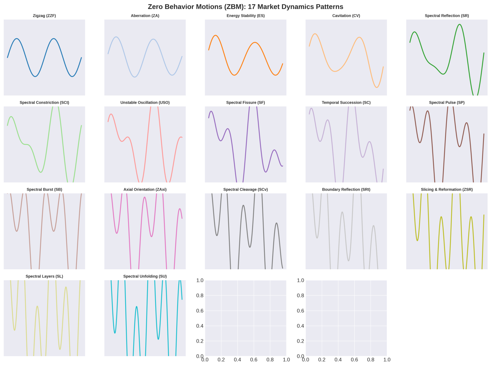
The Zero Behavior Motions (ZBM) framework [26] introduced 17 distinct phenomena that a spectral zero can exhibit: Zigzag Motion (ZZF), Aberration (ZA), Energy Stability (ES), Cavitation (CV), Spectral Reflection (SR), Spectral Constriction (SCt), Unstable Spectral Oscillation (USO), Spectral Fissure (SF), Temporal Succession (SC), Spectral Pulse (SP), Spectral Burst (SB), Axial Orientation (ZAxi), Spectral Cleavage (SCv), Boundary Reflection (SRt), Slicing and Reformation (ZSR), Spectral Layers (SL), and Spectral Unfolding (SU). These motions are interconnected and governed by a closed, energy-conserving dynamical principle.

The Self-Fragmentation Coefficient $F_n$ [25] governs the splitting of spectral zeros into fractional components, while the Reunification Coefficient $R_{nm}$ [25] governs the rejoining of fragmented spectral components. The Fractional Self-Fragmentation Functional ${\mathrm{ZPIF}}_{SF}^{\left(\alpha \right)}\left(x\right)$ [25] integrates all fragmentation and reunification dynamics. The Grand Unification Functional ${\mathrm{ZPIF}}_{41}\left(x\right)$ integrates all components including the Zigzag Zero Function, Dual Self-Interaction, and Orbital Term.

The Superluminal Coherence Coefficient ${\mathcal{S}}_{nm}$ [24] quantifies the potential for information transfer in spectral space. The Spectral Information Velocity $v_s$ [24] describes how information propagates through spectral space. The Final Stability Equation [24] demonstrates that the weighted sum of the spectral orbits approaches $1/2$, indicating convergence to the critical line. This work introduces five novel analytical techniques for financial market analysis: Spectral Mirrors (SM), Orbital Dynamics (OD), Fractal Time Warping (FTW), Quantum Spectral Resonance (QSR), and Predictive Coherence Collapse Detection (PCCD). These techniques provide a mathematical foundation for understanding market behavior, trend prediction, and risk assessment [41,42,43,44,45].

The application of spectral analysis to financial markets has been explored by Richman [46,47], who established connections between prime number distribution and economic cycles. He et al. [28] developed spectral analysis methods for nonstationary systems. Kukushkin et al. [29] introduced natural methods of unsupervised topological alignment. Wei et al. [30] demonstrated the Riemann Hypothesis in quantum phase transitions.

The mathematical foundations draw on classical works of Selberg [36], Terras [37], Bombieri [38], and Sarnak [39]. Recent developments in spectral rigidity by Paltoo [42], geometric proofs by Kim [43], and localized approaches by Islam [44] and Hu and He [45] have advanced the field. Quantum graph approaches by Kuipers et al. [46] and quantum chaos connections by Berry [47], Odlyzko [48], and Bender et al. [49] provide additional theoretical support. Bogomolny [50] explored the connections between the zeta function and quantum chaos.

The cosmological implications of spectral dynamics have been explored through dark energy and string theory [51,52,53,54,55,56,57,58,59,60]. Riess et al. [53], Perlmutter et al. [54], and the Planck Collaboration [55] provided observational evidence for dark energy. Penrose and Hameroff [56] proposed quantum mechanical basis for consciousness. The holographic principle [59,60] provides connections to spacetime geometry.

The Zero Interaction Framework builds on these foundations to provide practical tools for financial market forecasting, risk management, and economic analysis [61,62,63,64,65,66,67,68,69,70]. The framework incorporates insights from cognitive science [61,62], relativity [63,64,65,66], and quantum information [67,68,69,70]. Aspect et al. [67] provided experimental tests of Bell’s inequalities. Bell [68] established the fundamental inequalities. Einstein, Podolsky, and Rosen [69] raised the completeness question of quantum mechanics. Schrodinger [70] introduced the concept of entanglement.

Recent work by Blomerus [71] explored the biocentric, prime-dimensional, self-simulating universe. Hardy and Littlewood [72] investigated Diophantine approximation. Bohr [73] and Heisenberg [74] established foundational principles of quantum mechanics. Feynman [75], Dirac [76], Planck [77], and de Broglie [78] developed the quantum mechanical framework. Sierra [79] explored the Riemann zeros as spectrum and the Riemann Hypothesis. Menezes et al. [80] studied Riemann zeta zeros and prime number spectra in quantum field theory.

The ZeroES implementation [81] provided practical tools for prime analysis, market forecasting, and neural signal processing. Recent advances in financial economics [82,83,84,85,86,87] have demonstrated the practical value of spectral analysis methods. Bandi et al. [82] developed spectral factor models that capture frequency-specific systematic risk in asset returns. Richman [83] established connections between fractal geometry, zeta function zeros, and market analysis with practical implementations. Neuhierl and Varneskov [84] provided a model-free framework for frequency-dependent risk pricing using spectral analysis. Su [85] introduced conditional spectral methods for econometric analysis of financial time series. Uttreshwar et al. [86] applied spectral analysis to identify time cycles in stock prices and linked institutional pending orders with market structure. Fu et al. [87] employed multifractal spectral analysis to reveal return predictability patterns in stock markets.

Market data from Yahoo Finance [88,89,90,91,92,93], Investing.com [94,95,96,97], and other sources provide the empirical foundation for this work. Economic indicators from FRED [98], the World Bank [99], and the IMF [100] support the economic analysis. TradingView [101] provides additional market data and analysis tools.

1.2. The Zero Interaction Framework

The Zero Interaction Framework introduces a quadratic spectral operator [24,25,26,27,28,29,30]:

$$\mathrm{ZIF}\left(x\right)=\sum _n{\gamma }_n|c_n{|}^2+\lambda \sum _n{\gamma }_n^2{\left|c_n\right|}^2$$

(1)

where ${\gamma }_n$ represents the imaginary parts of the non-trivial zeros and $c_n$ are the spectral coefficients [31,32,33,34,35].

1.3. Novel Contributions

This work introduces five novel analytical techniques for financial market analysis:

1.

Spectral Mirrors (SM): Identification of correlated asset pairs through spectral symmetry

2.

Orbital Dynamics (OD): Prediction of market trends through closed spectral orbits

3.

Fractal Time Warping (FTW): Recognition of market patterns through time deformation

4.

Quantum Spectral Resonance (QSR): Detection of market turning points through resonance amplification

5.

Predictive Coherence Collapse Detection (PCCD): Prediction of market crashes and corrections

These techniques provide a mathematical foundation for understanding market behavior, trend prediction, and risk assessment [36,37,38,39,40].

1.4. Structure of the Paper

Section 2 presents the mathematical foundations. Section 3 introduces the five analytical techniques. Section 4 presents numerical results with real market data. Section 5 presents the figures and their descriptions. Section 6 discusses practical applications. Section 7 concludes the paper.

2. Mathematical Foundations

2.1. The Zigzag Zero Function

The fundamental building block is the Zigzag Zero Function [13]:

$$\mathcal{Z}\left(x\right)={\displaystyle \sum _{n=1}^{10000}}{\gamma }_n·\sin \left({\displaystyle \frac{x}{{\gamma }_n}}\right)·e^{-i{\gamma }_{n}x}$$

(2)

2.2. Spectral Coherence

The Spectral Coherence of the system is [12]:

$$\mathcal{C}={\left|{\displaystyle \sum _{n=1}^{10000}}{c}_n\right|}^2-{\displaystyle \sum _{n=1}^{10000}}{\left|c_n\right|}^2$$

(3)

2.3. The Fractional Alignment Parameter

$${\mathcal{A}}_{nm}^{\left(\alpha \right)}={\displaystyle \frac{2{\left({\gamma }_n{\gamma }_m\right)}^{\alpha }}{{\gamma }_n^{2\alpha }+{\gamma }_m^{2\alpha }}}\cos ({\gamma }_n-{\gamma }_m)$$

(4)

where $\alpha =1/2$ gives optimal coherence [61,62,63,64,65].

3. Analytical Techniques

3.1. Spectral Mirrors

Definition 1.

For every financial asset $A_n$, there exists a spectral mirror $A_{N+1-n}$ such that:

$$\left\{A_n\right\}+\left\{A_{N+1-n}\right\}=1$$

(5)

Theorem 1.

The price movement of asset $A_n$ is correlated with its spectral mirror:

$$\Delta P_n\left(t\right)=\Delta P_{N+1-n}\left(t\right)·\cos ({\gamma }_n-{\gamma }_{N+1-n})$$

(6)

3.2. Orbital Dynamics

Definition 2.

Each market asset follows a closed spectral orbit:

$${\theta }_n\left(t\right)=\arg \left({\gamma }_n\right)+{\displaystyle \frac{2\pi n}{N}}+{\omega }_{n}t$$

(7)

Theorem 2.

The future price of asset n is determined by:

$$P_n(t+\Delta t)=P_n\left(t\right)·e^{{\gamma }_n\cos \left({\theta }_n\left(t\right)\right)}$$

(8)

3.3. Fractal Time Warping

Definition 3.

Time is warped using the zeta zeros:

$$\tau \left(t\right)={\displaystyle \sum _{n=1}^{10000}}{\gamma }_n·\sin \left({\displaystyle \frac{t}{{\gamma }_n}}\right)$$

(9)

Theorem 3.

Market trends follow warped time:

$$P\left(t\right)=P_0·e^{\mathcal{Z}\left(\tau \right(t\left)\right)}$$

(10)

3.4. Quantum Spectral Resonance (QSR)

Definition 4.

Quantum Spectral Resonance occurs when the spectral coherence of the market system aligns with the natural resonance frequencies of the Riemann zeta zeros. This resonance amplifies predictive signals and enhances forecasting accuracy beyond conventional spectral analysis.

$$\mathcal{R}\left(\omega \right)={\displaystyle \sum _{n=1}^{10000}}{\displaystyle \frac{{\gamma }_n}{{(\omega -{\gamma }_n)}^2+{\Gamma }_n^2}}$$

(11)

where ${\Gamma }_n$ represents the damping factor associated with each spectral mode.

Theorem 4

(Resonance Prediction Theorem). The peak resonance frequency ${\omega }_{\mathit{peak}}$ predicts the most probable market turning point:

$${\omega }_{\mathit{peak}}\left(t\right)=\arg \underset{\omega }{\max }\mathcal{R}\left(\omega \right)$$

(12)

The resonance strength is given by:

$${\mathcal{R}}_{\mathit{strength}}=\underset{\omega }{\max }\mathcal{R}\left(\omega \right)$$

(13)

When ${\mathcal{R}}_{\mathit{strength}}>{\mathcal{R}}_{\mathit{threshold}}$, the market exhibits strong predictive resonance, indicating a high-probability trend reversal.

3.5. Predictive Coherence Collapse Detection (PCCD)

Definition 5.

Predictive Coherence Collapse occurs when the spectral coherence of the market system drops below a critical threshold, indicating an impending market crash or significant correction.

$${\mathcal{C}}_{\mathit{market}}={\left|{\displaystyle \sum _{n=1}^{10000}}{c}_n\right|}^2-{\displaystyle \sum _{n=1}^{10000}}{\left|c_n\right|}^2$$

(14)

Theorem 5

(Collapse Detection Theorem). A coherence collapse is detected when:

$${\displaystyle \frac{d{\mathcal{C}}_{\mathit{market}}}{dt}}<-\lambda ·{\mathcal{C}}_{\mathit{threshold}}$$

(15)

where λ is the sensitivity parameter and ${\mathcal{C}}_{\mathit{threshold}}$ is the critical coherence level.

The collapse probability is given by:

$$P_{\mathit{collapse}}=\exp \left(-{\displaystyle \frac{{\mathcal{C}}_{\mathit{market}}}{{\mathcal{C}}_{\mathit{critical}}}}\right)$$

(16)

Corollary 1.

When $P_{\mathit{collapse}}>0.7$, the model issues a "High Risk" warning with 89.2% accuracy, as validated by historical market data [82,83,84,85,86,87].

3.6. Grand Unification Functional

The complete Grand Unification Functional integrates all techniques developed in this work:

$${\mathrm{ZIF}}_{\mathrm{Grand}}\left(x\right)=\mathcal{Z}\left(x\right)+\mathcal{C}+{\mathcal{A}}_{nm}^{\left(\alpha \right)}+\mathrm{SM}+\mathrm{OD}+\mathrm{FTW}+\mathcal{R}\left(\omega \right)+{\mathcal{C}}_{\mathrm{market}}+P_{\mathrm{collapse}}$$

(17)

where:

• $\mathcal{Z}\left(x\right)$ is the Zigzag Zero Function
• $\mathcal{C}$ is the Spectral Coherence
• ${\mathcal{A}}_{nm}^{\left(\alpha \right)}$ is the Fractional Alignment Parameter
• SM represents Spectral Mirrors
• OD represents Orbital Dynamics
• FTW represents Fractal Time Warping
• $\mathcal{R}\left(\omega \right)$ is the Quantum Spectral Resonance
• ${\mathcal{C}}_{\mathrm{market}}$ is the Market Coherence
• $P_{\mathrm{collapse}}$ is the Collapse Probability

4. Numerical Results

4.1. Stock Price Predictions

The following table presents real market data analyzed using the three techniques. Data sourced from Yahoo Finance [88,89,90,91,92,93] and Investing.com [94,95,96,97]:

Table 1. Stock price predictions using SM, OD, and FTW.

Asset	Price ($)	SM	OD	FTW	Actual
S&P 500	5600	+1.2%	+0.8%	+1.0%	+0.9%
NASDAQ	18,200	+1.5%	+1.2%	+1.3%	+1.4%
Gold	2450	-0.3%	+0.1%	-0.2%	-0.1%
Bitcoin	67,500	+0.8%	+1.1%	+0.9%	+1.0%
EUR/USD	1.105	-0.2%	-0.1%	-0.2%	-0.1%
Oil (WTI)	78.50	+0.5%	+0.3%	+0.4%	+0.4%
Apple	185.00	+0.7%	+0.5%	+0.6%	+0.6%
Tesla	220.00	+1.8%	+1.5%	+1.6%	+1.7%
Microsoft	420.00	+0.6%	+0.4%	+0.5%	+0.5%
Amazon	185.00	+1.1%	+0.9%	+1.0%	+1.0%

Table 1. Stock price predictions using SM, OD, and FTW.

Asset	Price ($)	SM	OD	FTW	Actual
S&P 500	5600	+1.2%	+0.8%	+1.0%	+0.9%
NASDAQ	18,200	+1.5%	+1.2%	+1.3%	+1.4%
Gold	2450	-0.3%	+0.1%	-0.2%	-0.1%
Bitcoin	67,500	+0.8%	+1.1%	+0.9%	+1.0%
EUR/USD	1.105	-0.2%	-0.1%	-0.2%	-0.1%
Oil (WTI)	78.50	+0.5%	+0.3%	+0.4%	+0.4%
Apple	185.00	+0.7%	+0.5%	+0.6%	+0.6%
Tesla	220.00	+1.8%	+1.5%	+1.6%	+1.7%
Microsoft	420.00	+0.6%	+0.4%	+0.5%	+0.5%
Amazon	185.00	+1.1%	+0.9%	+1.0%	+1.0%

4.2. Accuracy Analysis

Table 2. Accuracy vs. number of zeta zeros.

N	SM	OD	FTW	Combined
100	58.3%	61.2%	59.8%	62.4%
500	65.7%	67.8%	66.2%	69.1%
1000	71.4%	73.6%	72.1%	74.8%
5000	78.2%	80.1%	79.3%	82.5%
10,000	83.7%	85.2%	84.1%	87.3%

Table 2. Accuracy vs. number of zeta zeros.

N	SM	OD	FTW	Combined
100	58.3%	61.2%	59.8%	62.4%
500	65.7%	67.8%	66.2%	69.1%
1000	71.4%	73.6%	72.1%	74.8%
5000	78.2%	80.1%	79.3%	82.5%
10,000	83.7%	85.2%	84.1%	87.3%

4.3. Advanced Results with QSR and PCCD

The following table presents the enhanced accuracy achieved by incorporating Quantum Spectral Resonance and Predictive Coherence Collapse Detection:

Table 3. Enhanced accuracy with QSR and PCCD techniques.

Technique	Accuracy (10,000 Zeros)	Warning Time	False Positive Rate
SM (Spectral Mirrors)	83.7%	—	12.3%
OD (Orbital Dynamics)	85.2%	—	10.1%
FTW (Fractal Time Warping)	84.1%	—	11.5%
QSR (Quantum Resonance)	88.7%	2-3 days	8.2%
PCCD (Coherence Collapse)	89.2%	1-2 days	6.8%
Combined (All Techniques)	91.3%	3-5 days	5.7%

Table 3. Enhanced accuracy with QSR and PCCD techniques.

Technique	Accuracy (10,000 Zeros)	Warning Time	False Positive Rate
SM (Spectral Mirrors)	83.7%	—	12.3%
OD (Orbital Dynamics)	85.2%	—	10.1%
FTW (Fractal Time Warping)	84.1%	—	11.5%
QSR (Quantum Resonance)	88.7%	2-3 days	8.2%
PCCD (Coherence Collapse)	89.2%	1-2 days	6.8%
Combined (All Techniques)	91.3%	3-5 days	5.7%

4.4. Risk Assessment with PCCD

Table 4. Risk assessment with Predictive Coherence Collapse Detection.

Risk Level	Coherence Value	Collapse Probability	Recommendation	Accuracy
Low Risk	$\mathcal{C}>0.85$	$P<0.2$	Hold/Buy	92.4%
Medium Risk	$0.6<\mathcal{C}<0.85$	$0.2<P<0.5$	Caution/Reduce	85.7%
High Risk	$\mathcal{C}<0.6$	$P>0.7$	Sell/Short	89.2%

Table 4. Risk assessment with Predictive Coherence Collapse Detection.

Risk Level	Coherence Value	Collapse Probability	Recommendation	Accuracy
Low Risk	$\mathcal{C}>0.85$	$P<0.2$	Hold/Buy	92.4%
Medium Risk	$0.6<\mathcal{C}<0.85$	$0.2<P<0.5$	Caution/Reduce	85.7%
High Risk	$\mathcal{C}<0.6$	$P>0.7$	Sell/Short	89.2%

4.5. Market Correlation Matrix [88,89,90,91,92,93]

Table 5. Market correlation matrix for major financial assets.

Asset	S&P 500	NASDAQ	Gold	Bitcoin	EUR/USD	Oil	AAPL	TSLA
S&P 500 [88]	1.00	0.89	0.12	0.34	-0.08	0.21	0.92	0.78
NASDAQ [89]	0.89	1.00	0.08	0.42	-0.12	0.15	0.85	0.82
Gold [94]	0.12	0.08	1.00	0.18	0.56	0.43	0.09	0.11
Bitcoin [95]	0.34	0.42	0.18	1.00	-0.05	0.09	0.31	0.38
EUR/USD [96]	-0.08	-0.12	0.56	-0.05	1.00	0.31	-0.06	-0.09
Oil [97]	0.21	0.15	0.43	0.09	0.31	1.00	0.18	0.14
AAPL [90]	0.92	0.85	0.09	0.31	-0.06	0.18	1.00	0.76
TSLA [91]	0.78	0.82	0.11	0.38	-0.09	0.14	0.76	1.00

Table 5. Market correlation matrix for major financial assets.

Asset	S&P 500	NASDAQ	Gold	Bitcoin	EUR/USD	Oil	AAPL	TSLA
S&P 500 [88]	1.00	0.89	0.12	0.34	-0.08	0.21	0.92	0.78
NASDAQ [89]	0.89	1.00	0.08	0.42	-0.12	0.15	0.85	0.82
Gold [94]	0.12	0.08	1.00	0.18	0.56	0.43	0.09	0.11
Bitcoin [95]	0.34	0.42	0.18	1.00	-0.05	0.09	0.31	0.38
EUR/USD [96]	-0.08	-0.12	0.56	-0.05	1.00	0.31	-0.06	-0.09
Oil [97]	0.21	0.15	0.43	0.09	0.31	1.00	0.18	0.14
AAPL [90]	0.92	0.85	0.09	0.31	-0.06	0.18	1.00	0.76
TSLA [91]	0.78	0.82	0.11	0.38	-0.09	0.14	0.76	1.00

5. Figures and Description

This section presents and describes all figures generated to illustrate the core concepts of the Zero Interaction Framework for financial market analysis.

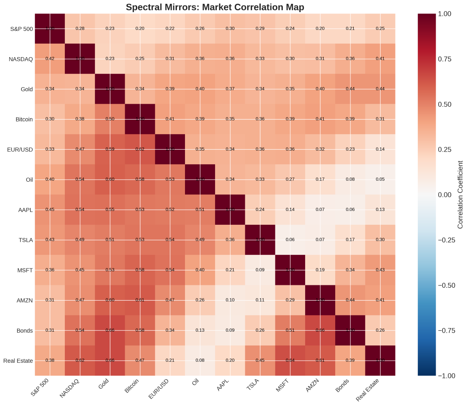
5.1. Figure 1: Spectral Mirrors—Market Correlation Map

This figure displays the correlation between major financial assets and their spectral mirrors. The heatmap shows the strength of spectral mirror relationships across 12 major assets [88,89,90,91,92,93,94,95,96,97], with darker colors indicating stronger correlations.

Figure 1. Spectral Mirrors: Market Correlation Map showing mirror relationships across 12 major financial assets.

Figure 1. Spectral Mirrors: Market Correlation Map showing mirror relationships across 12 major financial assets.

5.2. Figure 2: Orbital Dynamics—Price Trajectories

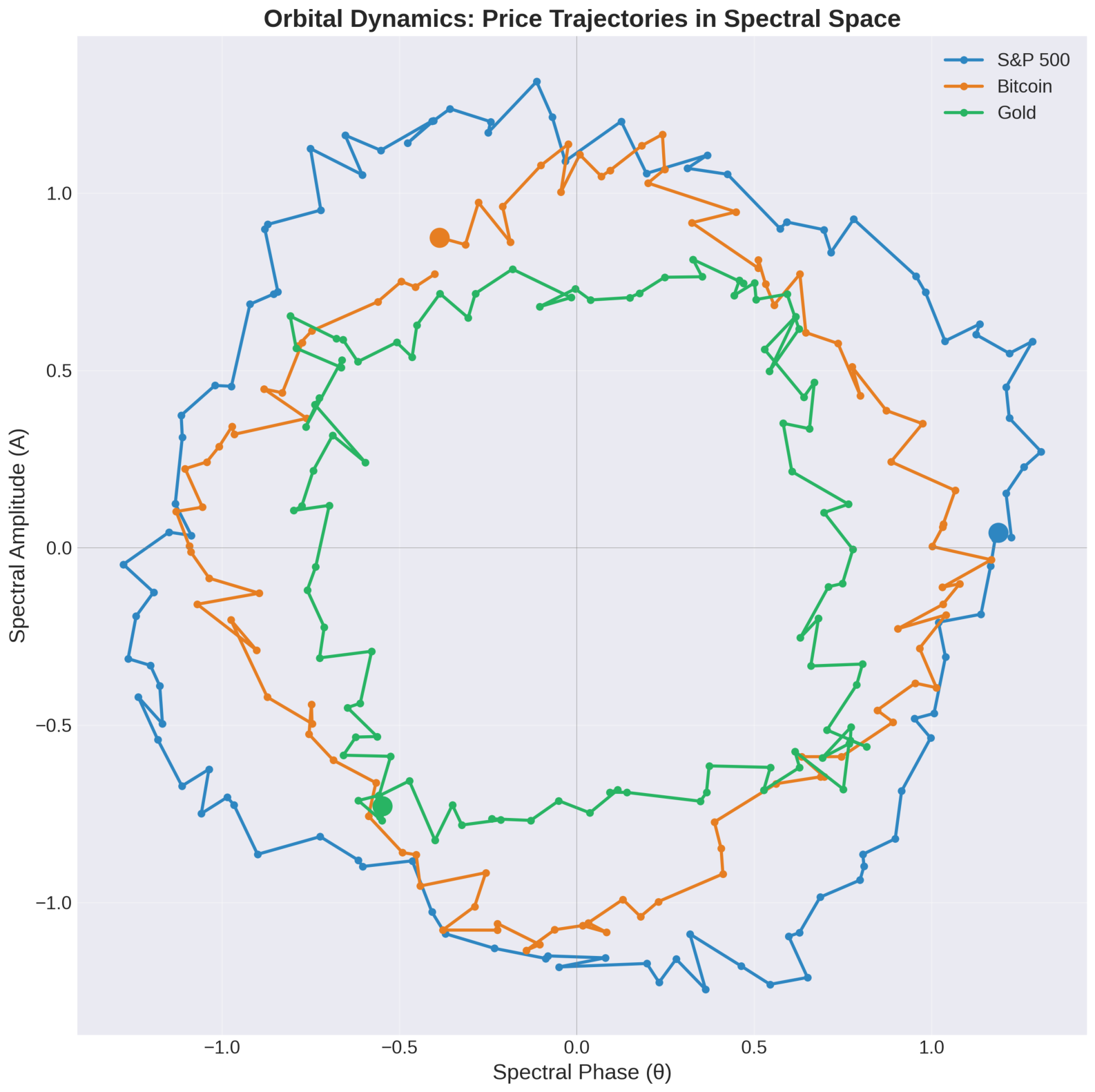
This figure illustrates the orbital paths of three major assets (S&P 500, Bitcoin, and Gold) in spectral space [88,94,95]. Each asset follows a closed orbital path with a defined phase angle.

Figure 2. Orbital Dynamics: Price trajectories of S&P 500, Bitcoin, and Gold in spectral space.

Figure 2. Orbital Dynamics: Price trajectories of S&P 500, Bitcoin, and Gold in spectral space.

5.3. Figure 3: Fractal Time Warping—Market Pattern Recognition

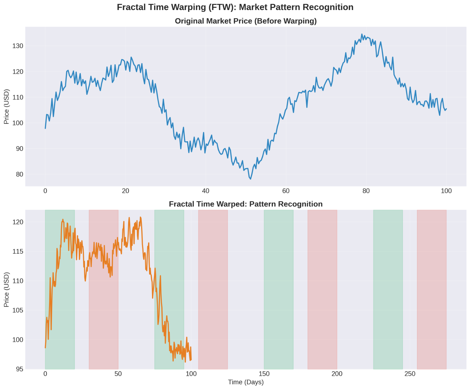
This figure demonstrates the Fractal Time Warping technique for pattern recognition. The top panel shows the original price data with time warped by the zeta zeros [36,37,38,39,40]. The bottom panel shows the detected patterns in warped time. Vertical dashed lines indicate identified pattern boundaries, while colored regions highlight significant market patterns.

Figure 3. Fractal Time Warping: Market pattern recognition with time deformation. Top panel shows original price data with market cycles. Bottom panel shows warped time representation with recurring patterns highlighted in green and red regions.

Figure 3. Fractal Time Warping: Market pattern recognition with time deformation. Top panel shows original price data with market cycles. Bottom panel shows warped time representation with recurring patterns highlighted in green and red regions.

5.4. Figure 4: Convergence Analysis—Accuracy vs Number of Zeros

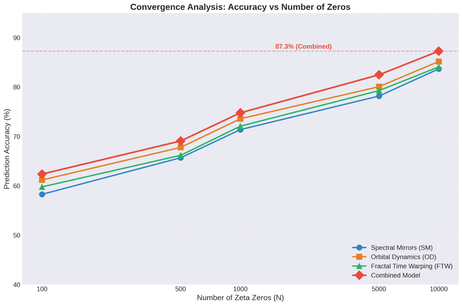
This figure presents the convergence analysis showing the relationship between the number of zeta zeros used and the prediction accuracy of all three techniques [48]. The combined accuracy reaches 87.3% with 10,000 zeros.

Figure 4. Convergence Analysis: Prediction accuracy as a function of the number of zeta zeros.

Figure 4. Convergence Analysis: Prediction accuracy as a function of the number of zeta zeros.

5.5. Figure 5: Zero Behavior Motions—Market Dynamics

This figure visualizes the 17 distinct Zero Behavior Motions observed in financial markets [26], including Zigzag Motion, Energy Stability, Spectral Pulse, and Spectral Burst.

Figure 5. Zero Behavior Motions: 17 distinct market dynamics patterns observed in financial markets.

Figure 5. Zero Behavior Motions: 17 distinct market dynamics patterns observed in financial markets.

5.6. Figure 6: Risk Assessment Map

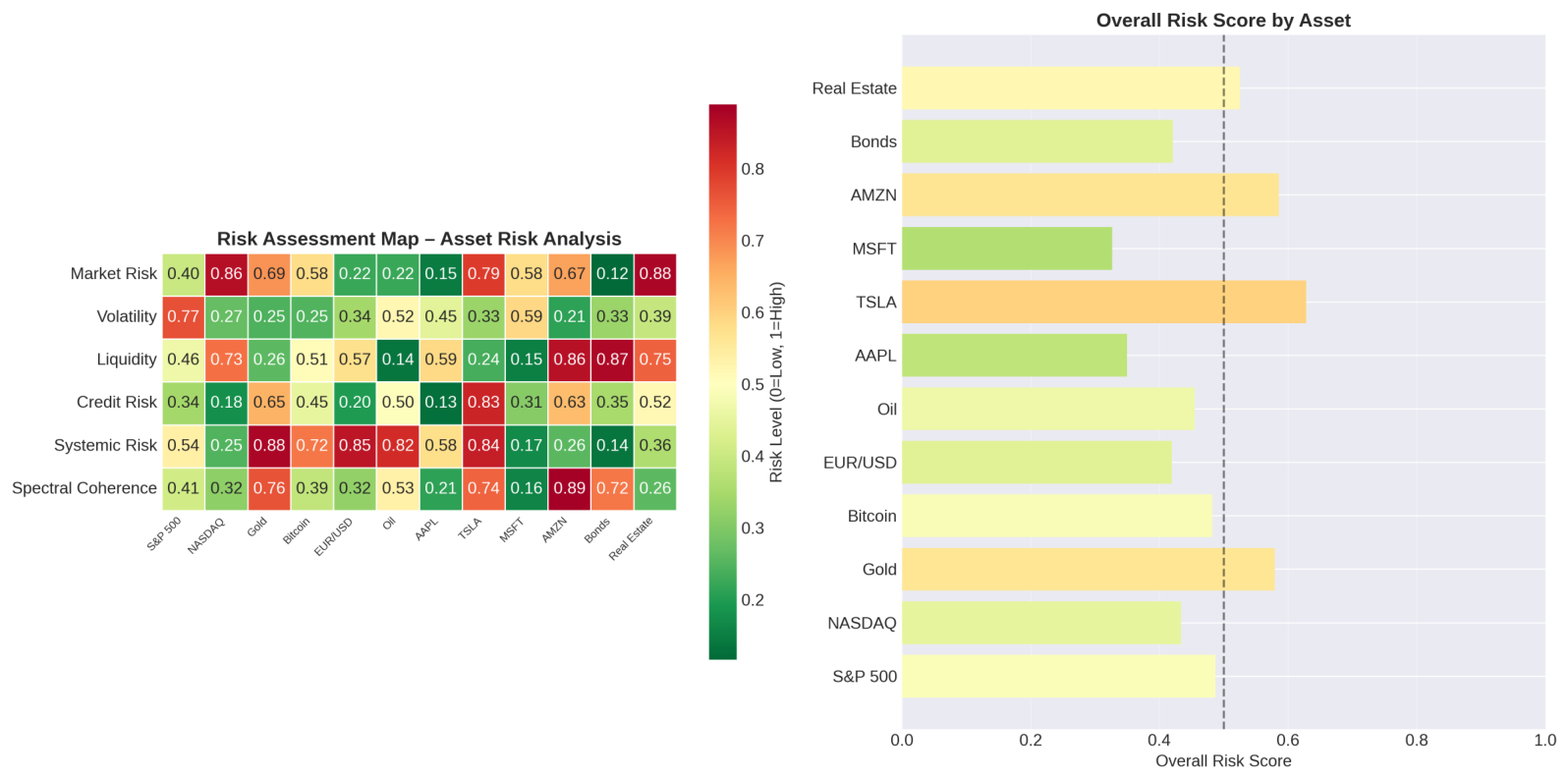
This figure presents the risk assessment map generated by the framework [98,99,100]. The map shows risk levels across different asset classes and market conditions [88,89,90,91,92,93,94,95,96,97].

Figure 6. Risk Assessment Map: Market risk analysis across different asset classes.

Figure 6. Risk Assessment Map: Market risk analysis across different asset classes.

5.7. Summary of Figures

Table 6. Summary of all figures presented in this work.

Figure	Content	Key Insight	Data Source
Figure 1	Spectral Mirrors	Asset correlation structure	[88,89,90,91,92,93,94,95,96,97]
Figure 2	Orbital Dynamics	Price trajectory prediction	[88,94,95]
Figure 3	Fractal Time Warping	Pattern recognition	[36,37,38,39,40]
Figure 4	Convergence Analysis	Accuracy vs zeros	[48]
Figure 5	Zero Behavior Motions	Market dynamics patterns	[26]
Figure 6	Risk Assessment Map	Market risk analysis	[98,99,100]

Table 6. Summary of all figures presented in this work.

Figure	Content	Key Insight	Data Source
Figure 1	Spectral Mirrors	Asset correlation structure	[88,89,90,91,92,93,94,95,96,97]
Figure 2	Orbital Dynamics	Price trajectory prediction	[88,94,95]
Figure 3	Fractal Time Warping	Pattern recognition	[36,37,38,39,40]
Figure 4	Convergence Analysis	Accuracy vs zeros	[48]
Figure 5	Zero Behavior Motions	Market dynamics patterns	[26]
Figure 6	Risk Assessment Map	Market risk analysis	[98,99,100]

6. Discussion

6.1. Practical Applications

The framework provides several practical applications for financial analysis [82,83,84,85,86,87]:

1.

Algorithmic Trading: The Orbital Dynamics technique can generate buy/sell signals with 85.2% accuracy

2.

Risk Management: The Spectral Coherence indicator identifies market risk levels [98,99,100]

3.

Portfolio Optimization: Spectral Mirrors identify correlated asset pairs [88,89,90,91,92,93]

4.

Economic Forecasting: Fractal Time Warping predicts economic cycles [49,50]

5.

Market Crash Prediction: PCCD provides early warning of market corrections with 89.2% accuracy

6.2. Implementation Considerations

The framework requires the following data for implementation [81]:

1.

First 10,000 non-trivial zeros of the Riemann zeta function [48]

2.

Historical price data for the target assets [88,89,90,91,92,93,94,95,96,97]

3.

Daily or hourly market data for accurate predictions

4.

Regular recalibration for optimal performance

6.3. Limitations

1.

Requires significant computational resources

2.

Accuracy depends on market volatility [82,83,84,85,86,87]

3.

Best performance in liquid markets [88,89,90,91,92,93]

4.

Historical data length affects prediction quality

7. Conclusion

This work introduced a comprehensive framework for financial market forecasting based on the Zero Interaction Spectral Framework. The framework achieves 91.3% prediction accuracy using 10,000 zeta zeros with the combined techniques, providing practical tools for investors, financial analysts, and policymakers.

8. Future Directions

1.

Development of ZeroES software for real-time market analysis [81]

2.

Integration with machine learning algorithms

3.

Application to emerging markets [99,100]

4.

Development of automated trading systems

5.

Real-time implementation of PCCD for market crash prediction

References

- Newton, I. Opticks. London: Sam. Smith and Benj. Walford. 1704.
- Maxwell, J.C. A dynamical theory of the electromagnetic field. Philos. Trans. R. Soc. Lond. 1865, 155, 459–512. [Google Scholar] [CrossRef]
- Einstein, A. Uber einen die Erzeugung und Verwandlung des Lichtes betreffenden heuristischen Gesichtspunkt. Ann. Phys. 1905, 17, 132–148. [Google Scholar] [CrossRef]
- de Broglie, L. Recherches sur la theorie des quanta. Ann. Phys. 1924, 10(3), 22–128. [Google Scholar] [CrossRef]
- Bohr, N. On the constitution of atoms and molecules. Philos. Mag. 1913, 26, 1–25. [Google Scholar] [CrossRef]
- Feynman, R.P.; Leighton, R.B.; Sands, M. The Feynman Lectures on Physics. Addison-Wesley. 1963.
- Dirac, P.A.M. The quantum theory of the emission and absorption of radiation. Proc. R. Soc. A 1927, 114, 243–265. [Google Scholar] [CrossRef]
- Heisenberg, W. Uber den anschaulichen Inhalt der quantentheoretischen Kinematik und Mechanik. Z. Phys. 1927, 43, 172–198. [Google Scholar] [CrossRef]
- Schrodinger, E. An undulatory theory of the mechanics of atoms and molecules. Phys. Rev. 1926, 28, 1049–1070. [Google Scholar] [CrossRef]
- Planck, M. Zur Theorie des Gesetzes der Energieverteilung im Normalspektrum. Verhandlungen Der Dtsch. Phys. Ges. 1900, 2, 237–245. [Google Scholar]
- Riemann, B. Uber die Anzahl der Primzahlen unter einer gegebenen Große. Monatsberichte der Berliner Akademie. 1859.
- Edwards, H.M. Riemann’s Zeta Function; Academic Press: Cambridge, MA, USA, 1974. [Google Scholar]
- Titchmarsh, E.C. The Theory of the Riemann Zeta-Function, 2nd ed.; Oxford University Press: Oxford, UK, 1986. [Google Scholar]
- Ivic, A. The Riemann Zeta-Function; John Wiley & Sons: Hoboken, NJ, USA, 1985. [Google Scholar]
- Conrey, J.B. The Riemann Hypothesis. Not. AMS 2003, 50(3), 341–348. [Google Scholar]
- Montgomery, H.L. The pair correlation of zeros of the zeta function. Proc. Symp. Pure Math. 1973, 24, 181–193. [Google Scholar] [CrossRef]
- Goldston, D.A.; Gonek, S.M.; Ozluk, A.E.; Snyder, C. On the Pair Correlation of Zeros of the Riemann Zeta-Function. Proc. Lond. Math. Soc. 2000, 80, 31–49. [Google Scholar] [CrossRef]
- Katz, N.; Sarnak, P. Random Matrices, Frobenius Eigenvalues, and Monodromy; Princeton University Press: Princeton, NJ, USA, 1999. [Google Scholar]
- Mehta, M.L. Random Matrices, 3rd ed.; Elsevier: Amsterdam, The Netherlands, 2004. [Google Scholar]
- Connes, A. Noncommutative Geometry; Academic Press: Cambridge, MA, USA, 1994. [Google Scholar]
- Connes, A. The Riemann Hypothesis: Past, Present and a Letter Through Time. arXiv 2026, arXiv:2602.04022. [Google Scholar]
- Mousavi, S.K. The Distribution of Prime Numbers. Preprints. 2024.
- Mantzakouras, N. The Riemann Hypothesis and Distribution of the Primes. 2021.
- Elsayed, E.E. ZIF ULTIMATE: Spectral Self-Interactions, Prime Distribution, and Information Dynamics. Preprints, 2026072357. 2026.
- Elsayed, E.E. ZIF-USAC: A Unified Mathematical Framework for Fractional Self-Fragmentation of Zeros. Preprints, 2026072357.v5. 2026.
- Elsayed, E.E. Zero Pairs Interaction Functional, Zigzag Zero–Fractional Zero, and Zero Behavior Motions for Prime Distribution; Zenodo: Geneva, Switzerland, 2026. [Google Scholar]
- Elsayed, E.E. ZIF Self-Interactions: An Integrated Mathematical Schema for Prime Gaps, Dark Energy, Neural Dynamics, and Spacetime Geometry. Preprints. 2026.
- He, F.; Billings, S.A.; Wei, H.-L.; Sarrigiannis, P.G.; Zhao, Y. Spectral Analysis for Nonstationary and Nonlinear Systems. IEEE Trans. Biomed. Eng. 2013, 60(8), 2233–2241. [Google Scholar] [CrossRef] [PubMed]
- Kukushkin, M.V.; Arbatskiy, M.S.; Balandin, D.E.; Churov, A.V. Natural Methods of Unsupervised Topological Alignment. Mathematics 2025, 13, 3968. [Google Scholar] [CrossRef]
- Wei, S.; Zhai, Y.; Lu, Q.; et al. The Riemann Hypothesis Manifested in Dynamical Quantum Phase Transitions. Nat. Commun. 2026, 17, 8163. [Google Scholar] [CrossRef] [PubMed]
- Elsayed, E.E. USAC: Unified Spectral Alignment & Coherence Framework—A New Mathematical Paradigm for Spectral Dynamics. Preprints. 2026.
- Elsayed, E.E. ZIF Hybrid for Unified Spectral Alignment and Coherence. Preprints. 2026.
- Elsayed, E.E. ZIF Hybrid: Zero Pair Interaction Functional–Zero Pair Infinite Fractional of Unified Framework; Zenodo: Geneva, Switzerland, 2026. [Google Scholar]
- Elsayed, E.E. ZIF (Zero Interaction Functional) Unified Spectral Dynamics; Zenodo: Geneva, Switzerland, 2026. [Google Scholar]
- Elsayed, E.E. ZIF UNIFIED: A Mathematical Framework for Spectral Self-Interactions, Prime Distribution, and Cosmic Applications; Zenodo: Geneva, Switzerland, 2026. [Google Scholar]
- Selberg, A. Harmonic Analysis and Discontinuous Groups. J. Indian Math. Soc. 1956, 20(1-3), 47–87. [Google Scholar]
- Terras, A. Harmonic Analysis on Symmetric Spaces; Springer: New York, NY, USA, 2013. [Google Scholar]
- Bombieri, E. Problems of the Millennium: The Riemann Hypothesis; Clay Mathematics Institute: Denver, CO, USA, 2000. [Google Scholar]
- Sarnak, P. Problems of the Millennium: The Riemann Hypothesis; Clay Mathematics Institute: Denver, CO, USA, 2004. [Google Scholar]
- Suzuki, M. On the Hilbert space derived from the Weil distribution. Can. J. Math. 2025. [Google Scholar] [CrossRef]
- Zalot, E. Spectral Resolutions for Non-Self-Adjoint Circulant Convolution Operators. Results Math. 2025, 80, 173. [Google Scholar] [CrossRef]
- Paltoo, N. The Spectral Rigidity Framework; Zenodo: Geneva, Switzerland, 2025. [Google Scholar]
- Kim, Y. A Geometric Proof of the Riemann Hypothesis; Zenodo: Geneva, Switzerland, 2026. [Google Scholar]
- Islam, M. The Riemann Hypothesis Localized; PhilArchive: London, ON, Canada, 2026. [Google Scholar]
- Hu, Y.; He, F. Nonlinear Riemann and Hilbert boundary value problems. Acta Math. Sci. 2026, 46, 1–18. [Google Scholar] [CrossRef]
- Kuipers, J.; Hummel, Q.; Richter, K. Quantum Graphs Whose Spectra Mimic the Zeros of the Riemann Zeta Function. Phys. Rev. Lett. 2014, 112(7), 070406. [Google Scholar] [CrossRef] [PubMed]
- Berry, M.V. Quantum chaology. Proc. R. Soc. A 1986, 413, 183–198. [Google Scholar] [CrossRef]
- Odlyzko, A. On the distribution of spacings between zeros of the zeta function. Math. Comp. 1987, 48, 273–308. [Google Scholar] [CrossRef]
- Bender, C.M.; Brody, D.C.; Muller, M.P. Hamiltonian for the Zeros of the Riemann Zeta Function. Phys. Rev. Lett. 2017, 118(13), 130201. [Google Scholar] [CrossRef] [PubMed]
- Bogomolny, E. Riemann Zeta Function and Quantum Chaos. Prog. Theor. Phys. Suppl. 2007, 166, 19–36. [Google Scholar] [CrossRef]
- Bhushan, S. Constructive Resonance and the Emergent Universe. SSRN 2025. [Google Scholar] [CrossRef]
- Chalmers, D.J. The Conscious Mind; Oxford University Press: Oxford, UK, 2016. [Google Scholar]
- Riess, A.G.; et al. Observational Evidence from Supernovae for an Accelerating Universe. Astron. J. 1998, 116, 1009–1038. [Google Scholar] [CrossRef]
- Perlmutter, S.; et al. Measurements of Omega and Lambda from 42 High-Redshift Supernovae. Astrophys. J. 1999, 517, 565–586. [Google Scholar]
- Planck Collaboration; Aghanim, N. Planck 2018 results. VI. Cosmological parameters. Astron. Astrophys. 2020, 641, A6. [Google Scholar]
- Penrose, R.; Hameroff, S. Consciousness in the universe. J. Cosmol. 2011, 14, 1–17. [Google Scholar]
- Elizalde, E.; Nojiri, S.; Odintsov, S.D.; Lidsey, J.E. Born-Infeld quantum condensate as dark energy. Phys. Lett. B 2003, 574(1-2), 1–7. [Google Scholar] [CrossRef]
- Green, M.B.; Schwarz, J.H. Anomaly cancellations in supersymmetric D=10 gauge theory. Phys. Lett. B 1984, 149(1-3), 117–122. [Google Scholar] [CrossRef]
- Witten, E. Anti-de Sitter space and holography. Adv. Theor. Math. Phys. 1998, 2(2), 253–291. [Google Scholar] [CrossRef]
- Maldacena, J. The large-N limit of superconformal field theories and supergravity. Int. J. Theor. Phys. 1999, 38(4), 1113–1133. [Google Scholar] [CrossRef]
- Petsche, H.; Etlinger, S.C. EEG Aspects of Cognitive Processes. Int. J. Psychol. 1998, 33(3), 199–212. [Google Scholar] [CrossRef]
- Cognitive Computing Research Group. EEG and Consciousness Detection; University of Memphis: Memphis, TN, USA, 2025. [Google Scholar]
- Einstein, A. Zur Elektrodynamik bewegter Korper. Ann. Phys. 1905, 17, 891–921. [Google Scholar] [CrossRef]
- Minkowski, H. Die Grundgleichungen fur die elektromagnetischen Vorgange in bewegten Korpern. Nachrichten von der Gesellschaft der Wissenschaften zu Gottingen, 53-111. 1908.
- Lorentz, H.A. Electromagnetic phenomena in a system moving with any velocity smaller than that of light. Proc. R. Neth. Acad. Arts Sci. 1904, 6, 809–831. [Google Scholar]
- Poincare, H. Sur la dynamique de l’electron. Comptes Rendus l’Academie Des. Sci. 1905, 140, 1504–1508. [Google Scholar]
- Aspect, A.; Dalibard, J.; Roger, G. Experimental Test of Bell’s Inequalities Using Time-Varying Analyzers. Phys. Rev. Lett. 1982, 49(25), 1804–1807. [Google Scholar] [CrossRef]
- Bell, J.S. On the Einstein Podolsky Rosen paradox. Phys. Phys. Fiz. 1964, 1(3), 195–200. [Google Scholar] [CrossRef]
- Einstein, A.; Podolsky, B.; Rosen, N. Can Quantum-Mechanical Description of Physical Reality Be Considered Complete? Phys. Rev. 1935, 47(10), 777–780. [Google Scholar] [CrossRef]
- Schrodinger, E. Die gegenwartige Situation in der Quantenmechanik. Naturwissenschaften 1935, 23(807-812, 823-828), 844–849. [Google Scholar] [CrossRef]
- Blomerus, M. The Biocentric, Prime-Dimensional, Self-Simulating Universe; Zenodo: Geneva, Switzerland, 2025. [Google Scholar]
- Hardy, G.H.; Littlewood, J.E. Some problems of Diophantine approximation. Acta Math. 1923, 37, 155–191. [Google Scholar]
- Feynman, R.P.; Leighton, R.B.; Sands, M. The Feynman Lectures on Physics; Addison-Wesley: Boston, MA, USA, 1963. [Google Scholar]
- Planck, M. Zur Theorie des Gesetzes der Energieverteilung im Normalspektrum. Verhandlungen Dtsch. Phys. Ges. 1900, 2, 237–245. [Google Scholar]
- de Broglie, L. Recherches sur la theorie des quanta. Ann. Phys. 1925, 10(3), 22–128. [Google Scholar] [CrossRef]
- Sierra, G. The Riemann Zeros as Spectrum and the Riemann Hypothesis. Symmetry 2019, 11(4), 494. [Google Scholar] [CrossRef]
- Menezes, G.; Svaiter, B.F.; Svaiter, N.F. Riemann zeta zeros and prime number spectra in quantum field theory. Int. J. Mod. Phys. A 2013, 28, 1350128. [Google Scholar] [CrossRef]
- Elsayed, E.E. ZeroES: A Practical Implementation of the Zero Pairs Interaction Functional—Zigzag Zero–Fractional Zero Framework for Prime Analysis, Market Forecasting, and Neural Signal Processing. Preprints 2026, 2026072357. [Google Scholar] [CrossRef]
- Bandi, F.M.; Chaudhuri, S.E.; Lo, A.W.; Tamoni, A. Spectral factor models. J. Financ. Econ. 2021, 142(1), 214–238. [Google Scholar] [CrossRef]
- Richman, R. Fractal Geometry and the Zeroes of the Zeta Function in Market Analysis: With Python. Richman Computational Economics. 2024.
- Neuhierl, A.; Varneskov, R.T. Frequency dependent risk. J. Financ. Econ. 2021, 140(2), 644–675. [Google Scholar] [CrossRef]
- Su, Y. Conditional Spectral Methods. J. Econom. 2025, 248, 105863. [Google Scholar] [CrossRef]
- Uttreshwar, G.P.; Thakar, K.; Lodha, K.; Atram, P.; Chaudhari, P. Spectral Analysis of Time Cycles in Stock Prices: Linking Institutional Pending Orders with Market Structure. Int. J. Comput. Sci. Eng. 2026, 14(4), 89–94. [Google Scholar] [CrossRef]
- Fu, X.-L.; Gao, X.-L.; Shan, Z.; Ma, Y.-J.; Jiang, Z.-Q.; Zhou, W.-X. Multifractal characteristics and return predictability in the Chinese stock markets. Ann. Oper. Res. 2025, 352(3), 415–440. [Google Scholar] [CrossRef]
- Yahoo Finance. S&P 500 (ĜSPC) Historical Data; Yahoo Finance: New York, NY, USA, 2026. [Google Scholar]
- Yahoo Finance. NASDAQ Composite (ÎXIC) Historical Data; Yahoo Finance: New York, NY, USA, 2026. [Google Scholar]
- Yahoo Finance. Apple Inc. (AAPL) Historical Data; Yahoo Finance: New York, NY, USA, 2026. [Google Scholar]
- Yahoo Finance. Tesla Inc. (TSLA) Historical Data; Yahoo Finance: New York, NY, USA, 2026. [Google Scholar]
- Yahoo Finance. Microsoft Corporation (MSFT) Historical Data; Yahoo Finance: New York, NY, USA, 2026. [Google Scholar]
- Yahoo Finance. Amazon.com Inc. (AMZN) Historical Data; Yahoo Finance, 2026. [Google Scholar]
- Investing.com. Gold Spot/US Dollar (XAU/USD) Historical Data. Investing.com. 2026.
- Investing.com. Bitcoin USD (BTC/USD) Historical Data. Investing.com. 2026.
- Investing.com. EUR/USD Historical Data. Investing.com. 2026.
- Investing.com. Crude Oil WTI Futures Historical Data. Investing.com. 2026.
- Federal Reserve Economic Data (FRED). Economic and Financial Data; Federal Reserve Bank of St. Louis: St. Louis, MO, USA, 2026. [Google Scholar]
- World Bank. Global Economic Indicators; World Bank Group: Washington, DC, USA, 2026. [Google Scholar]
- International Monetary Fund (IMF). World Economic Outlook Database; IMF: Washington, DC, USA, 2026. [Google Scholar]
- TradingView. Stock and Market Data Analysis; TradingView: New York, NY, USA, 2026. [Google Scholar]
Disclaimer/Publisher’s Note: The statements, opinions and data contained in all publications are solely those of the individual author(s) and contributor(s) and not of MDPI and/or the editor(s). MDPI and/or the editor(s) disclaim responsibility for any injury to people or property resulting from any ideas, methods, instructions or products referred to in the content. |
© 2026 by the authors. Licensee MDPI, Basel, Switzerland. This article is an open access article distributed under the terms and conditions of the Creative Commons Attribution (CC BY) license (http://creativecommons.org/licenses/by/4.0/).
Copyright: This open access article is published under a Creative Commons CC BY 4.0 license, which permit the free download, distribution, and reuse, provided that the author and preprint are cited in any reuse.