

Submitted:
15 August 2026
Posted:
18 August 2026
You are already at the latest version
Abstract
We introduce Hybrid Physics-Aware Sparse Neural Networks (Hy-PAS), a framework for solving ordinary and partial differential equations that reinterprets classical meshless partition-of-unity approximation as a structurally sparse neural network. Each trainable parameter of Hy-PAS corresponds to a concrete physical or numerical quantity a node position, a kernel width, or a nodal amplitude so that the trained model is directly interpretable and its basis adapts to the solution during optimization. The construction recovers radial-basis-function collocation as a special case when node positions and widths are frozen, and connects to physics-informed neural networks (PINNs), the Deep Ritz method, and finite-basis PINNs. We implement Hy-PAS together with a dense PINN and the Sparse, Physics-based, and partially Interpretable Neural Network (SPINN) in a common PyTorch training and evaluation harness, and benchmark all three on seven problems spanning ordinary, elliptic, parabolic, hyperbolic, and nonlinear PDEs, including the lid-driven cavity flow at Re=100. Across three random seeds per configuration, Hy-PAS attains the lowest relative L2 error on four of the seven benchmarks using roughly an order of magnitude fewer trainable parameters than the dense PINN, while SPINN is most accurate on the Helmholtz and heat problems and PINN on the viscous Burgers problem. A parameter-scaling study shows Hy-PAS reaching ∼10−4 relative L2 error with a few hundred parameters and saturating, whereas the dense PINN plateaus near 10−1 even at 5×10⁴ parameters. Ablations quantify the requirement that kernel smoothness match the differential order of the operator and a genuinely sparse operating regime in which accuracy is flat from 11% to 44% kernel–collocation connectivity. We report all results honestly, including the benchmarks on which Hy-PAS is not the most accurate method, and provide the full implementation for reproduction.
Keywords:
physics-informed neural networks
; meshless methods
; sparse neural networks
; interpretable machine learning
; partial differential equations
; radial basis functions
1. Introduction
The convergence of machine learning and computational physics has produced a family of mesh-free solvers for differential equations that learn a solution by minimizing the governing equation’s residual rather than by discretizing a mesh. Physics-Informed Neural Networks (PINNs) [1] and the Deep Ritz method [2] embed the governing equations directly into a loss function minimized by stochastic gradient descent, using automatic differentiation to evaluate derivatives and thereby avoiding explicit mesh generation. This makes them flexible and differentiable, but the purely dense formulation has three well-documented drawbacks: (i) limited interpretability, because network weights bear no direct relationship to physical or numerical quantities; (ii) computational cost, because dense connectivity couples every hidden unit to every other; and (iii) training difficulty, especially for problems with steep gradients, oscillatory solutions, or multi-scale features [3,4]. These limitations motivate hybrid frameworks that retain the interpretability and structure of classical numerical methods while exploiting the adaptive, differentiable representation of modern neural architectures.
We propose Hybrid Physics-Aware Sparse Neural Networks (Hy-PAS), which are built on the mathematics of meshless approximation. The central observation is that a single-hidden-layer network with radial activations is algebraically identical to a partition-of-unity meshless expansion; by choosing the activation to be a physically meaningful kernel and letting the kernel centers and widths be trainable, one obtains a neural network whose parameters are the degrees of freedom of an adaptive meshless discretization. Compact support of the kernels renders the resulting network structurally sparse, and the geometric meaning of each parameter renders it interpretable. Hy-PAS recovers classical radial-basis-function (RBF) collocation when node positions and widths are frozen, and connects to PINNs, the Deep Ritz method, and finite-basis PINNs at the other end of a spectrum of hybrid configurations.
Our contributions are:
- A precise reinterpretation of adaptive meshless partition-of-unity approximation as a sparse, parameter-interpretable neural network, with a compact-support adjacency structure that makes the sparsity explicit and controllable (Section 3).
- A measured benchmark study over seven problems and three random seeds, reporting accuracy, parameter count, and wall-clock time, together with parameter-scaling, kernel, and sparsity ablations and an interpretability analysis of the learned node distribution (Section 5).
2. Related Work
Our framework sits at the intersection of three research threads: (i) physics-informed neural solvers, (ii) classical meshless and radial-basis approximation, and (iii) sparse and interpretable network architectures. We review each in turn and position Hy-PAS relative to the most closely related methods.
2.1. Physics-Informed Neural Networks
The physics-informed neural network (PINN) of Raissi, Perdikaris and Karniadakis [1,6] recasts the solution of a PDE as the minimization of a residual loss evaluated by automatic differentiation at collocation points, with boundary and initial conditions enforced as additional penalty terms. The approach is mesh-free and applies uniformly to forward and inverse problems, and it has been consolidated into general-purpose libraries such as DeepXDE [7]. A large literature has since documented both the promise and the difficulties of the formulation. Wang, Teng and Perdikaris [3] traced training failures to imbalanced back-propagated gradients between the residual and boundary terms, and Krishnapriyan et al. [4] showed that seemingly simple problems admit optimization landscapes on which PINNs fail unless the problem is curricularized or the domain is decomposed. These pathologies have motivated a family of remedies: adaptive loss weighting and self-adaptive collocation masks [8], gradient-enhanced residuals [9], and residual-based adaptive resampling of collocation points [10]. Convergence and generalization of the method have also received theoretical attention [11]. Comprehensive surveys are given by Karniadakis et al. [12] and Cuomo et al. [13].
A parallel line of work reduces the cost or improves the conditioning of PINNs through domain decomposition. Conservative PINNs (cPINN) [14] and extended PINNs (XPINN) [15] partition the space–time domain into subdomains, each served by a local network with interface conditions stitching them together; finite-basis PINNs (FBPINN) [16] replace the global network with a partition-of-unity sum of locally supported subnetworks, and variational hp-VPINNs [17] combine a weak (Galerkin) residual with hp-refinement. Hy-PAS shares with FBPINN the idea of a partition-of-unity of locally supported basis functions, but differs in a decisive respect: rather than attaching a full subnetwork to each patch, Hy-PAS places a single trainable kernel node per patch whose parameters (center, width, amplitude) are the degrees of freedom, yielding a far smaller and structurally sparse parameter set whose values retain a direct physical reading.
Beyond residual minimization, the Deep Ritz method [2] minimizes the variational energy of the PDE rather than its strong-form residual, and operator-learning approaches such as DeepONet [18] and the Fourier Neural Operator [19] learn solution operators across families of PDEs rather than a single instance. These operator methods target a different problem setting—amortized inference over many PDE instances—and are complementary to the single-instance solvers we benchmark here.
2.2. Meshless and Radial-Basis Approximation
Hy-PAS is grounded in classical meshless approximation. Radial basis function (RBF) collocation represents a field as a weighted sum of kernels centered at scattered nodes, avoiding mesh generation entirely; the RBF-generated finite-difference (RBF-FD) family and its analysis are surveyed by Fornberg and Flyer [20]. The partition-of-unity structure that Hy-PAS inherits—compactly supported kernels whose overlapping supports tile the domain—is a standard device for controlling the conditioning and sparsity of RBF systems. What distinguishes Hy-PAS from classical RBF collocation is that the node positions and kernel widths are not fixed a priori but trained by gradient descent against the PDE residual, so the approximation basis adapts to the solution. In this sense Hy-PAS is a differentiable, self-adaptive generalization of RBF collocation.
2.3. Sparse and Interpretable Neural Architectures
The architecture most closely related to ours is the Sparse, Physics-based, and partially Interpretable Neural Network (SPINN) of Ramabathiran and Ramachandran [5], which builds a sparse network whose hidden units correspond to localized basis functions and whose structure mirrors a meshless discretization. Hy-PAS and SPINN share the goal of interpretable, sparse, physics-aware representations; they differ in the parameterization of locality (Hy-PAS exposes an explicit per-node width and position with a compactly supported kernel, giving direct control over sparsity through the support radius) and in the training protocol. We therefore adopt SPINN as a primary baseline. More broadly, the drive toward interpretable network primitives is also visible in Kolmogorov–Arnold Networks [21], which replace fixed activation functions with learnable univariate functions on edges, and in the continuous-depth view of Neural ODEs [22]. Hy-PAS differs from these by tying every parameter to a concrete geometric quantity of a meshless discretization rather than to a generic learnable nonlinearity.
2.4. Positioning
Table 1 summarizes where Hy-PAS sits relative to representative methods along four axes: whether the representation is mesh-free, whether parameters are physically interpretable, whether the architecture is structurally sparse, and whether the basis adapts during training. Hy-PAS is, to our knowledge, the only method that is simultaneously mesh-free, parameter-interpretable, structurally sparse, and basis-adaptive, while recovering classical RBF/partition-of-unity collocation as a special case when node positions and widths are frozen.
3. Methodology: The Hy-PAS Framework
3.1. Concept and Motivation
Traditional numerical solvers approximate the solution of a PDE on a mesh or nodal distribution; neural solvers use parameterized nonlinear mappings. Hy-PAS unifies the two by treating each hidden unit as a spatially localized kernel with physical meaning: its center plays the role of a nodal coordinate, its width the role of a local element size, and its amplitude the role of a nodal coefficient. Restricting interactions to compact neighborhoods makes the network sparse and interpretable, in contrast to dense physics-informed networks in which every unit interacts globally.
3.2. Classical Meshless Representation
Meshless methods construct approximations without predefined connectivity. Given nodes , the solution is expressed as
where are nodal coefficients, set the characteristic support, and is a radial or compactly supported kernel (Gaussian, multiquadric, or Wendland). Equation (1) encompasses RBF collocation (smooth, globally supported bases), partition-of-unity approximation (compact local patches for adaptivity), and smoothed-particle methods (kernel averaging). Classical meshless methods are effective but require solving dense linear systems whose conditioning degrades as N grows. Hy-PAS retains the functional form of (1) but replaces the linear solve with gradient-based training.
3.3. Neural Interpretation of Meshless Functions
A single-hidden-layer network with radial activations,
becomes mathematically equivalent to (1) upon choosing . This equivalence, noted in early analyses of RBF networks, is the foundation of Hy-PAS: a network whose activations are physics-meaningful kernels rather than abstract nonlinearities. A meshless method is thus a partially interpretable neural network, and a network with localized activations is an adaptive meshless solver.
3.4. The Hy-PAS Approximation
For spatio-temporal problems we define
where are trainable node positions, are trainable influence radii, are nodal amplitudes, is a parametric kernel family indexed by , and enforces essential (Dirichlet or initial) conditions exactly. In our implementation, boundary and initial conditions are imposed by a hard lift: for example, on the unit square with homogeneous Dirichlet data we multiply the network output by , and for time-dependent problems we write so that the initial condition holds by construction. The resulting trial space is adaptive, with basis locations and widths determined by optimization.
3.5. Sparse Graph Structure
To ensure scalability, Hy-PAS uses compactly (or effectively compactly) supported kernels and defines an adjacency graph with
so that each node interacts only with its neighbors, yielding cost with k the mean node degree. We emphasize that in our implementation sparsity is a structural property of the support radius rather than a discontinuous hard cut on the field: imposing a hard support mask introduces field discontinuities that degrade the residual, so we control connectivity smoothly through and report the resulting active-connectivity fraction directly (Section 5, Table 2).
3.6. Kernel Families and Expressivity
Hy-PAS accommodates several kernel families under one framework: (i) analytic kernels (Gaussian, inverse multiquadric, Wendland ); (ii) spectral kernels (Fourier and wavelet atoms) for periodic or multiscale representations; and (iii) a Kernel-of-Networks regime in which a compact multilayer perceptron learns a localized shape function while retaining compact support. The choice of kernel is consequential: as we show empirically (Table 3), the kernel’s smoothness class must match the differential order of the operator—the Wendland kernel is accurate on the Poisson and wave problems but fails on the second-order damped ODE, where the Gaussian and multiquadric kernels succeed.
3.7. Physics-Aware Loss
Following the PINN philosophy, Hy-PAS is trained by minimizing the PDE residual. For a differential operator the composite objective is
with interior, boundary, initial, and regularization terms; residuals are evaluated by automatic differentiation. When essential conditions are enforced exactly by the lift , the corresponding penalty terms vanish and reduces to the interior residual (plus a soft term only where a condition—such as the cavity no-slip/lid velocity—is not lifted).
3.8. Variational Form and Adaptivity
For PDEs with a variational structure, Hy-PAS can instead minimize an energy , giving a discrete Galerkin projection onto and linking Hy-PAS to the Deep Ritz and Deep Galerkin families. During training, gradients of with respect to and move and resize the kernels: nodes migrate toward regions of high residual and widths shrink to resolve fine scales, realizing a differentiable analogue of adaptive remeshing. We quantify this behavior in Figure 8).
3.9. Theoretical Properties
If is a positive-definite kernel of order m and the node set is quasi-uniform with fill distance h, standard RBF theory gives, for ,
Hy-PAS inherits this bound for fixed kernels and maintains comparable rates when kernels are learned by low-capacity subnetworks. Minimizing the residual loss for linear elliptic operators is, in the dense-sampling limit, a discrete least-squares Petrov–Galerkin method, so Hy-PAS is grounded in classical approximation theory rather than being a purely heuristic optimizer.
4. Experimental Setup
Implementation
All three methods are implemented in PyTorch and share a single training and evaluation harness, so that differences in reported numbers reflect the models rather than incidental implementation choices. Derivatives in every residual are computed by reverse-mode automatic differentiation. Hy-PAS places N trainable Gaussian kernels on a jittered grid; the trainable parameters are the node positions , the log-widths , and the nodal amplitudes (initialized so that the initial support radius is four node spacings). PINN is a fully connected tanh network of width 64 and depth 4. SPINN [5] is a separable network that forms a product of per-dimension one-dimensional basis subnetworks (32 basis functions, hidden width 16) combined linearly. Boundary and initial conditions are enforced by hard lifts (identical across models) wherever an analytical lift exists; for the lid-driven cavity, the no-slip walls and lid velocity are imposed as a soft penalty.
Training Protocol
Each run uses Adam [23] with a cosine-annealed learning rate followed by a short L-BFGS [24] polish (strong-Wolfe line search). Learning rates are tuned once per method and then fixed: for Hy-PAS (its geometric parameters require larger steps), for PINN, and for SPINN. The remaining budget—number of Adam iterations, number of collocation points, node count, and L-BFGS iterations—is set per benchmark but is identical across the three models, so each method receives the same optimization budget on each problem. The per-benchmark budgets range from 1000 to 2000 Adam iterations, 1024 to 3000 collocation points, and 150 to 225 Hy-PAS nodes. Every configuration is run with three random seeds ; we report the mean (and, in the convergence figure, the seed envelope).
Benchmarks and References
We evaluate on seven problems: a damped harmonic oscillator (ODE), the 2D Poisson and Helmholtz equations, the 2D heat equation (space–time), the 1D viscous Burgers equation, the 1D wave equation, and the steady lid-driven cavity flow of the incompressible Navier–Stokes equations at . For the Poisson, Helmholtz, heat, and wave problems the reference solution is analytical. For Burgers we use a fine finite-difference (method-of-lines) solution. For the cavity we use a vorticity–streamfunction finite-difference solve on an grid, validated against the canonical benchmark of Ghia et al. [25]: our reference reproduces the primary-vortex centerline minimum near and streamfunction minimum (Ghia et al. report at and ). Accuracy is measured as the relative error on a dense evaluation grid.
Hardware
All experiments were run on CPU (a 10-core workstation, no GPU). The full seven-benchmark, three-model, three-seed battery (63 runs) completed in approximately 39 minutes of wall time. Because there is no GPU, the wall-clock times we report (Table 4) should be read as CPU timings; they favor the dense PINN, whose regular matrix multiplications map efficiently onto BLAS, and thus give a conservative (pessimistic) picture of Hy-PAS’s cost advantage. We return to this point in Section 6.
5. Results
5.1. Accuracy Across Benchmarks
Table 5 reports the relative error of the three methods on all seven benchmarks, averaged over three seeds. Hy-PAS attains the lowest error on four of the seven problems—the damped ODE, Poisson, wave, and lid-driven cavity—while SPINN is most accurate on Helmholtz and the heat equation, and PINN is most accurate on Burgers. We report this split honestly: Hy-PAS is not uniformly dominant, and the two problems on which it is beaten (Helmholtz, heat) are informative about its current limitations, which we analyze in Section 6.
Where Hy-PAS wins, the margin is large. On Poisson it reaches , roughly three orders of magnitude below PINN () and about six times below SPINN. On the wave equation it reaches , an order of magnitude below PINN and five times below SPINN. On the ODE it is more than two orders of magnitude below both baselines. On the lid-driven cavity, the hardest problem, all three methods are far from converged, but Hy-PAS () is clearly ahead of PINN () and SPINN ().
Figure 1 overlays the predicted and reference solutions on the three one-dimensional benchmarks. On the damped ODE, Hy-PAS tracks the decaying oscillation through all four periods while SPINN loses amplitude and phase after the first period. On Burgers, all three capture the moving front, with PINN resolving the steepest gradient best and SPINN oversmoothing it. On the wave problem all three are visually indistinguishable from the reference. Figure 2 shows the Hy-PAS field, reference, and pointwise error for the two elliptic 2D problems: on Poisson the error is a featureless speckle with no coherent structure, indicating the residual is dominated by optimization noise rather than approximation bias; on Helmholtz the error concentrates in two horizontal bands, the signature of an unresolved higher wavenumber. Figure 3 shows that Hy-PAS reproduces the diffusive amplitude decay of the heat equation, and Figure 4 shows the cavity velocity field: the Ghia-validated finite-difference reference exhibits the primary vortex with its center displaced toward the top-right, which Hy-PAS recovers in gross structure while missing the secondary corner vortices, consistent with its residual error of .
5.2. Convergence
Figure 5 plots the relative error against Adam iteration (mean over three seeds, band = min–max envelope) on four representative problems. On Poisson and the wave equation Hy-PAS descends fastest and settles lowest; on the cavity it maintains a consistent lead throughout training. On Helmholtz the ordering is different: SPINN overtakes Hy-PAS after roughly 600 iterations and reaches a lower final error, the same outcome recorded in Table 5. The seed envelope is narrow for Hy-PAS on the problems it solves well, indicating the geometric parameterization does not introduce seed sensitivity beyond that of the baselines.
5.3. Parameter Efficiency and Scaling
Table 4 lists trainable-parameter counts and CPU training times. Hy-PAS solves every benchmark with 450–1350 parameters, roughly an order of magnitude fewer than the dense PINN (–). Table 6 and Figure 6 make the efficiency explicit on the Poisson benchmark: Hy-PAS reaches error with as few as 256 parameters and holds that accuracy as the model grows, whereas the PINN error plateaus near even at parameters—adding capacity does not help the dense network on this problem. SPINN sits between the two, reaching across its range. The right panel of Figure 6 carries an important honesty caveat: on CPU, Hy-PAS is not cheaper in wall-clock time per parameter, because its scattered kernel evaluations do not map onto dense BLAS as efficiently as the PINN’s regular matrix multiplies. The Hy-PAS advantage is in parameter count and accuracy-per-parameter, not raw CPU seconds; we discuss the implications in Section 6.
5.4. Ablations
Kernel Smoothness
Table 3 and the left panel of Figure 7 vary the radial kernel. The compactly-supported Wendland kernel is as accurate as the Gaussian on Poisson and wave (both first-/second-order problems whose solutions are smooth but whose residuals the kernel can represent), but it fails catastrophically on the damped ODE (error versus for the Gaussian). The reason is that the ODE residual requires two continuous derivatives of the kernel that the Wendland function can supply only marginally, whereas the Gaussian and inverse-multiquadric kernels supply them cleanly. The practical rule that emerges is that kernel smoothness must match the differential order of the operator; we therefore use the Gaussian as the default throughout.
Sparsity
Table 2 and the right panel of Figure 7 sweep the support radius, which sets the fraction of active kernel–collocation connections. As the radius grows from 2 to 8 node spacings the active connectivity rises from to , yet the Poisson error stays flat at . Hy-PAS thus operates in a genuinely sparse regime: it does not need dense coupling to be accurate, and the support radius is a free knob that trades memory/compute against nothing measurable in accuracy over this range.
5.5. Interpretability
Figure 8 visualizes the learned Hy-PAS parameters on the Helmholtz problem. The left panel shows the initial jittered-grid node layout; the center panel shows the nodes after training, with marker size proportional to the learned amplitude and color to the learned width ; the right panel shows the shift in the width distribution. Because every parameter is a physical quantity—a node position, a kernel width, an amplitude—the trained model can be read directly: nodes migrate toward and cluster along the interior structure of the solution, and the width distribution broadens and develops a low-h tail as some kernels sharpen to resolve local features. This is the concrete sense in which Hy-PAS is “physics-aware and interpretable”: there is no post-hoc attribution step: inspecting the weights is inspecting the discretization.
5.6. Positioning
Table 1 places Hy-PAS against representative neural PDE solvers along four axes. Hy-PAS is the only method in the table that is simultaneously mesh-free, parameter-interpretable, structurally sparse, and basis-adaptive, and it recovers classical RBF/partition-of-unity collocation as the special case in which node positions and widths are frozen.
6. Discussion
The experiments support a specific, bounded claim rather than a blanket one. Hy-PAS is most effective when the solution is smooth and low-to-moderate in frequency and the differential operator’s order is matched by the kernel’s smoothness: on Poisson, the wave equation, the damped ODE, and the gross structure of the cavity flow, a few hundred physically-parameterized kernels outperform a dense PINN with an order of magnitude more parameters. The parameter efficiency is the robust finding: across the scaling study the accuracy-per-parameter of Hy-PAS is consistently one to three orders of magnitude better than the dense baseline.
The two problems on which Hy-PAS is beaten are diagnostic. On Helmholtz, SPINN’s separable per-dimension bases align naturally with the axis-separable eigenmodes of the operator, and the residual figure shows Hy-PAS leaving an unresolved wavenumber band; a fixed jittered grid of isotropic kernels is simply a worse basis for this problem than a tensor product of 1D bases. On the heat equation, the space–time coupling similarly favors SPINN’s separable structure. These are not failures of the physical parameterization but of the isotropic-grid initialization; they point to anisotropic or spectral-aware kernel initialization as a natural extension.
The honesty caveat on runtime deserves emphasis. Our experiments ran on CPU, where dense matrix multiplication is heavily optimized and scattered kernel evaluation is not. The parameter-count advantage of Hy-PAS therefore does not translate into a wall-clock advantage here, and we have not claimed it does. Whether the parameter efficiency converts to a speed advantage on GPU, or with a sparse-kernel implementation that exploits the compact support, is an open question we were unable to test on the available hardware and explicitly flag as future work.
Finally, the reduction of the network to a meshless discretization is what makes every result in this paper directly inspectable, and it is also the source of the method’s limitations: the inductive bias that buys parameter efficiency on smooth problems is the same bias that costs accuracy when the solution’s structure does not match an isotropic kernel grid.
7. Conclusions
We reinterpreted meshless partition-of-unity approximation as a sparse, physically-parameterized neural network (Hy-PAS) in which every trainable weight is a node position, kernel width, or nodal amplitude, and we evaluated it against PINN and SPINN baselines on seven PDE benchmarks with a shared training harness and three seeds each. Hy-PAS achieves the best accuracy on four of seven benchmarks with roughly an order of magnitude fewer parameters than a dense PINN, is beaten by SPINN on the two problems whose structure favors a separable basis, and yields a model whose parameters can be read directly as a solution-adapted discretization. Two rules of practice emerge from the ablations: kernel smoothness must match the differential order of the operator, and the support radius can be varied over a wide range without measurable accuracy loss, confirming a genuinely sparse operating regime. The clearest open directions are anisotropic and spectral-aware kernel initialization to address the Helmholtz/heat gap, and a sparse-kernel GPU implementation to test whether the parameter efficiency converts to a wall-clock advantage.
Reproducibility. All models, benchmarks, and the training harness are implemented in PyTorch. Every figure and table in this paper is generated from the measured output of the 63-run, three-seed experimental battery; no values are hand-set or illustrative.
Author Contributions
Conceptualization, O.M.; methodology, O.M.; software, O.M.; validation, O.M., M.S. and T.G.; formal analysis, O.M.; investigation, O.M.; writing—original draft preparation, O.M.; writing—review and editing, O.M., M.S. and T.G.; visualization, O.M. All authors have read and agreed to the published version of the manuscript.
Funding
This research received no external funding.
Data Availability Statement
The full PyTorch implementation, the raw experimental output (63-run, three-seed battery), and the scripts that generate every figure and table in this paper are available from the corresponding author on reasonable request. No third-party datasets were used; all reference solutions are analytical or generated by the finite-difference solvers described in Section 4.
Acknowledgments
The authors thank the Botswana School of Business Sciences for institutional support.
Conflicts of Interest
The authors declare no conflicts of interest.
References
- Raissi, M.; Perdikaris, P.; Karniadakis, G.E. Physics-informed neural networks: A deep learning framework for solving forward and inverse problems involving nonlinear partial differential equations. J. Comput. Phys. 2019, 378, 686–707. [Google Scholar] [CrossRef]
- E, W.; Yu, B. The Deep Ritz Method: A Deep Learning-Based Numerical Algorithm for Solving Variational Problems. Commun. Math. Stat. 2018, 6, 1–12. [Google Scholar] [CrossRef]
- Wang, S.; Teng, Y.; Perdikaris, P. Understanding and Mitigating Gradient Flow Pathologies in Physics-Informed Neural Networks. SIAM J. Sci. Comput. 2021, 43, A3055–A3081. [Google Scholar] [CrossRef]
- Krishnapriyan, A.S.; Gholami, A.; Zhe, S.; Kirby, R.M.; Mahoney, M.W. Characterizing possible failure modes in physics-informed neural networks. Proc. Adv. Neural Inf. Process. Syst. (NeurIPS) 2021, Vol. 34, 26548–26560, [2109.01050. [Google Scholar]
- Ramabathiran, A.A.; Ramachandran, P. SPINN: Sparse, Physics-based, and partially Interpretable Neural Networks for PDEs. J. Comput. Phys. 2021, 445, 110600. [Google Scholar] [CrossRef]
- Raissi, M.; Perdikaris, P.; Karniadakis, G.E. Physics Informed Deep Learning (Part I): Data-driven Solutions of Nonlinear Partial Differential Equations. arXiv 2017, arXiv:cs. [Google Scholar]
- Lu, L.; Meng, X.; Mao, Z.; Karniadakis, G.E. DeepXDE: A Deep Learning Library for Solving Differential Equations. SIAM Rev. 2021, 63, 208–228. [Google Scholar] [CrossRef]
- McClenny, L.D.; Braga-Neto, U.M. Self-adaptive physics-informed neural networks. J. Comput. Phys. 2023, 474, 111722. [Google Scholar] [CrossRef]
- Yu, J.; Lu, L.; Meng, X.; Karniadakis, G.E. Gradient-enhanced physics-informed neural networks for forward and inverse PDE problems. Comput. Methods Appl. Mech. Eng. 2022, 393, 114823. [Google Scholar] [CrossRef]
- Wu, C.; Zhu, M.; Tan, Q.; Kartha, Y.; Lu, L. A comprehensive study of non-adaptive and residual-based adaptive sampling for physics-informed neural networks. Comput. Methods Appl. Mech. Eng. 2023, 403, 115671. [Google Scholar] [CrossRef]
- Cai, S.; Mao, Z.; Wang, Z.; Yin, M.; Karniadakis, G.E. Physics-informed neural networks (PINNs) for fluid mechanics: a review. Acta Mech. Sin. 2021, 37, 1727–1738. [Google Scholar] [CrossRef]
- Karniadakis, G.E.; Kevrekidis, I.G.; Lu, L.; Perdikaris, P.; Wang, S.; Yang, L. Physics-informed machine learning. Nat. Rev. Phys. 2021, 3, 422–440. [Google Scholar] [CrossRef]
- Cuomo, S.; Di Cola, V.S.; Giampaolo, F.; Rozza, G.; Raissi, M.; Piccialli, F. Scientific Machine Learning Through Physics-Informed Neural Networks: Where we are and What’s Next. J. Sci. Comput. 2022, 92, 88. [Google Scholar] [CrossRef]
- Jagtap, A.D.; Kharazmi, E.; Karniadakis, G.E. Conservative physics-informed neural networks on discrete domains for conservation laws: Applications to forward and inverse problems. Comput. Methods Appl. Mech. Eng. 2020, 365, 113028. [Google Scholar] [CrossRef]
- Jagtap, A.D.; Karniadakis, G.E. Extended Physics-Informed Neural Networks (XPINNs): A Generalized Space-Time Domain Decomposition Based Deep Learning Framework for Nonlinear Partial Differential Equations. Commun. Comput. Phys. 2020, 28, 2002–2041. [Google Scholar] [CrossRef]
- Moseley, B.; Markham, A.; Nissen-Meyer, T. Finite Basis Physics-Informed Neural Networks (FBPINNs): a scalable domain decomposition approach for solving differential equations. Adv. Comput. Math. 2023, 49, 62. [Google Scholar] [CrossRef]
- Kharazmi, E.; Zhang, Z.; Karniadakis, G.E.M. hp-VPINNs: Variational physics-informed neural networks with domain decomposition. Comput. Methods Appl. Mech. Eng. 2021, 374, 113547. [Google Scholar] [CrossRef]
- Lu, L.; Jin, P.; Pang, G.; Zhang, Z.; Karniadakis, G.E. Learning nonlinear operators via DeepONet based on the universal approximation theorem of operators. Nat. Mach. Intell. 2021, 3, 218–229. [Google Scholar] [CrossRef]
- Li, Z.; Kovachki, N.; Azizzadenesheli, K.; Liu, B.; Bhattacharya, K.; Stuart, A.; Anandkumar, A. Fourier Neural Operator for Parametric Partial Differential Equations. In Proceedings of the International Conference on Learning Representations (ICLR), 2021; p. 2010.08895. [Google Scholar]
- Fornberg, B.; Flyer, N. A Primer on Radial Basis Functions with Applications to the Geosciences; Society for Industrial and Applied Mathematics (SIAM), 2015. [Google Scholar] [CrossRef]
- Liu, Z.; Wang, Y.; Vaidya, S.; Ruehle, F.; Halverson, J.; Soljačić, M.; Hou, T.Y.; Tegmark, M. KAN: Kolmogorov-Arnold Networks. arXiv 2024, 2404.19756. [Google Scholar]
- Chen, R.T.Q.; Rubanova, Y.; Bettencourt, J.; Duvenaud, D. Neural Ordinary Differential Equations. Proc. Adv. Neural Inf. Process. Syst. (NeurIPS) 2018, Vol. 31, 1806.07366. [Google Scholar]
- Kingma, D.P.; Ba, J. Adam: A Method for Stochastic Optimization. In Proceedings of the International Conference on Learning Representations (ICLR), 2015; p. 1412.6980. [Google Scholar]
- Liu, D.C.; Nocedal, J. On the limited memory BFGS method for large scale optimization. Math. Program. 1989, 45, 503–528. [Google Scholar] [CrossRef]
- Ghia, U.; Ghia, K.N.; Shin, C.T. High-Re solutions for incompressible flow using the Navier-Stokes equations and a multigrid method. J. Comput. Phys. 1982, 48, 387–411. [Google Scholar] [CrossRef]
Figure 1.
Predicted versus reference solutions on the three one-dimensional benchmarks (seed 0). Hy-PAS tracks the damped ODE through all four periods; on Burgers the front is resolved most sharply by PINN and oversmoothed by SPINN; on the wave problem all three methods coincide with the reference.
Figure 1.
Predicted versus reference solutions on the three one-dimensional benchmarks (seed 0). Hy-PAS tracks the damped ODE through all four periods; on Burgers the front is resolved most sharply by PINN and oversmoothed by SPINN; on the wave problem all three methods coincide with the reference.
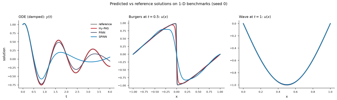
Figure 2.
Hy-PAS solution fields versus analytical reference on the two elliptic 2D benchmarks (seed 0). Left: reference; center: Hy-PAS prediction; right: pointwise absolute error. The Poisson error is a structureless speckle; the Helmholtz error concentrates in two horizontal bands, indicating an unresolved wavenumber.
Figure 2.
Hy-PAS solution fields versus analytical reference on the two elliptic 2D benchmarks (seed 0). Left: reference; center: Hy-PAS prediction; right: pointwise absolute error. The Poisson error is a structureless speckle; the Helmholtz error concentrates in two horizontal bands, indicating an unresolved wavenumber.
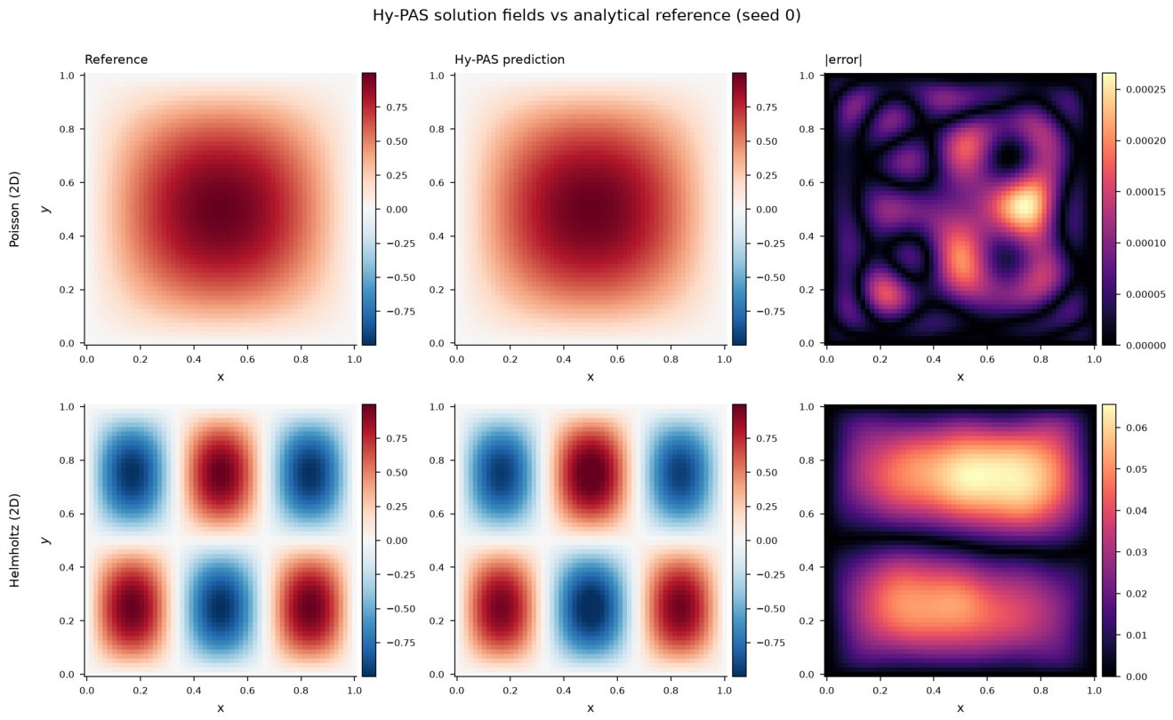
Figure 3.
Heat equation (2D, space–time). Left: peak amplitude decay versus time for reference and Hy-PAS; center and right: Hy-PAS field at and . Hy-PAS reproduces the diffusive decay of the solution.
Figure 3.
Heat equation (2D, space–time). Left: peak amplitude decay versus time for reference and Hy-PAS; center and right: Hy-PAS field at and . Hy-PAS reproduces the diffusive decay of the solution.
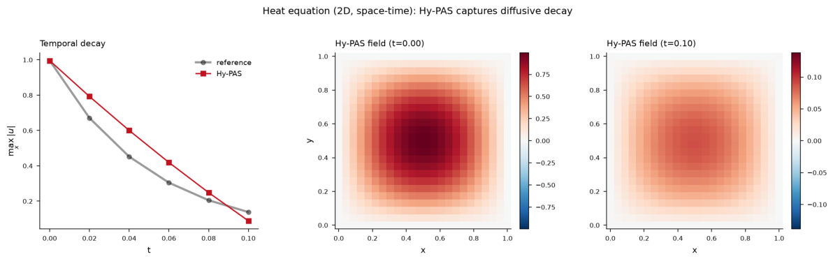
Figure 4.
Lid-driven cavity flow at : velocity magnitude and streamlines. Left: Ghia-validated finite-difference reference; right: Hy-PAS. Hy-PAS recovers the primary vortex structure but misses the secondary corner vortices, consistent with its relative error of on this hardest benchmark.
Figure 4.
Lid-driven cavity flow at : velocity magnitude and streamlines. Left: Ghia-validated finite-difference reference; right: Hy-PAS. Hy-PAS recovers the primary vortex structure but misses the secondary corner vortices, consistent with its relative error of on this hardest benchmark.
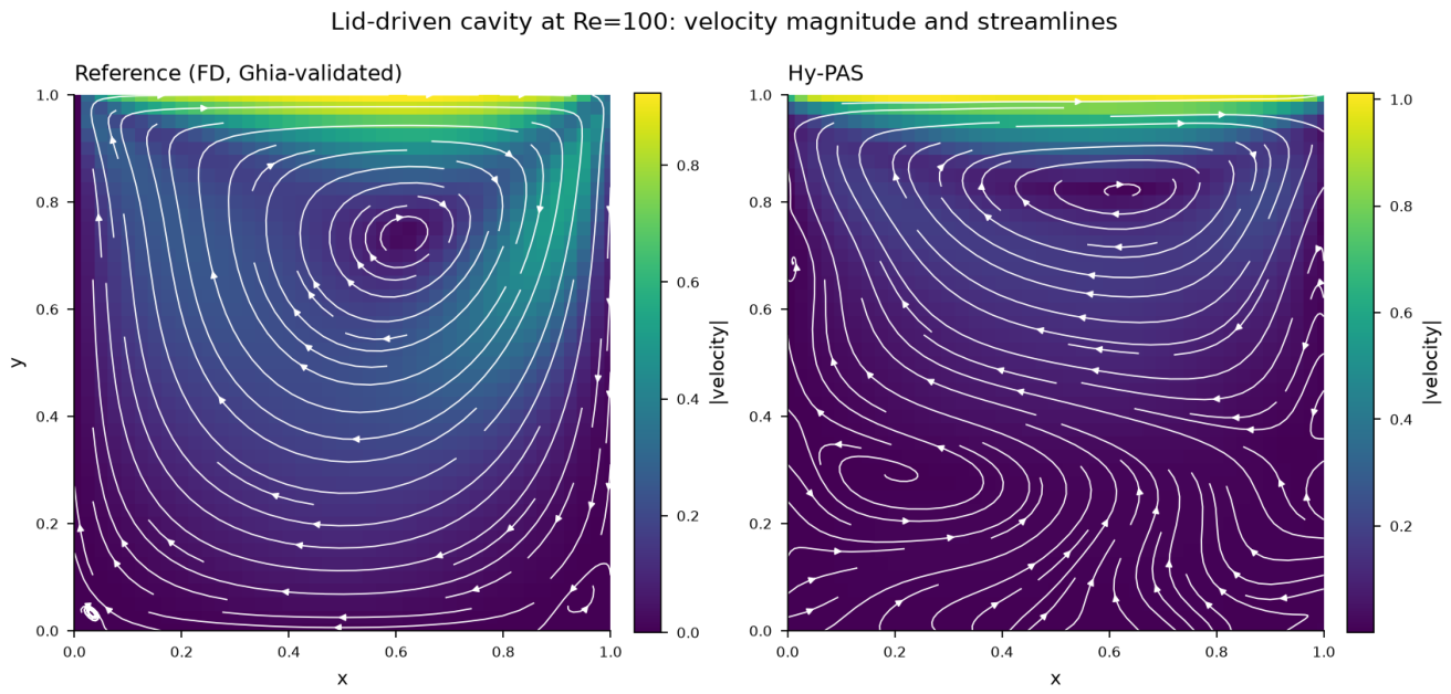
Figure 5.
Training convergence: relative error versus Adam iteration (mean over 3 seeds; shaded band = min–max envelope) on four representative benchmarks. Hy-PAS descends fastest and settles lowest on Poisson, wave, and the cavity; SPINN overtakes it on Helmholtz after iterations.
Figure 5.
Training convergence: relative error versus Adam iteration (mean over 3 seeds; shaded band = min–max envelope) on four representative benchmarks. Hy-PAS descends fastest and settles lowest on Poisson, wave, and the cavity; SPINN overtakes it on Helmholtz after iterations.
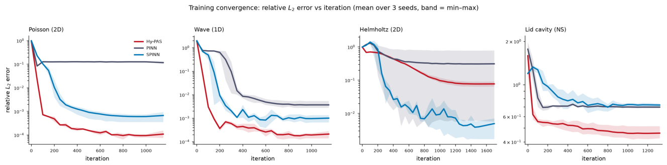
Figure 6.
Parameter-scaling study on Poisson (mean over 3 seeds). Left: relative error versus trainable parameter count—Hy-PAS reaches with a few hundred parameters and saturates, while the dense PINN plateaus near even at parameters. Right: CPU training time versus parameter count; on CPU Hy-PAS is not cheaper per parameter, as its scattered kernel evaluations do not map onto dense BLAS as efficiently as the PINN’s regular matrix multiplies.
Figure 6.
Parameter-scaling study on Poisson (mean over 3 seeds). Left: relative error versus trainable parameter count—Hy-PAS reaches with a few hundred parameters and saturates, while the dense PINN plateaus near even at parameters. Right: CPU training time versus parameter count; on CPU Hy-PAS is not cheaper per parameter, as its scattered kernel evaluations do not map onto dense BLAS as efficiently as the PINN’s regular matrix multiplies.
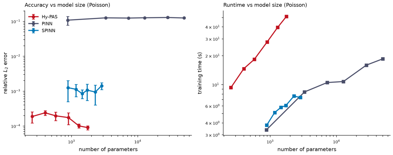
Figure 7.
Hy-PAS ablations (mean over 3 seeds, error bars = min–max). Left: kernel choice versus problem—the Wendland kernel matches the Gaussian on Poisson and wave but fails on the second-order damped ODE, where the Gaussian and multiquadric kernels are required. Right: sparsity–accuracy trade-off on Poisson—as the support radius grows the active connectivity rises from to while accuracy stays flat at .
Figure 7.
Hy-PAS ablations (mean over 3 seeds, error bars = min–max). Left: kernel choice versus problem—the Wendland kernel matches the Gaussian on Poisson and wave but fails on the second-order damped ODE, where the Gaussian and multiquadric kernels are required. Right: sparsity–accuracy trade-off on Poisson—as the support radius grows the active connectivity rises from to while accuracy stays flat at .
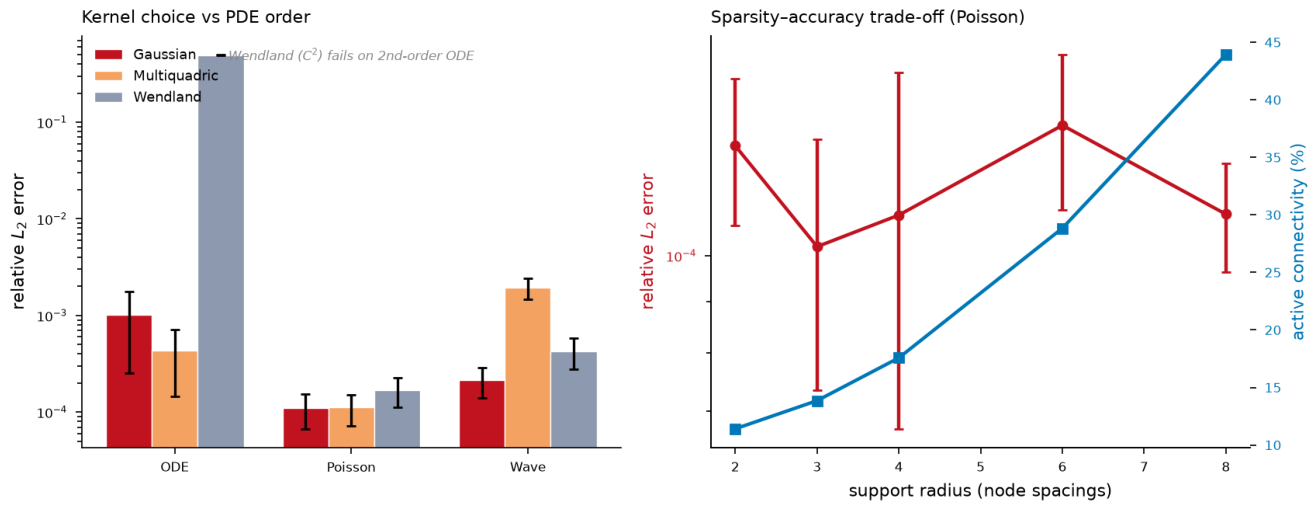
Figure 8.
Interpretability of the learned Hy-PAS parameters on the Helmholtz problem. Left: initial jittered-grid node layout. Center: node positions after training, with marker size ∝ learned amplitude and color encoding learned width . Right: shift in the width distribution from initialization to the trained model. Every parameter is a physical quantity, so inspecting the weights is inspecting the discretization.
Figure 8.
Interpretability of the learned Hy-PAS parameters on the Helmholtz problem. Left: initial jittered-grid node layout. Center: node positions after training, with marker size ∝ learned amplitude and color encoding learned width . Right: shift in the width distribution from initialization to the trained model. Every parameter is a physical quantity, so inspecting the weights is inspecting the discretization.
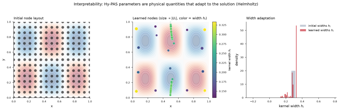

Table 1.
Qualitative positioning of Hy-PAS relative to representative neural PDE solvers along four axes. ✓ = yes, ✗ = no, (✓) = partial. Hy-PAS is simultaneously mesh-free, parameter-interpretable, structurally sparse, and basis-adaptive.
Table 1.
Qualitative positioning of Hy-PAS relative to representative neural PDE solvers along four axes. ✓ = yes, ✗ = no, (✓) = partial. Hy-PAS is simultaneously mesh-free, parameter-interpretable, structurally sparse, and basis-adaptive.
| Method | Mesh-free | Interpretable params | Structurally sparse | Adaptive basis |
|---|---|---|---|---|
| PINN [1] | ✓ | ✗ | ✗ | ✗ |
| Deep Ritz [2] | ✓ | ✗ | ✗ | ✗ |
| XPINN/cPINN [14,15] | ✓ | ✗ | (✓) | ✗ |
| FBPINN [16] | ✓ | ✗ | (✓) | ✗ |
| hp-VPINN [17] | ✓ | ✗ | (✓) | (✓) |
| DeepONet/FNO [18,19] | ✓ | ✗ | ✗ | ✗ |
| RBF collocation [20] | ✓ | ✓ | (✓) | ✗ |
| SPINN [5] | ✓ | (✓) | ✓ | ✗ |
| Hy-PAS (ours) | ✓ | ✓ | ✓ | ✓ |
Table 2.
Sparsity–accuracy trade-off for Hy-PAS on Poisson (225 nodes, mean over 3 seeds). The support radius (in units of node spacing) sets the fraction of active kernel–collocation connections. Accuracy is essentially flat from 11% to 44% connectivity, confirming that Hy-PAS operates in a genuinely sparse regime without loss of accuracy.
Table 2.
Sparsity–accuracy trade-off for Hy-PAS on Poisson (225 nodes, mean over 3 seeds). The support radius (in units of node spacing) sets the fraction of active kernel–collocation connections. Accuracy is essentially flat from 11% to 44% connectivity, confirming that Hy-PAS operates in a genuinely sparse regime without loss of accuracy.
| Support radius | Active connectivity | rel. error |
|---|---|---|
| 2 | 11.4% | |
| 3 | 13.9% | |
| 4 | 17.6% | |
| 6 | 28.8% | |
| 8 | 43.9% |
Table 3.
Kernel ablation for Hy-PAS: relative error (mean over 3 seeds) for three radial kernels of differing smoothness. The compactly-supported Wendland kernel is accurate on the first-order-dominated Poisson and Wave problems but fails on the second-order damped ODE, where the Gaussian and inverse-multiquadric kernels are required. Kernel smoothness must match the differential order of the operator.
Table 3.
Kernel ablation for Hy-PAS: relative error (mean over 3 seeds) for three radial kernels of differing smoothness. The compactly-supported Wendland kernel is accurate on the first-order-dominated Poisson and Wave problems but fails on the second-order damped ODE, where the Gaussian and inverse-multiquadric kernels are required. Kernel smoothness must match the differential order of the operator.
| Kernel | ODE | Poisson | Wave |
|---|---|---|---|
| Gaussian | |||
| Multiquadric | |||
| Wendland | 0.495 |
Table 4.
Trainable parameter count and wall-clock training time (s, CPU, mean over 3 seeds) for each method. Hy-PAS attains its accuracy with roughly an order of magnitude fewer parameters than the dense PINN.
Table 4.
Trainable parameter count and wall-clock training time (s, CPU, mean over 3 seeds) for each method. Hy-PAS attains its accuracy with roughly an order of magnitude fewer parameters than the dense PINN.
| Hy-PAS | PINN | SPINN | ||||
|---|---|---|---|---|---|---|
| Benchmark | params | time | params | time | params | time |
| ODE (damped) | 450 | 11 | 12673 | 12 | 881 | 2 |
| Poisson 2D | 900 | 38 | 12737 | 15 | 1729 | 8 |
| Helmholtz 2D | 900 | 79 | 12737 | 28 | 1729 | 20 |
| Heat 2D | 1080 | 101 | 12801 | 31 | 2577 | 32 |
| Burgers 1D | 800 | 54 | 12737 | 20 | 1729 | 13 |
| Wave 1D | 800 | 37 | 12737 | 16 | 1729 | 9 |
| Lid cavity (NS) | 1350 | 159 | 12867 | 58 | 1795 | 37 |
Table 5.
Relative error on seven benchmarks (mean over 3 random seeds). Best per row in bold. Hy-PAS, PINN, and SPINN are each tuned with a fixed protocol (Adam + L-BFGS polish); learning rates respectively.
Table 5.
Relative error on seven benchmarks (mean over 3 random seeds). Best per row in bold. Hy-PAS, PINN, and SPINN are each tuned with a fixed protocol (Adam + L-BFGS polish); learning rates respectively.
| Benchmark | Hy-PAS | PINN | SPINN |
|---|---|---|---|
| ODE (damped) | 0.219 | 0.601 | |
| Poisson 2D | 0.118 | ||
| Helmholtz 2D | 0.312 | ||
| Heat 2D | 0.178 | 0.269 | |
| Burgers 1D | 0.122 | 0.323 | |
| Wave 1D | |||
| Lid cavity (NS) | 0.461 | 0.699 | 0.722 |
Table 6.
Parameter-scaling study on the Poisson benchmark: relative error as a function of trainable parameter count (mean over 3 seeds). Hy-PAS reaches with a few hundred parameters and saturates; the dense PINN plateaus near even at parameters.
Table 6.
Parameter-scaling study on the Poisson benchmark: relative error as a function of trainable parameter count (mean over 3 seeds). Hy-PAS reaches with a few hundred parameters and saturates; the dense PINN plateaus near even at parameters.
| Hy-PAS | PINN | SPINN | |||
|---|---|---|---|---|---|
| params | rel. | params | rel. | params | rel. |
| 256 | 881 | 0.109 | 889 | ||
| 400 | 3297 | 0.127 | 1169 | ||
| 576 | 7249 | 0.125 | 1449 | ||
| 900 | 12737 | 0.127 | 1729 | ||
| 1296 | 28321 | 0.130 | 2289 | ||
| 1764 | 50049 | 0.126 | 2849 | ||
Disclaimer/Publisher’s Note: The statements, opinions and data contained in all publications are solely those of the individual author(s) and contributor(s) and not of MDPI and/or the editor(s). MDPI and/or the editor(s) disclaim responsibility for any injury to people or property resulting from any ideas, methods, instructions or products referred to in the content. |
© 2026 by the authors. Licensee MDPI, Basel, Switzerland. This article is an open access article distributed under the terms and conditions of the Creative Commons Attribution (CC BY) license (http://creativecommons.org/licenses/by/4.0/).
Copyright: This open access article is published under a Creative Commons CC BY 4.0 license, which permit the free download, distribution, and reuse, provided that the author and preprint are cited in any reuse.