

Submitted:
14 August 2026
Posted:
17 August 2026
You are already at the latest version
Abstract
Extreme wind speed poses significant risks to the economy in areas such as infrastructure and agriculture in South Africa, particularly in semiarid regions such as the Northern Cape. In minimizing such risks, accurate modelling of extreme wind speed is essential for disaster preparedness and climate adaptation. In this pursuit, Hybrid Generalised Additive Extreme Value (GAEV) models have been used in climate studies, where the extreme value parameters are allowed to evolve smoothly through spline functions of the covariates to improve forecasts. However, such applications remain limited and scattered across literature. Furthermore, comparative evaluations of the performance of the hybrid models estimated via frequentist and Bayesian estimation approaches with applications to extreme wind speed remain scarce, particularly within semi-arid regions of South Africa. This creates a gap in both literature which the study seeks to bridge. To achieve this, we estimate the hybrid GAEV models via frequentist (maximum likelihood) and Bayesian methods using extreme wind speed data from Kimberley and Upington in the Northern Cape Province of South Africa. We then compare the performance of the two estimation frameworks using metrics such as Root Mean Squared Error (RMSE), Mean Absolute Error (MAE), and Mean Absolute Percentage Error (MAPE). The results shows that the Bayesian GAEV consistently outperformed the frequentist approach, producing lower error values in both in-sample and out-of-sample forecasts. This demonstrates the Bayesian framework’s superior ability to capture non-linear covariate effects and tail behaviour in extreme wind distributions. The findings highlight the importance of Bayesian GAEV models for reliable forecasting of extreme wind speeds in vulnerable regions. Policymakers and disaster management agencies should adopt Bayesian based approaches to improve risk assessment and preparedness strategies. Future research should extend the analysis to additional provinces, incorporate longer datasets, and explore broader climatic drivers to enhance generalisability and strengthen climate resilience planning.
Keywords:
Bayesian
; Extreme Value Theory
; frequentist
; Generalised Additive Extreme Value
1. Introduction
Climate change is a major concern facing the world today, with extreme events increasingly having impacts on property, infrastructure, economy, and agriculture. These events are broadly defined as the time and location where weather, climate, or environmental conditions exceed the usual range of what has occurred in the past [1]. Within South Africa, the Northern Cape province stands out as a semi-desert province where strong winds frequently affect the communities, threaten infrastructure and agricultural productivity. Considering these significant impacts of extreme events, it is therefore imperative to study their patterns to help better preparedness.
Extreme event studies have increasingly become important due to increased changes in the world climate. Different extreme value and additive frameworks which have been mostly useful in modelling and forecasting extreme weather events include the Generalised Extreme Value (GEV) [2], Generalised Additive Models (GAMs) and Bayesian Generalised Extreme Value (GEV) models, among others [3]. Recent works has employed a hybridisation of the framework called Generalised Additive Extreme Value (GAEV) to model extreme events by allowing extreme value parameters to depend on covariates through spline functions [4]. However, such applications remain limited and scattered across hydrology and environmental science. Furthermore, while Bayesian methods have been increasingly recognised for their ability to incorporate prior information and quantify uncertainty [5,6,7], comparative studies among Bayesian and frequentist approaches in general and extreme wind speed modelling context remain scarce, particularly in semi-arid regions. In South Africa, and specifically in semi-arid regions such as the Northern Cape, extreme wind events pose significant risks to infrastructure, agriculture, and livelihoods. Yet, empirical studies applying advanced statistical frameworks to localised wind extremes are limited. From the limited studies, very few have used hybrid GAEV which offer better predictive performance by adequately capturing the underling properties of the extreme events, but the focus has been limited to temperature and rainfall extremes. In addition, comparative studies of the performance of the hybrid GAEV models estimated via maximum likelihood and Bayesian estimation approaches with applications to extreme wind speed remain scarce, particularly within semi-arid regions of South Africa. Therefore, there is a need to fill this gap, owing to the need for accurate modelling and forecasting of wind speed in semi-arid regions.
This study addresses these gaps by extending and applying the hybrid GAEV framework to a new and practically important problem; extreme wind speed modelling in semi-arid South Africa and then provide a comparison between Bayesian and frequentist estimation within this framework. The extension of the GAEV framework allows the parameters of the GEV distribution (location, scale, and shape) to vary smoothly with covariates such as seasonality, temperature, humidity, and cloud cover via spline functions. The method is then used to fit wind speed data from Kimberley and Upington stations, to the frequentist and Bayesian versions of the hybrid model. Subsequently, the performance of the two approaches is compared to identify the most accurate method.
The originality of this study lies in its formalization or extension of the GAEV framework to explicitly use splines to allow the location, scale, and shape parameters to vary smoothly with covariates such as seasonality, temperature, humidity, and cloud cover to capture non-linear influences on extreme wind behaviour more effectively. A further novel contribution is the explicit comparison between frequentist and Bayesian estimation of GAEV models. By employing the maximum likelihood estimation alongside Bayesian inference via Markov Chain Monte Carlo (MCMC). We then compare the performances of the frequentist and Bayesian approaches. This comparative evaluation is relatively underexplored in African climate modelling literature and demonstrates the practical advantages of Bayesian approaches for forecasting extremes.
Finally, the application of this framework to extreme wind speed events in Kimberley and Upington, represents a significant regional innovation. The Northern Cape is a semi-arid, climate sensitive region where infrastructure, agriculture, and livelihoods are highly vulnerable to wind extremes. By employing advanced statistical modelling within this context, the study contributes to region specific insights that can inform disaster preparedness, infrastructure planning, and climate adaptation strategies. For the rest of the paper, the materials and methods are presented in Section 2, the results and discussions in Section 3 while the conclusion is presented in Section 4.
2. Materials and Methods
2.1. Study Source and Area
The data used in this paper consist of the maximum daily temperature, maximum relative humidity, maximum cloud cover, and maximum wind speed from 1 January 2019 to 31 December 2024. The data was specifically sourced from the Open-Meteo API which is available at https://open-meteo.com/en/docs/historical-weather-api. The specific areas of interest are Kimberley and Upington, located in the Northern Cape Province of South Africa. These areas have predominantly semi-arid climates, see Figure 1, which makes them appropriate for this study.
The dataset consisted of hourly observations, which were aggregated to daily maximum wind speed to have a block maxima data for the extreme value analysis. The aggregation of hourly observations to daily maximum resulted in a loss of information regarding the "within day" variability and the timing and duration of extreme wind events.
2.2. Test for Stationary
As highlighted by [8], assessing stationarity and the existence of unit roots remains a fundamental step in time series analysis because these properties directly affect model specification, estimation, and forecasting accuracy. Since many statistical time series techniques are developed under the assumption that the underlying process is stationary, it is important to verify this assumption before proceeding with further analyses in the present study. To evaluate stationarity, three widely used procedures are employed, namely the Augmented Dickey–Fuller (ADF), Phillips–Perron (PP), and Kwiatkowski–Phillips–Schmidt–Shin (KPSS) tests. The Augmented Dickey–Fuller (ADF) test is a commonly applied method for examining whether a time series contains a unit root and is therefore non-stationary [9]. By accounting for higher-order serial correlation through lagged difference terms, the ADF test provides a robust framework for determining the stationarity properties of a series. The hypotheses considered in the test are given as follows:
- : the time series contains a unit root, non-stationary;
- : the time series does not contain a unit root, stationary.
The ADF test uses a regression model:
where is a constant, is the coefficient on time trend, and represents the white noise process. The null hypothesis is , and the alternative hypothesis is .
The PP test is closely related to the ADF test. It serves as an alternative to the ADF test and applies non-parametric corrections to account for serial correlation and heteroskedasticity in the error terms [10].The hypothesis for the PP test is formulated as indicated below:
- time series has a unit root, non-stationary;
- time series does not have a unit root, stationary.
The test involves the estimation of the regression equation:
where represents the time series, is the intercept, is a deterministic time trend, is the autogressive coefficient, and is a white noise error term.
The KPSS test models a time series as:
where is a deterministic trend, is a stationary error term, and is a random walk which is then expressed as
where .
The KPSS test assumes the time series data is stationary under the null hypothesis and non-stationary under the alternative hypothesis, i.e.,
- time series is stationarity;
- time series not stationarity.
If , then is constant and time series is stationary. If , then time series is non-stationary and follows a stochastic trend.
The KPSS test statistic is calculated as:
A high KPSS statistic value suggests the presence of a unit root and a low KPSS value means the null hypothesis of stationarity canoot be rejected.
2.3. Normality Tests
The normality tests are usually used for checking normality, that is, if the data are normally distributed or not. This paper used the Shapiro-Wilk (SW) and Jarque-Bera (JB).
SW tests the null hypothesis that the data are normally distributed against the alternative that it is not. According to [11], the null hypothesis is rejected when then value of W statistic is small and the p-value is less that the specified level of significance which indicates a significant deviation from normality.
The SW test is given as:
where is the ith order statistic and is the sample mean.
The coefficient are given by:
where
are the expected values of the order statistic of independent and identically distributed random variables from the standard normal distribution and V is the covariance matrix of the order statistic.
The JB is also a normality test that is widely used due to its simplicity and satisfactory performance [12]. The test is defined as:
where n is the number of observations , S is the sample skewness, and K is the sample kurtosis:
The hypothesis test:
- the series follows a normal distribution;
- the series does not follow a normal distribution.
2.4. Goodness-of-Fit
The Goddness-of-Fit (GoF) tests statistics are usually used for checking the validity of an assume probability distribution model, i.e to evaluate how well the GEVD explains extreme event. This paper used the Kolmogorov-Smirnov (KS) test the Anderson-Darling (AD). According to [13] the KS test is a non-parametric test applied to test whether the sample under consideration is from a hypothesised distribution or to compare whether two samples come from identical distribution. The hypotheses are formulated as:
- for all x from , i.e., the series follows a specified distribution;
- the series does not follow the specified distribution.
The test statistic is also defined as:
The null hypothesis for this test is rejected at 5% significance level if calculated is greater than the tabulated value
Meanwhile, AD test is used to assess whether data comes from a specified distribution with the hypotheses formulated as
- the series follows a specified distribution;
- the series does not follow a specified distribution.
The test statistic is defined as:
where the data x is the ordered sample of size n, and is the theoretical CDF to which the sample is compared. The A-D test assign more weight to the tail of the distribution than the K-S test.
2.5. Generalised Additive Models
Generalised Additive Models (GAMs) are an extension of the generalised linear models (GLM)
where Y is the response variable, is the expected value of the response, is the link function (connects the mean of Y to the linear predictor), are the model coefficients and are the independent variables. The GAMs allow non-linear relationships between predictors and the response through the use of smooth functions [14]. GAMs extend Generalised Linear Models (GLMs) by incorporating smooth functions of the predictors.
Let Y be a response random variable and be a set of k independent variables. GAMs consists of a random component, an additive component, and a link function relating to the two component,
where is a link function, is the expected value of the response variable, is the constant, are the independent variables and are smooth functions of the predictor variable. The smooth functions are usually fit using non-parametric curve estimating methods such as the local-regression, splines, or smooth splines.
GAMs focuses on exploring data non-parametrically and are more suitable for exploring the data set and visualising the relationship between the dependent variable and the independent variables [15].
2.6. Extreme Value Theory
Extreme Value Theory (EVT) is known as the study of extremal properties of random processes and its objective is to quantify the stochastic behaviour of a process as usually high or low levels. According to [16], the intention to use the EVT is to predict the occurrence of extreme or rare events using historical data. Block maxima and the peaks-over-threshold (POT) are the two fundamental approaches in EVT.
2.6.1. Generalised Extreme Value Distribution
The Generalised Extreme Value Distribution (GEVD) arises from the theory of extreme values and provides a unified framework for modelling rare and extreme events [17]. It is typically applied using the block maxima approach, where the largest observation within each predefined time block is extracted for analysis. Under the extreme value theorem, the distribution of suitably standardised block maxima converges to the GEVD as the sample size becomes large. Consequently, the GEVD is well suited for analysing maxima obtained from independent and identically distributed (.) observations collected over fixed intervals. As noted by [18], the GEVD is frequently adopted as an approximate probability model for the largest values observed within sufficiently long sequences of random variables. A notable feature of the GEVD is that it encompasses three classical extreme value distributions, namely the Gumbel, Fréchet, and Weibull distributions, commonly referred to as Type I, Type II, and Type III extreme value distributions, respectively. By incorporating these distributions into a single family, the GEVD is capable of representing a wide variety of tail behaviours and distributional shapes through a common modelling framework.
where , and are the location, scale and shape parameters, respectively. For , and . For Equation (15) is the Gumbel class of distribution which is given by
For and , the distribution in Equation (15) corresponds to the Fréchet and negative Weibull distributions, respectively. The location parameter specifies where the distribution is centred, the scale parameter reflects the degree of variability in the data, and the shape parameter influences the nature of the distribution’s tails.
The GEVD’s extreme quantiles are estimated as follows:
Here, represents the return period and is known as the return level associated with the return period . This is the level which is expected to be exceeded on average once every years. The GEVD allows us to model the extreme values of block maxima.
2.6.2. Generalised Pareto Distribution
Within the Peaks-Over-Threshold (POT) framework, the Generalized Pareto Distribution (GPD) is commonly employed to describe observations that exceed a suitably chosen threshold. In extreme value analysis, it is particularly useful for characterizing the tail behaviour of an underlying distribution. The GPD has three parameters, the threshold parameter , the shape parameter and the scale parameter . The GPD is considered the most efficient distribution compared to the GEVD, the equation is given by:
where and . Equation (18) becomes an exponential distribution when and uniform when . When , the distribution has a finite end point and is referred to as short-tailed. When , the distribution is referred to as heavy-tailed.
2.6.3. Parameter Estimation
By employing maximum likelihood and Bayesian method to estimate the parameters , we will gain a valuable insight into the behaviour of the extreme events, under study.
The Maximum Likelihood Estimation Method
Parameter estimation under the maximum likelihood framework is achieved by identifying the set of parameter values that maximizes the likelihood function associated with the assumed probability distribution [19]. It is a widely used method for estimating parameters in statistical models [20] and it is an effective method when dealing with large samples. However, it is know to performs badly when the sample size is small.
Consider a sample of independent and identically distributed observations drawn from a GEVD. For , the log-likelihood funct is given by:
where and . When , the log-likelihood function becomes:
Let be a random sample of n with extreme value above a threshold u, the log-likelihood function of the GPD be expressed as
provided for . The likelihood function may be rewritten as
Bayesian Method
Bayesian estimation of GEVD parameters involves updating prior beliefs using the likelihood derived from observed data. This process yields a posterior distribution that reflects both prior assumptions and sample information, resulting in a more comprehensive understanding of the parameters [19]. The model parameters are not usually random, but they are, however, treated as random by assigning probability distributions to describe the uncertainty of their values. The Bayesian method uses a computational algorithm called Markov Chain Monte Carlo (MCMC) to estimate the posterior distributions of model parameters. The parameter estimation is made through the posterior distribution which is computed using Bayes’ Theorem:
where is the posterior distribution of , is the likelihood function, is the prior distribution which represents prior knowledge about the parameters, and is the marginal likelihood. The Bayesian GAMs estimation:
where y is the independent variable being observed, is the posterior distribution of the intercept and smooth functions, is the likelihood which describes how the data relate to the model, is the prior on the intercept, is the prior on the smooth function, and is the product over all smooth function priors, assuming they are independent. Suppose are iid and their distribution fall within the GEV or GPD family. The parameters are treated as random variables.
where is the posterior distribution of the GEVD/GPD parameter, is the likelihood, and are the prior distributions.
2.7. Generalised Additive Extreme Value
Rather than using the GAMs and EVT separately, this paper integrates them through the Generalised Additive Extreme Value (GAEV) model allowing the GEV parameters to vary smoothly with covariates. The GAEV model is a hybrid model that combines the flexibility of GAMs with the principles from EVT [4]. The GAMs framework allows us to model the non-linear effects of covariates on the GEVD parameters.
Let be a random variable that depends on the covariate x, such that
where parameters are modelled as smooth functions of covariates through GAMs.
The location model:
the log scale model:
and the shape model:
where and are intercepts, and and and are non-linear functions that include seasonality (day of year), maximum temperature, maximum relative humidity, and maximum cloud cover.
The GAEV model is usually applied to model the distribution of block maxima, allowing the estimation of return levels.
2.8. Model Selection
Model selection involves choosing the best model from a list of candidates based on data analysis [21]. Akaike Information Criterion (AIC), Bayesian Information Criterion (BIC), and Leave-One-Out Cross Validation (LOO-CV) are selection models that are used to compare how well statistical models fit data.
AIC aims to find the model that best explains the data with the fewest number of parameters, hence balancing goodness of fit and model complexity. Given the number of parameters in the model as k and L as the estimated likelihood, the AIC is formulated as. A model with the lowest AIC value is preferred.
Using similar definitions for k and L, the BIC is also fromulated as,
where n is the number of data points. BIC selects a model that maximises the posterior model probability. Unlike the AIC and the BIC which are used to compare the performance of any two models, the LOO-CV is used to assess the fitness of different estimated Bayesian models [7].
2.9. Model Diagnostics
Model diagnostics includes using various tools and techniques to check model validity and assumptions, they assess how well a chosen model fits the data [22] and whether it satisfies the necessary assumptions of the modeling framework. Another way of assessing the goodness-of-fit is by utilizing the diagnostic plots; Probability-Probability (P-P), Quantile-Quantile (Q-Q), Residuals vs. Seasonality, and Density Histogram.
The P-P plot compares the empirical probabilities to the theoretical probabilities. For a good fitted model, the empirical probabilities will overlap with the theoretical probabilities to form a straight diagonal line. plots [23]. Checks the overall distribution fit.
The Q-Q plot compares the empirical quantiles and the theoretical quantiles from the fitted model, deviations from the diagonal line shows a mismatch in tail estimation [23]. It checks the tail behaviour and overall fit of the GEV.
The residual vs seasonality plot examines whether seasonal structure has been adequately captured by the smooth terms.
The density histogram compares the empirical and fitted density of the maxima.
2.10. Metrics for Evaluating Forecasts
Forecast evaluation assesses how well the fitted model predicts unseen or future data. It helps with comparing and assessing model performance. Evaluating the effectiveness of our models, the following metrics are to be applied; Root Mean Squared Error (RMSE), Mean Absolute Error (MAE), and Mean Absolute Percentage Error (MAPE). The values of RMSE, MAE, and MAPE can measure how how good the prediction results produced by a model are [24]. Given n as the length of the sample, as the actual value and as the predicted value, the metrics are calculated as follows:
3. Results and Discussion
3.1. Exploratory Data Analysis
3.1.1. Summary Statistics
Table 1 shows the descriptive statistics of both Kimberley and Upington stations. With Kimberly showing the maximum wind speed of and average of . And Upington showing the maximum wind speed of and an average of . The distribution of Kimberley a positive skewness since the value is positive and a platykurtic given the kurtosis value is more than 3 which implies more extreme wind speed events. While Upington also shows a positive distribution and leptokurtic with a kurtosis value of less than 3 which means fewer extreme wind speed events.
3.1.2. Stationarity Tests
Table 2 presents the results of the stationary test for the daily maximum wind speed for Kimberly, and Upington.
Evidence from the table suggests that the time series data are stationary for all the stations. This is because the p-values for the ADF, PP and KPSS tests are all less than the level of significance. Overall, the ADF and PP results show strong evidence that the daily maximum wind speed data at all stations are stationary.
3.1.3. Test for Normality Results
Table 3 presents the normality test for the daily maximum wind speed. S-W and J-B test results show that the null hypothesis of normality is rejected at level of significance for the daily maximum wind speed across all stations. These results are consistent with the kurtosis values from Table 1. In conclusion, evidence from the table indicate that the daily maximum wind speed for both stations do not follow a normal distribution.
3.2. Model Fitting Results
3.2.1. Estimated Frequentist Parameters
The table below, Table 4, presents the parametric intercept estimates and their corresponding standard error (in parantheses) for the GEV parameters; the location, scale, and shape.
From the table, there is clear evidence that Upington has the highest location intercept, under the Location model, implying higher extremes, with 19.50, than Kimberley. The shape intercepts are negative for both stations, suggesting a Weibull distribution, upper bounded tails and finite maximum wind speed.
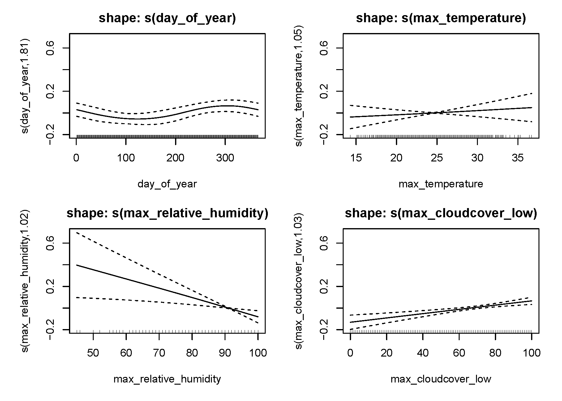
The tables below, Table 5 and Table 6, present smooth terms for Kimberley and Upington. The estimated degrees of freedom (edf) determines the flexibility of the curve; an edf value closer to 1 means the term behaves like a straight line (there is a linear effect) and an edf greater than 1 means the term captures non-linear patterns. Furthermore, the importance of these smooths are checked through the p-values, [4].
The result shows that day of year (seasonality trend) and temperature have highly significant smooth effects in the Location model. The day of year smooth term shows high significance across all models in both stations which indicates strong evidence of seasonal effects on the daily maximum wind speed.
In Kimberley, Table 5, all the smooth terms are significant across all models except for maximum cloudcover under the Scale model. The smooth terms showing non-linear relationships except the maximum cloudcover under the Shape model with edf = 1.01.
Table 6, the Location and Scale models have significant smooth terms. The smooth terms show approximately linear effects on the Shape model, however, maximum temperature seems insignificant with p-value more than 0.05.
Overall, the Location model seems to produce more highly significant terms over the Scale and Shape models. (see Appendix A).
3.2.2. Goodness-of-Fit Tests for Extreme GAMs
Table 7 presents the Kolmogorov-Smirnov (K-S) and Anderson-Darling (A-D) goodness-of-fit test results for Kimberley and Upington stations using the mle parameters.
From Table 7, the p-values for both tests are higher than 5% thus the tests are statistically insignificant for the location model across both stations. This implies that the daily maximum wind speed follows the specified GAEVD model, that is, the Location model fits well. As for the Scale model Upington show highly significant p-value, leading to the rejection of the null hypothesis and the conclusion that the station does not follow the specified GAEVD model while Kimberley does follow the specified GAEVD model. The p-values for Kimberly shows insignificance under the Shape model which implies that the daily maximum wind speed follows the specified GAEVD model while Upington does not follow the GAEVD model since the p-values are all less than 5%. Similarly, the table provides clear evidence that the maximum daily wind speed follows the specified GAEVD model in Kimberly stations.
Figure 2 and Figure 3 below display four standard diagnostic plots for the best fitted model, Location model. From each figure, the top-left is the Probability-Probability (P-P) plot, top-right is the Quantile-Quantile (Q-Q) plot, bottom-left is the Residual vs Seasonality plot, and bottom-right is the Density Histogram of Residuals plot. The figures show that the P-P and Q-Q plots are almost linear illustrating a good fit of the GEV to the daily maximum wind speed. The density histogram shows a positive skewness across both stations.
3.2.3. Model Selection
Table 8 presents model selection. The best model is seelected using Akaike Information Criterion (AIC) and Bayesian Information Criterion (BIC). The lowest values of the AIC and BIC represent the best model.
The Location model produced lower values across both stations, this implies that Location model is the best fitted model, with Kimberley having the lowest AIC and BIC values. Since the Location model outperforms the Scale and Shape models, this indicates that changes in the central tendency are the best explanation for extremes, rather than variations in dispersion or tail heaviness.
3.2.4. Metrics Evaluation
Table 9 presents the RMSE, MAE, and MAPE evaluation metrics used to assess the forecasting performance of the Location, Scale, and Shape models, for both in-sample and out-of-sample. The model with the smallest RMSE, MAE, and MAPE is considered the best model. In the in-sample metrics evaluations performance, the Location model demonstrated better performance than the Scale and Shape models across all metrics. The results show that the Location model gives the most precise representation of extremes (better predictive accuracy), with lower RMSE, MAE, and MAPE values, while Scale and Shape models show weaker performances across both stations.
Kimberley produced the lowest metrics value under the Scale model, in the out-of-sample performance, indicating that the Scale model gives better predictive accuracy. Similarly, the Scale model performs better than the Location and Shape for Upington. Overall, Scale model produces lower metrics values across all stations, in the out-of-sample performance.
3.2.5. Return Level
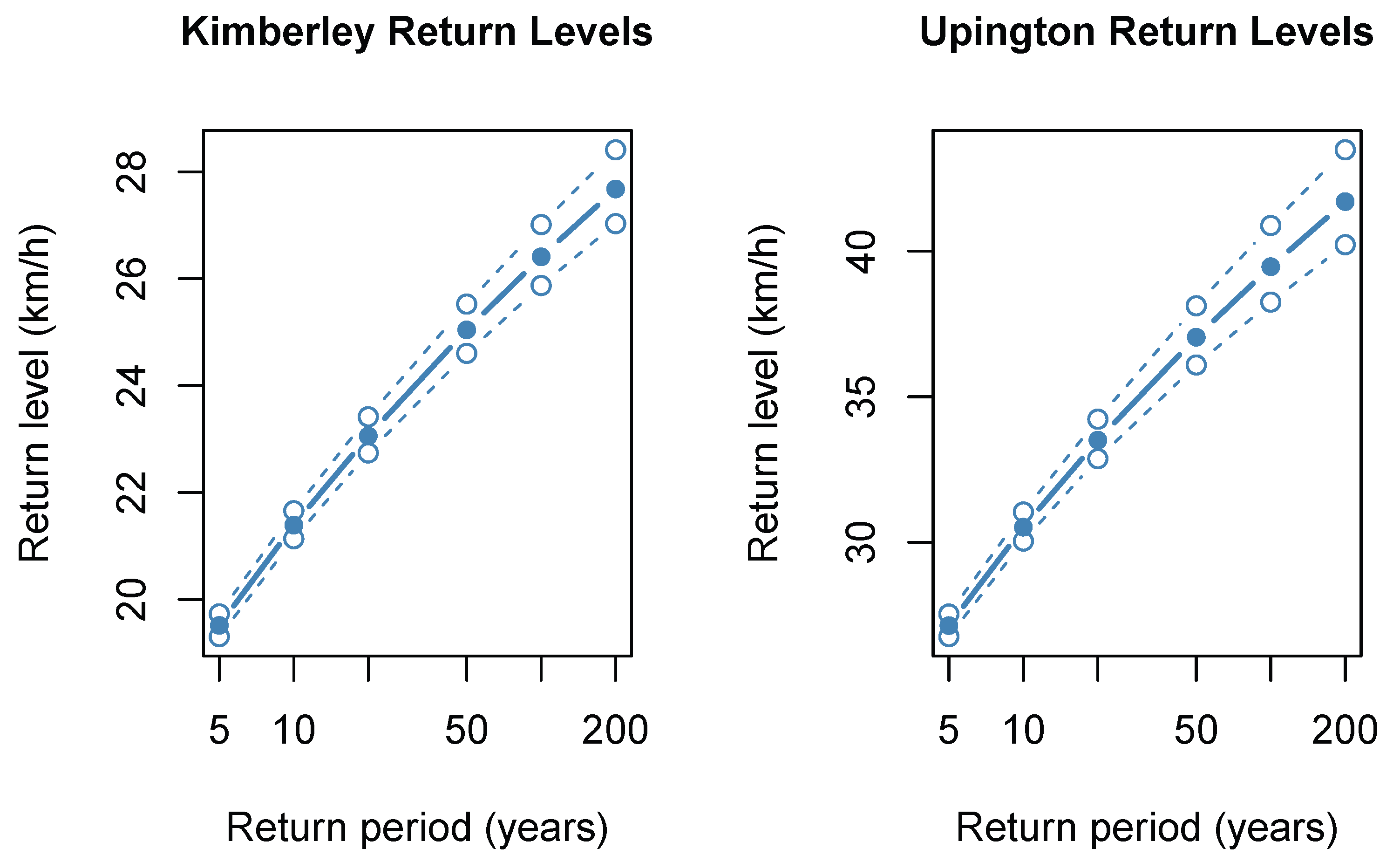
The return level estimates for daily maximum wind speed at different return periods are given in Table 10, and the accompanying 95% confidence intervals are shown in parentheses.
The results in the table shows the return levels increase as the periods increase. Kimberley has the lowest 5 year return level of 19.51 km/h with a narrower confidence interval ranging from 19.30 km/h to 1973 km/h and Upington has 27.14 km/h return level with a bit wider confidence interval ranging from 26.76 km/h to 27.54 km/h. This suggests that a maximum wind speed of 19.51 km/h is expected to increase atleast once in 5 years. 41.71 km/h maximum wind speeds are expected to increase atleast once in 200 years in Upington and 27.68 km/h in Kimberley. From the table, it is clear that Upinton will experience more increase in the wind speed along the years as compared to Kimberly.
The figure, Figure 4, below depicts the return levels plots for the stations Kimberley and Upington.
3.3. Diagnostics of Estimated Bayesian Extreme GAMs
The performance and convergence of the Bayesian GAEV models were assessed using posterior probability plots, the Gelman–Rubin statistic (Rhat), Bulk ESS, Tail ESS, and LOO criteria [7]. Table 11 and Table 12 present the corresponding diagnostic results for the location, scale, and shape models. Since all estimated parameters, namely day of year, temperature, relative humidity, and cloud cover, yielded Rhat values of 1, there is strong evidence that the MCMC chains converged successfully and produced reliable posterior estimates.
3.3.1. Goodness-of-Fit Test for Extreme GAMs
Using the posterior parameter estimates derived from the Bayesian analysis, goodness-of-fit diagnostics were performed to evaluate the appropriateness of the fitted GAEVD model. In particular, the K–S and A–D tests were applied to examine whether the distribution of daily maximum wind speed observations is consistent with the assumed GAEVD model.
The goodness-of-fit statistics reported in Table 13 provide evidence regarding the suitability of the Bayesian GAEVD models for the two study locations. For the model governing the location parameter, both the K–S and A–D procedures produced probability values above the conventional 0.05 threshold for Kimberley and Upington. As a result, the assumption that the observed daily maximum wind speed data originate from the fitted GAEVD cannot be rejected, indicating satisfactory model performance at both stations. Different conclusions emerge for the scale component. While the Kimberley results remain compatible with the fitted distribution, the corresponding outcomes for Upington suggest a lack of agreement between the observed data and the assumed model. This is reflected by statistically significant test results, with reported probability values of approximately 0.005. Consequently, the hypothesis that the scale model adequately represents the Upington data is not supported. With respect to the shape component, the diagnostic tests again reveal contrasting behaviour between the two sites. The Kimberley station exhibits probability values exceeding the 5% significance level, providing no indication of a departure from the fitted GAEVD. In contrast, the corresponding values for Upington fall below the specified significance threshold, suggesting that the fitted shape model does not adequately capture the characteristics of the daily maximum wind speed observations at that location.
3.3.2. Model Performance
The table below, Table 14, presents the LOO-CV tests results. The prediction accuracy is measured by the expected logarithmic predictive density (elpd_loo) and leave-one-out information criterion (looic) compares the model(s). The highest elpd_loo and lowest looic values indicate better model (superior model) performance over other models, and the pareto estimates evaluates the reliability of the model where the values less than 0.7 indicate the results are stable and reliable.
From the table, there is clear evidence that the Location model outperforms the Scale and Shape model across both stations. Kimberley has a higher elpd_loo of -5605. and lower looic of 9234.9 value for the Location model, making the Location model superior over Scale and Shape models. Overall, the Location model performs better than the Scale and Shape models due to higher elpd_loo and lower looic values. Additionally, since the pareto estimates for all the models and across the stations are less than 0.7, that is an indication that the models are reliable and stable.
3.3.3. Metrics Evaluation
Table 15 presents the Root Mean Square Error (RMSE), Mean Absolute Error (MAE), and Mean Absolute Percentage Error (MAPE) evaluation metrics used to assess the forecasting performance of the Location, Scale, and Shape models, for both in-sample and out-of-sample. The model with the smallest RMSE, MAE, and MAPE is considered the best model.
The in-sample performance shows that the location model performs better than the Scale and Shape models across all metrics. These results show that the Location model gives the most precise representation of extremes (better predictive accuracy), with lower RMSE, MAE, and MAPE values, while Scale and Shape models show weaker performances across both stations.
Similar to the in-sample performance, the Location model outperforms the Scale and Shape model across all metrics and stations in the out-of-sample performance. Overall, the Location model is superior over the Scale and Shape model.
3.3.4. Posterior Plots
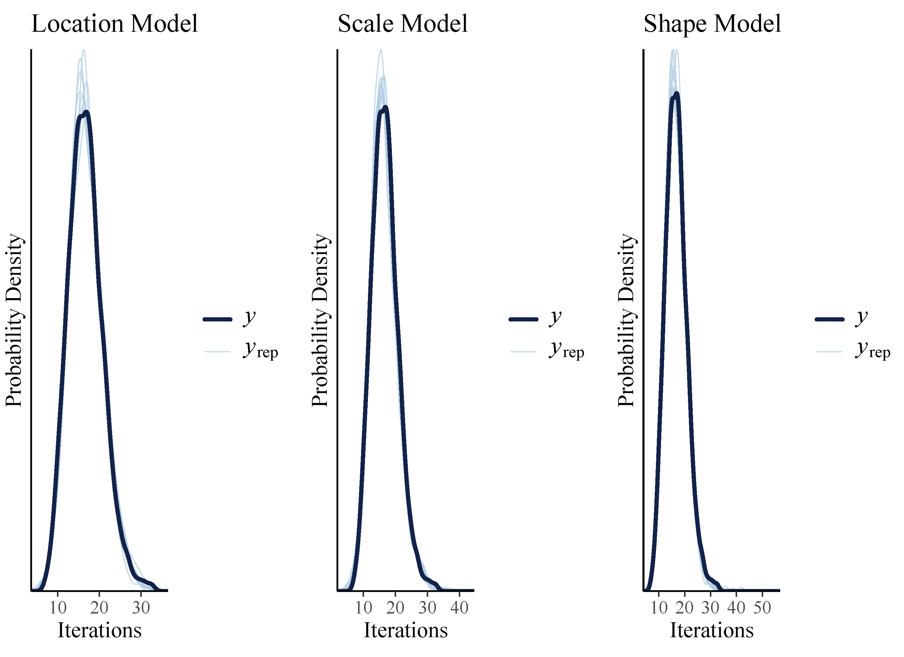
Posterior predctive plots are a way of checking whether the Bayesian models can reproduce the features of the observed data. In the plots, the dark blue lines (y) represents the posterior distribution of the maximum wind speed, while the lighter blue lines () represents the distribution of 10 random draws.
Posterior predictive checks for Kimberley shows weaker fit while Upington shows good fit with Location captured well. Upington seems to be more reliable compared to Kimberley.
Figure 5.
Kimberley Posterior Predictive checks.
3.3.5. Return Levels
Table 16 displays the predicted return levels of daily maximum wind speed across selected return periods and their corresponding 95% confidence intervals indicated in parentheses.
The Bayesian method provides slightly higher estimates, the results in the table shows the return levels increase as the periods increase. Kimberley has the lowest 10 year return level of 21.44 km/h with a narrow confidence interval ranging from 21.18 km/h to 21.72 km/h and Upington has 30.63 km/h return level with a confidence interval ranging from 30.12 km/h to 31.19 km/h. This suggests that a maximum wind speed of 21.44 km/h is expected to increase atleast once in 10 years. 39.85 km/h maximum wind speeds are expected to increase atleast once in 100 years in Upington and 26.52 km/h in Kimberley. From the table, it is clear that Upinton will experience more increase in the wind speed along the years as compared to Kimberly.
The Figure 7, below depicts the return levels plots for the stations.
3.4. Frequentist and Bayesian Performance Comparison
The tables below, Table 17 and Table 18, present the comparison of frequentist and Bayesian metrics (in parantheses). The in-sample performance comparison between the frequentist and Bayesian models show that both approaches deliver similar results with slight differences in the metrics and stations. The Bayesian metrics show lower values compared to the frequentist. For RMSE and MAE, the Bayesian models achieved lower values across all models and stations both for the in-sample and out-of-sample performances. However, for the MAPE, the frequetist achieved lower values in the in-sample performance compared to the out-of-sample.
The out-of-sample performance across all metrics show the Bayesian models to be more powerful than the frequestist. Overall, the results of this paper shows the Bayesian method performs better than the frequentist method for the data used to train the models and also to better to test the models.
Figure 6.
Upington Posterior Predictive checks.
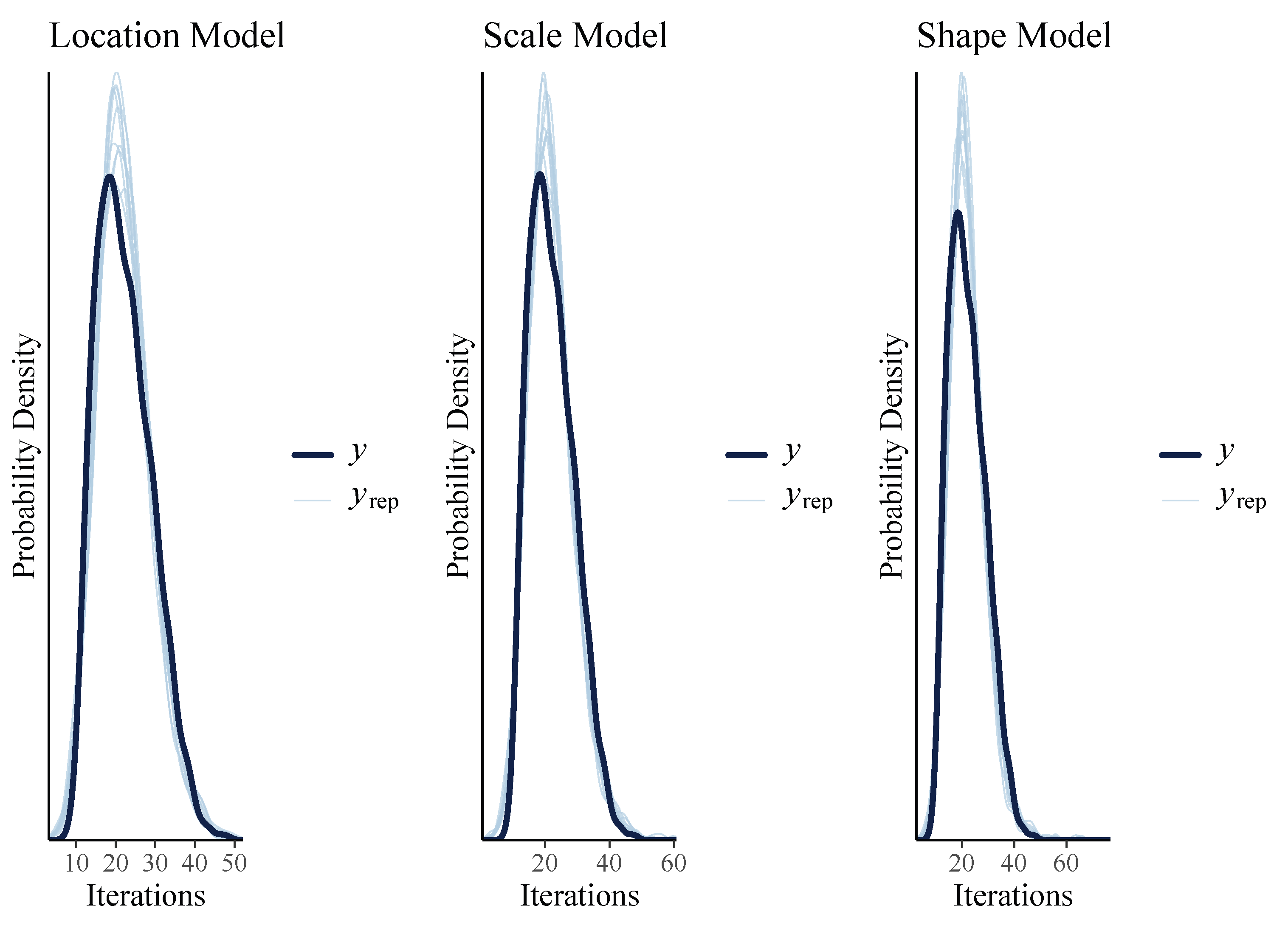
Figure 7.
Return Level plots.
4. Conclusion
Extreme wind speed events have significant impacts on infrastructure, human livelihoods, the economy and agriculture in South Africa. This paper presented a statistical analysis of daily maximum wind speed in a semi-arid region using both frequentist and Bayesian Generalised Additive Extreme Value (GAEV) models. The data were first tested for stationarity using Augmented Dickey-Fuller (ADF), Phillips-Perron (PP) and Kwiatkowski-Phillips-Schmidt-Shin (KPSS) tests, all of which revealed that the series was stationary, which confirmed that the raw series were suitable for extreme value analysis. Although the raw series showed stationary, the inclusion of covariates (seasonality, maximum temperature, maximum relative humidity, and maximum cloud cover) in the GAEV framework explicitly allowed for non-stationary behaviour in the extremes, therefore, capturing climatological drivers of variability. The normality was then assessed using the SW and JB tests where the results revealed that the data were not normally distributed.
Model selection was evaluated using the Akaike Information Criterion (AIC), Bayesian Information Criterion (BIC), and Leave-One-Out Cross-Validation (LOO-CV). For forecasting, Root Mean Squared Error (RMSE), Mean Absolute Error (MAE), and Mean Absolute Percentage Error (MAPE) were applied to check the performance of the models. Across the considered model specifications, the Location model provided the best overall fit and predictive performance according to these criteria, outperforming the Scale and Shape models.
For the return level estimates, the Bayesian framework produced narrower credible intervals, which account for the uncertainties in the return estimates. This suggest that the return estimates are reliable for decision making. The Location model incorporated day of year (seasonality), maximum temperature, maximum relative humidity, and maximum cloud cover as covariates. The results showed that seasonal cycles and temperature are the most influential drivers of extreme wind speed behaviour, while humidity and cloud cover had less significant effects. These results show the significance of seasonal and thermal dynamics in influencing wind extremes and offer useful climatological insights for semi-arid regions.
Overall, the findings demonstrated that the Bayesian GAEV model outperformed the frequentist GAEV model, particularly in terms of predictive accuracy. Therefore, the study concludes that the Bayesian GAEV framework provides a more effective approach to modelling and forecasting daily maximum wind speed extremes at the Kimberley and Upington stations. Despite the findings of this paper, few limitations were encountered, using secondary historical weather data from 2019–2024, which provided short observations and limited the ability to capture long-term climate variability and rare extreme wind speed events, there is limited literature on the modelling of extreme events using frequentist and Bayesian GAEV approaches, making direct comparisons with previous studies challenging.
Future research should extend the study period beyond 2019–2024 and include additional weather stations in all South African provinces to better capture long-term variability and rare extreme events, incorporate additional atmospheric and land-surface variables to improve model performance. Finally, integrating the Generalised Pareto Distribution (GPD) within a Bayesian additive modelling framework using threshold exceedance methods would provide further insight into high-frequency extreme wind speed events. Furthermore, future works should consider probabilistic scoring rules or tail-focused measures such as the quantile score for the 95th percentile, to evaluate tail performance.
Author Contributions
Methodology, T.R. and A.A.; software, M.M.; validation, T.R., A.A., and C.C.; formal analysis, M.M.; investigation, M.M.; data curation, M.M. and C.S.; writing—original draft preparation, M.M. and C.S.; writing—review and editing, T.R., A.A., and C.S.; supervision, T.R., A.A., and C.S.
Funding
This study did not receive direct financial support.
Data Availability Statement
The historical weather data used in this paper were obtained from the Historical Weather API, available at https://open-meteo.com/en/docs/historical-weather-api.
Conflicts of Interest
The authors declare no conflict of interest.
Acknowledgments
The ideas underpinning this work originated from a project by the third author, Albert Antwi, which was funded by the Arid Region Water Research Centre (ARWRC) at Sol Plaatje University. The authors also gratefully acknowledge the support provided by their respective institutions.
Appendix A
Figure A1.
Location model: Kimberley
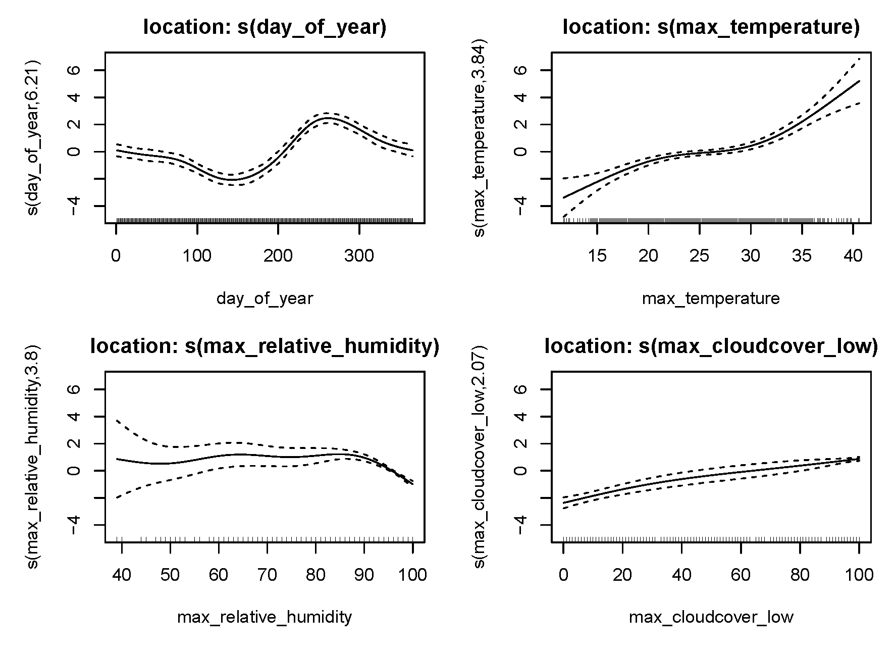
Figure A2.
Scale model: Kimberley
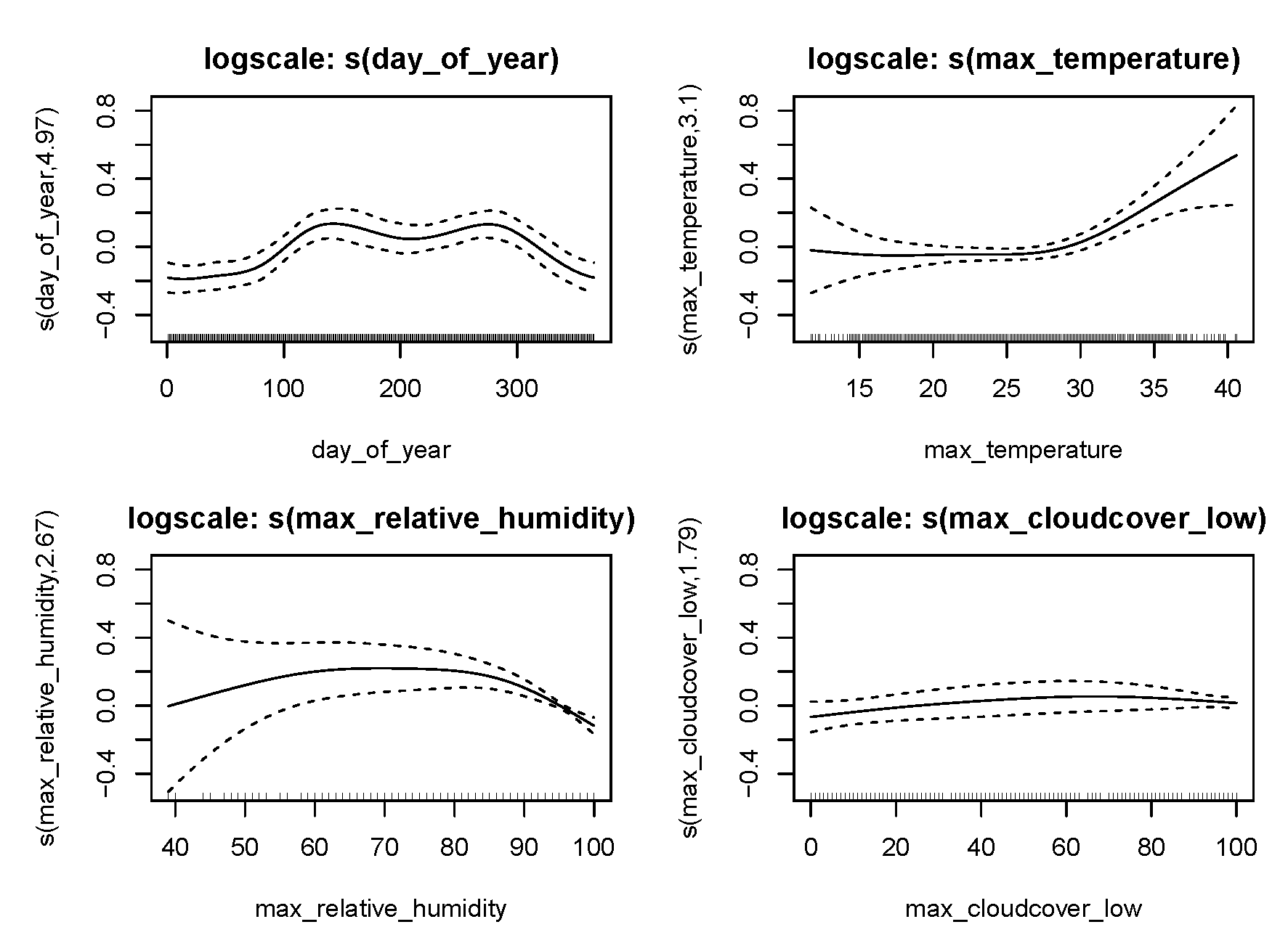
Figure A3.
Shape model: Kimberley
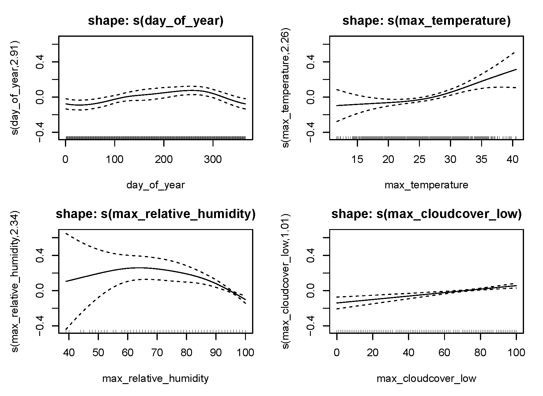
Figure A4.
Location model: Upington
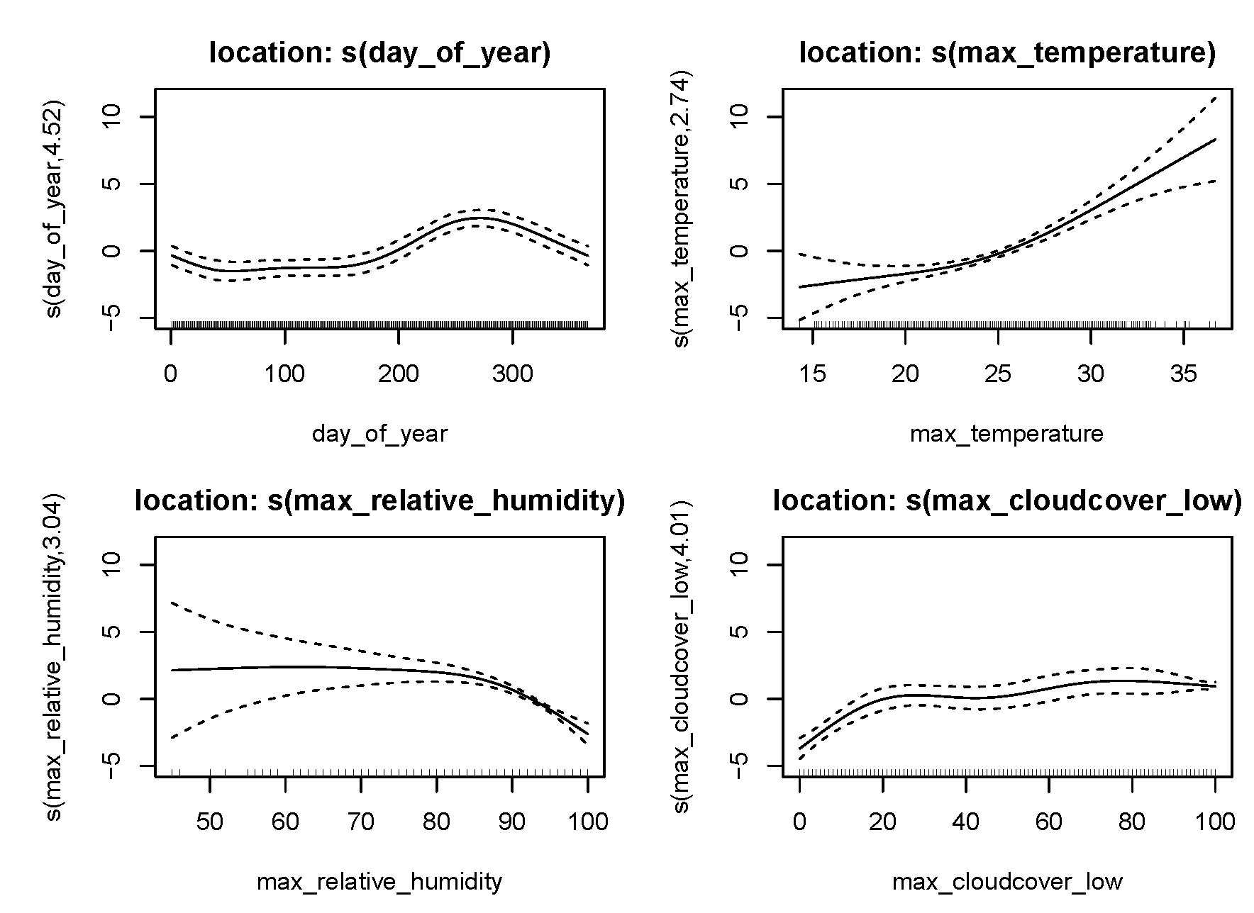
Figure A5.
Scale model: Upington
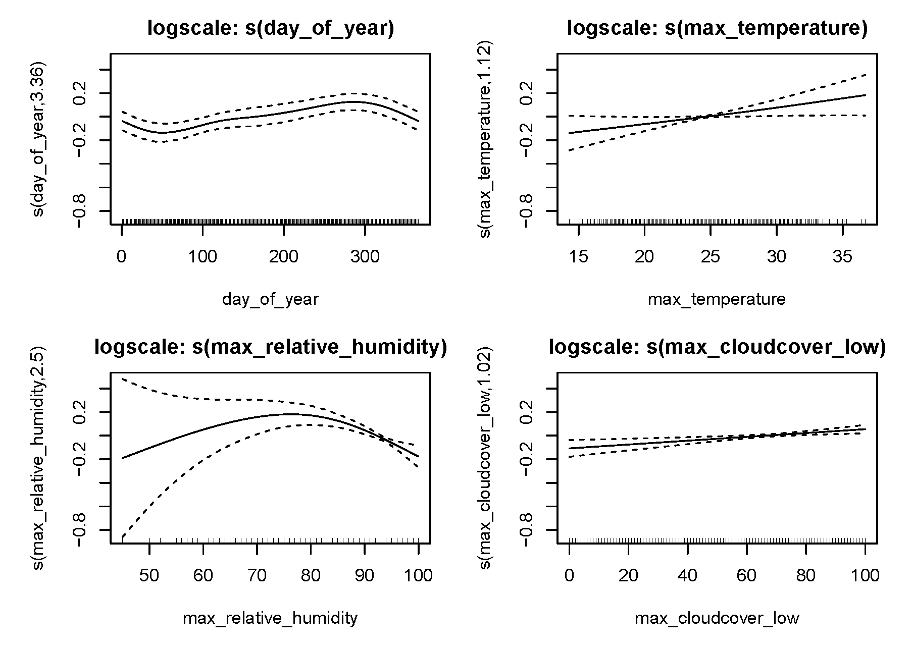
Figure A6.
Shape model: Upington
References
- Herring, D. What is an “extreme event”? Is there evidence that global warming has caused or contributed to any particular extreme event? 2020. Available online: https://www.climate.gov/news-features/climate-qa/what-extreme-event-there-evidence-global-warming-has-caused-or-contributed (accessed on 2024-11-16).
- Rypkema, D.; Tuljapurkar, S. Modeling extreme climatic events using the generalized extreme value (GEV) distribution. In Data Science: Theory and Applications;Handbook of Statistics; Rao, Srinivasa, Rao, A.S.C., Eds.; Elsevier, 2021; Vol. 44, pp. 39–71. [Google Scholar] [CrossRef]
- Philippe, N.; Alexis, H.; Aurélien, R. Statistical Methods for Extreme Event Attribution in Climate Science. Annu. Rev. Stat. Its Appl. 2020, 7, 89–110. [Google Scholar] [CrossRef]
- Youngman, B. evgam: An R package for generalized additive extreme value models. J. Stat. Softw. 2022, 103, 1–26. [Google Scholar] [CrossRef]
- Debusho, L.; Diriba, T. Bayesian modelling of summer daily maximum temperature data; 2016; pp. 126–133. [Google Scholar]
- Diriba, T.; Debusho, L. Modelling dependency effect to extreme value distributions with the application to extreme wind at Port Elizabeth, South Africa: a Frequentist and Bayesian approaches. 2020, 35, 1449–1479. [Google Scholar] [CrossRef]
- Antwi, A.; Kammies, E.; Chaka, L.; Arasomwan, M. Forecasting South African grain prices and assessing the non-linear impact of inflation and rainfall using a dynamic Bayesian generalized additive model. Front. Appl. Math. Stat. 2025, 11, 1582609. [Google Scholar] [CrossRef]
- Sathyanarayana, S.; Mohanasundaram, T. Stationarity and unit roots in time series: Theoretical insights and practical considerations. IRA-Int. J. Manag. Soc. Sci. (ISSN 2455-2267) 2025, 21, 46–46. [Google Scholar] [CrossRef]
- Guo, Z. Research on the Augmented Dickey-Fuller Test for Predicting Stock Prices and Returns. Adv. Econ. Manag. Political Sci. 2023, 44, 101–106. [Google Scholar] [CrossRef]
- Petrică, A.; Stancu, S.; Ghițulescu, V. Stationarity–The central concept in time series analysis. Int. J. Emerg. Res. Manag. Technol. 2017, 6, 6–16. [Google Scholar] [CrossRef] [PubMed]
- Salkind, N. Shapiro-wilk test for normality. Encycl. Meas. Stat. 2007, 0, 884–886. [Google Scholar] [CrossRef]
- Abbes, A.; Essid, H.; Farah, I.; Barra, V. Rare events detection in NDVI time-series using Jarque-Bera test; 2015; pp. 338–341. [Google Scholar]
- Masereka, E.; Ochieng, G.; Snyman, J. Statistical analysis of annual maximum daily rainfall for Nelspruit and its environs. Jàmbá J. Disaster Risk Stud. 2018, 10, 1–10. [Google Scholar] [CrossRef] [PubMed]
- Shitu, D.; Ahmed, A.; Ali Muhamed, G.; Abbas, F. Describing Long-Term Trends in temperature of Jos region of Nigeria, using Generalized Additive Models (GAMs). 2024. [Google Scholar] [CrossRef]
- Xiang, D. Fitting generalized additive models with the GAM procedure. In Proceedings of the SUGI Proceedings, Citeseer, 2001; pp. 256–326. [Google Scholar]
- Mashishi, D. Modeling average monthly rainfall for South Africa using extreme value theory. PhD thesis, University of the Limpopo, Faculty of Science and Agriculture, School of Mathematical and Computer Sciences, 2020. [Google Scholar]
- Chikobvu, D.; Chifurira, R. Modelling of extreme minimum rainfall using generalised extreme value distribution for Zimbabwe. South Afr. J. Sci. 2015, 111, 01–08. [Google Scholar] [CrossRef] [PubMed]
- Sikhwari, T. Variability and long-term trends of climate extremes over the Limpopo, South Africa. PhD thesis, University of Vendda, Faculty of Science, Engineering and Agriculture, School of Environmental Sciences, 2019. [Google Scholar]
- Autcha, A.; Paradorn, S. Parameter Estimation For Generalized Extreme Value Distribution In Rainfall Forecasting: A Case Study Of Bangkok. J. Appl. Sci. Eng. 2025, 28, 2409–2426. [Google Scholar]
- Ayitey, E.; Nyarko, C.; Otoo, H.; Affam, M. Extreme Value Theory Modeling of Geochemical Anomalies: Block Maxima Approach. Asian J. Probab. Stat. 2022, 17, 86–95. [Google Scholar] [CrossRef]
- Wasserman, L. Bayesian model selection and model averaging. J. Math. Psychol. 2000, 44, 92–107. [Google Scholar] [CrossRef] [PubMed]
- Gneiting, T.; Wolffram, D.; Resin, J.; Kraus, K.; Bracher, J.; Dimitriadis, T.; Hagenmeyer, V.; Jordan, A.; Lerch, S.; Phipps, K.; et al. Model diagnostics and forecast evaluation for quantiles. Annu. Rev. Stat. Its Appl. 2023, 10, 597–621. [Google Scholar] [CrossRef]
- Iyamuremye, E.; Mung’atu, J.; Mwita, P. Extreme value modelling of rainfall using poisson-generalized pareto distribution: A case study Tanzania. Int. J. Stat. Distrib. Appl. 2019, 5, 67–75. [Google Scholar] [CrossRef]
- Then, J.; Permana, F.; Yong, B. Parameters estimation of lognormal and pareto type distributions using frequentist and bayesian inferences. BAREKENG J. Math. Its Appl. 2025, 19, 141–152. [Google Scholar] [CrossRef]
Figure 1.
Northern Cape Stations.
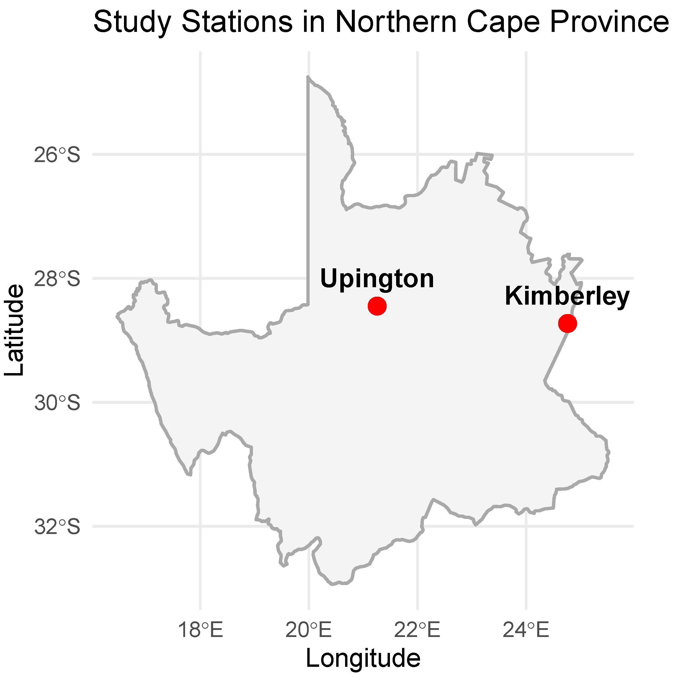
Figure 2.
Diagnostic plots illustrating the fit of the data at Kimberley station.
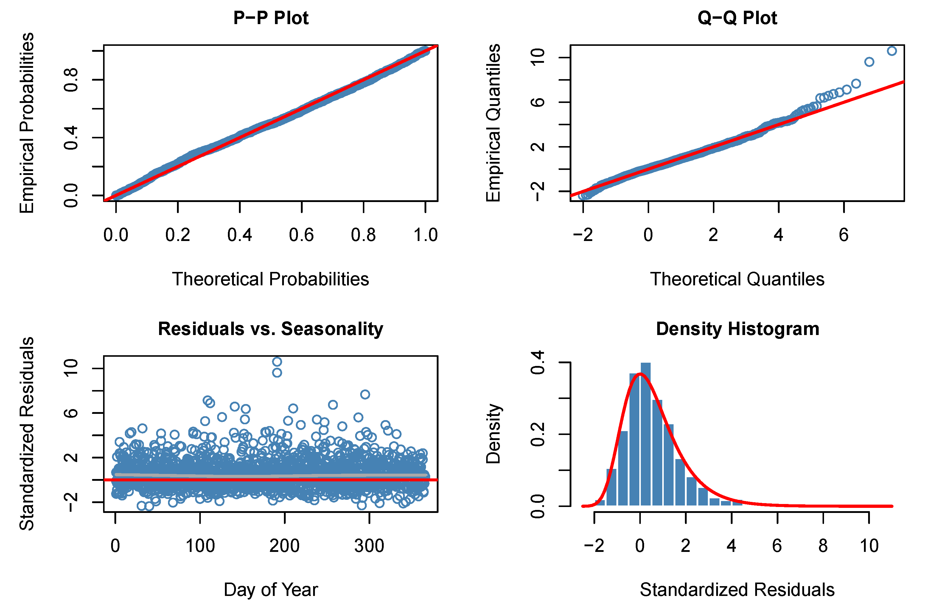
Figure 3.
Diagnostic plots illustrating the fit of the data at Upington station.
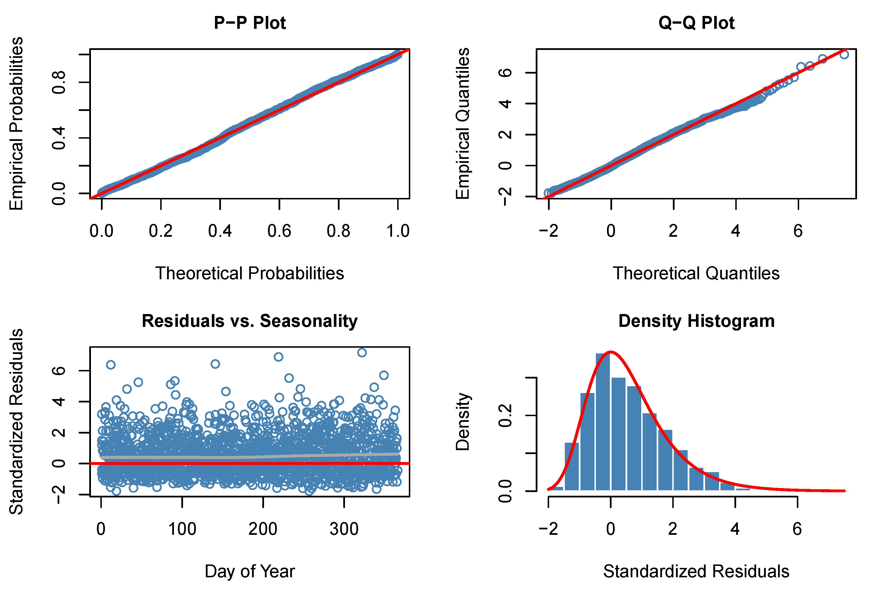
Figure 4.
Return Level plots.
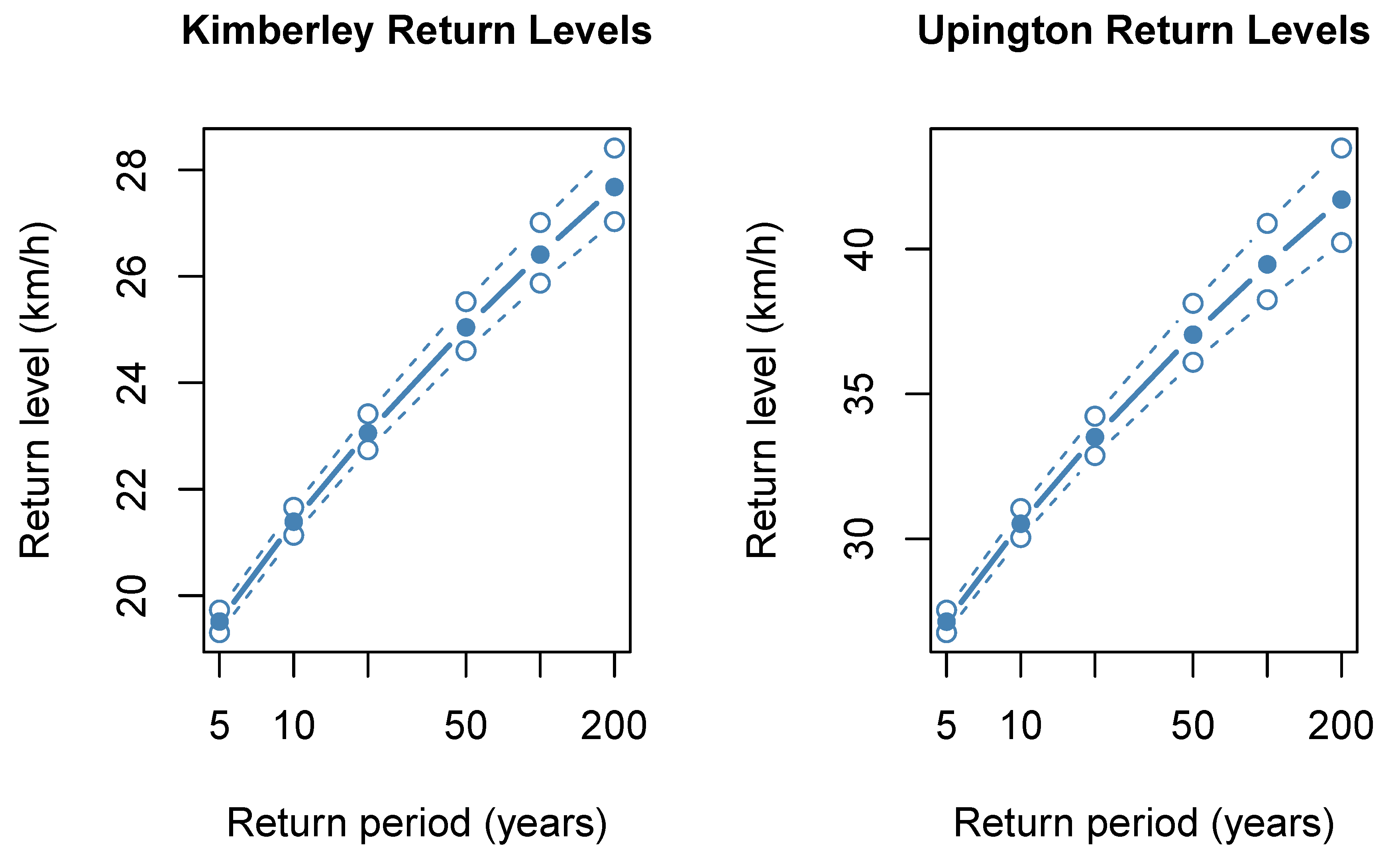

Table 1.
Summary statistics of Kimberly and Upington maximum wind speed.
| Station | Min | Median | Max | Mean | Sd | Skew | Kurt |
|---|---|---|---|---|---|---|---|
| Kimberley | 7.10 | 16.60 | 35.30 | 16.90 | 4.14 | 0.52 | 3.58 |
| Upington | 8.00 | 21.40 | 47.70 | 22.30 | 6.91 | 0.53 | 2.75 |
0.85 Note: Min=Minimum, Max=Maximum, Sd=Standard deviation, Skew=Skewness, Kurt=Kurtosis.
Table 2.
Stationarity test results for daily maximum wind speed.
| Station | ADF | PP | KPSS | |||
|---|---|---|---|---|---|---|
| Statistic | p-value | Statistic | p-value | Statistic | p-value | |
| Kimberley | -6.722 | 0.010 | -1947.60 | 0.010 | 0.293 | 0.010 |
| Upington | -25.021 | 0.010 | -2045.50 | 0.010 | 0.101 | 0.010 |
0.85 Note: KIM = Kimberley, UPT = Upington.
Table 3.
Normality test results for daily maximum wind speed.
| Station | S-W | J-B | ||
|---|---|---|---|---|
| Statistic | p-value | Statistic | p-value | |
| Kimberley | 0.985 | 131.040 | ||
| Upington | 0.972 | 107.980 | ||
Table 4.
Parametric intercept estimates for GEV parameters.
| Model | Intercepts | KIM | UPT |
|---|---|---|---|
| Location | 15.30 (0.08) | 19.50 (0.15) | |
| 1.11 (0.02) | 1.71 (0.02) | ||
| -0.10 (0.01) | -0.11 (0.02) | ||
| Scale | 15.09 (0.11) | 18.93 (0.17) | |
| 1.31 (0.02) | 1.78 (0.02) | ||
| -0.18 (0.02) | -0.12 (0.02) | ||
| Shape | 15.01 (0.1) | 19.14 (0.16) | |
| 1.28 (0.02) | 1.74 (0.02) | ||
| -0.18 (0.02) | -0.10 (0.02) |
0.85 Note: KIM = Kimberley, UPT = Upington.
Table 5.
Smooth Terms: Kimberley.
| Model | Smooth terms | edf | Chi-square | p-value | |
|---|---|---|---|---|---|
| Location | s(day_of_year) | 6.21 | 323.20 | <2e-16 | |
| s(max_temperature) | 3.84 | 124.44 | <2e-16 | ||
| s(max_relative_humidity) | 3.80 | 68.41 | 5.37e-14 | ||
| s(max_cloudcover) | 2.07 | 155.26 | <2e-16 | ||
| Scale | s(day_of_year) | 4.97 | 42.48 | 3.19e-08 | |
| s(max_temperature) | 3.10 | 27.22 | 6.95e-06 | ||
| s(max_relative_humidity) | 2.67 | 26.87 | 1.15e-05 | ||
| s(max_cloudcover) | 1.79 | 3.49 | 0.246 | ||
| Shape | s(day_of_year) | 2.91 | 12.66 | 0.003 | |
| s(max_temperature) | 2.26 | 23.36 | 3.66e-05 | ||
| s(max_relative_humidity) | 2.34 | 27.52 | 3.57e-06 | ||
| s(max_cloudcover) | 1.01 | 17.50 | 2.93e-05 |
Table 6.
Smooth Terms: Upington.
| Model | Smooth terms | edf | Chi-square | p-value | |
|---|---|---|---|---|---|
| Location | s(day_of_year) | 4.52 | 94.10 | <2e-16 | |
| s(max_temperature) | 2.74 | 81.57 | <2e-16 | ||
| s(max_relative_humidity) | 3.04 | 63.17 | 1.48e-13 | ||
| s(max_cloudcover) | 4.01 | 95.91 | <2e-16 | ||
| Scale | s(day_of_year) | 3.36 | 19.80 | 0.000 | |
| s(max_temperature) | 1.12 | 5.00 | 0.037 | ||
| s(max_relative_humidity) | 2.50 | 23.42 | 2.06e-05 | ||
| s(max_cloudcover) | 1.02 | 9.33 | 0.002 | ||
| Shape | s(day_of_year) | 1.81 | 5.35 | 0.041 | |
| s(max_temperature) | 1.05 | 0.60 | 0.461 | ||
| s(max_relative_humidity) | 1.02 | 8.12 | 0.004 | ||
| s(max_cloudcover) | 1.03 | 15.97 | 7.05e-05 |
Table 7.
Goodness-of-fit Test Results Using MLE Parameters.
| Stations | Metrics | Model | ||
|---|---|---|---|---|
| Location | Scale | Shape | ||
| KIM | K-S | 0.0317 | 0.0192 | 0.0288 |
| p-value | 0.0597 | 0.5347 | 0.1809 | |
| A-D | 2.2962 | 0.4478 | 1.2608 | |
| p-value | 0.0635 | 0.8003 | 0.2455 | |
| UPT | K-S | 0.0260 | 0.0440 | 0.0456 |
| p-value | 0.1865 | 0.0023 | 0.0014 | |
| A-D | 1.6769 | 4.0611 | 5.7237 | |
| p-value | 0.1394 | 0.0081 | 0.0013 | |
0.85 Note: KIM = Kimberley, UPT = Upington.
Table 8.
Model Selection for Location, Scale, and Shape Models.
| Stations | Metrics | Model | ||
|---|---|---|---|---|
| Location | Scale | Shape | ||
| KIM | AIC | 9223.35 | 9784.94 | 9832.29 |
| BIC | 9326.85 | 9869.85 | 9895.28 | |
| UPT | AIC | 11363.51 | 11590.65 | 11609.70 |
| BIC | 11458.14 | 11650.86 | 11653.01 | |
0.85 Note: KIM = Kimberley, UPT = Upington.
Table 9.
Metrics Evaluation for In-sample and Out-of-sample Performance.
| Station & Metric | In-sample | Out-of-sample | |||||
|---|---|---|---|---|---|---|---|
| Location | Scale | Shape | Location | Scale | Shape | ||
| KIM | RMSE | 3.71 | 4.45 | 4.48 | 5.18 | 4.72 | 4.76 |
| MAE | 2.75 | 3.43 | 3.46 | 4.07 | 3.61 | 3.65 | |
| MAPE | 15.87 | 20.20 | 20.25 | 22.97 | 19.75 | 19.87 | |
| UPT | RMSE | 6.83 | 7.62 | 7.54 | 8.01 | 7.89 | 7.79 |
| MAE | 5.34 | 5.91 | 5.86 | 6.33 | 6.18 | 6.11 | |
| MAPE | 23.42 | 25.56 | 25.57 | 27.33 | 25.76 | 25.71 | |
0.85 Note: KIM = Kimberley, UPT = Upington.
Table 10.
Estimated return years and levels (km/h).
| Return Years | KIM | UPT |
|---|---|---|
| 5 years | 19.30 (19.30, 19.73) | 27.14 (26.76, 27.54) |
| 10 years | 21.39 (21.14, 21.66) | 30.52 (30.04, 31.04) |
| 20 years | 23.06 (22.74, 23.42) | 33.51 (32.87, 34.23) |
| 50 years | 25.04 (24.60, 25.53) | 37.05 (36.09, 38.13) |
| 100 years | 26.41 (25.87, 27.01) | 39.47 (38.25, 40.88) |
| 200 years | 27.68 (27.03, 28.41) | 1.71 (40.22, 43.48) |
Table 11.
Bayesian GAEV convergence estimates for the models; Location, Scale, and Shape: Kimberley.
Table 11.
Bayesian GAEV convergence estimates for the models; Location, Scale, and Shape: Kimberley.
| Model | Parameter | Rhat | Bulk ESS | Tail ESS |
|---|---|---|---|---|
| Smoothing Spline Hyperparameters | ||||
| Location | Day of Year | 1.00 | 1849 | 3856 |
| Temperature | 1.00 | 3249 | 1967 | |
| Relative Humidity | 1.00 | 5918 | 4926 | |
| Cloudcover | 1.00 | 2956 | 3088 | |
| Scale | Day of Year | 1.00 | 1299 | 1933 |
| Temperature | 1.00 | 2547 | 3936 | |
| Relative Humidity | 1.00 | 2878 | 2104 | |
| Cloudcover | 1.00 | 1777 | 1022 | |
| Shape | Day of Year | 1.00 | 637 | 1034 |
| Temperature | 1.00 | 984 | 793 | |
| Relative Humidity | 1.00 | 1589 | 1434 | |
| Cloudcover | 1.00 | 1073 | 1029 | |
| Regression Coefficients | ||||
| Location | Intercept | 1.00 | 10533 | 6097 |
| Sigma intercept | 1.00 | 10288 | 6225 | |
| Shape intercept | 1.00 | 9584 | 6110 | |
| Temperature | 1.00 | 5673 | 5302 | |
| Relative Humidity | 1.00 | 9671 | 5285 | |
| Cloudcover | 1.00 | 4051 | 4593 | |
| Scale | Intercept | 1.00 | 5549 | 1783 |
| Sigma intercept | 1.00 | 4348 | 1861 | |
| Shape intercept | 1.00 | 5130 | 5402 | |
| Temperature | 1.00 | 3160 | 1327 | |
| Relative Humidity | 1.00 | 4594 | 5367 | |
| Cloudcover | 1.00 | 2992 | 2392 | |
| Shape | Intercept | 1.00 | 2287 | 1346 |
| Sigma intercept | 1.00 | 2125 | 1392 | |
| Shape intercept | 1.00 | 1430 | 1552 | |
| Temperature | 1.00 | 1820 | 1663 | |
| Relative Humidity | 1.00 | 2321 | 1528 | |
| Cloudcover | 1.00 | 1792 | 1458 |
Table 12.
Bayesian GAEV convergence estimates for the models; Location, Scale, and Shape: Upington.
| Model | Parameter | Rhat | Bulk ESS | Tail ESS |
|---|---|---|---|---|
| Smoothing Spline Hyperparameters | ||||
| Location | Day of Year | 1.00 | 2339 | 3367 |
| Temperature | 1.00 | 5330 | 4939 | |
| Relative Humidity | 1.00 | 7988 | 5632 | |
| Cloudcover | 1.00 | 5644 | 4693 | |
| Scale | Day of Year | 1.00 | 1576 | 1518 |
| Temperature | 1.00 | 2622 | 3448 | |
| Relative Humidity | 1.00 | 3541 | 2573 | |
| Cloudcover | 1.00 | 1704 | 1296 | |
| Shape | Day of Year | 1.00 | 979 | 677 |
| Temperature | 1.00 | 1042 | 924 | |
| Relative Humidity | 1.00 | 1167 | 694 | |
| Cloudcover | 1.00 | 1004 | 706 | |
| Regression Coefficients | ||||
| Location | Intercept | 1.00 | 10070 | 6214 |
| Sigma intercept | 1.00 | 10048 | 6089 | |
| Shape intercept | 1.00 | 8937 | 6508 | |
| Temperature | 1.00 | 10739 | 5713 | |
| Relative Humidity | 1.00 | 8703 | 6665 | |
| Cloudcover | 1.00 | 11073 | 5266 | |
| Scale | Intercept | 1.00 | 8641 | 5548 |
| Sigma intercept | 1.00 | 7741 | 5630 | |
| Shape intercept | 1.00 | 7423 | 6280 | |
| Temperature | 1.00 | 4786 | 4171 | |
| Relative Humidity | 1.00 | 6245 | 5813 | |
| Cloudcover | 1.00 | 2793 | 2184 | |
| Shape | Intercept | 1.00 | 3125 | 1358 |
| Sigma intercept | 1.00 | 2538 | 1536 | |
| Shape intercept | 1.00 | 2375 | 1690 | |
| Temperature | 1.00 | 3627 | 1389 | |
| Relative Humidity | 1.00 | 3091 | 1319 | |
| Cloudcover | 1.00 | 2170 | 1440 |
Table 13.
Goodness-of-fit test results for extreme GAMs.
| Stations | Metrics | Model | ||
|---|---|---|---|---|
| Location | Scale | Shape | ||
| KIM | K-S | 0.032 | 0.019 | 0.027 |
| p-value | 0.056 | 0.549 | 0.143 | |
| A-D | 2.454 | 0.521 | 1.080 | |
| p-value | 0.052 | 0.725 | 0.318 | |
| UPT | K-S | 0.027 | 0.042 | 0.042 |
| p-value | 0.168 | 0.005 | 0.004 | |
| A-D | 1.892 | 3.956 | 5.266 | |
| p-value | 0.105 | 0.009 | 0.002 | |
0.85 Note: KIM = Kimberley, UPT = Upington.
Table 14.
LOO-CV tests.
| Model | Station | elpd_loo | p_loo | looic | Pareto estimates |
|---|---|---|---|---|---|
| Location | KIM | -4617.5 (35.0) | 21.3 (1.7) | 9234.9 (70.1) | k<0.7 |
| UPT | -5789.8 (27.3) | 10.7 (0.7) | 11367.7 (54.7) | k<0.7 | |
| Scale | KIM | -4888.2 (30.6) | 17.6 (1.8) | 10777.1 (61.3) | k<0.7 |
| UPT | -5789.9 (27.3) | 10.7 (0.7) | 11579.8 (54.5) | k<0.7 | |
| Shape | KIM | -4913.7 (29.7) | 10.0 (1.7) | 9827.5 (59.5) | k<0.7 |
| UPT | -5799.4 (27.5) | 6.1 (0.7) | 11598.6 (54.8) | k<0.7 |
0.85 Note: KIM = Kimberley, UPT = Upington.
Table 15.
Metrics Evaluation for In-sample and Out-of-sample Performance.
| Station & Metric | In-sample | Out-of-sample | |||||
|---|---|---|---|---|---|---|---|
| Location | Scale | Shape | Location | Scale | Shape | ||
| KIM | RMSE | 3.44 | 4.10 | 4.05 | 3.82 | 4.17 | 4.15 |
| MAE | 2.64 | 3.23 | 3.19 | 2.86 | 3.22 | 3.21 | |
| MAPE | 16.73 | 21.06 | 20.59 | 17.04 | 19.29 | 19.03 | |
| UPT | RMSE | 6.33 | 6.81 | 6.78 | 6.69 | 6.92 | 6.90 |
| MAE | 5.16 | 5.55 | 5.55 | 5.51 | 5.63 | 5.64 | |
| MAPE | 25.72 | 27.45 | 27.70 | 27.18 | 26.82 | 27.14 | |
0.85 Note: KIM = Kimberley, UPT = Upington.
Table 16.
Estimated return years and levels (km/h).
| Stations | ||
|---|---|---|
| Return Periods | KIM | UPT |
| 5 years | 19.55 (19.33, 19.77) | 27.18 (26.77, 27.61) |
| 10 years | 21.44 (21.18, 21.72) | 30.63 (30.12, 31.19) |
| 20 years | 23.13 (22.80, 23.49) | 33.69 (33.02, 34.46) |
| 50 years | 25.13 (24.70, 25.63) | 37.34 (36.37, 38.51) |
| 100 years | 26.52 (25.98, 27.15) | 39.85 (38.60, 41.40) |
| 200 years | 27.80 (27.15, 28.57) | 42.18 (40.62, 44.17) |
Table 17.
Metrics Evaluation (in-sample Performance).
| Stations | Metrics | Model | ||
|---|---|---|---|---|
| Location | Scale | Shape | ||
| KIM | RMSE | 3.71 (3.44) | 4.45 (4.10) | 4.48 (4.05) |
| MAE | 2.75 (2.64) | 3.43 (3.23) | 3.46 (3.19) | |
| MAPE | 15.87 (16.73) | 20.20 (21.06) | 20.25 (20.59) | |
| UPT | RMSE | 6.83 (6.33) | 7.62 (6.81) | 7.54 (6.78) |
| MAE | 5.34 (5.16) | 5.91 (5.55) | 5.86 (5.55) | |
| MAPE | 23.42 (25.72) | 25.56 (27.45) | 25.57 (27.70) | |
0.85 Note: KIM = Kimberley, UPT = Upington.
Table 18.
Metrics Evaluation (out-of-sample Performance).
| Stations | Metrics | Model | ||
|---|---|---|---|---|
| Location | Scale | Shape | ||
| KIM | RMSE | 5.18 (3.82) | 4.72 (4.17) | 4.76 (4.15) |
| MAE | 4.07 (2.86) | 3.61 (3.22) | 3.65 (3.21) | |
| MAPE | 22.97 (17.04) | 19.75 (19.29) | 19.87 (19.03) | |
| UPT | RMSE | 8.01 (6.69) | 7.89 (6.92) | 7.79 (6.90) |
| MAE | 6.33 (5.51) | 6.18 (5.63) | 6.11 (5.64) | |
| MAPE | 27.33 (27.18) | 25.76 (26.82) | 25.71 (27.14) | |
0.85 Note: KIM = Kimberley, UPT = Upington.
Disclaimer/Publisher’s Note: The statements, opinions and data contained in all publications are solely those of the individual author(s) and contributor(s) and not of MDPI and/or the editor(s). MDPI and/or the editor(s) disclaim responsibility for any injury to people or property resulting from any ideas, methods, instructions or products referred to in the content. |
© 2026 by the authors. Licensee MDPI, Basel, Switzerland. This article is an open access article distributed under the terms and conditions of the Creative Commons Attribution (CC BY) license (http://creativecommons.org/licenses/by/4.0/).
Copyright: This open access article is published under a Creative Commons CC BY 4.0 license, which permit the free download, distribution, and reuse, provided that the author and preprint are cited in any reuse.