Toward a Unified Mathematical Theory of Neuroanesthesia: Integrating Algebra, Differential Calculus, and Neural Network Dynamics—Introducing the Unified Neuroanesthesia Neural Index (UNNI): A Theoretical Computational Framework for Modeling Brain Stability During Anesthesia

1. Introduction

1.1. The Brain as a Complex Dynamic System During Neuroanesthesia

The central nervous system represents one of the most complex biological networks known in medicine. During anesthesia, neuronal communication is progressively altered through mechanisms involving synaptic inhibition, changes in neurotransmitter activity, modifications of cortical oscillations, and alterations in cerebral metabolism.

Unlike simple physical systems, the brain does not respond linearly to external stimulation. Small changes in anesthetic concentration may produce significant modifications in consciousness, electrical activity, and physiological regulation. This behavior suggests that neuroanesthesia should be analyzed using mathematical approaches capable of describing nonlinear and time-dependent systems.

A major challenge in neuroanesthesia is the absence of a unified model capable of integrating neural electrical activity, pharmacological anesthetic effects, cerebral oxygen metabolism, hemodynamic regulation, and functional connectivity. The proposed UNNI framework attempts to mathematically represent these interacting domains.

Mathematical Model 1 — Neurophysiological State Vector

The brain during anesthesia is represented as a multidimensional vector combining five physiological dimensions into a unified mathematical space, rather than evaluating each parameter in isolation.

$$X\left(t\right)={\left[,N,\left(t\right),,A\left(t\right)H\left(t\right)M\left(t\right)C\left(t\right)\right]}^T$$

Equation (1) — neurophysiological state vector

Where N(t) is neuronal function, A(t) is anesthetic influence, H(t) is vascular and cardiovascular regulation, M(t) is metabolic activity, and C(t) is connectivity state.

Figure 1. Conceptual dynamic model of the Unified Neuroanesthesia Neural Index (UNNI).

Figure 1. Conceptual dynamic model of the Unified Neuroanesthesia Neural Index (UNNI).

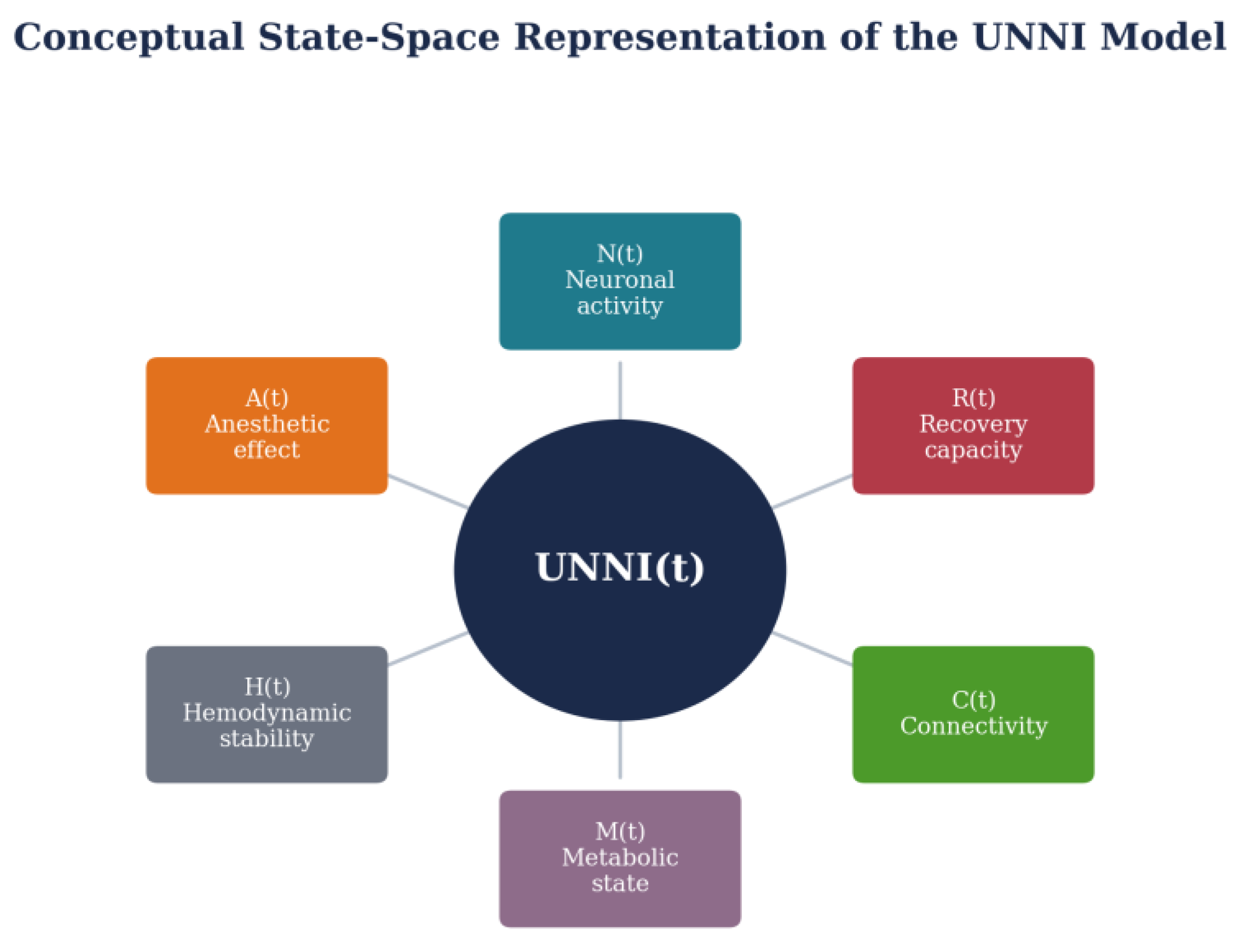
Interaction between anesthetic administration, neuronal activity, cerebral metabolism, hemodynamic regulation, and neural connectivity over time.

Table 2. Major physiological components incorporated into the UNNI model.

Variable	Mathematical Representation	Biological Meaning
N(t)	Neural activity function	Electrical brain activity
A(t)	Drug-response function	Anesthetic influence
H(t)	Hemodynamic function	Cerebral perfusion stability
M(t)	Metabolic function	Energy consumption
C(t)	Connectivity function	Neural network organization

Table 2. Major physiological components incorporated into the UNNI model.

Variable	Mathematical Representation	Biological Meaning
N(t)	Neural activity function	Electrical brain activity
A(t)	Drug-response function	Anesthetic influence
H(t)	Hemodynamic function	Cerebral perfusion stability
M(t)	Metabolic function	Energy consumption
C(t)	Connectivity function	Neural network organization

The Proposed UNNI Equation

Building on the state vector above, the theoretical index integrating instantaneous physiological state and accumulated physiological history is expressed as:

$$\mathrm{U}\mathrm{N}\mathrm{N}\mathrm{I}\left(t\right)=\sum _{i=1}^n{w}_i{X}_i\left(t\right)+\lambda {\int }_0^{t}F\left(X\left(\tau \right)\right)d\tau$$

Equation (2) — the proposed UNNI equation

Where w_i represents the contribution weight of each physiological component, X_i(t) represents individual neurophysiological variables, λ represents a temporal integration coefficient, and F(X) represents nonlinear interaction between physiological variables. The first term, Σw_iX_i(t), represents the instantaneous physiological state; the second term, λ∫F(X(τ))dτ, represents the accumulated effect of previous physiological changes, reflecting the memory characteristics of biological systems. This equation proposes that neuroanesthetic stability is not determined by a single measurement but emerges from the interaction of multiple biological systems over time.

Mathematical Model 2 — Differential Evolution of Brain State

$${\displaystyle \frac{dX\left(t\right)}{dt}}=f\left(X,\left(t\right),u\left(t\right)\theta \right)$$

Equation (3) — differential evolution of the neurological state

Where u(t) is the anesthetic input function, θ represents biological parameters, and f is a nonlinear transformation function. This differential equation describes how the neurological state changes with time: increasing anesthetic concentration modifies u(t), producing changes in neuronal activity and connectivity.

Mathematical Model 3 — Weighted Physiological Integration

$$S\left(t\right)=w_{N}N\left(t\right)+w_{A}A\left(t\right)+w_{H}H\left(t\right)+w_{M}M\left(t\right)+w_{C}C\left(t\right)$$

Equation (4) — weighted physiological integration

Not every physiological variable contributes equally. Neuronal activity may carry a higher weight during deep anesthesia monitoring, whereas hemodynamic variables may dominate during cardiovascular instability.

Mathematical Model 4 — Nonlinear Interaction Function

$$F\left(X\right)=\alpha N\left(t\right)A\left(t\right)+\beta H\left(t\right)M\left(t\right)+\gamma C{\left(t\right)}^2$$

Equation (5) — nonlinear interaction between physiological components

The term N(t)A(t) represents the relationship between neuronal activity and anesthetic effect; H(t)M(t) represents the interaction between blood flow and metabolism; and C(t)² represents nonlinear amplification of connectivity changes.

1.2. Mathematical Representation of Neuroanesthetic Stability and Nonlinear Brain Dynamics

The physiological state of the brain during anesthesia cannot be considered a static condition. Instead, it represents a continuously evolving dynamic system influenced by pharmacological interventions, internal biological regulation, and external physiological disturbances.

In mathematical terms, the anesthetized brain can be represented as a nonlinear dynamical system where the current state depends not only on present variables but also on previous physiological conditions:

$$X\left(t+\Delta t\right)=X\left(t\right)+\Delta X\left(t\right)$$

Equation (6) — discrete-time state evolution

where X(t) represents the current neurophysiological state, X(t+Δt) represents the future state, and ΔX(t) represents the physiological change occurring during a defined time interval. This fundamental concept allows the UNNI framework to describe anesthesia as a continuous trajectory rather than a single measurement.

Mathematical Model 5 — Dynamic Stability Equation

$${\displaystyle \frac{dS\left(t\right)}{dt}}={\displaystyle \frac{\partial S}{\partial N}}{\displaystyle \frac{dN}{dt}}+{\displaystyle \frac{\partial S}{\partial A}}{\displaystyle \frac{dA}{dt}}+{\displaystyle \frac{\partial S}{\partial H}}{\displaystyle \frac{dH}{dt}}+{\displaystyle \frac{\partial S}{\partial M}}{\displaystyle \frac{dM}{dt}}$$

Equation (7) — sensitivity-weighted rate of change of stability

This equation applies differential calculus to evaluate how neuroanesthetic stability changes over time. The total change in stability S(t) depends on the rate of change of neuronal activity N(t), anesthetic concentration A(t), hemodynamic status H(t), and metabolic condition M(t). The partial derivatives describe the sensitivity of the stability index to each physiological component — for example, ∂S/∂A represents how strongly anesthetic changes influence overall neurophysiological stability.

A rapid increase in anesthetic concentration (dA/dt > 0) may lead to dN/dt < 0 as neuronal activity decreases; however, the final effect on UNNI depends on the interaction between all variables, not anesthesia alone — reflecting the complexity of biological systems.

Mathematical Model 6 — Integral Representation of Cumulative Anesthetic Effect

$$E_A\left(t\right)={\int }_0^{t}A\left(\tau \right)K\left(t-\tau \right)d\tau$$

Equation (8) — cumulative anesthetic effect

Where E_A(t) is the cumulative anesthetic effect, A(τ) is anesthetic concentration at previous time points, and K(t−τ) is a biological response function representing the delay between drug administration and physiological response. Anesthetic drugs do not produce identical effects at every moment: the brain’s response depends on drug distribution, receptor interaction, metabolism, elimination, and neural adaptation. The integral term therefore provides a mathematical representation of pharmacodynamic memory.

Mathematical Model 7 — Matrix Representation of Neuroanesthetic Interactions

$$Y\left(t\right)=WX\left(t\right),W=\left[\begin{array}{ccc}{w}_{11}& w_{12}& w_{13}\\ & & \\ w_{21}& w_{22}& w_{23}\\ & & \\ w_{31}& w_{32}& w_{33}\end{array}\right]$$

Equation (9) — matrix representation of physiological interactions

The matrix W represents interaction coefficients between biological systems — for example, neuronal activity affecting consciousness, blood pressure affecting cerebral perfusion, and metabolism affecting neural connectivity. Each coefficient describes the strength of interaction between variables.

Mathematical Model 8 — Nonlinear Neural Stability Function

$$\mathrm{U}\mathrm{N}\mathrm{N}\mathrm{I}\left(t\right)=\sigma \left(WX\left(t\right)+b\right)$$

Equation (10) — nonlinear neural stability function

This equation connects the UNNI model with artificial neural network theory. Because the brain is not a simple linear machine, nonlinear mathematical transformations may better represent biological behavior; the activation function σ allows the model to simulate threshold effects, sudden physiological transitions, and adaptive responses.

Figure 2. Nonlinear dynamic representation of neuroanesthetic stability.

Figure 2. Nonlinear dynamic representation of neuroanesthetic stability.

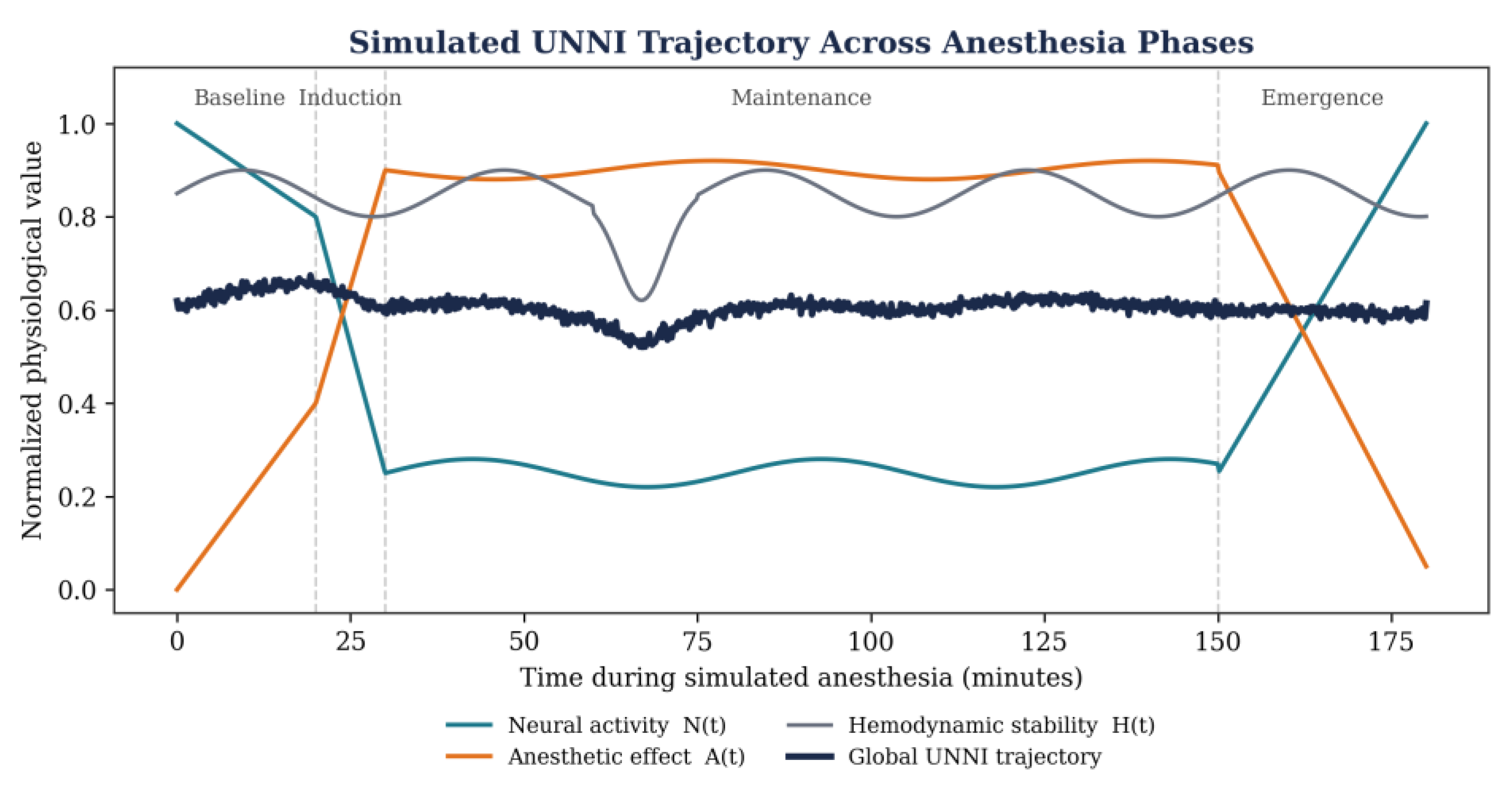
Simulated temporal evolution of neuronal activity, anesthetic concentration, and hemodynamic stability contributing to the global UNNI trajectory across baseline, induction, maintenance, and emergence phases.

Table 3. Mathematical variables and computational components of the UNNI framework.

Variable	Mathematical Representation	Biological Meaning
N(t)	Neural activity function	Electrical brain activity
A(t)	Drug-response function	Anesthetic influence
H(t)	Hemodynamic function	Cerebral perfusion stability
M(t)	Metabolic function	Energy consumption
C(t)	Connectivity function	Neural network organization
W	Interaction matrix	System relationships

Table 3. Mathematical variables and computational components of the UNNI framework.

Variable	Mathematical Representation	Biological Meaning
N(t)	Neural activity function	Electrical brain activity
A(t)	Drug-response function	Anesthetic influence
H(t)	Hemodynamic function	Cerebral perfusion stability
M(t)	Metabolic function	Energy consumption
C(t)	Connectivity function	Neural network organization
W	Interaction matrix	System relationships

1.3. Limitations of Current Neuroanesthesia Monitoring Approaches

Although current monitoring technologies have significantly improved anesthetic management, most available systems analyze individual physiological parameters independently. Examples include EEG-based monitoring of cortical activity, hemodynamic monitoring, oxygenation assessment, and intracranial pressure monitoring.

However, these approaches may not fully capture the emergent behavior of the entire neurophysiological system. A mathematical framework such as UNNI attempts to overcome this limitation by integrating multiple dimensions into a unified theoretical model. [1,2,3,4,5,6,7,8,9,10]

1.4. Theoretical Foundations of UNNI and Its Relationship With Artificial Intelligence

The development of the Unified Neuroanesthesia Neural Index (UNNI) is based on the concept that the anesthetized brain behaves as a complex adaptive system, characterized by nonlinear interactions, feedback mechanisms, information processing, and dynamic adaptation.

Artificial intelligence and mathematical neuroscience have demonstrated that biological systems can be represented through computational architectures capable of identifying hidden relationships between multiple variables. The UNNI framework proposes that neuroanesthetic stability may be approached as a prediction problem in which multiple physiological inputs are transformed into a dynamic representation of brain state. [19,20,21,22,23,24,25,26,27,28,29,51,52,53,54,55,56,57,58,59,60]

1.4.1. Neuroanesthesia as a Computational State-Space Model

A state-space model provides a mathematical description of systems evolving over time:

$$X_{t+1}=F\left(X_t,U_t\right)+{ϵ}_t,Y_t=G\left(X_t\right)+{\eta }_t$$

Equation (11) — state-space formulation of neuroanesthesia

Where X_t is the internal neurophysiological state at time t, U_t is the external anesthetic input, Y_t is the measurable physiological output, F is the state transition function, G is the observation function, and ε_t, η_t are biological noise components. The measured signals (EEG, blood pressure, oxygenation) are not the entire brain state — they are only external representations of an internal physiological condition.

1.4.2. Neural Network Representation of UNNI

Artificial neural networks provide a mathematical method for approximating complex nonlinear relationships. The basic neural computation is:

$$z_i=\sum _{j=1}{w}_{ij}{x}_j+b_i,y_i=\varphi \left(z_i\right)$$

Equation (12) — neuron activation and output

Where x_j are input physiological variables, w_ij are connection weights, b_i is a bias parameter, and φ is a nonlinear activation function. In the UNNI framework, the input layer may include EEG characteristics, anesthetic concentration, mean arterial pressure, cerebral oxygenation, and metabolic indicators; the hidden layers represent complex interactions between these variables; and the final output represents a theoretical neuroanesthetic stability estimation.

Mathematical Model 9 — Artificial Neural Network Formulation of UNNI

$$\mathrm{U}\mathrm{N}\mathrm{N}\mathrm{I}\left(t\right)=\varphi \left(W_2\varphi \left(W_{1}X\left(t\right)+b_1\right)+b_2\right)$$

Equation (13) — two-layer neural network formulation of UNNI

The first transformation W₁X(t)+b₁ combines physiological signals; the nonlinear function φ extracts hidden patterns; and the second transformation produces UNNI(t) as the final theoretical representation of neuroanesthetic stability.

1.4.3. Learning Dynamics and Model Optimization

For future validation, UNNI could theoretically be optimized using machine learning algorithms. The error function may be represented as:

$$L={\displaystyle \frac{1}{n}}\sum _{i=1}^n(y_i-{\widehat{y}}_i{)}^2$$

Equation (14) — mean-squared prediction error

Mathematical Model 10 — Gradient-Based Optimization

$$W_{new}=W_{old}-\alpha {\displaystyle \frac{\partial L}{\partial W}}$$

Equation (15) — gradient-based weight update

This equation describes how the theoretical model could improve its predictions by reducing mathematical error. Future research using clinical datasets could determine whether UNNI parameters correlate with depth of anesthesia, neurological recovery, postoperative cognitive outcomes, and cerebral stability. [61,62,63,64,65,66,67,68,69,70]

1.4.4. Feedback Control and Adaptive Neuroanesthesia

The brain during anesthesia is continuously influenced by feedback mechanisms. A simplified control model can be expressed as:

$$u\left(t\right)=K\left(r\left(t\right)-y\left(t\right)\right)$$

Equation (16) — closed-loop anesthetic adjustment

Where u(t) is the anesthetic adjustment, r(t) is the desired physiological target, y(t) is the measured physiological state, and K is a control coefficient. If the measured brain state differs from the desired state, the model could theoretically adjust anesthetic administration — a principle consistent with future developments in closed-loop anesthesia delivery, artificial intelligence-assisted anesthesia, and personalized medicine.

Figure 3. Artificial neural network architecture of the UNNI model.

Figure 3. Artificial neural network architecture of the UNNI model.

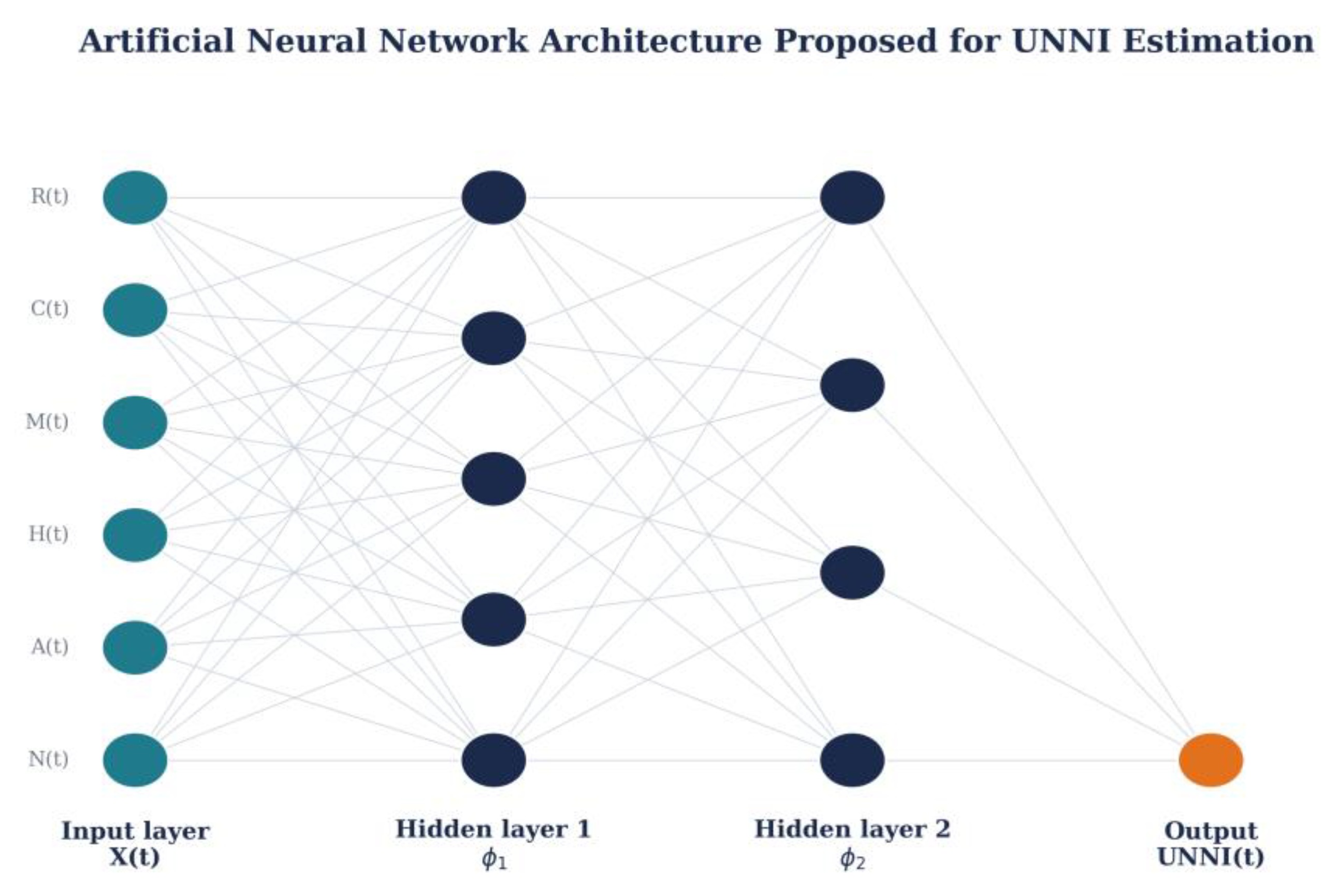
Physiological input variables, hidden computational layers, nonlinear transformations, and the final neuroanesthetic stability output.

Table 4. Artificial intelligence components incorporated into the theoretical UNNI framework.

AI Component	Mathematical Element	Neuroanesthesia Application
Input layer	X(t)	Physiological data acquisition
Hidden layers	W, φ	Pattern recognition
Output layer	UNNI(t)	Stability estimation
Loss function	L	Model evaluation
Optimization	Gradient descent	Parameter adjustment

Table 4. Artificial intelligence components incorporated into the theoretical UNNI framework.

AI Component	Mathematical Element	Neuroanesthesia Application
Input layer	X(t)	Physiological data acquisition
Hidden layers	W, φ	Pattern recognition
Output layer	UNNI(t)	Stability estimation
Loss function	L	Model evaluation
Optimization	Gradient descent	Parameter adjustment

1.5. Summary of Introduction

This first section establishes the theoretical foundation of UNNI by integrating mathematical modeling, differential calculus, algebraic representation, dynamic systems theory, and artificial neural networks. The proposed framework considers anesthesia not as a collection of independent physiological measurements, but as a continuously evolving mathematical system. The next section develops the central mathematical architecture of UNNI in full.

2. Mathematical Foundation of the Unified Neuroanesthesia Neural Index (UNNI)

2.1. Mathematical Representation of the Neuroanesthetic State Space

The human brain during anesthesia can be considered a high-dimensional dynamic system in which multiple physiological variables interact simultaneously. In classical mathematical modeling, complex systems are represented through a state-space approach, where the complete condition of the system is described by a vector containing all relevant variables. For the proposed UNNI framework, the neuroanesthetic state vector is extended to six dimensions:

$$X\left(t\right)={\left[,N,\left(t\right),,,A\left(t\right)H\left(t\right)M\left(t\right)C\left(t\right)R\left(t\right)\right]}^T\in \mathcal{l}{R}^6$$

Equation (17) — six-dimensional neuroanesthetic state vector

Where R(t) is the recovery and resilience factor, added to the five domains introduced in Section 1. This vector transforms neuroanesthesia from a single-variable observation into a multidimensional mathematical space: X(t) ∈ ℝ⁶ means that the neuroanesthetic state exists mathematically in a six-dimensional physiological domain.

2.2. Algebraic Construction of the UNNI Core Equation

The fundamental hypothesis of UNNI is that global neuroanesthetic stability emerges from weighted interactions between physiological domains:

$$\mathrm{U}\mathrm{N}\mathrm{N}\mathrm{I}\left(t\right)=\sum _{i=1}^6{w}_i{X}_i\left(t\right)+\sum _{i=1}^6\sum _{j=1}^6{\beta }_{ij}{X}_i\left(t\right)X_j\left(t\right)$$

Equation (18) — algebraic UNNI core equation with pairwise interactions

Where X_i(t) are individual physiological variables, w_i are linear contribution coefficients, and β_ij are nonlinear interaction coefficients. The first term represents direct physiological influence; the second term represents biological interactions — for example, neuronal activity and anesthetic concentration (N×A), cerebral metabolism and blood flow (M×H), and connectivity and recovery capacity (C×R). These interactions create nonlinear behavior.

2.3. Differential Calculus Model of UNNI Evolution

Because anesthesia is a time-dependent process, the mathematical model must include temporal variation:

$${\displaystyle \frac{d\left(\mathrm{U}\mathrm{N}\mathrm{N}\mathrm{I}\right)}{dt}}=F\left(X,\left(t\right),U\left(t\right)\theta \right)$$

Equation (19) — temporal evolution of UNNI

The derivative d(UNNI)/dt represents the velocity of change of neuroanesthetic stability. Three regimes are possible: a stable state where d(UNNI)/dt ≈ 0; progressive deterioration where d(UNNI)/dt < 0; and improvement where d(UNNI)/dt > 0.

2.4. Integral Model of Cumulative Neuroanesthetic Exposure

The effect of anesthesia depends not only on the current concentration but also on previous exposure. Cumulative anesthetic influence is modeled with an exponential decay kernel:

$$A_c\left(t\right)={\int }_0^{t}A\left(\tau \right)e^{-k\left(t-\tau \right)}d\tau$$

Equation (20) — cumulative anesthetic exposure with exponential decay

Where A_c(t) is the cumulative anesthetic effect, A(τ) is the anesthetic concentration history, and k is the elimination constant; the exponential term represents drug elimination and biological decay. Two patients receiving the same anesthetic dose may have different physiological responses because metabolism, receptor sensitivity, and cerebral reserve differ — the integral model attempts to mathematically represent this individual variability.

2.5. Matrix Formulation of UNNI Interactions

The relationships between the six physiological components can be represented as a 6×6 interaction matrix B:

$$Y\left(t\right)=BX\left(t\right),B=\left[\begin{array}{cccc}{b}_{11}& b_{12}& ...& b_{16}\\ b_{21}& b_{22}& ...& b_{26}\\ ⋮& ⋮& \ddots & ⋮\\ b_{61}& b_{62}& ...& b_{66}\end{array}\right]$$

Equation (21) — 6×6 interaction matrix formulation

Each element b_ij represents the influence of variable j on variable i — for example, b_NA represents the effect of anesthetic concentration on neuronal activity, and b_HM represents the relationship between hemodynamic status and metabolism.

Figure 4. Mathematical state-space representation of the UNNI framework.

Figure 4. Mathematical state-space representation of the UNNI framework.

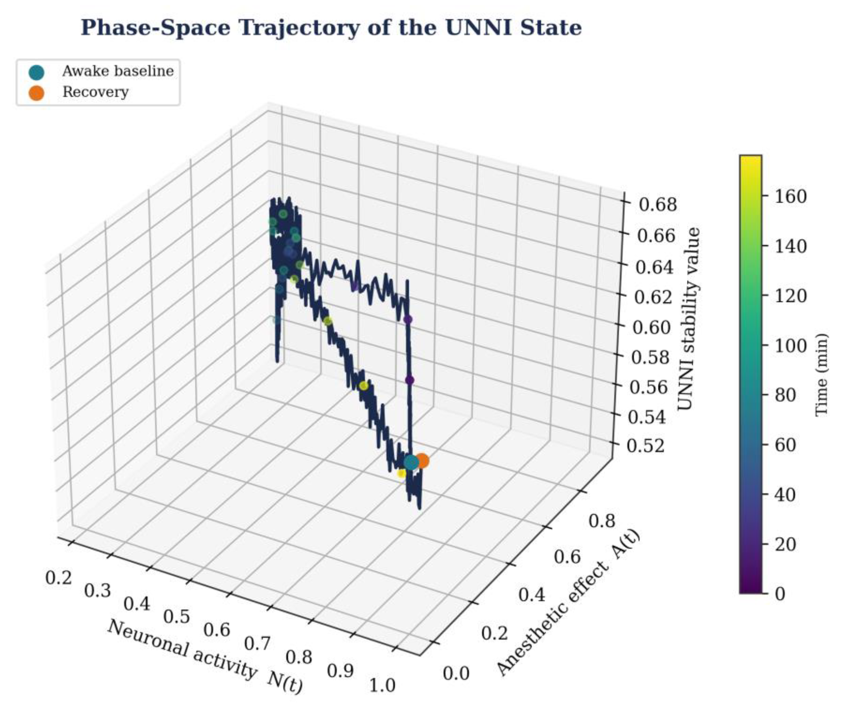
Simulated three-dimensional phase-space trajectory showing transitions between awake, anesthetized, and recovery states across neuronal activity, anesthetic effect, and UNNI stability axes.

Table 5. Mathematical structure of the UNNI framework.

Mathematical Element	Symbol	Function
State vector	X(t)	Represents physiological condition
Weight coefficients	w_i	Linear contribution
Interaction matrix	B	Biological relationships
Differential operator	d/dt	Temporal evolution
Integral operator	∫	Cumulative effects
Nonlinear function	F	Complex biological behavior

Table 5. Mathematical structure of the UNNI framework.

Mathematical Element	Symbol	Function
State vector	X(t)	Represents physiological condition
Weight coefficients	w_i	Linear contribution
Interaction matrix	B	Biological relationships
Differential operator	d/dt	Temporal evolution
Integral operator	∫	Cumulative effects
Nonlinear function	F	Complex biological behavior

2.6. Mathematical Stability Analysis of UNNI

2.6.1. Concept of Stability in Neuroanesthetic Systems

In mathematical systems theory, stability describes the ability of a dynamic system to maintain or return to an equilibrium state after a disturbance. During anesthesia, the brain is continuously exposed to internal and external perturbations, including variations in anesthetic concentration, changes in cerebral perfusion, metabolic fluctuations, surgical stimulation, and physiological stress responses. The UNNI framework therefore requires a mathematical stability component capable of describing whether the neuroanesthetic state remains controlled or moves toward instability. [30,31,32,33,34,35,36,37,38,39,40,41]

Mathematical Model 11 — Linearized UNNI Dynamic System

Near an equilibrium point X*, the UNNI system can be approximated as a linear time-invariant system:

$${\displaystyle \frac{dX}{dt}}=AX\left(t\right)+BU\left(t\right)$$

Equation (22) — linearized dynamic system near equilibrium

Where A is the system dynamics matrix, B is the input influence matrix, X(t) is the neurophysiological state vector, and U(t) is the anesthetic input vector. A stable brain state during anesthesia requires that disturbances decrease over time; the behavior of the system depends on the eigenvalues of matrix A.

2.6.2. Eigenvalue Analysis of Neuroanesthetic Stability

$$det\left(A-\lambda I\right)=0$$

Equation (23) — eigenvalue equation

If Re(λ) < 0 the system theoretically returns toward equilibrium; if Re(λ) > 0 the system may move away from equilibrium. A stable anesthetic state may correspond to controlled neuronal suppression, preserved cerebral perfusion, and balanced metabolism, whereas an unstable state may correspond to excessive neuronal depression, hemodynamic collapse, and impaired cerebral regulation.

Mathematical Model 12 — Lyapunov Stability Function

$$V\left(X\right)=X^{T}PX,{\displaystyle \frac{dV}{dt}}<0$$

Equation (24) — Lyapunov stability function and condition

Where P is a positive-definite matrix. The Lyapunov approach evaluates whether the energy of a mathematical system decreases with time; a decreasing function dV/dt < 0 indicates that the system is moving toward a stable physiological condition.

Mathematical Model 13 — Perturbation Response Function

$$\Delta X\left(t\right)=G\left(t\right)\Delta U\left(t\right)$$

Equation (25) — perturbation response to external stimulation

This equation represents how the brain responds to surgical stimulation, painful stimulation, blood pressure changes, or rapid anesthetic adjustment. A robust neuroanesthetic system should minimize excessive deviations.

Mathematical Model 14 — Resilience Factor in UNNI

$$R_f={\displaystyle \frac{\Delta X_{recovered}}{\Delta X_{initial}}}$$

Equation (26) — physiological resilience factor

A higher resilience factor R_f indicates faster physiological adaptation, better recovery capacity, and greater stability; a lower value may indicate vulnerability to disturbances.

2.7. Composite Stability Equation of UNNI

By integrating algebra, calculus, and stability theory, the global theoretical model becomes:

$$\mathrm{U}\mathrm{N}\mathrm{N}\mathrm{I}\left(t\right)=\sum w_i{X}_i\left(t\right)+\sum {\beta }_{ij}{X}_i\left(t\right)X_j\left(t\right)+\lambda {\int }_0^{t}F\left(X\left(\tau \right)\right)d\tau +\mu R_f$$

Equation (27) — composite UNNI stability equation

This equation combines four mathematical domains: (1) linear algebra, Σw_iX_i, representing individual physiological contributions; (2) nonlinear algebra, Σβ_ijX_iX_j, representing biological interactions; (3) integral calculus, λ∫F(X(τ))dτ, representing accumulated physiological history; and (4) stability theory, μR_f, representing recovery capacity.

Figure 5. Mathematical stability landscape of the UNNI framework.

Figure 5. Mathematical stability landscape of the UNNI framework.

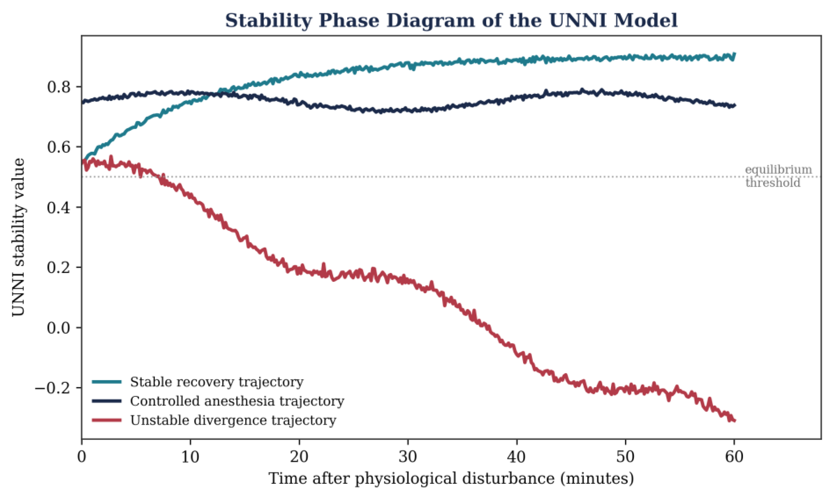
Simulated stability phase diagram showing stable recovery, controlled anesthesia, and unstable divergence trajectories relative to the theoretical equilibrium threshold.

Table 6. Mathematical stability parameters included in the UNNI framework.

Parameter	Mathematical Concept	Physiological Interpretation
Eigenvalues	Dynamic response	System stability
Lyapunov function	Energy-like stability measure	Return toward equilibrium
Perturbation function	External response	Surgical stimulation effect
Resilience factor	Recovery ratio	Adaptive capacity
Stability derivative	Temporal change	Direction of evolution

Table 6. Mathematical stability parameters included in the UNNI framework.

Parameter	Mathematical Concept	Physiological Interpretation
Eigenvalues	Dynamic response	System stability
Lyapunov function	Energy-like stability measure	Return toward equilibrium
Perturbation function	External response	Surgical stimulation effect
Resilience factor	Recovery ratio	Adaptive capacity
Stability derivative	Temporal change	Direction of evolution

2.8. Numerical Simulation Framework for UNNI

2.8.1. Purpose of Computational Simulation

Before clinical implementation, any theoretical mathematical model requires computational evaluation to examine its internal behavior. The proposed UNNI framework can be explored through numerical simulation to determine whether the mathematical structure produces biologically plausible patterns. The objective of simulation is not to prove clinical validity, but to evaluate mathematical consistency, system stability, sensitivity to parameter variation, and potential predictive behavior.

The simulation framework represents a hypothetical neuroanesthetic environment in which physiological variables change dynamically during induction, maintenance, and recovery phases of anesthesia.

2.8.2. Normalization of Physiological Variables

Because physiological parameters have different measurement units, normalization is required before mathematical integration:

$$Z_i\left(t\right)={\displaystyle \frac{X_i\left(t\right)-X_{min}}{X_{max}-X_{min}}}$$

Equation (28) — min–max normalization of physiological variables

This transformation converts different physiological measurements into a common mathematical scale, 0 ≤ Z_i(t) ≤ 1, allowing variables such as EEG activity, blood pressure, metabolic indicators, and anesthetic concentration to be combined within the same computational model.

2.8.3. Simulated UNNI State Equation

After normalization, the theoretical UNNI function can be expressed as:

$$\mathrm{U}\mathrm{N}\mathrm{N}\mathrm{I}\left(t\right)=\sum _{i=1}^6{w}_i{Z}_i\left(t\right)+\sum _{i,j=1}^6{\beta }_{ij}{Z}_i\left(t\right)Z_j\left(t\right)$$

Equation (29) — normalized simulated UNNI state equation

For computational demonstration only, the following hypothetical parameters were used to explore model behavior. These values are mathematical assumptions for model exploration and do not represent clinical thresholds.

Table 7. Hypothetical weighting parameters used for computational demonstration.

Variable	Symbol	Hypothetical Weight
Neural activity	N(t)	0.30
Anesthetic effect	A(t)	0.25
Hemodynamic stability	H(t)	0.20
Metabolic state	M(t)	0.15
Connectivity	C(t)	0.07
Recovery factor	R(t)	0.03

Table 7. Hypothetical weighting parameters used for computational demonstration.

Variable	Symbol	Hypothetical Weight
Neural activity	N(t)	0.30
Anesthetic effect	A(t)	0.25
Hemodynamic stability	H(t)	0.20
Metabolic state	M(t)	0.15
Connectivity	C(t)	0.07
Recovery factor	R(t)	0.03

2.8.4. Temporal Simulation Using Differential Equations

$${\mathrm{U}\mathrm{N}\mathrm{N}\mathrm{I}}_{t+1}={\mathrm{U}\mathrm{N}\mathrm{N}\mathrm{I}}_t+\Delta t{\displaystyle \frac{d\left(\mathrm{U}\mathrm{N}\mathrm{N}\mathrm{I}\right)}{dt}}$$

Equation (30) — recursive temporal simulation of UNNI

This equation allows the model to follow the trajectory of neuroanesthetic stability over time. During induction, A(t) ↑ may produce N(t) ↓; during recovery, A(t) ↓ may produce N(t) ↑. The final UNNI trajectory represents the combined response of all state variables (Figure 2).

2.8.5. Sensitivity Analysis of UNNI Parameters

A mathematical model must evaluate how sensitive the output is to changes in input variables:

$$S_i={\displaystyle \frac{\partial \mathrm{U}\mathrm{N}\mathrm{N}\mathrm{I}}{\partial X_i}}$$

Equation (31) — sensitivity coefficient of UNNI with respect to a parameter

The sensitivity coefficient describes how much UNNI changes when one physiological parameter changes. For example, S_A = ∂UNNI/∂A represents the theoretical influence of anesthetic concentration; a higher sensitivity indicates that small variations in the variable may strongly influence the overall model.

Figure 6. Simulated parameter sensitivity of the UNNI model.

Figure 6. Simulated parameter sensitivity of the UNNI model.

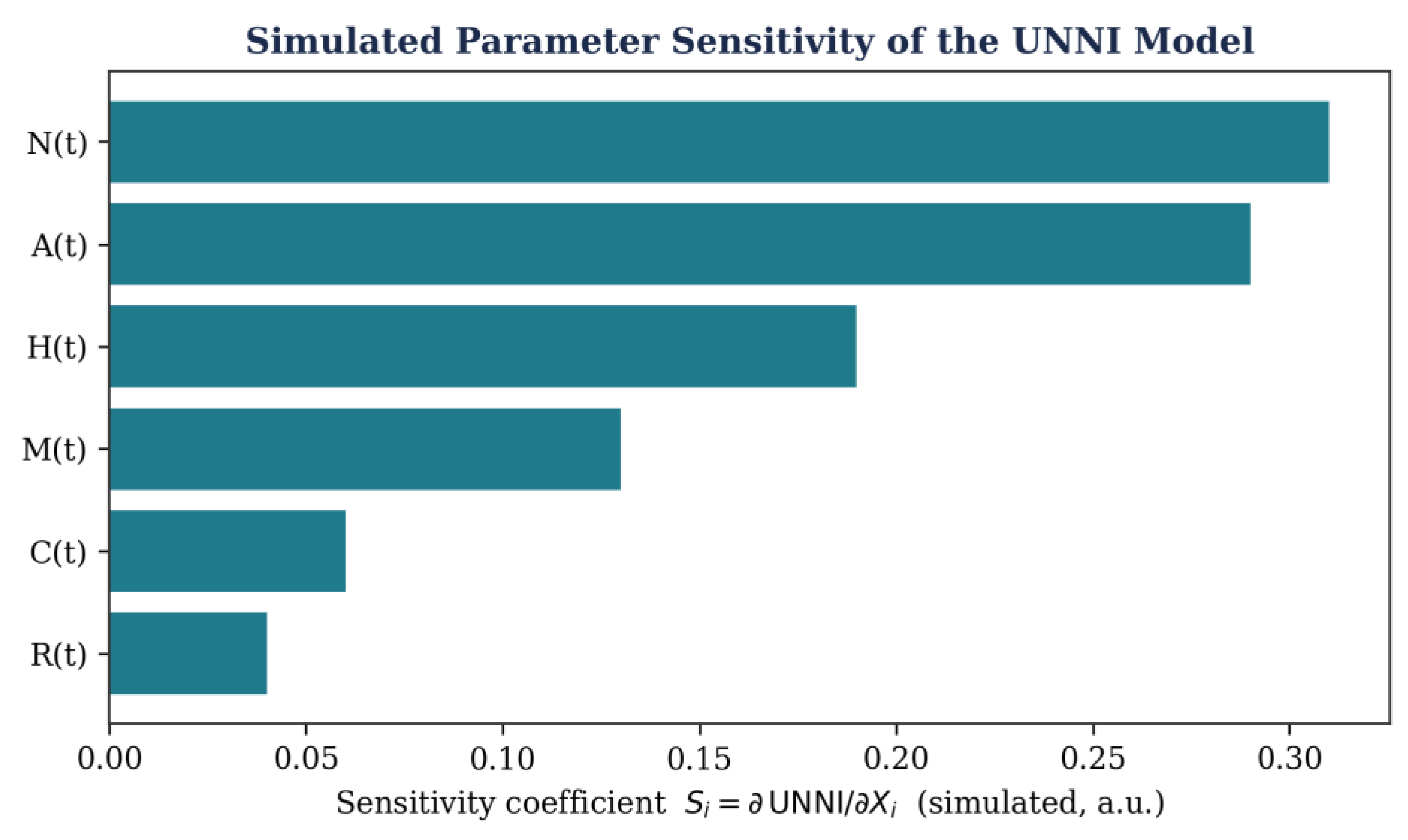
Hypothetical sensitivity coefficients (arbitrary units) illustrating the relative theoretical influence of each state-vector component on the composite UNNI output.

2.8.6. Computational Algorithm for UNNI Simulation

The proposed computational pipeline follows six sequential steps:

• Step 1: Acquire physiological variables, X(t) = [N, A, H, M, C, R].
• Step 2: Normalize all variables, X(t) → Z(t).
• Step 3: Apply the weighted mathematical transformation, WZ(t).
• Step 4: Calculate nonlinear interactions, β_ij Z_i Z_j.
• Step 5: Integrate temporal effects, ∫F(Z(t)) dt.
• Step 6: Generate the final UNNI trajectory.

Table 8. Proposed computational workflow for numerical simulation of UNNI.

Simulation Step	Mathematical Operation	Purpose
Data acquisition	X(t)	Collect physiological inputs
Normalization	Z_i(t)	Standardize variables
Weighting	w_i Z_i	Estimate contribution
Interaction analysis	β_ij Z_i Z_j	Model nonlinear effects
Integration	∫F(X) dt	Include time dependency
Output generation	UNNI(t)	Estimate theoretical stability

Table 8. Proposed computational workflow for numerical simulation of UNNI.

Simulation Step	Mathematical Operation	Purpose
Data acquisition	X(t)	Collect physiological inputs
Normalization	Z_i(t)	Standardize variables
Weighting	w_i Z_i	Estimate contribution
Interaction analysis	β_ij Z_i Z_j	Model nonlinear effects
Integration	∫F(X) dt	Include time dependency
Output generation	UNNI(t)	Estimate theoretical stability

2.9. Mathematical Limitations of the Proposed Model

Although UNNI provides an integrated theoretical structure, several limitations must be recognized:

• Biological systems contain unpredictable variability.
• Mathematical coefficients require empirical determination.
• Clinical validation requires large datasets.
• Neural responses cannot be completely represented by equations alone.
• Model predictions may differ between individuals.

UNNI should therefore currently be considered a conceptual computational framework requiring experimental and clinical validation.

3. Computational Neural Network Model of the Unified Neuroanesthesia Neural Index (UNNI)

3.1. Integration of Artificial Intelligence and Mathematical Neuroanesthesia Modeling

The increasing development of artificial intelligence (AI) and computational neuroscience provides new opportunities for analyzing complex biological systems. The human brain during anesthesia represents a nonlinear adaptive network where multiple physiological signals interact simultaneously. Traditional statistical approaches may not fully capture these complex relationships because the relationship between physiological inputs and neurological outcomes is often nonlinear.

Artificial neural networks (ANNs) provide a mathematical framework capable of approximating complex functions by learning relationships between multiple input variables. In the proposed UNNI framework, the neural network does not replace physiological interpretation; rather, it provides a computational layer capable of integrating multidimensional biological information. [51,52,53,54,55,56,57,58,59,60]

3.2. Architecture of the UNNI Artificial Neural Network

The proposed computational architecture consists of three principal components.

1. Input Layer

The input layer receives the normalized physiological parameters X(t) = [N(t), A(t), H(t), M(t), C(t), R(t)].

2. Hidden Computational Layers

The hidden layers perform mathematical transformations and identify complex relationships between variables, following the same general neuron-activation form introduced as Equation (12) in Section 1.4.2: h_k = φ(Σw_ki x_i + b_k), where h_k is the hidden neuron activation, w_ki is the connection weight, b_k is the bias parameter, and φ is a nonlinear activation function.

3. Output Layer

The final layer generates the theoretical UNNI value as a weighted, biased, and nonlinearly transformed combination of the hidden activations:

$$h_k=\varphi \left(\sum _{i=1}^n{w}_{ki}{x}_i+b_k\right),\mathrm{U}\mathrm{N}\mathrm{N}\mathrm{I}\left(t\right)=\varphi \left(\sum _{k=1}^m{v}_k{h}_k+c\right)!$$

Equation (32) — hidden-to-output transformation of the UNNI network

Where v_k are the output weights and c is the output bias.

Mathematical Model 15 — Multilayer Neural Representation

$$\mathrm{U}\mathrm{N}\mathrm{N}\mathrm{I}\left(t\right)={\varphi }_3\left(W_3{\varphi }_2\left(W_2{\varphi }_1\left(W_{1}X\left(t\right)+b_1\right)+b_2\right)+b_3\right)$$

Equation (33) — multilayer (deep) neural network formulation of UNNI

This equation represents a deep computational model. The first layer W₁X(t)+b₁ combines physiological inputs; the intermediate transformations φ₁, φ₂ extract hidden patterns; and the final transformation φ₃ produces the predicted neuroanesthetic stability index.

Figure 7. Artificial neural network architecture proposed for UNNI calculation.

Figure 7. Artificial neural network architecture proposed for UNNI calculation.

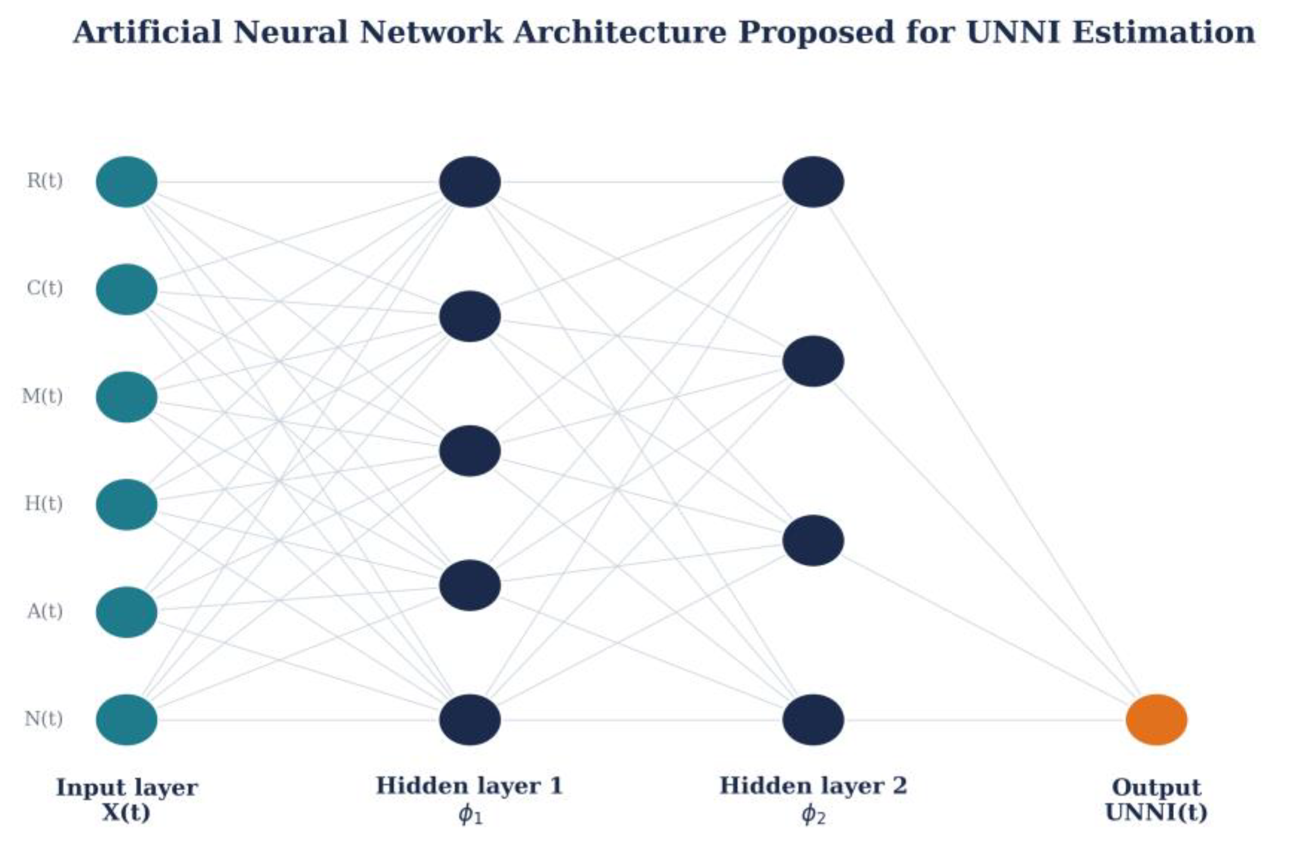
Physiological input variables, hidden computational layers, and final neuroanesthetic stability output of the multilayer UNNI network.

3.4. Activation Functions and Biological Nonlinearity

Biological systems rarely behave linearly; nonlinear activation functions are therefore required. One possible function is the sigmoid function:

$$\sigma \left(x\right)={\displaystyle \frac{1}{1+e^{-x}}}$$

Equation (34) — sigmoid activation function

The sigmoid function converts continuous mathematical values into bounded outputs 0 < σ(x) < 1, which may theoretically represent transitions between physiological states such as low neural stability, intermediate anesthetic state, and high recovery state.

Mathematical Model 16 — Rectified Linear Activation Function

$$\mathrm{R}\mathrm{e}\mathrm{L}\mathrm{U}\left(x\right)=max\left(0,x\right)$$

Equation (35) — ReLU activation function

This function allows the model to ignore insignificant negative signals while amplifying important positive changes — potentially representing threshold responses such as sudden EEG changes, rapid hemodynamic deterioration, or abrupt recovery transitions.

3.5. Learning Mechanism: Backpropagation Optimization

A neural network improves its parameters by minimizing prediction error:

$$L\left(\theta \right)={\displaystyle \frac{1}{n}}\sum _{i=1}^n{\left(Y_i-{\widehat{Y}}_i\right)}^2$$

Equation (36) — mean-squared loss function

Mathematical Model 17 — Weight Update Equation

$$W_{new}=W_{old}-\eta {\displaystyle \frac{\partial L}{\partial W}}$$

Equation (37) — gradient-descent weight update with learning rate η

During computational training the model generates a prediction, the error is calculated, the weights are adjusted, and the model gradually improves. This process allows future research to evaluate whether UNNI predictions correspond with clinical outcomes.

Figure 8. Simulated learning curve of the UNNI neural network.

Figure 8. Simulated learning curve of the UNNI neural network.

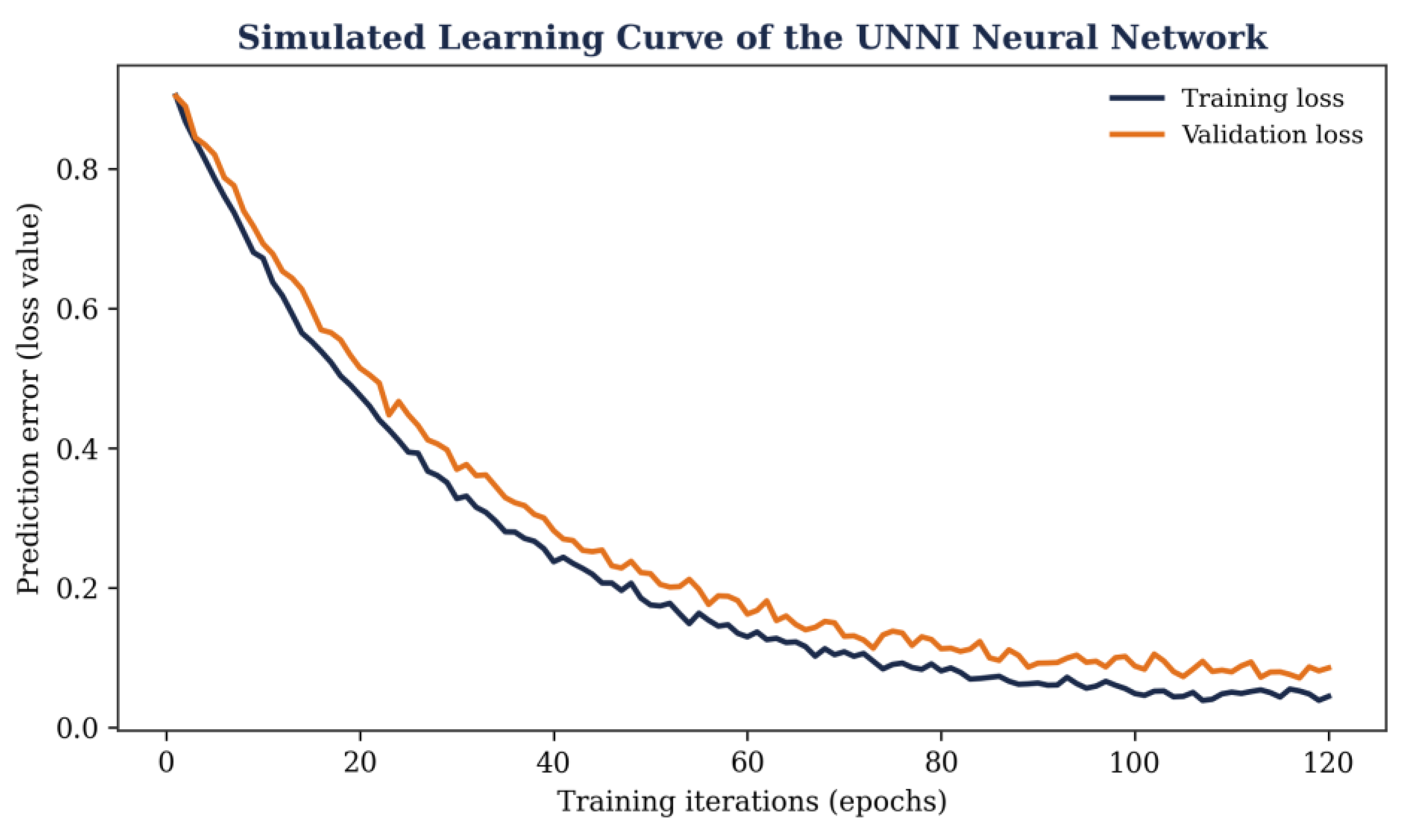
Hypothetical training and validation loss over 120 training iterations, illustrating the theoretical optimization process of UNNI prediction accuracy.

3.6. Recurrent Neural Network Model for Dynamic Anesthesia States

Because anesthesia is a continuous process, temporal information is essential. A recurrent neural network (RNN) can be represented as:

$$h_t=\varphi \left(W_x{X}_t+W_h{h}_{t-1}+b\right)$$

Equation (38) — recurrent hidden-state update

Where h_t is the current hidden state and h_{t-1} is the previous state memory. The previous condition of the brain influences the current state, reflecting anesthetic accumulation, delayed drug effects, and physiological adaptation.

Table 9. Neural network components of the proposed UNNI computational architecture.

Component	Mathematical Representation	Function
Input layer	X(t)	Physiological data
Hidden layer	h_k	Feature extraction
Activation function	φ(x)	Nonlinear transformation
Output layer	UNNI(t)	Stability estimation
Loss function	L	Error measurement
Optimization	Gradient descent	Model improvement

Table 9. Neural network components of the proposed UNNI computational architecture.

Component	Mathematical Representation	Function
Input layer	X(t)	Physiological data
Hidden layer	h_k	Feature extraction
Activation function	φ(x)	Nonlinear transformation
Output layer	UNNI(t)	Stability estimation
Loss function	L	Error measurement
Optimization	Gradient descent	Model improvement

3.7. Advanced Artificial Intelligence Extensions of the UNNI Framework

3.7.1. Long Short-Term Memory Networks for Neuroanesthetic Dynamics

Because anesthesia represents a continuous temporal process, the mathematical model must consider the influence of previous physiological states on the current brain condition. Standard artificial neural networks process information independently, while biological systems contain memory-dependent behavior. Advanced recurrent architectures such as Long Short-Term Memory (LSTM) networks — containing an input gate, forget gate, output gate, and memory cell — may provide a theoretical computational approach for modeling temporal neuroanesthetic evolution. [58,59,60]

Mathematical Model 18 — LSTM Memory Update Equation

$$C_t=f_t{C}_{t-1}+i_t{\tilde{C}}_t$$

Equation (39) — LSTM cell memory update

Where C_t is the current memory state, C_{t-1} is the previous memory state, f_t is the forget gate, i_t is the input gate, and C̃_t is the candidate memory information. In anesthesia, previous physiological conditions may influence current responses because of drug accumulation, receptor adaptation, metabolic changes, and delayed neurological recovery — so memory-based models may theoretically improve prediction of dynamic brain states.

3.7.2. Attention Mechanism for Identifying Critical Physiological Signals

Modern artificial intelligence models can identify which variables contribute most strongly to a prediction. The attention mechanism assigns different importance values to different physiological inputs:

$$\mathrm{A}\mathrm{t}\mathrm{t}\mathrm{e}\mathrm{n}\mathrm{t}\mathrm{i}\mathrm{o}\mathrm{n}\left(Q,K,V\right)=\mathrm{S}\mathrm{o}\mathrm{f}\mathrm{t}\mathrm{m}\mathrm{a}\mathrm{x}\left({\displaystyle \frac{Q{K}^T}{\sqrt{d_k}}}\right)V$$

Equation (40) — scaled dot-product attention mechanism

Where Q, K, V are the query, key, and value matrices and d_k is a dimensional scaling factor. The attention mechanism allows the UNNI model to theoretically determine whether specific variables have greater influence at different anesthesia stages — for example, A(t) may dominate during induction, H(t) may receive higher importance during cardiovascular instability, and C(t), R(t) may become more significant during emergence.

Figure 9. Simulated attention-weight distribution across physiological variables.

Figure 9. Simulated attention-weight distribution across physiological variables.

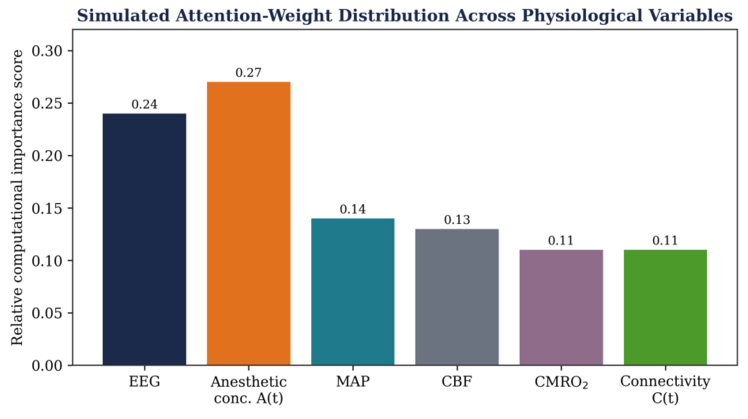
Hypothetical relative importance scores illustrating how an attention-based UNNI model may weight EEG, anesthetic concentration, MAP, CBF, CMRO2, and connectivity signals.

3.7.3. Transformer-Based UNNI Architecture

Transformer models have demonstrated strong performance in processing complex sequential information. A theoretical transformer-based UNNI model can be represented as:

$$Z=\mathrm{T}\mathrm{r}\mathrm{a}\mathrm{n}\mathrm{s}\mathrm{f}\mathrm{o}\mathrm{r}\mathrm{m}\mathrm{e}\mathrm{r}\left(X_1,X_2,.,..X_t\right)$$

Equation (41) — transformer-based sequence representation

Where X_t represents sequential physiological states and Z represents the learned neuroanesthetic representation. Instead of analyzing each physiological signal separately, the transformer architecture attempts to understand relationships across the entire temporal sequence, with potential applications including prediction of anesthetic depth, detection of neurological instability, and personalized anesthesia planning. [60]

Mathematical Model 19 — Integrated AI–UNNI Prediction Function

$${\widehat{Y}}_{UNNI}=F_{AI}\left({\mathrm{E}\mathrm{E}\mathrm{G},\mathrm{M}\mathrm{A}\mathrm{P},\mathrm{C}\mathrm{B}\mathrm{F},\mathrm{C}\mathrm{M}\mathrm{R}\mathrm{O}}_2,,A,\left(t\right)C\left(t\right)R\left(t\right)\right)$$

Equation (42) — integrated AI prediction function combining multimodal clinical signals

This equation represents a theoretical future model in which multiple clinical signals — EEG, mean arterial pressure, cerebral blood flow, and cerebral oxygen metabolic rate — are integrated into a single computational prediction. It does not imply immediate clinical use but provides a framework for future research.

3.7.4. Explainable Artificial Intelligence (XAI) in UNNI

A major limitation of artificial intelligence models is that complex algorithms may produce predictions without clear explanations. Explainable AI attempts to identify the contribution of each variable:

$${\mathrm{I}\mathrm{m}\mathrm{p}\mathrm{o}\mathrm{r}\mathrm{t}\mathrm{a}\mathrm{n}\mathrm{c}\mathrm{e}}_i={\displaystyle \frac{\Delta \mathrm{U}\mathrm{N}\mathrm{N}\mathrm{I}}{\Delta X_i}}$$

Equation (43) — feature-importance approximation for explainability

This mathematical relationship estimates how much the UNNI output changes when one physiological variable changes, improving transparency and potentially supporting clinical acceptance. [67,68,69,70]

Table 10. Advanced artificial intelligence approaches integrated into the theoretical UNNI framework.

AI Method	Mathematical Principle	Potential Application
LSTM	Temporal memory equations	Dynamic anesthesia prediction
Attention mechanism	Weighted information selection	Identification of critical variables
Transformer	Sequence modeling	Complex physiological integration
Explainable AI	Feature contribution analysis	Model transparency

Table 10. Advanced artificial intelligence approaches integrated into the theoretical UNNI framework.

AI Method	Mathematical Principle	Potential Application
LSTM	Temporal memory equations	Dynamic anesthesia prediction
Attention mechanism	Weighted information selection	Identification of critical variables
Transformer	Sequence modeling	Complex physiological integration
Explainable AI	Feature contribution analysis	Model transparency

3.8. Future Computational Validation Strategy

A theoretical UNNI model requires systematic validation before any clinical application. A possible validation pathway includes three phases.

Phase 1: Mathematical Validation

Objectives include verifying equation stability, analyzing parameter sensitivity, and testing computational behavior.

Phase 2: Simulation Validation

Using synthetic physiological datasets, computational brain models, and virtual anesthesia scenarios.

Phase 3: Clinical Validation

Potential future studies may evaluate correlations between UNNI predictions and EEG changes, anesthetic depth measurements, postoperative neurological outcomes, and recovery characteristics.

Table 11. Proposed validation stages of the Unified Neuroanesthesia Neural Index (UNNI).

Stage	Method	Objective
Mathematical	Equation analysis	Verify theoretical consistency
Computational	Simulation models	Evaluate dynamic behavior
Experimental	Physiological datasets	Test biological relevance
Clinical	Prospective studies	Assess clinical applicability

Table 11. Proposed validation stages of the Unified Neuroanesthesia Neural Index (UNNI).

Stage	Method	Objective
Mathematical	Equation analysis	Verify theoretical consistency
Computational	Simulation models	Evaluate dynamic behavior
Experimental	Physiological datasets	Test biological relevance
Clinical	Prospective studies	Assess clinical applicability

4. Clinical Interpretation, Applications, and Future Perspectives of the UNNI Framework

4.1. Translation of Mathematical Modeling Into Clinical Neuroanesthesia Concepts

The primary objective of the Unified Neuroanesthesia Neural Index (UNNI) is to establish a theoretical bridge between mathematical systems theory and clinical neuroanesthesia. Modern anesthesia management relies on continuous observation of multiple physiological parameters; however, interpretation of these parameters often remains fragmented because each measurement represents only one aspect of the overall cerebral state.

The UNNI framework proposes that the brain during anesthesia should be considered a dynamic biological network in which neuronal activity, anesthetic exposure, cerebral perfusion, metabolism, connectivity, and recovery capacity interact continuously. The mathematical model does not replace clinical judgment; instead, it provides a conceptual structure for integrating complex physiological information. [1,2,3,4,5,6,7,8,9,10,11,12,13,14,15,16,17,18]

4.2. Potential Clinical Domains of UNNI Application

4.2.1. Individualized Anesthetic Management

One potential future application of UNNI is personalized anesthesia. Currently, anesthetic dosing is influenced by patient age, weight, comorbidities, surgical requirements, and pharmacological characteristics. However, patients receiving identical doses may demonstrate different neurological responses. A mathematical model incorporating individual physiological characteristics may theoretically allow personalized estimation of anesthetic response. [71,72,73,74,75,76,77]

Mathematical Model 20 — Personalized Neuroanesthetic Response Function

$$\mathrm{R}\mathrm{e}\mathrm{s}\mathrm{p}\mathrm{o}\mathrm{n}\mathrm{s}\mathrm{e}\left(t\right)=F\left(\mathrm{P}\mathrm{a}\mathrm{t}\mathrm{i}\mathrm{e}\mathrm{n}\mathrm{t},\mathrm{D}\mathrm{r}\mathrm{u}\mathrm{g},\mathrm{P}\mathrm{h}\mathrm{y}\mathrm{s}\mathrm{i}\mathrm{o}\mathrm{l}\mathrm{o}\mathrm{g}\mathrm{y},\mathrm{T}\mathrm{i}\mathrm{m}\mathrm{e}\right)$$

Equation (44) — personalized response function

This equation represents the principle of precision anesthesia: different individuals may follow different mathematical trajectories under the same intervention.

4.2.2. Neurological Monitoring During Complex Neurosurgery

Neurosurgical procedures require exceptional control of cerebral physiology. Potential future UNNI applications may include theoretical integration of EEG monitoring, cerebral oxygenation, intracranial pressure, and cerebral blood flow, with the objective of creating a global representation of cerebral stability rather than isolated measurements. [11,12,13,14,15,16,17,18]

Mathematical Model 21 — Multimodal Cerebral Stability Function

$$CS\left(t\right)=f\left({\mathrm{E}\mathrm{E}\mathrm{G},\mathrm{C}\mathrm{B}\mathrm{F},\mathrm{I}\mathrm{C}\mathrm{P},\mathrm{C}\mathrm{M}\mathrm{R}\mathrm{O}}_2\right)$$

Equation (45) — multimodal cerebral stability function

4.2.3. Prediction of Recovery Dynamics

Post-anesthetic recovery represents another possible area of computational investigation. Recovery depends on drug elimination, neuronal restoration, metabolic recovery, and patient-specific factors. A theoretical recovery model can be expressed as:

$$R\left(t\right)=R_0{e}^{-kt}$$

Equation (46) — exponential recovery trajectory

Where R₀ is the initial recovery capacity and k is the recovery constant. The exponential model represents gradual physiological restoration after anesthetic exposure; however, real biological recovery is more complex and requires clinical validation.

4.3. Ethical and Scientific Considerations

Although artificial intelligence and mathematical modeling provide promising opportunities, several ethical principles must be considered.

1. Clinical Responsibility

Computational systems should support, not replace, anesthesiologists. The final clinical decision must remain under professional medical responsibility.

2. Data Quality and Bias

Artificial intelligence models depend on the quality of training data. Potential problems include incomplete datasets, population differences, and measurement errors. [78,79,80]

3. Transparency

Because medical decisions involve patient safety, computational models should provide interpretable outputs whenever possible.

Figure 10. Conceptual clinical integration pathway of the UNNI framework.

Figure 10. Conceptual clinical integration pathway of the UNNI framework.

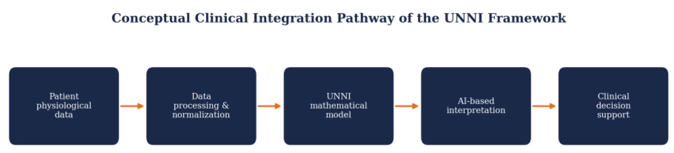
Proposed relationship between patient physiological data, data processing, the UNNI mathematical model, AI interpretation, and clinical decision support.

Table 12. Potential future clinical applications of the Unified Neuroanesthesia Neural Index (UNNI).

Clinical Domain	Current Approach	Possible UNNI Contribution
Anesthetic depth	Single-parameter monitoring	Integrated physiological model
Neurosurgery	Multimodal monitoring	Unified cerebral stability estimation
Recovery prediction	Clinical observation	Dynamic computational prediction
Personalized anesthesia	Population-based dosing	Individual physiological modeling

Table 12. Potential future clinical applications of the Unified Neuroanesthesia Neural Index (UNNI).

Clinical Domain	Current Approach	Possible UNNI Contribution
Anesthetic depth	Single-parameter monitoring	Integrated physiological model
Neurosurgery	Multimodal monitoring	Unified cerebral stability estimation
Recovery prediction	Clinical observation	Dynamic computational prediction
Personalized anesthesia	Population-based dosing	Individual physiological modeling

4.4. Limitations and Future Research Directions

The proposed UNNI framework remains a theoretical mathematical model, and several challenges must be addressed.

Mathematical Limitations

The current equations require empirical parameter estimation, validation of weighting coefficients, and testing of nonlinear assumptions.

Biological Limitations

The human brain contains complexity beyond mathematical representation. Important factors include genetic variability, psychological state, inflammatory responses, and unknown neural mechanisms.

Future Research Priorities

Future investigations should focus on the following priorities:

• Development of large neuroanesthesia datasets.
• Integration with EEG and imaging technologies.
• Artificial intelligence validation studies.
• Prospective clinical trials.
• Comparison with existing monitoring methods.

4.5. Final Theoretical Perspective

The Unified Neuroanesthesia Neural Index (UNNI) represents a conceptual attempt to describe anesthesia-induced brain changes using mathematical principles. By combining algebraic modeling, differential equations, integral calculus, dynamic systems theory, and artificial neural networks, UNNI provides a theoretical framework for future exploration of computational neuroanesthesia. The ultimate objective is not to simplify the human brain into a single equation, but to create mathematical tools capable of improving understanding of complex physiological interactions.

Physician by training, independent medical researcher, and author of medical and scientific publications, with a professional research focus on clinical neuroscience, neuroanesthesia, computational medicine, mathematical modeling, medical literature analysis, scientific writing, and medical education.

His research activities include the critical analysis and synthesis of medical literature, development of theoretical and computational frameworks for clinical research, mathematical modeling of physiological and neurological systems, preparation of scientific review and methodological manuscripts, development of evidence-informed medical educational content, and scientific communication and dissemination.

Article Type: Theoretical and Methodological Research Article

References are numbered sequentially in Vancouver style, grouped by thematic area for the reader’s convenience; in-text citation markers throughout the manuscript refer to this continuous numbering.

Neuroanesthesia, Anesthesia Physiology, and Brain Monitoring

Conclusion

Neuroanesthesia is fundamentally a dynamic interaction between pharmacology, physiology, and neural computation. The proposed UNNI model introduces a theoretical mathematical architecture in which neuroanesthetic stability emerges from multidimensional interactions over time.

Although extensive validation is required, this framework may provide a foundation for future research at the intersection of anesthesiology, neuroscience, mathematics, and artificial intelligence. Future studies should determine whether mathematical representations such as UNNI can contribute to safer, more personalized, and more predictive neuroanesthetic care.

References

- Mashour, G.A.; Avidan, M.S. Pharmacological and physiological mechanisms of consciousness during anesthesia. Anesthesiology 2018, 128(2), 311–324. [Google Scholar]
- Brown, E.N.; Purdon, P.L.; Van Dort, C.J. General anesthesia and altered states of brain network activity. Annu. Rev. Neurosci. 2011, 34, 601–628. [Google Scholar] [PubMed]
- Akeju, O.; Brown, E.N. Neural oscillations demonstrate that general anesthesia is a reversible coma. Anesth. Analg. 2017, 125(6), 2073–2085. [Google Scholar]
- Purdon, P.L.; Sampson, A.; Pavone, K.J.; Brown, E.N. Clinical electroencephalography for anesthesiologists: Part I. Background and basic signatures. Anesthesiology 2015, 123(4), 937–960. [Google Scholar] [CrossRef]
- Purdon, P.L.; Pierce, E.T.; Mukamel, E.A.; et al. Electroencephalogram signatures of loss and recovery of consciousness from propofol. Proc. Natl. Acad. Sci. 2013, 110(12), E1142–E1151. [Google Scholar] [CrossRef] [PubMed]
- Avidan, M.S.; Jacobsohn, E.; Glick, D.; et al. Prevention of intraoperative awareness in a high-risk surgical population. N. Engl. J. Med. 2011, 365, 591–600. [Google Scholar] [CrossRef] [PubMed]
- Leslie, K.; Davidson, A.J. Awareness during anesthesia. Anesthesiology 2010, 112(2), 256–267. [Google Scholar]
- Bonhomme, V.; Staquet, C.; Montupil, J.; et al. General anesthesia: an EEG-based approach to monitoring brain state. Curr. Opin. Anaesthesiol. 2019, 32(5), 613–620. [Google Scholar]
- Brown, E.N.; Lydic, R.; Schiff, N.D. General anesthesia, sleep, and coma. N. Engl. J. Med. 2010, 363, 2638–2650. [Google Scholar] [CrossRef] [PubMed]
- Hudetz, A.G. General anesthesia and the human brain: mechanisms of altered states of consciousness. Clin. Pharmacol. Ther. 2012, 91(2), 207–217. [Google Scholar]
- Cottrell, J.E.; Patel, P. Cottrell and Patel’s Neuroanesthesia, 6th ed.; Elsevier: Philadelphia, 2017. [Google Scholar]
- Miller, R.D.; Cohen, N.H.; Eriksson, L.I.; et al. Miller’s Anesthesia, 9th ed.; Elsevier: Philadelphia, 2020. [Google Scholar]
- Barash, P.G.; Cullen, B.F.; Stoelting, R.K.; et al. Clinical Anesthesia, 9th ed.; Wolters Kluwer: Philadelphia, 2023. [Google Scholar]
- Mutch, W.A.; El-Gabalawy, R.; Girling, L.; et al. Cerebral physiology during anesthesia. Can. J. Anesth. 2016, 63, 1050–1065. [Google Scholar]
- Citerio, G.; Cormio, M. Sedation in neurocritical care. Curr. Opin. Crit. Care 2003, 9(2), 90–97. [Google Scholar] [CrossRef] [PubMed]
- Drummond, J.C. Monitoring depth of anesthesia: clinical perspectives. Anesthesiol. Clin. 2016, 34(3), 539–551. [Google Scholar]
- Smith, M. Monitoring intracranial pressure and cerebral perfusion in neuroanesthesia. Br. J. Anaesth. 2017, 118(4), 491–502. [Google Scholar]
- Oddo, M.; Taccone, F.S.; et al. Brain oxygen monitoring in critically ill patients. Intensive Care Med. 2018, 44, 1609–1621. [Google Scholar]
- Tononi, G. Integrated information theory of consciousness: an updated account. Arch. Ital. De Biol. 2012, 150, 290–326. [Google Scholar]
- Dehaene, S.; Changeux, J.P. Experimental and theoretical approaches to conscious processing. Neuron 2011, 70(2), 200–227. [Google Scholar] [CrossRef] [PubMed]
- Mashour, G.A. Cognitive unbinding: a neuroscientific paradigm of general anesthesia and related states. Neurosci. Conscious. 2015, 2015(1), niv016. [Google Scholar]
- Friston, K.J. The free-energy principle: a unified brain theory? Nat. Rev. Neurosci. 2010, 11, 127–138. [Google Scholar] [CrossRef] [PubMed]
- Deco, G.; Jirsa, V.K.; McIntosh, A.R. Emerging concepts for the dynamical organization of resting-state activity. Nat. Rev. Neurosci. 2011, 12, 43–56. [Google Scholar] [CrossRef] [PubMed]
- Bassett, D.S.; Sporns, O. Network neuroscience. Nat. Neurosci. 2017, 20, 353–364. [Google Scholar] [CrossRef] [PubMed]
- Bullmore, E.; Sporns, O. Complex brain networks: graph theoretical analysis of structural and functional systems. Nat. Rev. Neurosci. 2009, 10, 186–198. [Google Scholar] [CrossRef] [PubMed]
- Sporns, O. Networks of the Brain; MIT Press: Cambridge, 2011. [Google Scholar]
- Breakspear, M. Dynamic models of large-scale brain activity. Nat. Neurosci. 2017, 20, 340–352. [Google Scholar] [CrossRef] [PubMed]
- Rabinovich, M.I.; Simmons, A.N.; Varona, P. Dynamical principles in neuroscience. Rev. Mod. Phys. 2012, 84, 101–128. [Google Scholar]
- Strogatz, S.H. Nonlinear Dynamics and Chaos: With Applications to Physics, Biology, Chemistry, and Engineering, 2nd ed.; Westview Press: Boulder, 2015. [Google Scholar]
- Hirsch, M.W.; Smale, S.; Devaney, R.L. Differential Equations, Dynamical Systems, and an Introduction to Chaos, 3rd ed.; Academic Press: Oxford, 2013. [Google Scholar]
- Perko, L. Differential Equations and Dynamical Systems, 3rd ed.; Springer: New York, 2001. [Google Scholar]
- Khalil, H.K. Nonlinear Systems, 3rd ed.; Prentice Hall: Upper Saddle River, 2002. [Google Scholar]
- Slotine, J.J.; Li, W. Applied Nonlinear Control; Prentice Hall: New Jersey, 1991. [Google Scholar]
- Sastry, S. Nonlinear Systems: Analysis, Stability, and Control; Springer: New York, 1999. [Google Scholar]
- Ljung, L. System identification: theory for the user, 2nd ed.; Prentice Hall: Upper Saddle River, 1999. [Google Scholar]
- Kalman, R.E. A new approach to linear filtering and prediction problems. J. Basic Eng. 1960, 82(1), 35–45. [Google Scholar] [CrossRef]
- Wiener, N. Cybernetics: Or Control and Communication in the Animal and the Machine; MIT Press: Cambridge, 1948. [Google Scholar]
- Bertalanffy, L.V. General system theory: foundations, development, applications; George Braziller: New York, 1968. [Google Scholar]
- Klir, G.J. Architecture of Systems Problem Solving; Springer: New York, 1985. [Google Scholar]
- Meiss, J.D. Differential Dynamical Systems; SIAM: Philadelphia, 2007. [Google Scholar]
- Dayan, P.; Abbott, L.F. Theoretical Neuroscience: Computational and Mathematical Modeling of Neural Systems; MIT Press: Cambridge, 2001. [Google Scholar]
- Izhikevich, E.M. Dynamical Systems in Neuroscience: The Geometry of Excitability and Bursting; MIT Press: Cambridge, 2007. [Google Scholar]
- Ermentrout, G.B.; Terman, D.H. Mathematical Foundations of Neuroscience; Springer: New York, 2010. [Google Scholar]
- Gerstner, W.; Kistler, W.M.; Naud, R.; Paninski, L. Neuronal Dynamics: From Single Neurons to Networks and Models of Cognition; Cambridge University Press: Cambridge, 2012. [Google Scholar]
- Koch, C. Biophysics of Computation: Information Processing in Single Neurons; Oxford University Press: Oxford, 2004. [Google Scholar]
- Wilson, H.R.; Cowan, J.D. Excitatory and inhibitory interactions in localized populations of model neurons. Biophys. Journal. 1972, 12(1), 1–24. [Google Scholar] [CrossRef] [PubMed]
- Hodgkin, A.L.; Huxley, A.F. A quantitative description of membrane current and its application to conduction and excitation in nerve. J. Physiol. 1952, 117, 500–544. [Google Scholar] [CrossRef] [PubMed]
- FitzHugh, R. Impulses and physiological states in theoretical models of nerve membrane. Biophys. J. 1961, 1, 445–466. [Google Scholar] [CrossRef] [PubMed]
- Morris, C.; Lecar, H. Voltage oscillations in the barnacle giant muscle fiber. Biophys. Journal. 1981, 35, 193–213. [Google Scholar] [CrossRef] [PubMed]
- Freeman, W.J. Mass Action in the Nervous System; Academic Press: New York, 1975. [Google Scholar]
- McCulloch, W.S.; Pitts, W. A logical calculus of the ideas immanent in nervous activity. Bull. Math. Biophys. 1943, 5, 115–133. [Google Scholar] [CrossRef]
- Rosenblatt, F. The perceptron: a probabilistic model for information storage and organization in the brain. Psychol. Rev. 1958, 65, 386–408. [Google Scholar] [CrossRef] [PubMed]
- Rumelhart, D.E.; Hinton, G.E.; Williams, R.J. Learning representations by back-propagating errors. Nature 1986, 323, 533–536. [Google Scholar] [CrossRef]
- LeCun, Y.; Bengio, Y.; Hinton, G.E. Deep learning. Nature 2015, 521, 436–444. [Google Scholar] [CrossRef] [PubMed]
- Goodfellow, I.; Bengio, Y.; Courville, A. Deep Learning; MIT Press: Cambridge, 2016. [Google Scholar]
- Bishop, C.M. Pattern Recognition and Machine Learning; Springer: New York, 2006. [Google Scholar]
- Hastie, T.; Tibshirani, R.; Friedman, J. The Elements of Statistical Learning, 2nd ed.; Springer: New York, 2009. [Google Scholar]
- Schmidhuber, J. Deep learning in neural networks: an overview. Neural Netw. 2015, 61, 85–117. [Google Scholar] [CrossRef] [PubMed]
- Hochreiter, S.; Schmidhuber, J. Long short-term memory. Neural Comput. 1997, 9(8), 1735–1780. [Google Scholar] [CrossRef] [PubMed]
- Vaswani, A.; Shazeer, N.; Parmar, N.; et al. Attention is all you need. Adv. Neural Inf. Process. Syst. 2017, 30, 5998–6008. [Google Scholar]
- Topol, E.J. High-performance medicine: the convergence of human and artificial intelligence. Nat. Med. 2019, 25, 44–56. [Google Scholar] [CrossRef] [PubMed]
- Rajkomar, A.; Dean, J.; Kohane, I. Machine learning in medicine. N. Engl. J. Med. 2019, 380, 1347–1358. [Google Scholar] [CrossRef] [PubMed]
- Esteva, A.; Robicquet, A.; Ramsundar, B.; et al. A guide to deep learning in healthcare. Nat. Med. 2019, 25, 24–29. [Google Scholar] [CrossRef] [PubMed]
- Yu, K.H.; Beam, A.L.; Kohane, I.S. Artificial intelligence in healthcare. Nat. Biomed. Eng. 2018, 2, 719–731. [Google Scholar] [CrossRef] [PubMed]
- Obermeyer, Z.; Emanuel, E.J. Predicting the future: big data, machine learning, and clinical medicine. N. Engl. J. Med. 2016, 375, 1216–1219. [Google Scholar] [CrossRef] [PubMed]
- Beam, A.L.; Kohane, I.S. Big data and machine learning in health care. JAMA 2018, 319(13), 1317–1318. [Google Scholar] [CrossRef] [PubMed]
- Chen, J.H.; Asch, S.M. Machine learning and prediction in medicine. N. Engl. J. Med. 2017, 376, 2507–2509. [Google Scholar] [CrossRef] [PubMed]
- Ghassemi, M.; Oakden-Rayner, L.; Beam, A.L. The false hope of current approaches to explainable artificial intelligence in health care. Lancet Digit. Health 2021, 3, e745–e750. [Google Scholar] [CrossRef] [PubMed]
- Holzinger, A.; Langs, G.; Denk, H.; Zatloukal, K.; Müller, H. Causability and explainability of artificial intelligence in medicine. WIREs Data Min. Knowl. Discov. 2019, 9, e1312. [Google Scholar] [CrossRef] [PubMed]
- Samek, W.; Wiegand, T.; Müller, K.R. Explainable artificial intelligence: understanding, visualizing and interpreting deep learning models. IT—Information Technol. 2017, 59, 243–249. [Google Scholar]
- Shafer, S.L.; Stanski, D.R. Improving the clinical utility of anesthetic pharmacology through pharmacokinetic and pharmacodynamic modeling. Anesthesiology 1992, 77, 665–673. [Google Scholar]
- Schnider, T.W.; Minto, C.F.; Gambus, P.L.; et al. The influence of method of administration and covariates on pharmacokinetics of propofol. Anesthesiology 1998, 88, 1170–1182. [Google Scholar] [CrossRef] [PubMed]
- Minto, C.F.; Schnider, T.W.; Shafer, S.L. Pharmacokinetics and pharmacodynamics of remifentanil. Anesthesiology 1997, 86, 10–23. [Google Scholar] [CrossRef] [PubMed]
- Eleveld, D.J.; Proost, J.H.; Vereecke, H.; Struys, M.M.R.F. An allometric model of propofol pharmacokinetics. Anesthesiology 2014, 120, 1041–1055. [Google Scholar] [CrossRef] [PubMed]
- Bouillon, T.W. Hypnotic and opioid anesthetic drug interactions. Anesthesiol. Clin. 2005, 23, 47–63. [Google Scholar]
- Stanski, D.R. Pharmacodynamic modeling in anesthesia. Anesthesiology 1992, 77, 1–5. [Google Scholar] [CrossRef] [PubMed]
- Shafer, S.L.; Gregg, K.M. Algorithms to rapidly achieve and maintain stable drug concentrations at the site of drug effect. J. Pharmacokinet. Pharmacodyn. 1992, 20, 147–169. [Google Scholar] [CrossRef] [PubMed]
- Ching, S.; Purdon, P.L.; Vijayan, S.; et al. A neurophysiological-metabolic model for burst suppression during anesthesia. PLoS Comput. Biol. 2012, 8, e1002465. [Google Scholar]
- Pritchett, K.; Shapcott, D.; et al. Quantitative EEG analysis during general anesthesia. Br. J. Anaesth. 2018, 121, 292–303. [Google Scholar]
- Kelz, M.B.; Mashour, G.A. The biology of general anesthesia from the perspective of sleep. Anesthesiology 2019, 130, 463–472. [Google Scholar]
- Lewis, L.D.; Weiner, V.S.; Mukamel, E.A.; et al. Rapid fragmentation of neuronal networks at the onset of propofol-induced unconsciousness. Neuron 2012, 74, 993–1002. [Google Scholar]
- Sarasso, S.; Boly, M.; Napolitani, M.; et al. Consciousness and complexity during general anesthesia. Sci. Transl. Med. 2015, 7, 306ra149. [Google Scholar]
- Casali, A.G.; Gosseries, O.; Rosanova, M.; et al. A theoretically based index of consciousness independent of sensory processing. Sci. Transl. Med. 2013, 5, 198ra105. [Google Scholar] [CrossRef] [PubMed]
- Alkire, M.T.; Hudetz, A.G.; Tononi, G. Consciousness and anesthesia. Science 2008, 322, 876–880. [Google Scholar] [CrossRef] [PubMed]
- Tononi, G.; Boly, M.; Massimini, M.; Koch, C. Integrated information theory: from consciousness to its physical substrate. Nat. Rev. Neurosci. 2016, 17, 450–461. [Google Scholar] [CrossRef] [PubMed]
- Johnson, K.W.; Torres Soto, J.; Glicksberg, B.S.; et al. Artificial intelligence in cardiology and medicine. J. Am. Coll. Cardiol. 2018, 71, 2668–2679. [Google Scholar] [CrossRef] [PubMed]
- Obermeyer, Z.; Powers, B.; Vogeli, C.; Mullainathan, S. Dissecting racial bias in an algorithm used to manage the health of populations. Science 2019, 366, 447–453. [Google Scholar] [CrossRef] [PubMed]
- Miotto, R.; Wang, F.; Wang, S.; Jiang, X.; Dudley, J.T. Deep learning for healthcare: review, opportunities and challenges. Brief. Bioinform. 2018, 19, 1236–1246. [Google Scholar] [CrossRef] [PubMed]
- Esteva, A.; Kuprel, B.; Novoa, R.A.; et al. Dermatologist-level classification of skin cancer with deep neural networks. Nature 2017, 542, 115–118. [Google Scholar] [CrossRef] [PubMed]
- Litjens, G.; Kooi, T.; Bejnordi, B.E.; et al. A survey on deep learning in medical image analysis. Med. Image Anal. 2017, 42, 60–88. [Google Scholar] [CrossRef] [PubMed]
Disclaimer/Publisher’s Note: The statements, opinions and data contained in all publications are solely those of the individual author(s) and contributor(s) and not of MDPI and/or the editor(s). MDPI and/or the editor(s) disclaim responsibility for any injury to people or property resulting from any ideas, methods, instructions or products referred to in the content. |
© 2026 by the authors. Licensee MDPI, Basel, Switzerland. This article is an open access article distributed under the terms and conditions of the Creative Commons Attribution (CC BY) license (http://creativecommons.org/licenses/by/4.0/).
Copyright: This open access article is published under a Creative Commons CC BY 4.0 license, which permit the free download, distribution, and reuse, provided that the author and preprint are cited in any reuse.