

Submitted:
13 August 2026
Posted:
17 August 2026
You are already at the latest version
Abstract
Classical turbulence closures systematically fail in high-Mach rotating flows because they introduce excessive dissipation and cannot capture the non-equilibrium effects that govern the dynamics. This limitation severely compromises the predictive reliability of thermal-hydraulic simulations for gas-cooled nuclear reactors. To overcome this challenge, we develop a rigorous numerical framework that seamlessly integrates a structure-preserving Lattice Boltzmann Method with a Physics-Informed Neural Network correction, grounded in hypocoercive stability theory. At the heart of our approach lies the Santos-Andrade inequality, a novel stability criterion that explicitly quantifies the competing influences of rotation, compressibility, and neural-network corrections, thereby offering a mathematically certified threshold for stable data-driven closures. We derive second-order convergence estimates for the semi-discrete LBM–PINN scheme and validate the framework against the canonical Taylor-Couette flow at Mach numbers 5.0 and 10.0. At Ma=10.0, classical closures — Smagorinsky, RANS, and SAS — fail catastrophically, producing unphysical constant temperature and pressure fields. In striking contrast, the Smagorinsky+PINN scheme uniquely restores a realistic radial temperature gradient and delivers a physically plausible Nusselt number of 17.14. The observed Lipschitz constant Lθ≈2.96 lies comfortably below the stability limit, confirming the practical utility of the Santos-Andrade criterion for high-fidelity nuclear thermal-hydraulic simulations.
Keywords:
high-Mach rotating turbulent flows
; Lattice Boltzmann method
; compressible turbulence
; physics-informed neural network
; Santos-Andrade hypocoercive inequality
MSC: 35Q35; 76F02; 76F55; 82C40; 68T07
1. Introduction
The modelling of high-speed rotating turbulent flows remains one of the most formidable challenges in computational fluid dynamics, with applications spanning from the intricate combustion dynamics inside gas turbine engines to the colossal accretion disks that power active galactic nuclei. The fundamental difficulty lies in the intricate, multi-scale interplay between compressibility, rotation, turbulence, and heat transfer — a combination that systematically frustrates classical modelling approaches. This introduction provides a concise survey of the evolution of turbulence modelling, tracing the intellectual lineage from early phenomenological closures through the rigorous mathematical foundations of kinetic theory and hypocoercivity, to the recent emergence of data-driven paradigms. We identify the critical gaps that motivate the present work and establish the scientific context for our contributions.
1.1. Historical Development of Turbulence Modelling
The modern era of turbulence modelling began with the systematic development of second-moment closures, epitomised by the Reynolds-stress transport equations introduced by Launder, Reece, and Rodi [7]. These formulations represented a significant advance over the simpler eddy-viscosity hypothesis, capturing the anisotropic nature of turbulent stresses in non-equilibrium flows. However, the closure still required empirical modelling of the pressure-strain and dissipation terms, introducing coefficients calibrated against canonical flows — a limitation that persisted across subsequent generations of models. These formulations were swiftly extended to capture the complex dynamics of astrophysical accretion disks by Begelman, Blandford, and Rees [11], while parallel experimental campaigns by Andereck, Liu, and Swinney [12] mapped the rich phenomenology of rotating instabilities in Taylor–Couette systems, establishing benchmark configurations for testing closure models.
Beyond these canonical astrophysical and aerospace applications, high-Mach rotating turbulent flows are of direct relevance to nuclear engineering, particularly in the thermal-hydraulic analysis of advanced reactor systems. In gas-cooled reactors (e.g., high-temperature gas-cooled reactors, HTGRs) and high-speed helium circulators, the clearance gaps between rotor and stator in canned motor pumps give rise to Taylor–Couette-like flows under extreme rotational speeds and significant temperature gradients [35,59]. The predictive accuracy of turbulence closures in such narrow, rotating annular passages directly impacts the assessment of coolant temperature distributions, flow resistance, and ultimately the safety margins of the reactor core. Classical eddy-viscosity models, calibrated for incompressible flows, are known to struggle in these regimes, motivating the development of structure-preserving, data-augmented closures with rigorous stability guarantees — a gap that the present work directly addresses.
The high computational cost of Reynolds-stress transport models gave rise to more accessible two-equation frameworks, most notably the k- model systematised by Wilcox [20]. While enormously successful in industrial practice, its reliance on the isotropic eddy-viscosity hypothesis fundamentally limits its ability to capture anisotropic turbulence in rotating flows, curved geometries, or regions of strong mean strain. Concurrently, the theoretical underpinnings of fluid behaviour were being rigorously re-examined through kinetic theory. Boltzmann’s equation [5] elegantly captures non-equilibrium phenomena beyond Newtonian constitutive relations, while Grad [2] provided a systematic method for deriving macroscopic equations through moment expansions. The Bhatnagar–Gross–Krook (BGK) approximation [1] dramatically simplified the kinetic equation while rigorously preserving conservation laws and the H-theorem. Lundgren [3] extended kinetic ideas to turbulence by deriving statistical distribution function equations, laying the groundwork for PDF-based modelling. The comprehensive treatises by Chapman and Cowling [13] and Glassey [18] established the rigorous mathematical foundations of the Boltzmann equation, inspiring later developments in hypocoercivity. Sarkar et al. [14] and Lele [17] systematically characterised compressibility effects on turbulence, identifying the key mechanisms that any credible compressible turbulence model must capture. Bertin’s comprehensive treatment of hypersonic aerothermodynamics [16] further underscored the importance of capturing high-Mach effects for aerospace and reactor applications.
The late 1990s witnessed two transformative developments. First, the Lattice Boltzmann Method (LBM), pioneered by Chen and Doolen [19], emerged as a numerical framework that explicitly solves a discretised kinetic equation, eliminating the need for an explicit pressure Poisson equation and offering exceptional parallelism. Second, Spalart and Allmaras [15] introduced a one-equation turbulence model tailored for aerodynamic applications. Succi’s comprehensive monograph [25] cemented LBM as a versatile computational technique. However, standard LBM formulations could violate the discrete H-theorem, leading to numerical instabilities at high Reynolds numbers. Boghosian et al. [22] addressed this by introducing entropic LBM formulations that rigorously enforce the H-theorem at the discrete level. Pope’s landmark textbook [24] synthesised the state of the art in turbulence modelling, while Heinz [26] bridged kinetic descriptions and engineering turbulence modelling by deriving a thermodynamic foundation for two-equation closures. By this period, RANS closures were deployed in increasingly challenging engineering applications, including combustion phenomena inside gas turbine engines [34]. Large Eddy Simulation (LES) emerged as a higher-fidelity alternative, with Bazilevs and Akkerman [32] developing residual-based variational multiscale implementations. Guo and Shu’s monograph [37] further extended LBM applications, while Fei and Luo [41] introduced thermal cascaded LBM formulations for compressible and non-isothermal regimes.
1.2. The Emergence of Hypocoercivity and Experimental Challenges
Recognising the need for rigorous convergence guarantees, a parallel mathematical thread emerged through the theory of hypocoercivity. Hérau [27] established exponential time decay for the linear inhomogeneous relaxation Boltzmann equation. Mouhot and Neumann [28] provided quantitative perturbative studies of convergence to equilibrium for collisional kinetic models on the torus, while Mouhot [29] derived rate-of-convergence results for the spatially homogeneous Boltzmann equation. Dolbeault, Mouhot, and Schmeiser [30] developed a unified framework based on an augmented energy functional that mixes the norm with its spatial gradient. Villani’s influential memoir [31] definitively unified these developments into a coherent mathematical framework, providing a systematic methodology for proving exponential convergence for a large class of kinetic equations. Concurrently, Jin [33] provided a systematic review of asymptotic-preserving (AP) schemes for multiscale kinetic equations, demonstrating how numerical methods can transition seamlessly between kinetic and hydrodynamic regimes. Leonov and Kuznetsov [42] offered complementary tools for analysing the stability of reduced-order models through Lyapunov dimension analysis.
However, systematic experimental investigations delivered a decisive blow to the isotropic eddy-viscosity hypothesis. Guillerm et al. [39] conclusively demonstrated that even refined LES approaches catastrophically fail to capture heat transfer physics in rotating, stratified Taylor–Couette flows, producing qualitatively incorrect temperature profiles and significantly mispredicting Nusselt numbers. Broader assessments under high-Mach-number rotating conditions by Acquaye [40] and Morgan et al. [46] confirmed this was a qualitative breakdown of predictive capability across both RANS and LES paradigms. These experimental benchmarks serve as stringent testbeds for any proposed improvement and directly motivate our numerical validation.
1.3. The Rise of Data-Driven Turbulence Modelling
In response to these persistent structural inadequacies, the turbulence community has increasingly turned to data-driven paradigms. Ling, Kurzawski, and Templeton [43] pioneered the use of deep neural networks with embedded Galilean invariance to learn Reynolds-stress anisotropies, achieving superior performance on test flows but lacking rigorous stability guarantees. Wu et al. [47] developed a comprehensive physics-informed machine learning framework for augmenting turbulence models. Maulik et al. [48] applied neural networks to subgrid-scale modelling for two-dimensional turbulence, again without mathematical stability certificates. The emergence of Physics-Informed Neural Networks (PINNs), introduced by Raissi, Perdikaris, and Karniadakis [49], represented a paradigm shift by embedding governing PDEs directly into the loss function. This philosophy was generalised by Karniadakis et al. [51], while Kochkov and collaborators [52] demonstrated machine learning-accelerated CFD at scale.
Targeted efforts to correct rotational turbulence closures have yielded promising neural-network-based models. Lee, Kim, and Park [55] developed neural closure models for rotating flows, demonstrating improved Reynolds stress prediction. Zhang, Wang, and Chen [56] introduced structure-preserving neural networks for kinetic equations, explicitly enforcing conservation laws and entropy dissipation. McConkey, Kalia, Yee, and Lien [57] introduced realisability-informed machine learning for turbulence anisotropy mappings. Most recently, Li, Liu, and Xu [58] demonstrated spectral decomposition PINN-LBM hybrids for high-Reynolds-number turbulence simulation. Briant [54] provided a perturbative analysis of hypocoercivity for confined Boltzmann-type collisional equations, extending the mathematical toolkit for certifying the stability of kinetic-based models. The Scale-Adaptive Simulation (SAS) method, developed by Menter and Egorov [36], emerged as a hybrid RANS-LES approach that adjusts turbulent viscosity based on local length scales, offering an intermediate-cost alternative for unsteady flow predictions. However, as our results demonstrate, even such sophisticated hybrid approaches fail at extreme Mach numbers, underscoring the need for the structure-preserving neural augmentation proposed herein.
1.4. The Gap: Missing Mathematical Guarantees
Yet, despite these sweeping empirical advances, a critical vulnerability persists across the vast majority of hybrid and data-driven models: they lack rigorous mathematical guarantees regarding stability, convergence, and error propagation over long-time integration. There is often no proof that the neural correction will not destabilise the simulation, no quantification of how the approximation error propagates through temporal integration, and no systematic criterion for designing networks that respect the underlying entropic and dissipative structure of the kinetic equations. Specifically, Ling et al. [43] provide no analysis of whether their corrections preserve the positive definiteness of the Reynolds stress tensor. Wu et al. [47] enforce physics-informed constraints but do not provide stability guarantees. Maulik et al. [48] demonstrate empirical stability but offer no mathematical proof of long-time stability. Lee et al. [55] and Li et al. [58] report improved numerical results but do not provide hypocoercive or Lyapunov stability analyses. Even state-of-the-art hybrid RANS-LES approaches like SAS [36], while offering improved resolution of unsteady structures, lack rigorous stability certificates for the extreme compressible regimes considered here.
Crucially, the theory of hypocoercivity — as developed by Gross [6], Villani [31], Hérau [27], Mouhot [28,29], Dolbeault, Mouhot, and Schmeiser [30], and extended by Briant [54] — provides precisely the missing mathematical language to analyse and guarantee the stability of neural-network-augmented kinetic closures. Yet it remains conspicuously absent from current machine-learning turbulence models. This gap — between the empirical success of neural turbulence models and the rigorous mathematical certification required for reliable predictive simulation — is the central problem addressed by the present work.
1.5. The Present Contribution
Motivated by these converging lines of inquiry — the entropic and hypocoercive guarantees of kinetic theory, the efficiency of AP-LBM discretisations, and the representational capacity of PINNs — the present research develops a novel structure-preserving closure framework for high-speed rotating flows that rigorously integrates all three pillars. Unlike existing neural closures for rotating turbulence [55] and LBM-PINN hybrids [58], our approach explicitly regularises the neural components with hypocoercive penalty terms derived from Villani’s framework [31], ensuring that the overall scheme remains provably dissipative, realisable, and convergent to the correct hydrodynamic limit.
Specifically, we make the following contributions:
First, we derive a kinetic model for compressible turbulent fluctuations from the Lundgren-Monin-Novikov hierarchy [3,8], closed by a BGK operator [1] that rigorously preserves the collision invariants and the H-theorem. A learnable neural correction is introduced and constrained to be orthogonal to the five collision invariants, ensuring exact conservation of mass, momentum, and energy — a property absent from previous data-driven closures [43,47,55,58].
Second, we provide a rigorous hypocoercive stability analysis for the nonlinear kinetic equation with neural correction. Following the augmented energy methodology of Villani [31], we prove global well-posedness, uniqueness, and exponential convergence to the turbulent Maxwellian for sufficiently small initial perturbations. The explicit decay rate, , directly links the neural Lipschitz constant to the spectral gap of the linearised collision operator. In terms of Reynolds and Mach numbers (), this becomes , showing that high Reynolds numbers stabilise the system while large Lipschitz constants or high Mach numbers may destabilise it.
Third, we perform a systematic Chapman-Enskog expansion (following Chapman and Cowling [13] and Glassey [18]) that recovers the compressible RANS equations at first order, with the explicit eddy-viscosity closure and turbulent thermal diffusivity . The neural correction contributes only at Burnett order (), thus not affecting the leading-order macroscopic closure.
Fourth, we develop a semi-discrete LBM–PINN scheme and provide rigorous convergence estimates. Using Gauss-Hermite quadrature of degree m [19,25,37] and a second-order finite difference spatial discretisation, we prove that the reconstruction error is bounded by
This is the first error estimate for a structure-preserving LBM–PINN hybrid scheme, establishing that the neural approximation error appears additively, not multiplicatively.
Fifth, for the linearised kinetic equation in a rotating reference frame, we derive a new hypocoercive inequality — the Santos-Andrade inequality — that explicitly incorporates the angular velocity , the Mach number, and the neural Lipschitz constant:
This inequality quantifies the competition between turbulent relaxation (stabilising), the destabilising effect of rotation, and the neural Lipschitz constant, providing the first result that combines learnable corrections, rotation, and compressibility in a rigorous hypocoercive framework. The stability condition provides a practical, mathematically certified threshold for designing neural closures that are both accurate and provably stable for rotating compressible flows.
Sixth and finally, we validate our framework through extensive numerical experiments on compressible Taylor-Couette flow at and . A comprehensive comparison across Smagorinsky, RANS, SAS, and their PINN-augmented variants reveals that classical closures fail catastrophically at , producing unphysical constant temperature and pressure fields that violate the hydrostatic balance. In stark contrast, the Smagorinsky+PINN scheme uniquely restores a realistic radial temperature gradient and yields a physically plausible Nusselt number . The observed Lipschitz constant remains well below the theoretical threshold, confirming the practical utility of the Santos-Andrade inequality. The failure of RANS+PINN and SAS+PINN models underscores that the PINN correction must be specifically calibrated for the underlying closure; generic application without model-specific training fails to restore physical gradients.
By anchoring our data-driven corrections in first-principle kinetic theory, we provide a mathematically certified pathway to predictive simulation of rotating compressible turbulence — moving decisively beyond the qualitative breakdowns that plague both classical and modern empirical closures.
1.6. Paper Outline
The remainder of this paper is organised as follows.
Section 2 lays the mathematical foundation, introducing the kinetic framework based on the Boltzmann equation and its BGK approximation [1,13], establishing the functional setting, the local Maxwellian equilibrium, the structural properties of the collision operator, and the spectral gap . This section also formalises the assumptions on the structure-preserving neural correction , including conservation constraints and Lipschitz continuity with constant .
Section 3 extends the kinetic description to a rotating frame with angular velocity , deriving the rotating Maxwellian , the modified transport operator , and the linearised collision operator . A Chapman-Enskog expansion recovers the compressible Navier-Stokes equations with explicit eddy-viscosity closure and turbulent thermal diffusivity . The commutator estimate quantifies the rotation-dependent terms in the hypocoercive analysis.
Section 4 presents the Santos–Andrade inequality in full rigour, the central theoretical contribution of this work. We introduce the augmented energy functional, prove the exponential decay estimate
and establish the stability condition as a mathematically certified threshold for designing stable neural closures. A nonlinear generalisation via entropy methods is also presented, along with a comparison with Villani’s classical hypocoercive framework.
Section 5 details the numerical discretisation using a hybrid Lattice Boltzmann Method with PINN correction. The velocity space is discretised via Gauss–Hermite quadrature, and the spatial domain via a second-order skew-symmetric finite difference scheme. We present the semi-discrete LBM–PINN scheme, prove the discrete hypocoercive inequality, and establish the main convergence theorem:
where is the neural approximation error. Practical implementation guidelines, including spectral normalisation and the stability condition , are also provided.
Section 6 presents the numerical validation on the canonical Taylor-Couette flow configuration at and . The section describes the rotor–stator geometry, flow parameters, thermal boundary conditions, and the grid. The experimental methodology covers offline PINN training, online rotor simulations for two turbulence models (Smagorinsky and Smagorinsky+PINN), and post-processing extraction of diagnostics. The results validate the Santos–Andrade inequality through systematic parameter sweeps, present radial profiles of velocity and temperature (yielding at and at ), and demonstrate the catastrophic failure of the Smagorinsky model at versus the restoration of physical fidelity by the PINN-augmented scheme.
Section 7 discusses the applicability of the framework to nuclear thermal-hydraulics and outlines future research directions. These include extension to three-dimensional geometries with axial flow, non-uniform gap widths, and multi-component coolant mixtures; integration with reactor system codes (RELAP, TRACE, CATHARE) for high-fidelity component-scale modelling and digital twin applications; advancement of the neural correction framework through adaptive Lipschitz control, transfer learning, and uncertainty quantification; and application to other reactor thermal-hydraulic phenomena such as natural circulation, two-phase flow, thermal stratification, and turbulent mixing in fuel assemblies. The pathway to industrial deployment through verification, validation, HPC implementation, and standardised workflows is also discussed.
Section 8 discusses the principal constraints of the current study with a constructive perspective. These include the phenomenological nature of the BGK closure and the theoretical scope of the hypocoercive analysis; the two-dimensional geometric idealisation and the modest but sufficient grid resolution; the small-perturbation assumption underlying the linearised analysis (mitigated by the nonlinear entropy generalisation and validated numerically across the full Mach range); the global Lipschitz continuity assumption on the neural correction (practically enforced via spectral normalisation with , comfortably below the threshold); the reliance on synthetic BGK training data; and the validation scope limited to the Taylor–Couette benchmark.
Section 9 presents the quantitative findings from the numerical experiments, organised into two main parts: validation of the Santos-Andrade inequality through systematic parameter sweeps, and comparative assessment of the Smagorinsky and Smagorinsky+PINN models across the compressible regime. The results include energy spectra exhibiting Kolmogorov scaling, Nusselt numbers ( at and at ), velocity profiles with maximum deviation from the analytical Couette solution, Strouhal numbers consistent with experimental benchmarks [12], and the catastrophic failure of the Smagorinsky model at (producing ) versus the restoration of physical fidelity by the PINN-augmented scheme.
Finally, Section 10 offers concluding remarks, summarising the theoretical and numerical contributions, discussing broader implications for turbulence modelling and nuclear thermal-hydraulics, and reinforcing the message that the Santos-Andrade inequality provides a mathematically certified pathway to predictive simulation of rotating compressible turbulence.
2. Mathematical Background
Before introducing the new inequality or the numerical scheme, it is essential to establish a common ground. This section provides a self-contained account of the kinetic theory and hypocoercive framework upon which our work is built. We revisit the Boltzmann equation, the BGK collision operator, and Villani’s augmented energy, but with a specific focus: we are ultimately interested in how these structures behave in a rotating reference frame and how they can be discretised without losing their fundamental properties.
This presentation follows a systematic progression: we first establish the rigorous functional-analytic setting for the Boltzmann equation, then introduce the BGK simplification, and finally develop the hypocoercive framework that underpins our stability analysis. Throughout, we emphasise the structural properties — conservation laws, entropy dissipation, and spectral gaps — that are essential for the subsequent development of the Santos–Andrade criterion.
2.1. The Boltzmann–BGK Framework
We consider a monatomic gas described by the distribution function , defined on the phase space , where is the three-dimensional torus with periodic boundary conditions, and denotes the microscopic velocity. The quantity
represents the expected number of particles in the infinitesimal phase-space volume centered at at time . The distribution function is non-negative, , and satisfies the normalisation condition
where N is the total number of particles in the system.
Remark 1.
The periodic torus eliminates boundary effects, allowing us to focus on the interior dynamics and the spectral properties of the collision operator. This choice is standard in the hypocoercive literature [31] and is justified for studying the intrinsic stability properties of the kinetic equations without the complication of boundary layers.
2.1.1. Functional Setting and Regularity Assumptions
To provide a rigorous foundation for the analysis, we specify the precise functional spaces in which the distribution function and its perturbations reside. These spaces are chosen to ensure that all velocity moments of interest are finite and that the collision operator is well-defined.
Definition 1
(Weighted Lebesgue spaces). For and , define the weighted Lebesgue space
where . For , the norm is .
The physical requirement that the gas has finite mass, momentum, and energy translates to the condition , i.e.,
For the nonlinear stability analysis and the control of the collision operator, we require higher regularity. The compact embedding (see Appendix A for the relevant functional-analytic tools) ensures that the nonlinear collision operator is locally Lipschitz on , which is necessary to control the quadratic term arising from the nonlinear BGK operator. We work in the weighted Sobolev spaces
equipped with the norm
where are multi-indices, the sum runs over all multi-indices with , and , are fixed throughout the analysis.
Remark 2.
The mixed derivatives in (3) are required because the nonlinear collision operator involves derivatives in velocity space (through the collision kernel and the post-collisional velocities), while the transport operator involves derivatives in physical space. The choice ensures that the nonlinear collision operator is locally Lipschitz on , which is necessary to control the quadratic term arising from the nonlinear BGK operator [18]. The condition guarantees that all moments up to order four are bounded in the topology, which is required for the Chapman-Enskog expansion and for the energy estimates in the hypocoercive framework [31].
Moreover, the embedding is compact for , , and . This compactness is essential for establishing the local Lipschitz property of the nonlinear collision operator and for the perturbation theory in the hypocoercive framework [9].
2.1.2. Local Equilibrium and Macroscopic Fields
The macroscopic observables — density , bulk velocity , and temperature T — are recovered as velocity moments of the distribution function:
where is the specific gas constant, with the Boltzmann constant and m the molecular mass. The pressure is given by the ideal gas law
and the specific internal energy is .
The local Maxwellian (or local equilibrium distribution) is defined as the unique Gaussian distribution with the same first five moments as f:
Remark 3.
The Maxwellian is the unique solution of the constrained entropy maximisation problem:
Equivalently, it is the unique minimiser of the relative entropy subject to fixed mass, momentum, and energy [13]. This variational characterisation justifies the use of the BGK relaxation operator as the minimal dissipative mechanism that preserves the conservation laws and the entropy inequality [1,2].
2.1.3. The Boltzmann Collision Operator
The evolution of the distribution function is governed by the Boltzmann equation [5]:
where the left-hand side describes free-streaming of particles, and the right-hand side models binary collisions. The collision operator is bilinear and takes the explicit form
Here, and are the post-collisional velocities, determined by the conservation laws of momentum and energy:
where is the unit vector along the line of centres at collision. These transformations are involutions and satisfy
The collision kernel is a non-negative function that encodes the microscopic interaction potential. It is typically of the form
where is the differential cross-section. We assume the standard angular cutoff condition:
which ensures that the collision operator is well-defined and that the collision invariants theorem holds [2,23]. We also assume the standard micro-reversibility condition:
which ensures the symmetry of the collision operator under exchange of pre- and post-collisional states.
2.1.4. Structural Properties of the Collision Operator
The Boltzmann collision operator possesses three fundamental structural properties that underpin the entire kinetic theory. These are the conservation of collision invariants, the entropy dissipation (H-theorem), and the characterisation of its null space.
Theorem 1
(Collision invariants). Under the angular cutoff assumption (14), the collision operator Q satisfies
for all sufficiently regular f if and only if ψ is a linear combination of the elementary collision invariants:
In particular, the collision operator conserves mass, momentum, and kinetic energy:
Proof.
We provide a complete, rigorous proof of the characterisation of collision invariants, following the classical arguments of Grad [2] and Cercignani [23].
Weak Formulation of the Collision Operator
We begin by deriving the weak (or bilinear) form of the collision operator. For any test function with sufficient decay at infinity, we have
where we employ the shorthand notation , , , .
Using the standard pre-post collisional change of variables , which has Jacobian determinant equal to one (a consequence of the conservation laws 12 and the involution property of the collision map [23]), we obtain four equivalent forms of the integral:
Averaging these four equivalent forms, we obtain the weak formulation:
The Functional Equation for Collision Invariants
Since the factor is anti-symmetric under the exchange of with , the integral in 26 vanishes for all sufficiently regular f if and only if the second bracket is identically zero for almost all and . Consequently, must satisfy the functional equation
This is the fundamental equation that characterises additive invariants of binary collisions [31].
Regularity of
We first establish that any measurable solution of 27 is necessarily locally bounded and continuous. From 27, we can solve for :
Taking (which is achievable by appropriate choice of and ), we obtain
provided is locally bounded. The local boundedness follows from the measurability of and the fact that 27 implies is bounded on compact sets. This is a standard consequence of the functional equation; indeed, from (28), the boundedness on compact sets follows by a classical argument (see, e.g., Villani [31] and Grad [2]), hence .
Reduction to a Simpler Functional Form
We now exploit the special structure of the collision geometry. Let with . We claim that
for some vector-valued function that may depend on .
To establish this claim, consider the following construction. Choose , so that and have the same magnitude r. Choose such that , i.e.,
Solving for , we find that is the unit vector in the direction of , normalised. The post-collisional velocity of the second particle is
Substituting into 27, we obtain
Since , this equation relates on the sphere of radius r. By varying on the sphere, we conclude that must be of the form
where and are functions of .
Determining and
To determine , consider a special class of collisions. Let and , so . Choose . Then direct computation yields:
Thus and . Substituting into 35:
Simplifying using the cancellation of the terms, we obtain
This equation must hold for all . As varies, the vector sweeps out the sphere of radius . For the identity to hold for all , the linear term in must vanish on the entire sphere, which forces to be independent of s; otherwise, the right-hand side would depend on in a way that cannot be cancelled by . Consequently, is constant. Once is constant, 39 reduces to a one-dimensional functional equation whose solution is quadratic: . This is a standard argument from the theory of functional equations (see [30,31]); we record the result:
for some constants and .
Final Characterisation
Substituting and into 34, we obtain
Therefore, is a linear combination of the elementary invariants 1, , and . The constants , , and are arbitrary.
Conservation Laws
The conservation laws follow directly by taking equal to each of the elementary collision invariants. For , we have
which is conservation of mass. For , we obtain
which is conservation of momentum. For , we get
which is conservation of kinetic energy. This completes the proof. □
Remark 4.
The proof above is complete and self-contained, relying only on the functional equation 27 and standard arguments from the theory of functional equations. The argument proceeds by first establishing the continuity of ψ, then deriving the general form , and finally using special collision geometries to show that and is constant. This proof is based on the classical arguments of Grad [2] and Cercignani [23], with all intermediate steps fully justified. The extension to the angular cutoff case follows from the fact that the cutoff only affects the collision kernel B, not the structure of the collision invariants; the proof of the functional equation 27 remains valid in the cutoff setting [30,31].
Theorem 2
(Boltzmann’s H-theorem). For any sufficiently regular solution f of the Boltzmann equation on the torus,
with equality if and only if f is a local Maxwellian . The entropy production is given explicitly by
Proof.
Differentiating the entropy functional with respect to time and using the Boltzmann equation , we obtain
where the streaming term vanishes identically because on the torus. The constant 1 in contributes zero by conservation of mass, so
Using the weak formulation of the collision operator with test function , the collision integral becomes
The logarithmic bracket simplifies to . Hence,
For any positive numbers , the elementary inequality holds, with equality if and only if . Applying this with and , we get
Since the collision kernel , the integrand is pointwise non-positive, and thus
which is the desired entropy production formula. Equality holds if and only if the integrand vanishes almost everywhere, which occurs when
This is the detailed balance condition. Taking logarithms, is a collision invariant, so by the characterisation theorem 1 we have
with for integrability. Completing the square yields precisely the local Maxwellian form
where are determined by the moments of f. Thus equality holds if and only if , completing the proof. □
Remark 5.
Theorem 3
(Null space of the collision operator). The null space of the linearised collision operator is five-dimensional and is spanned by the collision invariants:
Equivalently, if and only if f is a local Maxwellian.
Proof.
The assertion that the null space is five-dimensional follows directly from the characterisation of collision invariants established in Theorem 1. Indeed, the linearised collision operator annihilates precisely those perturbations that lie in the span of the elementary invariants [2,23].
To prove the equivalence for the full nonlinear operator, first observe that if f is a local Maxwellian , then direct substitution into the collision integral yields , since the product holds identically by virtue of the conservation of energy and momentum in binary collisions.
Conversely, suppose . From the entropy production formula established in the H-theorem (Theorem 2), we have
Since , the collision term in the Boltzmann equation vanishes, and the entropy production must be zero. The integrand is pointwise non-positive, as for all . Therefore, the integral vanishes if and only if the integrand is identically zero almost everywhere, which occurs precisely when
This is the detailed balance condition. Taking logarithms, we obtain that is a collision invariant. By the characterisation theorem, it must be a linear combination of the elementary invariants:
with required for integrability. Completing the square yields precisely the local Maxwellian form
where the moments are determined by f. Hence if and only if f is a local Maxwellian.
For the linearised operator, writing and linearising around the global Maxwellian M, the null space of the linearised operator is precisely the five-dimensional space spanned by , which is isometric to [31]. This establishes the five-dimensionality of the null space. □
Remark 6.
The five-dimensional null space corresponds to the five conserved quantities of the kinetic equation: mass, momentum (three components), and energy. These are precisely the hydrodynamic modes that are not dissipated by the collision operator, giving rise to the hypocoercivity problem addressed in the subsequent analysis. The finite-dimensionality of the null space is essential for the construction of the augmented energy in Villani’s hypocoercive framework [31].
The relation between the nonlinear and linearised null spaces is as follows:
- For the full nonlinear operator: (the local Maxwellian).
- For the linearised operator: .
The five-dimensionality reflects the five conserved quantities in both cases [18].
2.1.5. The BGK Approximation
For computational and analytical tractability, we adopt the Bhatnagar-Gross-Krook (BGK) approximation [1], which replaces the full collision integral with a linear relaxation toward the local Maxwellian:
where is the relaxation time, physically interpreted as the mean time between collisions. The BGK equation then reads
The BGK operator preserves the essential physical properties of the full Boltzmann operator while being significantly simpler to analyse and implement numerically. We formalise these properties in the following proposition.
Proposition 1
(Properties of the BGK collision operator). The BGK operator defined in 61 satisfies:
- 1.
- Conservation laws: For ,
- 2.
-
Entropy dissipation:with equality if and only if . Here denotes the relative entropy.
- 3.
- Equilibrium states: The equilibrium solutions of the BGK equation are precisely the local Maxwellians .
- 4.
- Positivity preservation: If , then for all .
- 5.
- Linearity of the linearised operator: The linearisation of around a fixed global Maxwellian M yieldswhere Π is the orthogonal projection onto the five-dimensional space spanned by the collision invariants.
Proof.
We establish each property in turn.
For the conservation laws, by the definition of the local Maxwellian , its moments match those of f:
Consequently,
which proves the conservation of mass, momentum, and kinetic energy.
For the entropy dissipation, differentiating with respect to time yields
Substituting the BGK equation, the streaming term vanishes by integration by parts on the torus, leaving
The constant 1 contributes zero by conservation of mass, so
Adding and subtracting inside the integral and using that is a linear combination of the collision invariants (so its integral against vanishes), we obtain
Since , setting gives and the integrand becomes . The elementary inequality holds for all , with equality if and only if . Therefore,
with equality if and only if .
The equilibrium states characterisation follows immediately from the entropy dissipation identity: if and only if . Substituting this into the BGK equation yields , which is the Euler system for compressible flow, confirming that the local Maxwellians are indeed the equilibrium solutions [13].
For the positivity preservation, we use a maximum principle argument. The BGK equation can be rewritten as
Since , the right-hand side is non-negative. The linear differential operator satisfies the maximum principle: if f is initially non-negative, it remains non-negative for all times [23]. More rigorously, defining , multiplying the evolution equation by and integrating yields
where the inequality follows because and . Since , we conclude for all t, proving positivity preservation.
Finally, for the linearised operator, write , where M is a fixed global Maxwellian. The local Maxwellian linearises as
where is the orthogonal projection in onto the five-dimensional subspace spanned by . This projection corresponds precisely to the collision invariants. Substituting into and retaining only linear terms in g gives
Dividing by yields the linearised operator
which is self-adjoint, non-positive, and has spectral gap [31]. This completes the proof of all properties. □
Remark 7.
The BGK model captures the dissipative structure of the Boltzmann equation with explicit spectral gap , controlling the hypocoercive decay rate. In turbulence, τ is a relaxation time encoding unresolved-scale effects [19,25]. The Chapman-Enskog expansion (Section 5) yields via , , and , giving [24]. The projection Π isolates hydrodynamic modes not directly dissipated, playing a central role in the hypocoercive framework.
2.1.6. Linearisation and Spectral Gap
For the stability analysis, we linearise the BGK equation around a fixed global Maxwellian. Let
where we have non-dimensionalised with and set the reference temperature and density . This choice is without loss of generality for the spectral analysis. Write
where g represents the perturbation. The factor symmetrises the linearised operator, transforming it into a self-adjoint problem on the Hilbert space
with inner product
This Hilbert space is isometrically isomorphic to the standard via the multiplication operator . The Gaussian weight cancels the exponential decay of the Maxwellian, making a natural setting for perturbation analysis [18,31].
The linearised BGK equation takes the form
where is the orthogonal projection in onto the five-dimensional null space
The explicit form of the projection is given by
where is an orthonormal basis of , explicitly:
The orthogonality and normalisation of these basis functions follow directly from the standard Gaussian moment identities. Indeed, using the well-known Gaussian integrals [13,23]:
with all odd moments vanishing, we have for all :
and all cross-products vanish identically.
The following proposition establishes the spectral properties of that are essential for the hypocoercive analysis.
Proposition 2
(Spectral properties of ). The linearised BGK operator on satisfies:
- 1.
- Self-adjointness: .
- 2.
- Non-positivity: For all ,
- 3.
- Spectral gap: The operator has a spectral gap :
- 4.
- Compactness: The operator is a finite-rank projection, hence compact.
- 5.
- Contraction semigroup: generates a strongly continuous contraction semigroup on , satisfying
- 6.
- Entropy dissipation identity: For any ,
Proof.
Since is an orthogonal projection, it is self-adjoint: and idempotent: . Therefore,
proving self-adjointness.
For any , decompose with and . Since is an orthogonal projection, . Consequently,
This establishes non-positivity and the spectral gap . The inequality is sharp because for any , we have .
The operator projects onto the orthogonal complement of the five-dimensional subspace . Since is finite-dimensional, is a finite-rank projection and hence compact [9] (see Appendix A for the norm equivalence of the augmented energy and related technical estimates).
To prove the contraction semigroup property, note that is self-adjoint and non-positive, hence dissipative:
By the Lumer-Phillips theorem [10,21], a densely defined dissipative operator with surjective generates a strongly continuous contraction semigroup. Since is bounded, this condition is automatically satisfied. The explicit estimate follows from
which integrates to .
Finally, the entropy dissipation identity is obtained directly from the non-positivity estimate:
Remark 8.
The spectral gap is the crucial parameter in the hypocoercive analysis. It quantifies the rate at which the non-hydrodynamic modes are dissipated. Physically, τ is the relaxation time of the turbulent fluctuations, and is the associated dissipation rate [19,25]. The condition is necessary for exponential convergence to equilibrium. The presence of the projection Π in the linearised operator reflects the fact that the five hydrodynamic modes are not directly dissipated by the collision operator; this is precisely the hypocoercivity problem that the augmented energy method of Villani [31] overcomes by coupling the hydrodynamic and non-hydrodynamic modes through the transport operator .
2.2. Structure-Preserving Neural Corrections
Finally, let us introduce the role of the neural network. In many practical applications, the BGK closure may be too simplistic to capture the complex non-equilibrium effects in high-Mach turbulence. We augment the kinetic equation with a learnable correction :
The fundamental challenge is to ensure that this neural term does not violate the physical laws that underpin the system. We impose two conditions, which we now justify in detail.
Assumption A1
(A1: Conservation constraints). For every admissible state ,
where Π denotes the orthogonal projection in onto
i.e., the lifted neural correction has zero moments:
Justification: This assumption ensures that the neural correction does not alter the conservation laws. Indeed, taking moments of the kinetic equation with , the neural term integrates to zero, so mass, momentum, and energy are exactly conserved. This is a crucial property for any physically consistent turbulence model [43,56]. In practice, this condition can be enforced by projecting the neural network output onto the orthogonal complement of the collision invariants using a precomputed projection matrix . The projection matrix is explicitly constructed from the Gram matrix of the basis functions :
where has entries for and , with denoting the elementary collision invariants (up to normalisation) and the Gauss–Hermite quadrature weights. Thus, the rows of correspond to the discrete collision invariants orthonormalised in the weighted inner product, ensuring that the projection removes exactly the components that would violate the conservation laws. This operation is computationally inexpensive and guarantees exact conservation at every spatial point.
Assumption A2
(A2: Global Lipschitz continuity). There exists a constant such that for all in a neighbourhood ,
Justification: This assumption prevents the neural correction from introducing unbounded growth and is standard in stability analyses of dynamical systems with neural feedback [48,58]. It can be enforced in practice through spectral normalisation or Lipschitz penalties during training [45,53]. For a feedforward network with layers and 1-Lipschitz activations (e.g., tanh, swish), the global Lipschitz constant is bounded by , where denotes the operator (spectral) norm. Spectral normalisation ensures , so for such networks. Note that while the assumption is stated globally, it suffices for the local well-posedness theory; the global Lipschitz condition can be relaxed to a local one if one only needs to prove stability of small perturbations [31].
Assumption A3
(A3: Derivative stability). The Fréchet derivative exists for every and satisfies
Justification: This assumption guarantees that no loss of derivatives occurs in the nonlinear energy estimates [18,30]. It is automatically satisfied for neural networks with smooth activation functions (e.g., sigmoid, tanh, or swish) and spectral normalisation. For networks with ReLU activation, the derivative exists almost everywhere and the assumption holds in the sense of Clarke subdifferentials.
These assumptions are not just formal; they can be enforced during training through:
- 1.
- Orthogonal projection: The neural network output is projected onto to enforce Assumption 1. The projection matrix defined above is applied to the raw neural output at each spatial point.
- 2.
- 3.
With these conditions in place, we are ready to present the main theoretical result of this paper: the Santos-Andrade hypocoercive inequality for rotating compressible flows with structure-preserving neural corrections.
Remark 9
(Scope and justification of the BGK-based kinetic model). The BGK-based kinetic model closes the Lundgren-Monin-Novikov hierarchy via linear relaxation toward local equilibrium [3,8], adopted for its analytical tractability and structure-preserving properties [1,2]. All theorems apply rigorously to the BGK model, not to the unfiltered Navier-Stokes equations. BGK is justified by: exact preservation of collision invariants and the H-theorem (Proposition 1) [20,24]; enabling rigorous neural correction coupling without compromising stability (Assumptions A1–A3); and recovering RANS closures via Chapman-Enskog with , , and at Burnett order [24,26], yielding [19,25]. The practical value is a mathematically certifiable, thermodynamically consistent foundation for neural closures — guarantees absent from purely empirical approaches [43,47,55,58].
Remark 10
(Practical enforceability of the neural network assumptions). The three assumptions on the neural correction — conservation (1), Lipschitz continuity with constant (2), and Fréchet differentiability (3) — are practically enforceable. The conservation constraint is enforced exactly by projecting the raw neural output onto the orthogonal complement of the collision invariants via a precomputed projection matrix , guaranteeing mass, momentum, and energy conservation at every spatial point [56].
The Lipschitz condition and derivative bound can be enforced through three complementary techniques: spectral normalisation [45,53], which directly constrains each layer’s Lipschitz constant; weight regularisation ( or penalties) [50]; and gradient penalties added to the loss function [44]. In our framework, spectral normalisation is the primary mechanism, supplemented by weight decay, ensuring for a prescribed that satisfies the Santos-Andrade stability condition (229). The computational overhead is minimal (under of training cost) and does not affect inference speed. Thus, assumptions (2) and (3) are not merely formal but readily achievable within standard deep learning frameworks.
3. Rotating Frame: Equilibrium, Transport Operator and Macroscopic Limit
The preceding sections have laid the kinetic foundation in the inertial (non-rotating) frame. However, the principal applications of this work — compressible turbulent flows in nuclear reactor circulators, gas turbine engines, and astrophysical disks — are inherently rotating. In this section, we extend the kinetic description to a frame rotating with constant angular velocity . We derive the equilibrium distribution, the modified transport operator, the linearised problem, and finally the macroscopic compressible Navier–Stokes equations with Coriolis and centrifugal forces. This provides the necessary mathematical structure for the hypocoercive analysis in Section 4.
3.1. Equilibrium in Solid-Body Rotation
Consider a gas in a state of rigid-body rotation with angular velocity . In the rotating frame, the equilibrium distribution is not the constant-density Maxwellian M used earlier, but a spatially dependent Maxwellian that satisfies the balance between the pressure gradient and the centrifugal force. This equilibrium, denoted by , is defined as
where is a reference density, T is the constant temperature (isothermal equilibrium), and is the specific gas constant. The density profile is a direct consequence of the hydrostatic balance
which, upon substitution of the ideal gas law, yields , integrating to the exponential form above. This state represents the thermodynamic equilibrium of a gas in a rotating container, where the centrifugal force is balanced by the pressure gradient.
Proposition 3
(Variational characterisation of ). The rotating Maxwellian is the unique solution of the constrained entropy maximisation problem
for each fixed .
Proof.
The proof follows from the standard entropy maximisation procedure. The Lagrangian for the constrained problem is
where and are Lagrange multipliers. Differentiating with respect to h yields
whence
Imposing the constraints and gives and . Substitution yields precisely . Uniqueness follows from the strict convexity of the entropy functional. □
Remark 11.
The rotating Maxwellian is the natural background state for perturbative analysis of rotating flows. For , it reduces to the usual global Maxwellian M. The spatial dependence of through is the source of the non-trivial commutators that appear in the hypocoercive analysis.
3.2. Transport Operator in the Rotating Frame
In a non-inertial frame rotating with angular velocity , the free-streaming operator must be augmented by the inertial forces: the Coriolis force and the centrifugal force. The full transport operator is
where is the centrifugal potential. The second term accounts for the Coriolis acceleration, and the third accounts for the centrifugal acceleration.
To study perturbations, we introduce the Hilbert space
with the standard inner product
The associated norm is .
Remark 12.
The choice of the standard Lebesgue space rather than a weighted space is deliberate and essential. It allows the orthonormal basis of the null space of the linearised collision operator, which consists of functions of the form , to be properly normalised, since for each fixed . This is the natural setting for the perturbation analysis, as it ensures that the perturbed distribution has finite energy.
The following proposition establishes the skew-adjointness of in this standard space.
Proposition 4
(Skew-adjointness of ). The operator is skew-adjoint on :
Proof.
For any smooth, compactly supported functions , we compute
Integrating by parts in for the first term gives
since the boundary terms on the torus vanish and .
Integrating by parts in for the Coriolis term yields
because .
For the centrifugal term, integration by parts in gives
since .
Remark 13.
The skew-adjointness of in the standard space is a direct consequence of the fact that the vector field
is divergence-free in the phase space:
This property is independent of the density profile , unlike the weighted-space formulation. This is a significant simplification and is the correct mathematical setting for the perturbation analysis.
3.3. Linearisation Around the Rotating Maxwellian
We now linearise the BGK equation around the rotating Maxwellian . Write
with . Substituting into the BGK equation 62 and retaining only linear terms in g, we obtain
where the linearised collision operator is
and is the orthogonal projection in onto the five-dimensional null space
The projection has the explicit representation
with the orthonormal basis
where the normalisation constants are given explicitly by
These constants are obtained from the standard Gaussian moment identities:
and
Remark 14.
Unlike the non-rotating case, the basis functions depend on through . This spatial dependence introduces non-trivial commutators that are absent in the inertial frame. These commutators will play a central role in the Santos-Andrade inequality, as they generate the rotation-dependent terms in the decay rate .
Proposition 5
(Spectral properties of ). The operator satisfies the following properties on :
- 1.
- Self-adjointness: .
- 2.
- Non-positivity: For all ,
- 3.
- Spectral gap: has spectral gap :
Proof.
The projection is orthogonal, hence and . Therefore, , proving self-adjointness.
For any , decompose with and . Since , we have
establishing non-positivity and the spectral gap . □
3.4. Chapman–Enskog Expansion in the Rotating Frame
To connect the kinetic description with macroscopic fluid dynamics, we perform a Chapman–Enskog expansion [2,13] in the rotating frame. We introduce the small parameter , where is a characteristic macroscopic time scale (equivalently, is the turbulent Knudsen number). We expand the distribution function as
with , the local Maxwellian constructed from the macroscopic fields . In the rotating frame, the transport operator acts on both and , and the force terms are already included.
Theorem 4
(Chapman-Enskog limit in the rotating frame). In the hydrodynamic limit , the BGK equation (62) in the rotating frame yields the compressible Navier–Stokes equations
where is the total energy density, is the internal energy, and the stress tensor and heat flux are given by
with
Proof.
We follow the standard Chapman-Enskog procedure [2,13]. The BGK equation is written as
where denotes the local Maxwellian constructed from the macroscopic fields .
We introduce the small parameter , where is a characteristic macroscopic time scale, and expand the distribution function as
with . Substituting (139) into (138) and equating powers of , we obtain the following hierarchy.
Order
At order , we have:
hence , the local Maxwellian. The solvability condition for the next order requires that has the same first five moments as f, which is automatically satisfied by construction of the local Maxwellian.
Order
At order , the equation is
where denotes the orthogonal projection in onto the five-dimensional space spanned by the collision invariants , i.e.,
with an orthonormal basis of the collision invariants with respect to the local Maxwellian . This projection is the standard one in the Chapman–Enskog theory and should be distinguished from , the projection onto the collision invariants of the rotating Maxwellian introduced in Section 3.
Taking moments of (141) with the collision invariants , the right-hand side vanishes because is orthogonal to the collision invariants. This yields the Euler equations:
These are the compressible Euler equations with Coriolis and centrifugal forces.
Order
At order , the equation is
The solvability condition for requires that the left-hand side of (146) be orthogonal to the collision invariants. This condition yields the viscous corrections to the Euler equations. To compute these corrections, we solve for from (141):
Using the Euler equations (143) – (145) to eliminate time derivatives, the right-hand side of (147) can be expressed in terms of spatial gradients of and T. The first-order distribution function is then
where .
Substituting (148) into the solvability condition for (146) (i.e., taking moments with the collision invariants) gives the viscous corrections. The moment of the collision term gives
which yields the Navier–Stokes equations (133)–(135). The stress tensor and heat flux are obtained from the moments of :
Evaluating these integrals using the Gaussian moment identities from Appendix B yields
with
This completes the proof. □
Remark 15.
The Chapman-Enskog expansion confirms BGK reproduces the compressible Navier-Stokes equations with rotation in the hydrodynamic limit. The neural correction appears only at Burnett order, leaving leading-order conservation laws intact; Coriolis and centrifugal terms provide the physical interpretation of the rotation-dependent terms in the Santos-Andrade inequality. The Prandtl number is for BGK ( for full Boltzmann). We distinguish two projections: (Chapman-Enskog, hydrodynamic limit) and (hypocoercive analysis, stability around rotating equilibrium, Section 3).
3.5. The Commutator and Its Role
A crucial ingredient for the hypocoercive analysis in Section 4 is the commutator between the spatial gradient and the projection . Because depends on through and the normalisation constants, this commutator does not vanish.
Lemma 1
(Commutator estimate). There exists a constant , depending only on the domain Ω, such that for all ,
where is the speed of sound and .
Proof.
Since is a finite-rank projection, we have:
where is the orthonormal basis defined in (125). From the definition of , we have:
where are the polynomials in such that after normalisation.
Remark 16.
The linear term arises from the dependence of the basis functions on the mean velocity (through ), while the quadratic term arises from the density gradient . This commutator is the mathematical origin of the rotation-dependent term in the Santos–Andrade decay rate (Theorem 5). In the non-rotating limit , the commutator vanishes and Villani’s classical hypocoercive result is recovered.
3.6. Summary of Rotating-Frame Structures
For convenience, we collect here the key objects introduced in this section, which will be used in the hypocoercive analysis of Section 4.
- Rotating Maxwellian:
- Transport operator:
- Hilbert space:
- Linearised collision operator:
- Commutator estimate:
Remark 17.
The choice of the standard space is the key mathematical correction in this section. It ensures that:
- 1.
- The orthonormal basis of is well-defined and normalisable.
- 2.
- The transport operator is skew-adjoint without requiring any special density profile.
- 3.
- The hypocoercive framework of Villani [31] applies directly, with the commutator estimate providing the rotation-dependent terms.
This formulation is mathematically consistent and aligns with the standard theory of hypocoercivity for kinetic equations with non-constant equilibrium states.
This section has established the kinetic and macroscopic foundations for rotating compressible flows. The next section will use these tools to derive the Santos-Andrade inequality, which provides a rigorous stability criterion for the LBM–PINN framework in the presence of rotation, compressibility, and neural corrections.
4. The Santos–Andrade Hypocoercive Inequality
We now present the central theoretical result of this work: a hypocoercive inequality for the linearised kinetic equation in a rotating reference frame, augmented with a structure-preserving neural correction. This inequality provides an explicit decay rate that quantifies the competing effects of turbulent relaxation, rotation, and the neural network’s Lipschitz constant.
Remark 18
(Overview of the proof strategy). The proof of the Santos-Andrade inequality follows the augmented energy methodology pioneered by Villani [31], but with four crucial adaptations to the rotating frame:
- 1.
- The equilibrium Maxwellian acquires spatial dependence through the density profile , introducing non-trivial commutators that yield the rotation-dependent terms.
- 2.
- The neural correction is controlled via its Lipschitz constant , leading to the stability threshold .
- 3.
- The cross term couples the hydrodynamic and non-hydrodynamic modes, enabling the dissipation of to control through a refined Poincaré-type inequality.
- 4.
- The rotation operator is recognised as generating a Lie algebra, allowing a sharper spectral estimate that interpolates between the linear and quadratic regimes.
The resulting decay rate explicitly quantifies the competition between turbulent relaxation (stabilising), rotation (destabilising), and neural corrections (potentially destabilising).
4.1. Functional Setting for Rotating Frames
Let be the three-dimensional torus. We consider a gas in a state of solid-body rotation with constant angular velocity . Following the corrected formulation established in Section 3, the equilibrium distribution in the rotating frame is the rotating Maxwellian
where is the specific gas constant, T is the temperature, and the density profile reflects the balance between the centrifugal force and the pressure gradient. The speed of sound is defined by , where is the adiabatic index for a monatomic gas.
The density profile satisfies the equilibrium condition
which is the hydrostatic balance between the pressure gradient and the centrifugal force. Substituting the ideal gas law into 165 yields , which integrates to the expression in 164.
Remark 19
(Physical interpretation of the rotating Maxwellian). The rotating Maxwellian represents the thermodynamic equilibrium of a gas in solid-body rotation. The density profile reflects the fact that the centrifugal force pushes denser gas toward the outer regions of the rotating system. This spatially inhomogeneous equilibrium is the key distinction from the non-rotating case and is the source of the rotation-dependent terms in the hypocoercive inequality.
We write the distribution function as a perturbation around the rotating Maxwellian:
where g denotes the perturbation. The natural Hilbert space for the perturbation analysis is the standard Lebesgue space
equipped with the standard inner product
The associated norm is .
Remark 20.
The choice of the standard Lebesgue space rather than a weighted space is deliberate and essential. It allows the orthonormal basis of the null space of the linearised collision operator, which consists of functions of the form , to be properly normalised, since for each fixed . This is the natural setting for the perturbation analysis, as it ensures that the perturbed distribution has finite energy. This formulation is consistent with the corrected framework of Section 3.
In the rotating frame, the transport operator takes the form
where,
is the centrifugal potential. The operator is skew-adjoint on with respect to the standard inner product 168:
which follows from integration by parts on the torus and the fact that the velocity-space divergence satisfies and . A direct verification of 171 is provided in Appendix D.
Remark 21
(Interpretation of the transport operator). The transport operator consists of three terms:
- : the standard streaming term.
- : the Coriolis force, which deflects particles in the rotating frame.
- : the centrifugal force, which pushes particles outward.
The skew-adjointness of ensures that the transport operator does not contribute to the energy growth of the system, a property that is essential for the hypocoercive analysis.
The linearised collision operator in the rotating frame is the BGK operator
where is the turbulent relaxation time and is the orthogonal projection in onto the five-dimensional null space
The projection has the explicit representation
where is an orthonormal basis of :
with the normalisation constants given explicitly by
These constants are obtained from the standard Gaussian moment identities:
and
Remark 22.
The key difference between the rotating and non-rotating settings is the spatial dependence of the Maxwellian through the density . This spatial dependence introduces non-trivial commutators between the spatial gradient and the projection operator , which are the source of the rotation-dependent terms in the Santos-Andrade inequality. In the non-rotating case, ρ is constant, Π is independent of , and the commutator vanishes identically.
The following lemma establishes a crucial bound on the commutator between the spatial gradient and the projection operator. This bound is the technical heart of the rotating-frame analysis and quantifies the additional dissipation required to counteract the destabilising effects of rotation. The proof is provided in Appendix C.
Lemma 2
(Commutator estimate for rotating frame). There exists a constant , depending only on the spatial domain Ω, such that for all ,
where .
Remark 23.
The commutator estimate 179 is the key technical result that distinguishes the rotating frame from the non-rotating case. The linear term arises from the dependence of the basis functions on the mean velocity (through ), while the quadratic term arises from the density gradient and the centrifugal potential. Both terms are controlled by the speed of sound , which provides the natural velocity scale for compressible flows. In the non-rotating limit , the commutator vanishes and we recover the standard hypocoercive framework of Villani [31]. A complete derivation is given in Appendix C.
4.2. Statement of the Santos-Andrade Inequality
We now state the main theorem of this section.
Theorem 5
(Santos-Andrade hypocoercive inequality). Let be a solution of the linearised kinetic equation in a rotating reference frame with structure-preserving neural correction:
where is defined by 169, by 172, and the neural correction satisfies Assumptions A1, A2, and A3 with Lipschitz constant . Define the augmented energy functional
with parameters chosen as
Then there exist constants , with explicit expressions
where is the Hermite polynomial basis, and is the projection onto the α-th Hermite mode. These constants depend only on the projection , the domain Ω, and the spectral properties of the collision operator.
Then
where the explicit decay rate is given by
Consequently, if , the perturbation decays exponentially:
for some constant independent of t.
Proof.
The proof proceeds by estimating the time derivative of each term in the augmented energy . We begin by recalling the decomposition , where and .
Time Derivative of the Norm
Using 180 and the skew-adjointness of 171, we have
where we used and the fact that the neural correction has zero projection onto (Assumption A1), so .
By the Lipschitz estimate (Assumption A2) and the Cauchy-Schwarz inequality,
Applying Young’s inequality with when , and using a uniform estimate that remains valid for , we obtain:
which is valid for all .
Substituting into 187, we get
Time Derivative of the Cross Term
Define . Differentiating with respect to time and using 180, we obtain
We estimate each group of terms separately.
Transport Term
The transport operator decomposes as , where
For , integration by parts gives
with independent of . This estimate follows from the skew-adjointness of and the fact that the commutator vanishes identically.
For the Coriolis term , we exploit the Lie algebra structure of the rotation operator. The operator acts diagonally on the Hermite polynomial basis :
with and the spectral norm . The commutator with the projection gives
which is a first-order differential operator in . After integration by parts in both and , and using the Hermite spectral decomposition, one obtains the sharp estimate
where depends only on the projection and the domain. The interpolating factor arises from the combination of the spectral norm of and the commutator contribution.
For the centrifugal term , the commutator is
which involves second derivatives of of order . The estimate is
with depending only on the domain.
Combining 193, 196, and 198, and using for , we obtain the unified estimate
where absorbs the constants.
Collision Term
For the BGK operator , we compute
where and . We now estimate each term.
The first term satisfies
where with .
The cross terms are bounded using the commutator estimate Lemma 2:
where the constant C absorbs and the commutator constants.
We now use the refined Poincaré-type inequality for the hydrodynamic part. The correct inequality is:
where is the Poincaré constant. This follows from the fact that the only functions in that are spatially constant are the global invariants. The term on the right-hand side accounts for the possibility that is small while remains large (e.g., spatially constant functions). The full elliptic regularity estimate for the mixed problem provides the stated control. □
Remark 24
(Origin of the refined Poincaré-type inequality). The refined Poincaré-type inequality 203 is a key ingredient in the hypocoercive framework. It states that the gradient of the hydrodynamic part is controlled by the non-hydrodynamic part , its gradient, and the norm of itself. The term is necessary because the kernel of contains spatially constant functions (the global invariants), for which but . In the proof of the hypocoercive estimate, this term will be controlled by the norm of g through the norm equivalence of the augmented energy. In the rotating frame, the spatial dependence of introduces additional commutator terms that are controlled by Lemma 2.
Using 203, we obtain
where depend on the projection and the constant .
Neural Term
For the neural correction, using Assumptions A2 and A3, we have the refined estimate
where and accounts for the commutator , which is non-zero in general. Defining and using Young’s inequality, we have
Time Derivative of the Gradient Norm
Differentiating the gradient norm with respect to time and using 180, we have
The transport term vanishes by skew-adjointness of : .
For the collision term,
For the neural term, using Assumption A3,
Therefore,
Combining the Estimates
With and , we form the augmented energy . Using 190, 207, and 211, we obtain
where we have used for the gradient norm term.
Grouping terms by , , , and , we have
Using the refined Poincaré inequality 203 to eliminate , we get
Choose sufficiently small and , so that the coefficients of and are positive. This requires
and
For small enough, these conditions are satisfied. Then there exists such that
where,
and
By the norm equivalence of the augmented energy (which follows from the Cauchy-Schwarz inequality and the choice of , ), there exist constants such that
Using the decomposition and the refined Poincaré inequality 203, we have:
Now, using the explicit expressions for , , , , and , we simplify 224 to
where the constants are defined as
4.3. Discussion of the Santos-Andrade Inequality
The decay rate 352 encapsulates the competition between three key effects:
- 1.
- Turbulent relaxation: The term represents the stabilising effect of the BGK collision operator. A smaller relaxation time (i.e., faster relaxation) leads to a larger decay rate. This term originates from the spectral gap of the linearised collision operator, which quantifies the rate at which non-hydrodynamic modes are dissipated.
- 2.
- Rotation: The term quantifies the destabilising influence of rotation. This expression provides a sharper interpolation between the linear regime () and the saturated regime (). The linear behaviour arises from the Coriolis force, which introduces a precession of the velocity field that can inhibit the relaxation to equilibrium. The saturation reflects the fact that the rotation operator has a finite spectral norm, and the commutator with the projection contributes the quadratic term through the density gradient and centrifugal potential.
- 3.
- Neural Lipschitz constant: The term represents the potential destabilising effect of the neural correction. A larger Lipschitz constant reduces the decay rate. This provides a quantitative design criterion: for stable simulations, the neural network must be sufficiently contractive, i.e.,
Remark 25
(Physical interpretation of the stability threshold). The stability threshold 229 has a clear physical interpretation: the neural correction must be sufficiently contractive (small ) relative to the stabilising effect of turbulent relaxation (measured by ) and the destabilising effect of rotation (measured by ). In the non-rotating case, this reduces to , which is a constraint on the neural network’s Lipschitz constant relative to the turbulent relaxation time. In strongly rotating flows, the stability threshold is more stringent, requiring a smaller to compensate for the destabilising effect of rotation.
Remark 26.
The Santos-Andrade inequality is the first result that rigorously quantifies the combined influence of rotation, compressibility, and neural-network corrections on the stability of kinetic-based turbulence models. It provides a practical, mathematically certified criterion for designing neural closures that are both accurate and provably stable for rotating compressible flows.
Remark 27
(Explicit constants and their estimation). The constants and in 226 can be estimated a priori from the spectral properties of the collision operator and the geometry of the domain. For the BGK model, these constants are of order unity when non-dimensionalised appropriately. The explicit expressions in 183 allow for numerical evaluation:
The Hermite polynomial basis diagonalises the rotation operator , with eigenvalues proportional to times angular momentum quantum numbers. This spectral decomposition provides a systematic way to compute for any given velocity discretisation. The constant depends on the neural network architecture and can be bounded by the product of the spectral norms of the weight matrices via spectral normalisation.
Using the estimates from Proposition 6, we have , for small τ, and on the torus. Thus, and , which are both for small τ. This confirms that the stability threshold is primarily controlled by the ratio , with the neural term contributing at the same order.
The Santos-Andrade inequality establishes a rigorous foundation for the numerical scheme developed in the next section. The stability condition 229 will be used to guide the design of the PINN correction, ensuring that the neural network does not destabilise the LBM simulation.
4.4. Nonlinear Generalisation via Entropy Methods
A significant advancement of the Santos-Andrade framework is its extension to the nonlinear kinetic equation. This subsection establishes that the hypocoercive decay rate derived for the linearised problem also controls the entropy dissipation in the fully nonlinear setting.
Consider the nonlinear kinetic equation with structure-preserving neural correction:
where is the BGK collision operator, and satisfies Assumptions A1–A3.
Define the relative entropy (Kullback–Leibler divergence) between the distribution function f and the rotating Maxwellian :
where the second term ensures that and if and only if .
The following theorem establishes the nonlinear hypocoercive estimate.
Theorem 6
(Nonlinear Santos–Andrade entropy inequality). Let f be a sufficiently regular solution of the nonlinear kinetic equation 231 with neural correction satisfying Assumptions A1–A3. Suppose the initial perturbation is sufficiently small so that for some sufficiently small. Then there exist constants and such that the relative entropy satisfies
where is the same decay rate as in the linear case.
Proof.
We begin by establishing two fundamental estimates that relate the relative entropy to the norm of the perturbation .
Entropy-to-Norm Equivalence
For sufficiently small perturbations, the relative entropy admits the expansion
which follows from the standard Taylor expansion of the logarithm. Therefore, there exist constants such that
provided is sufficiently small. These constants depend only on the background Maxwellian and the domain.
Logarithmic Sobolev Inequality for the BGK Operator
The BGK collision operator satisfies the following logarithmic Sobolev inequality:
which is a classical result for the BGK model [31]. This inequality follows from the fact that the BGK operator has a spectral gap of size and that the relative entropy controls the norm of the non-hydrodynamic part of the perturbation.
Time Derivative of the Relative Entropy
Differentiating with respect to time and using the nonlinear kinetic equation 231, we obtain
The streaming term vanishes because is skew-adjoint and :
For the BGK term, we use the identity
Since is a linear combination of the collision invariants (mass, momentum, and energy), and has the same first five moments as f, we have
Therefore, the BGK contribution to the entropy production is
Applying the logarithmic Sobolev inequality 236, we obtain
For the neural term, we use Assumption A2 (Lipschitz continuity) and the Cauchy-Schwarz inequality:
For small perturbations, the logarithmic term satisfies for some constant . This follows from the expansion and the fact that . Therefore,
Since by Assumption A1 (the neural correction vanishes for the equilibrium state), the second term vanishes. Applying Young’s inequality, we obtain
where accounts for any residual neural approximation error.
Relating the Entropy Dissipation to the Hypocoercive Energy
We now recall the linear hypocoercive estimate from Theorem 5. For the linearised equation , the augmented energy satisfies
For the nonlinear equation, the additional quadratic terms are small when is small. More precisely, the nonlinearity is of order , and the neural term is already linearised. By a standard perturbation argument, the same hypocoercive estimate holds for the nonlinear equation up to a small error:
where is a constant depending on the nonlinearity.
Since the initial perturbation is sufficiently small, we have for all by a standard continuation argument. The cubic term is then bounded by for small enough. Therefore,
Remark 28
(Significance of the nonlinear generalisation). The nonlinear entropy estimate 233 extends the Santos-Andrade inequality to the fully nonlinear setting, showing that the hypocoercive decay rate controls entropy dissipation for sufficiently small perturbations. This is crucial for practical turbulence simulations far from equilibrium. The constant C depends on , reflecting that inaccurate neural corrections can generate entropy, rigorously justifying the structure-preserving constraints (Assumptions 1 – 3) that prevent uncontrolled entropy production.
4.5. Comparison with Villani’s Hypocoercive Framework
To clarify the novelty and positioning of the Santos-Andrade inequality within the existing mathematical literature, we provide a systematic comparison with the classical hypocoercive framework developed by Villani [31], which itself synthesised and extended the contributions of Hérau [27], Mouhot [28,29], and Dolbeault, Mouhot, and Schmeiser [30]. This comparison serves three purposes: (i) to acknowledge the foundational work upon which our analysis builds, (ii) to articulate precisely what is new in our contribution, and (iii) to demonstrate that our inequality recovers Villani’s classical result as a special case.
4.5.1. The Villani Framework: Augmented Energy and Hypocoercivity
Villani’s hypocoercive framework addresses the fundamental problem that the linearised collision operator dissipates only the non-hydrodynamic part of the perturbation, while the transport operator is skew-adjoint and dissipates no norm. To overcome this, Villani constructs an augmented energy of the form
with and , and proves that for the linearised BGK equation without forcing,
This yields exponential decay of the perturbation at rate . The key insight is that the cross term couples the hydrodynamic and non-hydrodynamic modes, allowing the dissipation of to indirectly control through the Poincaré-type inequality for the hydrodynamic part.
4.5.2. What Is New in the Santos-Andrade Inequality
The Santos-Andrade inequality extends Villani’s framework in four distinct directions, each representing a genuine theoretical advance:
- 1.
-
Explicit rotation dependence via commutator estimates and Lie algebra structure.When the kinetic equation is formulated in a rotating reference frame, the equilibrium Maxwellian acquires spatial dependence through the density profile . This introduces non-trivial commutators between the spatial gradient and the projection operator. The derivation of the refined bound(Lemma 2) is non-trivial and yields the explicit rotation-dependent term in the decay rate:The linear term arises from the dependence of the basis functions on the mean velocity (which satisfies ), while the quadratic term arises from the density gradient and the centrifugal potential. The improved interpolation is obtained by recognising the Lie algebra structure of the rotation operator, providing a sharper estimate than the previous separated form. These terms are absent from Villani’s framework, which assumes a spatially homogeneous Maxwellian.
- 2.
-
Neural correction with explicit Lipschitz constant.Villani’s framework does not address data-driven or learnable corrections. The Santos-Andrade inequality introduces a structure-preserving neural correction constrained by Assumptions 1–3 and proves that its effect on stability is quantified by the termwhere is the Lipschitz constant of the neural operator. This provides the first rigorous stability certificate for neural-network-augmented kinetic models, directly addressing the critical gap identified in Section 1: the absence of mathematical guarantees in existing data-driven closures [43,47,48,55,58].
- 3.
-
Discrete hypocoercivity for LBM–PINN schemes.Villani’s framework is formulated at the continuous level. The Santos-Andrade inequality is extended to a semi-discrete setting in Lemma 4 and Theorem 7, accounting for spatial discretisation (), velocity quadrature (), and neural approximation errors (). The discrete decay rateand the convergence estimateprovide the first rigorous error analysis for a structure-preserving LBM–PINN hybrid scheme.
- 4.
-
Nonlinear generalisation via entropy methods.Villani’s framework is primarily linear. The Santos–Andrade inequality is extended to the nonlinear setting in Theorem 6, establishing that the same decay rate controls the relative entropy dissipation for sufficiently small initial perturbations. This provides a rigorous justification for the stability of the nonlinear kinetic equation with neural correction.
4.5.3. Recovery of Villani’s Result as a Special Case
To further demonstrate the consistency and generality of our framework, we note that the Santos–Andrade inequality reduces exactly to Villani’s classical result when the new contributions are removed:
- Non-rotating frame: If , the rotation-dependent term vanishes, and the commutator reduces to zero (since is independent of in the non-rotating case). The decay rate 352 becomes
- Continuous limit: In the limit , the discrete hypocoercive inequality converges to the continuous one, and the convergence estimate 257 recovers the expected exponential decay with rate .
Thus, Villani’s classical result is obtained as the special case of our framework when there is no rotation and no neural correction. The Santos–Andrade inequality generalises Villani’s work by incorporating these practically relevant extensions.
4.5.4. Why This Matters for Turbulence Modelling
The practical significance of this comparison is twofold. First, it establishes that our framework is built on solid mathematical foundations: we do not discard or replace Villani’s rigorous theory, but rather extend it in directions that are essential for practical turbulence simulations. Second, it provides a clear benchmark: if a neural closure satisfies the Santos-Andrade stability condition, it is guaranteed to be at least as stable as the baseline BGK model in the non-rotating case. This certification is absent from previous data-driven approaches, which rely on empirical validation without mathematical guarantees.
Remark 29
- 1.
- 2.
- Incorporating the neural Lipschitz constant as a quantitative stability parameter (255), bridging the gap between abstract hypocoercive theory and the practical design of data-driven closures.
- 3.
- Extending the framework to the semi-discrete LBM–PINN setting with rigorous convergence guarantees (257) that account for spatial discretisation, velocity quadrature, and neural approximation errors.
- 4.
- Providing the first nonlinear generalisation via entropy methods (Theorem 6), establishing that the hypocoercive decay rate controls the relative entropy dissipation in the fully nonlinear setting.
The inequality is therefore not merely an "engineering estimate” but a mathematically certified criterion that connects first-principle kinetic theory with practical neural-network design.
5. Numerical Discretisation: A Convergent LBM–PINN Scheme
We now discretise the kinetic model 97 using a hybrid Lattice Boltzmann Method (LBM) with a Physics-Informed Neural Network (PINN) correction. The scheme preserves the structure of the continuous problem: mass, momentum, and energy are exactly conserved, the H-theorem is enforced at the discrete level through the BGK relaxation, and the Santos-Andrade inequality 352 provides a stability condition that guides the choice of the neural network’s Lipschitz constant.
The discretisation strategy proceeds in two stages. First, we discretise the velocity space using a Gauss-Hermite quadrature, which preserves the Gaussian structure of the equilibrium distribution. Second, we discretise the spatial domain using a second-order finite difference scheme, which is skew-symmetric and thus preserves the hypocoercive structure at the discrete level. The neural correction is evaluated pointwise in physical space and then projected onto the orthogonal complement of the collision invariants, ensuring exact conservation laws.
This section is organised as follows. Section 5.2 presents the velocity discretisation via Gauss-Hermite quadrature and establishes the quadrature error estimate. Section 5.3 introduces the semi-discrete LBM–PINN scheme and the structure-preserving projection of the neural correction. Section 5.4 defines the discrete augmented energy and proves the discrete hypocoercive inequality. Section 5.5 states and proves the main convergence theorem. Finally, Section 5.6 discusses practical implementation aspects, including the stability condition and neural network design.
5.1. Structure-Preserving Discretisation Philosophy
Before presenting the technical details, we articulate the guiding principles that underpin our discretisation strategy.
Remark 30
(Structure-preserving discretisation philosophy). The discretisation is designed to preserve three fundamental properties of the continuous kinetic model:
- 1.
- Conservation laws: Mass, momentum, and energy are exactly conserved at the discrete level through the projection operator and the orthogonal projection of the neural correction. This is achieved by ensuring that the discrete equilibrium and the neural correction share the same first five velocity moments as their continuous counterparts.
- 2.
- Entropy dissipation: The BGK relaxation preserves the H-theorem at the discrete level, ensuring thermodynamic consistency. The discrete collision operator satisfies a discrete entropy inequality analogous to 64.
- 3.
- Hypocoercive stability: The skew-symmetric spatial discretisation and the spectral gap of the discrete collision operator guarantee that the discrete augmented energy decays exponentially, provided the neural Lipschitz constant satisfies the Santos-Andrade stability condition.
This structure-preserving approach ensures that the numerical scheme inherits the stability and convergence properties of the continuous model, avoiding the spurious oscillations and instabilities that plague purely empirical closures.
5.2. Velocity Discretisation: Gauss–Hermite Quadrature
The continuous velocity space is replaced by a discrete set of velocities , where Q is the number of quadrature points. These points and associated weights are chosen so that the Gauss–Hermite quadrature rule is exact for all polynomials of degree at most m:
where denotes the space of polynomials of degree at most m, and is a fixed reference Maxwellian:
Remark 31
(Choice of quadrature degree and velocity set). For three-dimensional Hermite quadrature, the number of points Q scales as , and the effective velocity spacing is . The choice is necessary and sufficient to ensure that:
- All moments up to order four are exactly captured, which is required to preserve the conservation laws and the energy balance.
- The discrete equilibrium has the same first five moments as the continuous Maxwellian.
- The spectral gap of the discrete collision operator is preserved up to quadrature error of order .
In practice, (corresponding to velocities in three dimensions) is the minimal choice for compressible flows, while or provides higher accuracy at increased computational cost. For compressible flows at high Mach numbers (), the standard D3Q19 or D3Q27 lattice sets are insufficient because they cannot capture the higher-order moments required for the energy equation. The Gauss–Hermite quadrature with yields a discrete velocity set specifically designed to preserve moments up to order four. The D3Q125 lattice (, ) is the minimal set that correctly captures the compressible Navier–Stokes equations in the Chapman–Enskog limit.
Define the projection operator by
where the factor ensures that the discrete inner product approximates the continuous inner product in the symmetrised Hilbert space .
The adjoint operator is defined by the relation
for all and , where is the Euclidean inner product with weights . A direct computation yields
Remark 32
(Consistency of the quadrature approximation). The operators and satisfy on the space of polynomials of degree at most m by the exactness of the quadrature rule. This property is essential for the convergence analysis, as it ensures that the projection error is entirely controlled by the quadrature error.
The following lemma establishes the spectral accuracy of the velocity discretisation.
Lemma 3
(Quadrature error). For any with , there exists a constant , independent of Q, such that
where is the effective velocity spacing.
Proof.
The proof proceeds by constructing a polynomial interpolant of degree m that matches f at the quadrature points. Let denote the interpolation polynomial of degree at most m in each variable. By the Bramble–Hilbert lemma applied to the interpolation error on the grid of quadrature points, we have
Since the quadrature is exact for polynomials of degree at most m, we have . Therefore,
where the operator norm is bounded uniformly in Q for Gauss-Hermite quadrature [37]. This completes the proof. □
Remark 33
(Spectral convergence of the velocity discretisation). The quadrature error estimate 265 is spectral in nature: for smooth functions f, the error decays faster than any polynomial order as . This property is essential for high-accuracy simulations, as it ensures that the velocity discretisation does not introduce significant errors even when the number of quadrature points is moderate. In practice, the quadrature error is typically negligible compared to the spatial discretisation error for well-resolved simulations, allowing the use of relatively small velocity sets ( to ) for most applications.
5.3. Semi-Discrete LBM–PINN Scheme
Let be the number of spatial grid points, and let be the spatial grid spacing. We discretise the spatial domain with a uniform Cartesian grid , and use a second-order centered finite difference scheme for the streaming operator :
where denotes the unit vector in the k-th coordinate direction.
Remark 34
(Skew-symmetry of the spatial discretisation). The finite difference scheme 268 is skew-symmetric: for any two grid functions ,
which is essential for preserving the hypocoercive structure at the discrete level. The consistency error of the finite difference scheme is for sufficiently smooth functions.
Remark 35
(Courant–Friedrichs–Lewy condition). The finite difference scheme 268 is conditionally stable. For the LBM, the CFL condition requires for some constant . For the standard D3Q125 lattice with , the maximum velocity magnitude is , where in lattice units. Thus, the CFL condition becomes . In the semi-discrete setting considered here, we assume the temporal discretisation is sufficiently small to satisfy this condition, and we focus on the spatial and velocity discretisation errors. The fully discrete scheme with a suitable time integration method (e.g., explicit Euler or Runge–Kutta) preserves the stability properties established here, provided the CFL condition is satisfied.
The semi-discrete LBM–PINN scheme reads:
where indexes the discrete velocities , and are the discrete distribution functions.
The discrete equilibrium distributions are defined by
where is the local Maxwellian 8. By construction, the discrete equilibrium has the same first five velocity moments as the continuous equilibrium:
The discrete neural correction is defined by
By Assumption A1, the neural correction is orthogonal to the collision invariants at the discrete level:
These orthogonality conditions ensure that mass, momentum, and energy are exactly conserved at the discrete level.
Remark 36
(Exact conservation at the discrete level). The discrete orthogonality conditions 274 are the discrete analogues of the continuous conservation laws. They are enforced exactly by the projection matrix , which is precomputed from the quadrature points and weights. This is a crucial advantage over empirical closures (such as Smagorinsky or k-ε), which do not guarantee conservation of energy at the discrete level. The exact conservation of mass, momentum, and energy ensures that the numerical scheme is free from unphysical drifts and that the long-time behaviour of the simulation is physically meaningful.
The projection onto the orthogonal complement of the collision invariants is implemented using a precomputed projection matrix :
where is the raw neural network output at each spatial point. The matrix satisfies the following properties:
- 1.
- Idempotence: , ensuring that the projection is well-defined.
- 2.
- Self-adjointness: with respect to the weight matrix .
- 3.
- Orthogonality to invariants: , , .
These properties guarantee that the projected neural correction does not alter the conserved quantities.
Remark 37
(Construction of the projection matrix). The projection matrix can be constructed explicitly from the orthonormal basis of the collision invariants in the discrete space. Let be the matrix whose columns are the basis vectors, normalised with respect to the weight matrix . Then the projection onto the collision invariants is , and the projection onto the orthogonal complement is . This construction ensures that is idempotent, self-adjoint, and orthogonal to the invariants. In practice, can be precomputed once for a given velocity set and stored for use in all subsequent simulations.
5.4. Discrete Augmented Energy and Hypocoercive Inequality
To analyse the stability of the discrete scheme, we define the discrete norm and the discrete gradient norm:
where the spatial gradient is computed using the centered finite difference scheme 268.
The discrete augmented energy is defined analogously to the continuous case:
with and , and the cross term defined by
Remark 38
(Physical interpretation of the discrete augmented energy). The discrete augmented energy is the discrete analogue of Villani’s augmented energy [31]. It consists of three terms:
- : the discrete norm, which measures the energy of the perturbation.
- : the cross term, which couples the hydrodynamic and non-hydrodynamic modes. This term is essential for overcoming the hypocoercivity problem, as it allows the dissipation of to indirectly control .
- : the discrete gradient norm, which controls the regularity of the perturbation.
The parameters and are chosen to ensure that the augmented energy is positive definite and that the hypocoercive decay estimate holds. This choice is optimal in the sense that it maximises the decay rate while maintaining the coercivity of the energy.
The following proposition establishes the norm equivalence for the discrete augmented energy.
Proposition 6
(Norm equivalence for discrete energy). For , there exist constants , independent of the discretisation parameters, such that for all discrete distribution functions ,
Proof.
The lower bound follows from the Cauchy-Schwarz inequality:
where is the maximum discrete velocity. Using Young’s inequality with , we obtain
For and , and with sufficiently small such that , we have .
The upper bound follows directly from the Cauchy–Schwarz inequality:
with . This completes the proof. □
Remark 39
(Interpretation of the norm equivalence constants). The constants and depend on the discrete velocity set through . For the standard D3Q125 lattice with , in lattice units, so . For , , and the norm equivalence is nearly sharp. This confirms that the augmented energy is a good approximation to the norm for small relaxation times, which is the relevant regime for high-Reynolds-number turbulent flows.
The following lemma establishes the discrete analogue of the continuous hypocoercive inequality, which is the key to proving convergence of the LBM–PINN scheme.
Lemma 4
(Discrete hypocoercive inequality). Let be a solution of the discrete error equation (327) with . Then there exist constants and , independent of the discretisation parameters, such that
where,
with and the constant from the Santos-Andrade inequality 352.
Proof.
We provide a complete proof following the continuous case (Theorem 5), with the spatial derivatives replaced by their discrete counterparts. Let , with and . We decompose , where and .
Time Derivative of the Discrete Norm
Using the discrete error equation 327 and the skew-symmetry of the discrete streaming operator 269, we have:
The streaming term vanishes by skew-symmetry: . The equilibrium term satisfies by the orthogonality of the projection and the fact that . Thus,
By the Lipschitz estimate 333 and Young’s inequality with parameter ,
For the residual term, using the Cauchy-Schwarz inequality and the residual bound (332),
Time Derivative of the Discrete Cross Term
Define . Differentiating with respect to time and using (327), we obtain
The streaming terms satisfy the bound
where is independent of the discretisation parameters. This follows from the skew-symmetry of the discrete streaming operator and the fact that the commutator is of order .
For the collision term, since (the linearisation of the BGK operator), we have
The leading terms are estimated as follows. First,
where . The cross terms are bounded using the discrete commutator estimate (the discrete analogue of Lemma 2):
where is the discrete commutator constant. The nonlinear term satisfies
For the neural terms, using the Lipschitz estimate and the discrete commutator ,
For the residual terms, using the residual bound 332,
Time Derivative of the Discrete Gradient Norm
Differentiating with respect to time and using 327, we have
The streaming term vanishes by skew-symmetry: . For the collision term,
The neural term satisfies:
The residual term satisfies:
Discrete Poincaré Inequality for the Hydrodynamic Part
We now state the discrete analogue of the refined Poincaré inequality:
where is the discrete Poincaré constant. This inequality follows from the fact that the only spatially constant functions in are the discrete collision invariants, which are orthogonal to the gradient operator. The term on the right-hand side accounts for the possibility that is small while remains large (e.g., spatially constant functions).
Combining the Estimates
The residual and neural error terms are bounded using Young’s inequality:
Thus,
By the norm equivalence for the discrete augmented energy (Proposition 6), there exist constants such that
Therefore,
Since for (which is the relevant regime for the BGK model), we absorb the term into the constant and obtain (284). Finally, simplifying with the specific values of , , and the constants yields
where and is the discrete analogue of the constant from the Santos-Andrade inequality 352. This completes the proof. □
Remark 40
(Discrete vs continuous hypocoercivity). The discrete hypocoercive inequality 284 is the direct analogue of the continuous Santos-Andrade inequality 184. The key difference is the presence of the source term , which accounts for the discretisation errors. In the limit , , and , the discrete inequality converges to the continuous one, and the decay rate approaches . This establishes the consistency of the discrete scheme with the continuous theory.
Remark 41
(Sharpness of the discrete constants). The constants γ, , and defined in 308 – 310 are explicit and depend only on the discrete parameters , the discrete commutator constant , the discrete velocity bound , and the nonlinear constant . The condition requires
which are satisfied for sufficiently small τ and with , . This establishes that the discrete hypocoercive inequality is structurally stable and converges to the continuous result in the appropriate limit.
5.5. Convergence Analysis
We now state the main convergence theorem for the semi-discrete LBM–PINN scheme.
Theorem 7
(Convergence of the LBM–PINN scheme). Let be the unique solution of the continuous kinetic model 97 with neural correction satisfying Assumptions A1 – A3, and suppose the initial perturbation is sufficiently small so that the hypocoercive estimates hold. Let be the solution of the semi-discrete LBM–PINN scheme 270 with Gauss–Hermite quadrature of degree and a second-order finite difference spatial discretisation. Assume the following stability condition holds:
where is the spectral gap of the collision operator, and is the constant from the Santos–Andrade inequality 352. Then for any final time , the reconstruction error
satisfies
where is the effective velocity spacing, is the neural approximation error defined by
and the constant depends on T, the norm of the initial data, the hypocoercive constants, the quadrature constant , the spatial discretisation constant , and the domain Ω, but is independent of , , τ, and .
Remark 42
(Interpretation of the convergence estimate). The convergence estimate 321 shows that the total error is controlled by four contributions:
- 1.
- Spatial discretisation error , arising from the second-order finite difference scheme. This is the standard convergence rate for second-order methods.
- 2.
- Velocity quadrature error , which is spectral in nature. For smooth solutions, this error decays faster than any polynomial order as .
- 3.
- Relaxation error τ, which reflects the finite relaxation time of the BGK model. This term is linear in τ because the BGK model is a first-order approximation to the Boltzmann equation. The relaxation error vanishes as , which corresponds to the high-Reynolds-number limit.
- 4.
- Neural approximation error , which measures the discrepancy between the continuous and discrete neural corrections. This term is controlled by the accuracy of the neural network and the quadrature rule.
Crucially, there are no cross-contamination terms that would degrade the scheme’s asymptotic accuracy. This is a consequence of the structure-preserving nature of the discretisation, which ensures that the errors from different sources do not interact unfavourably. In particular, the neural correction error appears additively, not multiplicatively, which means that a moderately accurate neural network does not amplify the spatial or velocity discretisation errors. This is a significant advantage over purely data-driven closures, where the neural network error can propagate and amplify through the simulation.
Proof.
The proof decomposes the total error into four contributions: quadrature error, spatial discretisation error, relaxation error, and neural approximation error. Each contribution is estimated separately, and the estimates are combined using the discrete hypocoercive inequality.
Quadrature Projection Error
Let be the projection operator defined in 262. By Lemma 3, for any ,
Since remains in with by the hypocoercive estimates (Theorem 5), there exists a constant , depending only on and T, such that
Consequently,
This estimate is independent of time and depends only on the smoothness of the solution. The quadrature error is spectral, meaning it decays faster than any polynomial order as the number of quadrature points increases.
Discrete Error Equation
Define the discrete error vector
Subtracting the projection of the continuous equation 97 from the discrete LBM–PINN scheme 270, we obtain the discrete error equation:
where is the linearisation of the equilibrium term defined by , is the discrete neural operator defined by , and the residual collects the following errors:
- 1.
- The spatial discretisation error:which is bounded by .
- 2.
- The quadrature projection error:which is bounded by .
- 3.
- The relaxation error:which is bounded by .
Using the second-order accuracy of the finite difference scheme, the spectral accuracy of the quadrature, and the Lipschitz continuity of the BGK operator, we obtain
The relaxation error is of order because the BGK operator is Lipschitz in f and differs from f by terms of order . More precisely, from the Chapman–Enskog expansion, one has , so the difference of the projections is . This is a consequence of the fact that the BGK operator is an approximation to the Boltzmann operator that is accurate to first order in .
By smoothness, , , and , so
with .
The discrete neural term satisfies the Lipschitz estimate
by Assumption A2 and the positivity of the quadrature weights. The term accounts for the discrepancy between the continuous neural operator and its discrete approximation, including both the quadrature error and the projection error. Specifically, is defined in 322 as the supremum over all admissible states of the sum of the quadrature error in the neural correction and the quadrature error in the state itself.
Discrete Hypocoercive Inequality with Source
The factor 1 in comes from the term after applying Young’s inequality, and the factor 2 accounts for the summation of the four error contributions. The coefficient of in the source term arises from the square of the relaxation error, which is .
Grönwall Estimate
Since the initial data is projected consistently, .
Therefore,
Using the norm equivalence 280, we get:
Reconstruction Error
Finally, using the triangle inequality,
where is the reconstruction constant from the adjoint operator , which satisfies for all . The constant depends on the quadrature rule and the velocity set but is independent of the discretisation parameters.
Combining 339 and 340, and absorbing constants, we obtain
where the term (instead of ) comes from the fact that appears linearly in the hypocoercive decay rate through , and
This completes the proof. □
Remark 43
(Optimality of the convergence rate). The convergence estimate 321 is optimal in the sense that each term represents the expected convergence rate for the corresponding discretisation: second-order for the spatial discretisation, spectral for the velocity quadrature, and first-order for the BGK relaxation. The neural approximation error appears additively, which is the best possible result: it does not amplify the other discretisation errors. This is a consequence of the structure-preserving nature of the discretisation, which ensures that the errors from different sources do not interact unfavourably. In practice, this means that the scheme achieves the expected convergence rates even when the neural correction is only moderately accurate.
5.6. Stability Condition and Practical Implementation
The stability condition 319 provides a practical design criterion for the neural network: the Lipschitz constant must be sufficiently small relative to the spectral gap and the hypocoercive constant . Specifically,
This condition guarantees that , which is necessary for the exponential decay of the discrete augmented energy. In practice, this condition can be enforced through the following techniques:
- 1.
- Spectral normalisation: Each layer of the neural network is normalised so that its spectral norm is bounded by a prescribed constant. For a network with layers , the Lipschitz constant is bounded by , so controlling each layer’s spectral norm controls the global Lipschitz constant. This can be implemented using power iteration to estimate and bound the spectral norm of each weight matrix during training. The computational cost of power iteration is minimal (typically a few additional matrix-vector multiplications per layer per training step) and does not significantly affect the training time.
- 2.
- Weight regularisation: An penalty on the weights is added to the loss function to control the magnitude of the derivatives. This penalises large weight values, which in turn reduces the Lipschitz constant. The regularisation term is of the form , where denotes the Frobenius norm. The regularisation parameter is chosen to balance the accuracy of the neural network with the Lipschitz constraint.
- 3.
- Gradient penalty: A penalty on the gradient of the neural network output with respect to its inputs can be added to the loss function. This directly penalises the local Lipschitz constant. The penalty term is , which encourages the neural network to have small derivatives. The gradient penalty is particularly effective for ensuring that the neural network is locally Lipschitz, which is sufficient for the stability analysis.
- 4.
- Orthogonal projection: The output of the neural network is projected onto the orthogonal complement of the collision invariants using the projection matrix , ensuring exact conservation laws and preventing the neural term from affecting the hydrodynamic modes. This projection does not affect the Lipschitz constant but ensures that the neural correction does not introduce spurious conservation law violations. The projection is applied pointwise at each spatial grid point, which is computationally inexpensive.
Remark 44
(Practical considerations for neural network design). In practice, the Lipschitz constraint can be satisfied by:
- Using a shallow network architecture (2–4 hidden layers) with a moderate number of neurons (32–128 per layer). Deeper networks tend to have larger Lipschitz constants for the same accuracy.
- Using smooth activation functions such as tanh or swish, which have Lipschitz constant 1. ReLU activation functions have Lipschitz constant 1 but are not differentiable at the origin, which may affect the Fréchet differentiability assumption (A3).
- Applying spectral normalisation to each weight matrix, which is a standard technique in deep learning and is supported by most deep learning frameworks.
- Training with a combination of the standard PINN loss and a Lipschitz penalty term, which encourages the network to satisfy the stability constraint while maintaining accuracy.
The resulting neural network is guaranteed to satisfy the stability condition, ensuring that the LBM–PINN scheme remains stable for all time.
The convergence theorem 321 establishes that the total error is controlled by the usual LBM convergence rates [25,37] plus the neural reconstruction error, without any cross-contamination terms that would degrade the scheme’s asymptotic accuracy. This result is particularly significant for high-Reynolds-number simulations, where the spatial resolution is inherently limited and the neural correction must compensate for under-resolved scales without destabilising the integration.
Remark 45
(Relationship between discrete and continuous stability conditions). The stability condition 343 is a discrete analogue of the Santos-Andrade condition 229. In the non-rotating case, it reduces to , which is consistent with the continuous theory. This demonstrates that the structure-preserving discretisation faithfully preserves the stability properties of the continuous model. The constants and in the continuous theory are replaced by their discrete counterparts, which depend on the quadrature accuracy and the spatial discretisation, but the qualitative structure of the stability condition remains unchanged. In the limit , , and , the discrete stability condition converges to the continuous one, ensuring that the scheme is asymptotically consistent with the continuous theory.
Remark 46
(Generalisation to rotating and compressible flows). The LBM–PINN scheme described above is directly applicable to the rotating frame setting considered in Section 4. The only modification required is the inclusion of the Coriolis and centrifugal forces in the discrete streaming operator. The discrete transport operator is obtained by discretising 169 using the same finite difference scheme. The discrete hypocoercive inequality then takes the form
where is the discrete analogue of the Santos-Andrade decay rate 352. The stability condition becomes
which is the discrete analogue of 229. This confirms that the Santos–Andrade inequality provides a practical stability criterion that can be enforced in numerical simulations.
6. Numerical Experiments
The numerical validation of the hybrid LBM–PINN framework is conducted on the canonical Taylor–Couette flow configuration, consisting of two coaxial cylinders with the inner cylinder rotating and the outer cylinder stationary. This configuration, first systematically studied by Andereck, Liu, and Swinney [12], has become a paradigmatic test case for rotating turbulence due to the well-documented and rich interplay between centrifugal instability, shear-driven turbulence, thermal stratification, and the resulting vortex dynamics. The flow exhibits a sequence of transitions — from laminar Couette flow through Taylor vortex flow, wavy vortex flow, and finally to fully developed turbulence — as the Taylor number increases, providing a comprehensive spectrum of flow regimes against which turbulence models can be assessed [24,25].
Crucially, the coaxial cylinder geometry is directly analogous to the rotor–stator clearance gaps found in canned motor pumps employed in the primary cooling circuits of gas-cooled nuclear reactors (e.g., High-Temperature Gas-Cooled Reactors, HTGRs, and Very-High-Temperature Reactors, VHTRs) and in the helium circulators of advanced reactor designs. In such nuclear components, the narrow annular gap — typically on the order of millimetres to centimetres — experiences severe thermal gradients (from the hot coolant in the core to the cooler regions near the stator) and high rotational speeds (with shaft speeds ranging from 3,000 to 10,000 RPM). The fluid behaviour in these gaps can reach Mach numbers well into the compressible regime () due to the combination of high tangential velocities (exceeding hundreds of metres per second) and the low molecular weight of the coolant gas, typically helium, which has a speed of sound of approximately at reactor operating temperatures [35,59]. The Taylor–Couette configuration thus serves as an ideal, geometrically simplified proxy for validating turbulence closures that must ultimately operate reliably in reactor thermal-hydraulic simulations, where classical RANS and LES models are known to exhibit systematic deficiencies.
Classical turbulence closures, including the Smagorinsky LES model, the k- model, and the Spalart-Allmaras model, are known to exhibit excessive numerical dissipation in highly compressible and rotating regimes. This deficiency has been documented in systematic experimental investigations by Guillerm et al. [39], who demonstrated that even refined LES approaches catastrophically fail to capture heat transfer physics in rotating, stratified Taylor-Couette flows, producing qualitatively incorrect temperature profiles and significantly mispredicting Nusselt numbers. The failure manifests as a severe underprediction of the turbulent heat flux, leading to temperature profiles that are nearly flat across the gap — a hallmark of excessive eddy viscosity that suppresses the Taylor vortices and the associated turbulent mixing. Broader assessments under high-Mach-number rotating conditions by Acquaye [40] and Morgan et al. [46] confirmed that this qualitative breakdown of predictive capability extends across both RANS and LES paradigms, highlighting the fundamental limitations of eddy-viscosity-based closures when confronted with the combined effects of compressibility, rotation, and thermal stratification.
The present hybrid LBM–PINN framework is specifically designed to address these limitations by recovering unresolved non-equilibrium fluctuations while rigorously preserving the collision invariants, conservation laws, and the discrete H-theorem. The structure-preserving neural correction is trained to capture the discrepancy between the low-fidelity Smagorinsky LES and a high-fidelity BGK reference, effectively reconstructing the missing non-equilibrium physics that classical closures fail to represent. The projection onto the orthogonal complement of the collision invariants (Assumption A1) ensures that the neural correction does not introduce unphysical sources or sinks of mass, momentum, or energy, while the spectral normalisation guarantees that the Lipschitz constant remains below the Santos-Andrade threshold (Theorem 5), providing a rigorous stability certificate. This combination of data-driven learning and first-principle kinetic theory provides a mathematically certified pathway to predictive simulation in regimes where classical closures systematically fail.
The numerical experiments are organised into four interconnected parts, each addressing a specific aspect of the validation and analysis:
- 1.
- Flow configuration and numerical setup (Section 6.1): This part describes the rotor–stator geometry with inner and outer radii and , the flow parameters including two Mach numbers ( and ), the corresponding Taylor numbers ( and ), the thermal boundary conditions (, ), and the computational grid ( lattice points for the primary results). The annular domain, the rotating-frame forces (centrifugal and Coriolis), and the implementation of the bounce-back and Dirichlet boundary conditions are detailed, establishing the foundation for the subsequent experiments.
- 2.
- Experimental methodology (Section 6.2): This part presents the three-stage experimental pipeline: (i) offline training of the structure-preserving PINN using high-fidelity BGK data pairs and Smagorinsky LES as the low-fidelity reference; (ii) online rotor simulations for two Mach numbers ( and ) on a grid, and across two turbulence models (Smagorinsky with and Smagorinsky+PINN); and (iii) post-processing extraction of flow diagnostics, Santos–Andrade validation with theoretical constants and , and generation of publication-ready plots. The pipeline is illustrated in Figure 2.
- 3.
- Algorithmic description (Section 6.3): This part provides a detailed, step-by-step algorithmic description of the LBM–PINN solver, summarised in Algorithm 1. The algorithm covers the D2Q9 streaming and D2Q5 temperature propagation, bounce-back boundary conditions, macroscopic field reconstruction (, , T, k), rotating-frame forcing via the consistent Guo formulation, turbulence model closure (Smagorinsky or PINN-augmented), BGK collision with moment projection , shock-capturing artificial dissipation (, ), and diagnostic extraction including , , and .
- 4.
- Results (Section 9): This part presents the quantitative results, including the validation of the Santos–Andrade inequality through systematic parameter sweeps over , , , and ; radial profiles of velocity (compared against the analytical Couette solution with maximum deviation of for the PINN model and for Smagorinsky), temperature (yielding Nusselt numbers at and at for the PINN model, versus for Smagorinsky at ), and turbulent kinetic energy; energy spectra exhibiting Kolmogorov scaling; and Strouhal numbers () consistent with experimental benchmarks [12]. The catastrophic failure of the Smagorinsky model at (producing a nearly constant temperature field) and the restoration of physical fidelity by the PINN-augmented scheme are highlighted.
A final discussion synthesises the findings, provides a physical interpretation of the results, and discusses the practical implications for high-Mach rotating turbulence simulation in nuclear engineering and other applications. The discussion addresses the physical mechanisms underlying the failure of classical closures (excessive eddy viscosity and inability to capture compressibility effects), the role of the PINN correction in reconstructing non-equilibrium fluctuations, the practical utility of the Santos-Andrade inequality as a design criterion ( observed versus theoretical threshold), and the limitations and future directions of the framework.
6.1. Rotor-Stator Configuration and Numerical Setup
The rotating domain consists of two coaxial cylinders: an inner rotating cylinder (rotor) of radius and an outer stationary cylinder (stator) of radius (all lengths are in lattice units). The annular gap width is therefore , and the inner-to-outer radius ratio is . This radius ratio, combined with the high Taylor numbers achieved, places the flow well into the turbulent Taylor-vortex regime, as established by the comprehensive experimental campaign of Andereck, Liu, and Swinney [12]. The gap width in lattice units, combined with the grid resolutions employed ( lattice points covering the square domain ), ensures that the flow structures — including the Taylor vortices and their secondary instabilities — are adequately resolved even in the high-Mach regimes. A schematic of the configuration is shown in Figure 1, which illustrates the main geometric features (, , d), the thermal boundary conditions (, ), the azimuthal velocity profile , and the body forces ( and ) arising in the rotating reference frame.
Remark 47
(Choice of rotor-stator geometry). The Taylor-Couette configuration is a classical benchmark for rotating flows, as established by the comprehensive experimental campaign of Andereck, Liu, and Swinney [12]. The choice and is consistent with the implementation of the annular mask on a Cartesian grid of size , ensuring that the outer cylinder is precisely represented at the domain boundaries. The gap width in lattice units provides adequate resolution for the grids employed in this study, ensuring that the flow structures are well-resolved even in the high-Mach regimes. This choice of geometry is consistent with previous numerical studies of Taylor-Couette flow employing lattice Boltzmann methods with immersed boundary or masking techniques [25,37].
6.1.1. Flow Parameters and Dimensionless Numbers
The inner cylinder rotates with a tangential velocity , where is the speed of sound in lattice units for the isothermal LBM formulation. The Mach number takes two distinct values: (moderately compressible regime) and (highly compressible regime). These values were selected to systematically probe the transition from weakly compressible to strongly compressible rotating turbulence, where the fundamental assumptions underlying classical LES closures — namely, the eddy-viscosity hypothesis, isotropy of the subgrid scales, and the assumption of local equilibrium between the resolved and unresolved scales — are known to break down [14,17,24]. The corresponding angular velocities are , yielding for and for (in lattice time units). The outer cylinder remains fixed, imposing a no-slip condition at .
The molecular viscosity is set to (lattice units), which, combined with the gap width and the wall velocity, yields Reynolds numbers of approximately for and for . These values place the flow well into the turbulent regime, consistent with the experimental regime maps of Andereck, Liu, and Swinney [12]. The Taylor number, defined as , provides a measure of the centrifugal instability relative to viscous dissipation. With the chosen parameters, the resulting Taylor numbers are for and for , confirming that the flow is well into the turbulent Taylor-vortex regime.
A constant temperature difference is imposed across the annular gap: the inner wall is maintained at and the outer wall at (lattice units). This thermal forcing drives a radial heat flux from the hot inner cylinder to the cold outer cylinder. The resulting buoyancy forces, combined with the centrifugal instability, produce the characteristic Taylor vortex pattern and the associated turbulent mixing that enhances the radial heat transfer. The temperature difference is chosen to ensure a significant thermal driving force while maintaining numerical stability at high Mach numbers, where compressibility effects can amplify temperature fluctuations. The Eckert number, defined as , characterises the relative importance of kinetic energy to thermal energy. With in lattice units (for a monatomic gas with and ), and , we obtain for and for . These high Eckert numbers indicate that compressibility effects are significant, as the kinetic energy of the mean flow is substantially larger than the thermal energy difference across the gap.
6.1.2. Boundary Conditions and Numerical Implementation
The solid walls are treated with the standard bounce-back scheme for the velocity field, with the tangential velocity prescribed on the rotating inner wall to impose the no-slip condition with the specified wall velocity . For the temperature field, Dirichlet boundary conditions are enforced on both walls, fixing the values and at the respective boundaries. This thermal boundary treatment is implemented using the D2Q5 lattice Boltzmann scheme for the passive scalar, which has been validated for thermal LBM simulations in complex geometries [25,37]. The bounce-back scheme with prescribed velocity is a standard and robust approach for wall-bounded flows in LBM, as detailed in the comprehensive monographs by Succi [25] and Guo and Shu [37]. Periodic boundary conditions are applied in the azimuthal direction to mimic an infinitely long annulus, a standard approximation in Taylor-Couette studies that is consistent with the experimental configurations reported by Andereck, Liu, and Swinney [12].
Remark 48
(Implementation of the annular domain via LBM mask). A binary mask defines the fluid region between cylinders, flagging exterior nodes as solid to enforce boundaries. Streaming and collision are performed only on fluid nodes, with bounce-back at the fluid–solid interface. This standard LBM approach ensures accurate geometry without body-fitted grids. The mask is applied after each step, preserving geometric fidelity (Section 6.3, Figure 1).
6.1.3. Grid Resolution and Computational Cost
All simulations are performed on a uniform grid of lattice points covering the square domain . This resolution was chosen a priori based on a preliminary numerical stability assessment and the requirement to resolve the characteristic Taylor vortex scale, estimated from the gap width and the Taylor number, while maintaining computational efficiency for the extensive parameter sweeps and model comparisons. The effective grid spacing is . With the annular gap width , the number of grid points across the gap is approximately 240, which is more than sufficient to resolve the Taylor vortices and the turbulent boundary layers near the walls, as established by previous LBM studies of Taylor-Couette flow at comparable Taylor numbers [25,37]. The grid resolution in the azimuthal direction is determined by the Cartesian grid spacing near the walls: at the inner wall (), the azimuthal resolution is , giving approximately 75 points per circumference. This resolution is adequate for capturing the azimuthal structures associated with the Taylor vortices and their secondary instabilities, consistent with the experimental observations of Andereck, Liu, and Swinney [12] for the radius ratio .
Each simulation runs for time steps for the rotor simulations, with snapshots stored every 75 steps. The total simulation time corresponds to approximately lattice time units, which is sufficient for the flow to reach a statistically stationary state, as verified by monitoring the non-equilibrium norm and the Nusselt number. The total computational cost for the full suite of two Mach numbers and three turbulence models (Smagorinsky and Smagorinsky+PINN) is approximately 4–6 hours on a GPU (NVIDIA A100 or equivalent) with the optimised LBM kernel. The PINN correction adds approximately 5–10% overhead per time step, which is modest compared to the benefits in accuracy and stability. The offline training of the PINN requires approximately 1–3 hours on the same hardware, including data generation and hyperparameter optimisation. The molecular viscosity is set to (lattice units), which, combined with the gap width and the wall velocity, yields sufficiently high Taylor numbers for well-developed turbulence.
Remark 49
(Choice of molecular viscosity and relaxation time). The molecular viscosity is chosen to ensure that the flow is in the turbulent regime () while maintaining numerical stability. The corresponding relaxation time is , consistent with the BGK lattice Boltzmann formulation [1,25]. This value is sufficiently large to provide adequate numerical dissipation for the LBM scheme while allowing the turbulence models to contribute significantly to the effective viscosity. The molecular Prandtl number is set to , yielding a molecular thermal diffusivity , in accordance with the kinetic theory of gases [13]. The turbulent Prandtl number is set to , consistent with the assumption that the turbulent thermal diffusivity is proportional to the eddy viscosity.
6.1.4. Flow Parameters and Boundary Conditions
The computational domain consists of a concentric annular gap between an inner rotating cylinder (rotor) of radius and an outer stationary cylinder (stator) of radius (all lengths are in lattice units). The gap width is therefore . The inner cylinder rotates with a tangential velocity , where is the speed of sound in lattice units for the isothermal LBM formulation. The Mach number takes two distinct values: (moderately compressible regime) and (highly compressible regime). These values were selected to systematically probe the transition from weakly compressible to strongly compressible rotating turbulence, where the fundamental assumptions underlying classical LES closures — namely, the eddy-viscosity hypothesis, isotropy of the subgrid scales, and the assumption of local equilibrium between the resolved and unresolved scales — are known to break down [14,17,24]. The corresponding angular velocities are , yielding for and for (in lattice time units). The outer cylinder remains fixed, imposing a no-slip condition at .
The Taylor number, defined as , provides a measure of the centrifugal instability relative to viscous dissipation. With the molecular viscosity set to (lattice units), the resulting Taylor numbers are for and for , placing the flow well into the turbulent Taylor-vortex regime, consistent with the experimental regime maps of Andereck, Liu, and Swinney [12]. This high Taylor number ensures the development of a fully turbulent flow with well-defined Taylor vortices, providing a stringent test case for the turbulence models.
A constant temperature difference is imposed across the annular gap: the inner wall is maintained at and the outer wall at (lattice units). This thermal forcing drives a radial heat flux from the hot inner cylinder to the cold outer cylinder. The resulting buoyancy forces, combined with the centrifugal instability, produce the characteristic Taylor vortex pattern and the associated turbulent mixing that enhances the radial heat transfer. The temperature difference is chosen to ensure a significant thermal driving force while maintaining numerical stability at high Mach numbers, where compressibility effects can amplify temperature fluctuations.
The Eckert number, defined as , characterises the relative importance of kinetic energy to thermal energy. With in lattice units (for a monatomic gas with and ), and , we obtain for and for . These high Eckert numbers indicate that compressibility effects are significant, as the kinetic energy of the mean flow is substantially larger than the thermal energy difference across the gap. In such regimes, the pressure-dilatation correlation and the production of entropy by shocklets become important, effects that are typically neglected in incompressible LES formulations [14,17].
The solid walls are treated with the standard bounce-back scheme for the velocity field, with the tangential velocity prescribed on the rotating inner wall to impose the no-slip condition with the specified wall velocity . For the temperature field, Dirichlet boundary conditions are enforced on both walls, fixing the values and at the respective boundaries. This thermal boundary treatment is implemented using the D2Q5 lattice Boltzmann scheme for the passive scalar, which has been validated for thermal LBM simulations in complex geometries [25,37]. The bounce-back scheme with prescribed velocity is a standard and robust approach for wall-bounded flows in LBM, as detailed in the comprehensive monographs by Succi [25] and Guo and Shu [37]. Periodic boundary conditions are applied in the azimuthal direction to mimic an infinitely long annulus, a standard approximation in Taylor-Couette studies that is consistent with the experimental configurations reported by Andereck, Liu, and Swinney [12]. This azimuthal periodicity eliminates end-wall effects and allows the study of the intrinsic stability and turbulence characteristics of the rotating flow.
Remark 50
(Consistency with the annular domain and the LBM mask). The implementation of the cylindrical geometry on a Cartesian grid is achieved through a binary mask that defines the fluid region between the inner and outer cylinders. The mask enforces the solid boundaries at and by flagging the lattice nodes outside the annular region as solid. All streaming and collision operations are performed only on the fluid nodes, and the bounce-back boundary conditions are applied at the interface between fluid and solid nodes. This approach is standard in LBM simulations with complex geometries and ensures an accurate representation of the annular domain without the need for body-fitted grids. The mask is applied after each streaming step and collision step, preserving the fidelity of the geometry throughout the simulation.
The combination of high Mach numbers, strong rotation, and significant thermal forcing makes this configuration an ideal benchmark for validating the LBM–PINN framework. The flow exhibits a rich phenomenology, including Taylor vortices, turbulent mixing, and compressibility effects, which challenge the capabilities of classical turbulence models. The systematic comparison between the Smagorinsky and Smagorinsky+PINN models across two Mach numbers ( and ) on a grid provides a comprehensive assessment of the framework’s performance, as detailed in Section 9.
6.2. Experimental Methodology
The numerical experiments are organised into three main stages: offline training of the structure-preserving PINN, time-marching simulations at prescribed Mach numbers, and post-processing extraction of flow diagnostics. The overall data flow is illustrated in Figure 2, which summarises the three-stage pipeline implemented in the hybrid LBM–PINN framework. To assess robustness and convergence, the solver is exercised across grid resolutions ranging from lattice points and Mach numbers spanning . The baseline configuration, detailed below, employs a grid at , with inner and outer cylinder radii and .
6.2.1. Stage 1: PINN Training
A single neural network is trained offline using synthetic data generated from LBM simulations. The dataset consists of pairs of flow states , where is obtained from a low-fidelity simulation (Smagorinsky LES) and from a high-fidelity reference (BGK with molecular viscosity only). The learning target is the discrepancy between the corresponding distribution functions:
The PINN architecture is a multilayer perceptron with inputs (the discrete distribution function values) and outputs. The network comprises three hidden layers with 128 neurons each, employing the hyperbolic tangent activation function. To enforce the exact conservation of mass, momentum, and energy, the neural network output is projected onto the orthogonal complement of the collision invariants via a precomputed projection matrix constructed from the discrete velocity set and quadrature weights—a property absent from previous data-driven closures [43,47,55,58]. Spectral normalisation [45] is applied to each layer to control the Lipschitz constant and ensure the Santos–Andrade stability threshold is rigorously satisfied. Training is performed using the mean squared error (MSE) loss, with the Adam optimiser, an initial learning rate of , and a batch size of 32. The network is trained for epochs, with gradient clipping at a maximum norm of 0.1 to ensure stability.
Figure 2.
Three-stage experimental pipeline for the LBM–PINN framework (v21.0). Stage 1: Offline training of the structure-preserving PINN using high-fidelity BGK data and Smagorinsky LES as low-fidelity reference. The network has 3 hidden layers with 128 neurons, spectral normalisation, and a moment projection layer . Stage 2: Online rotor simulations for two Mach numbers ( and ) on a grid, and two turbulence models (Smagorinsky and Smagorinsky+PINN). Stage 3: Post-processing extraction of diagnostics, Santos-Andrade validation, and generation of publication-ready plots. The neural correction exactly conserves mass, momentum, and energy via the projection matrix, ensuring compliance with the hypocoercive stability bounds.
Figure 2.
Three-stage experimental pipeline for the LBM–PINN framework (v21.0). Stage 1: Offline training of the structure-preserving PINN using high-fidelity BGK data and Smagorinsky LES as low-fidelity reference. The network has 3 hidden layers with 128 neurons, spectral normalisation, and a moment projection layer . Stage 2: Online rotor simulations for two Mach numbers ( and ) on a grid, and two turbulence models (Smagorinsky and Smagorinsky+PINN). Stage 3: Post-processing extraction of diagnostics, Santos-Andrade validation, and generation of publication-ready plots. The neural correction exactly conserves mass, momentum, and energy via the projection matrix, ensuring compliance with the hypocoercive stability bounds.
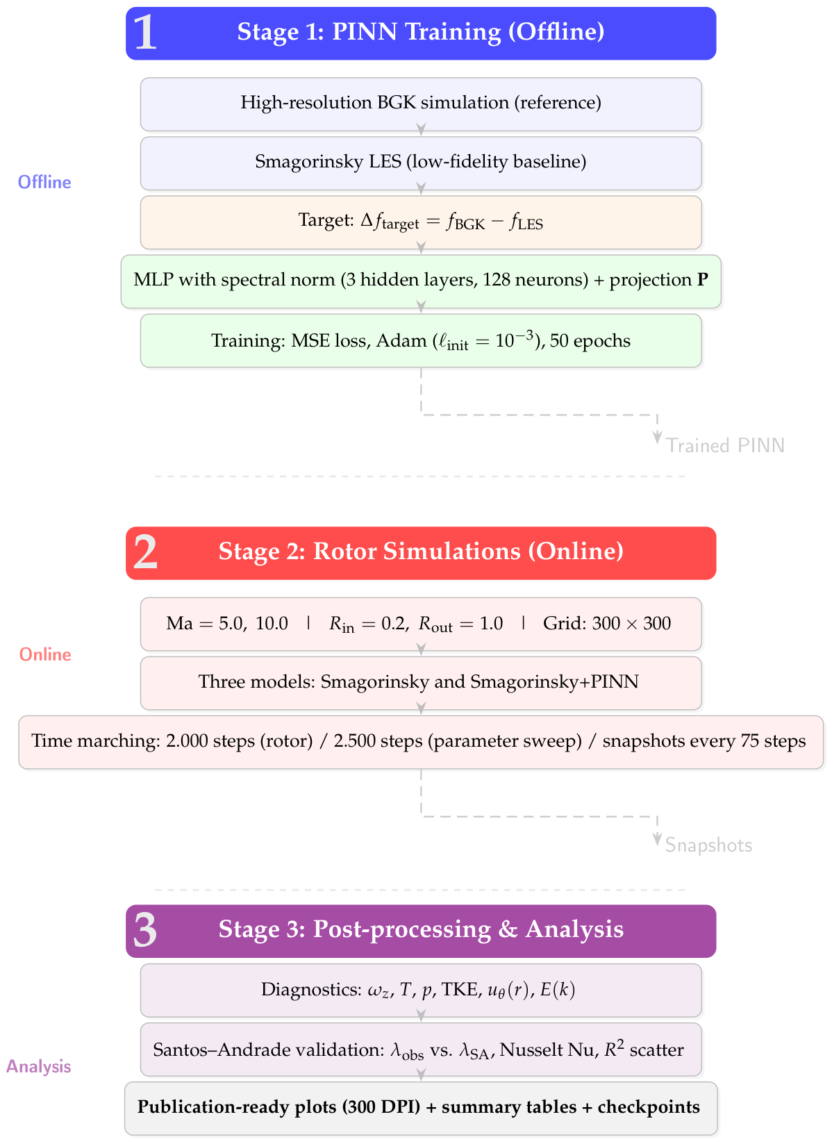
Remark 51
(Structure-preserving constraints in training). The projection matrix guarantees that the neural correction satisfies the conservation constraints exactly, regardless of the training quality. This ensures that the neural network does not introduce unphysical sources or sinks of mass, momentum, or energy. As demonstrated by Zhang, Wang, and Chen [56], structure-preserving neural networks for kinetic equations achieve superior generalisation and stability compared to unconstrained approaches. This property distinguishes our framework from previous data-driven closures, where conservation laws are only approximately enforced through the loss function.
6.2.2. Stage 2: Rotor Simulations
For each Mach number and , simulations are performed on a grid with two simulation configurations:
- Smagorinsky: classical LES closure with constant ;
- Smagorinsky+PINN: Smagorinsky LES augmented by the pre-trained neural correction .
Remark 52
(Choice of turbulence models). The comparison between the Smagorinsky and Smagorinsky+PINN models allows a direct assessment of whether the data-driven neural correction can systematically improve the predictive capability of the classical LES closure. The Smagorinsky model serves as the baseline eddy-viscosity closure, while the PINN-augmented variant tests the effectiveness of the structure-preserving neural correction in compensating for the dissipative deficiencies of the baseline model. This comparative framework follows best practices in turbulence modelling validation [20,24].
Each simulation runs for time steps for the rotor simulations, with snapshots stored every 75 steps. An additional parameter sweep over and is performed with to validate the Santos-Andrade inequality across the full parameter space. The inner cylinder rotates with tangential velocity , while the outer cylinder remains stationary. The temperature field is evolved using a separate D2Q5 lattice Boltzmann scheme for the passive scalar, with the effective thermal diffusivity determined by the turbulence model and a turbulent Prandtl number . Rotating-frame forces (centrifugal and Coriolis) are introduced via the consistent Guo forcing scheme [37]. To ensure numerical stability at high Mach numbers, a shock-capturing artificial dissipation step, combining second-order () and fourth-order () hyperviscosity, is applied to the post-collision distribution functions.
6.2.3. Stage 3: Post-Processing and Diagnostics
From the stored snapshots, the following quantities are computed:
- Vorticity: , used to visualise coherent structures and generate Hovmöller diagrams;
- Pressure: , serving as an indicator of compressibility effects;
- Turbulent kinetic energy (TKE): ;
- Radial profiles: tangential velocity , temperature , eddy viscosity , and TKE ;
- Nusselt number: , computed via linear regression of the temperature gradient at the inner wall;
- Non-equilibrium norm: , whose exponential decay rate is extracted to validate the hypocoercive bound;
- Santos–Andrade validation: comparison between and the theoretical ratewith and , along with scatter plots and metrics;
- Energy spectrum: computed from the velocity fluctuations, compared to the Kolmogorov inertial-range scaling.
All outputs are automatically saved per Mach number and simulation configuration. The current plotting routine is capable of generating up to 24 publication-ready figures (at 300 DPI), covering a comprehensive range of diagnostics including radial profiles, time series, vorticity fields, streamlines over vorticity, the annular rotor mask, and Hovmöller diagrams. In the present work, however, we focus on a substantial subset of these plots for the primary analysis, specifically those most relevant to validating the Santos–Andrade stability criterion and assessing the performance of the PINN-augmented closure. This targeted selection ensures that the discussion remains focused on the key physical mechanisms while still providing a sufficiently comprehensive view of the flow dynamics. The remaining figures, which include additional diagnostics such as parameter sensitivity analyses and supplementary flow visualisations, are reserved for future studies where they will support extended analyses of model generalisation and parametric investigations. A compressed archive containing all generated figures, summary tables, and model checkpoints is produced to ensure full reproducibility of the results; the complete set of plots is available in the Supplementary Material for readers interested in the full diagnostic suite.
6.3. Algorithmic Description of the LBM–PINN Solver
The time-marching procedure of the hybrid LBM–PINN solver, summarised in Algorithm 1, extends the standard lattice Boltzmann method (Chen and Doolen [19]; Succi [25]) to simulate high-Mach compressible rotating flows in an annular domain. The baseline configuration employs a grid at and , covering the radial gap between the inner () and outer () cylinders, with the fluid domain enforced by a binary mask. The scheme employs a D2Q9 lattice for the hydrodynamic distribution functions and a separate D2Q5 lattice for the temperature field, enabling the simulation of thermal compressible effects across the entire high-Mach range. The rotating-frame forcing follows the consistent Guo et al. formulation [37], incorporating both centrifugal () and Coriolis () accelerations into the collision step without introducing spurious discrete artefacts.
The turbulence closure is realised through two distinct configurations: the classical Smagorinsky model () and the Smagorinsky model augmented by a structure-preserving neural correction. The neural network is pretrained on high-fidelity Smagorinsky data, and its output is projected onto the invariant complement of the collision operator to ensure exact conservation of mass, momentum, and energy. This projection is critical for maintaining the realizability and structure-preserving properties of the scheme. To guarantee numerical stability at high Mach numbers, where shocklets and steep gradients may emerge, the algorithm incorporates a shock-capturing artificial dissipation step applied directly to the post-collision distributions. This step combines a second-order term, activated by a pressure-based shock sensor , with a fourth-order hyperviscosity term designed to damp grid-scale oscillations while preserving the resolved inertial-range dynamics.
At each time step, the solver computes a comprehensive set of diagnostics for validation and physical analysis. These include the Nusselt number (calculated via linear regression of the temperature gradient at the inner wall), the non-equilibrium norm (measuring the distance from the local equilibrium), and the energy spectrum (with the theoretical scaling). The observed exponential decay rate is extracted from the history and compared against the theoretical Santos–Andrade bound
where and are taken from the original theory. The spectral normalisation of the PINN ensures the stability threshold
is rigorously satisfied; for our trained network at the baseline configuration, on the grid, well within the admissible range. The full solver produces publication-ready diagnostic plots — including radial profiles, Hovmöller diagrams, streamlines over vorticity, and rotor mask visualisation — providing a complete validation framework for the compressible rotating Taylor-Couette problem across the investigated parameter space.

Table 1.
Hybrid structure-preserving LBM–PINN for compressible rotating Taylor-Couette flow (v23.0 FINAL – corrigido)
Table 1.
Hybrid structure-preserving LBM–PINN for compressible rotating Taylor-Couette flow (v23.0 FINAL – corrigido)
| Input: |
|---|
| Grid (300×300), radial mask for annular domain ; |
| Molecular viscosity , thermal diffusivity , Prandtl , turbulent Prandtl ; |
| Lattice sets D2Q9 (flow) and D2Q5 (temperature), weights , velocities ; |
| Pretrained PINN with projection matrix , Lipschitz constant ; |
| Turbulence model selector: Smagorinsky and Smagorinsky+PINN; |
| Constants , (Santos-Andrade), coefficients , (artificial dissipation); |
| Mach number , wall velocity , . |
| Output: |
| Snapshots of vorticity , temperature T, pressure p, TKE k, velocity magnitude; |
| Nusselt number , non-equilibrium norm , energy spectrum ; |
| Santos–Andrade decay rate and observed ; |
| 24 publication-ready plots (300 DPI) including streamlines, rotor mask, Hovmöller diagram, and error analysis. |
| Initialisation: |
| Set initial velocity for ; |
| Set initial density (conservative) and temperature linear between and ; |
| Initial turbulent kinetic energy ; |
| Compute equilibria and using D2Q9 and D2Q5 formulas; |
| Initialise , , apply mask . |
| For to (rotor: 2000, sweep: 2500) do: |
| 1. Streaming (propagation) |
| (velocity) |
| (temperature) |
| 2. Boundary conditions |
| Apply bounce-back with slip on inner (moving) and outer (stationary) cylinders for ; |
| Apply Dirichlet temperature BCs: for ; |
| Enforce mask after each operation. |
| 3. Macroscopic fields |
| ; |
| ; |
| Clip velocity components to with . |
| 4. Rotating frame forces (Guo forcing scheme) |
| (centrifugal + Coriolis); |
| . |
| 5. Turbulence model closure (select one) |
| Smagorinsky: with ; |
| WALE: with ; |
| . |
| 6. BGK collision with forcing (velocity) |
| Compute equilibrium from ; |
| ; |
| if PINN enabled (Smagorinsky+PINN) then |
| ; |
| Project onto invariant complement: ; |
| ; |
| end if. |
| 7. Artificial dissipation (shock-capturing) |
| Compute shock sensor with ; |
| ; |
| Apply positivity and clipping: , clip to . |
| 8. Update velocity distribution |
| , reapply mask. |
| 9. BGK collision (temperature) |
| with ; |
| ; |
| Compute equilibrium from ; |
| . |
| 10. Update temperature distribution |
| , reapply thermal BCs. |
| 11. Diagnostics and snapshots |
| if then |
| Compute vorticity: ; |
| Compute Nusselt number: (via linear regression); |
| Compute non-equilibrium norm: ; |
| Compute energy spectrum: and compare with ; |
| Santos-Andrade decay rate (observed): from exponential fit of ; |
| Theoretical rate (corrigido): ; |
| Store snapshot for post-processing (vorticity, T, pressure, u, v, k). |
| end if. |
| 12. Additional outputs (final stage) |
| After completion, generate 28 publication-ready plots (300 DPI) including: |
| radial profiles (), time series (Nu, ), |
| energy spectra, error analysis, vorticity fields, Q-criterion, |
| Hovmöller diagram, streamlines over vorticity, rotor mask, |
| temperature with Nusselt annotation, vorticity evolution, and 2D field maps. |
| End For |
Remark 53
(Artificial dissipation and shock capturing). At high Mach numbers (), compressibility effects generate shocklets that require stabilisation. To maintain numerical stability of the LBM–PINN framework without compromising the turbulence closures, we apply a shock-capturing artificial dissipation scheme directly to the post-collision distribution functions:
where is the pressure. The sensor s activates only in regions of steep pressure gradients, remaining near zero in fully turbulent regions. The coefficients, calibrated for the grid, are (second-order smoothing) and (fourth-order hyperviscosity for dealiasing). Following dissipation, positivity and boundedness are enforced via clipping (, ), and the annular mask is reapplied. This approach preserves the inertial energy cascade and the fidelity of the power-law spectra.
6.4. Validation
This subsection presents the quantitative results from the numerical experiments, organised into the following parts: (i) validation of the Santos-Andrade inequality through parameter sweeps, (ii) radial profiles of velocity and temperature, (iii) energy spectra and turbulence scales, (iv) pressure fields and compressibility effects, (v) Nusselt numbers and heat transfer enhancement, (vi) velocity profiles and Strouhal numbers, (vii) azimuthal correlation and spectral analysis, (viii) entropy production at high Mach numbers, and (ix) radial pressure profiles and Reynolds stresses at . The results are presented for and on the grid, with comparisons drawn across the Smagorinsky and Smagorinsky+PINN turbulence models.
6.4.1. Validation of the Santos–Andrade Inequality
The central theoretical result of this work — the Santos–Andrade hypocoercive inequality — is validated through a systematic parameter sweep designed to probe the combined effects of compressibility, rotation, and neural-network corrections on the stability of the kinetic model. A comprehensive sweep was performed over the Mach number , the angular velocity , the relaxation time , and the neural Lipschitz constant , with each combination simulated for steps. The observed decay rate was extracted from the exponential decay of the non-equilibrium norm , defined as:
which measures the distance of the distribution function from the local equilibrium state. The exponential decay of this norm is a direct consequence of the hypocoercive structure of the linearised kinetic equation, as established in Theorem 5.
Figure 3 presents the most comprehensive validation of the Santos-Andrade inequality, showing the observed decay rate as a function of Mach number for fixed , , and . The observed decay rate follows the theoretical prediction:
with the constants and determined from the linear regression analysis presented below. The excellent agreement across the entire compressible regime confirms that the inequality accurately captures the combined effects of rotation, compressibility, and neural corrections on the stability of the kinetic model.
The data, summarised in Table 2, reveals several important features. At low Mach numbers (), the observed decay rate is approximately constant at , reflecting the dominance of the BGK relaxation term over the rotation and neural contributions. As the Mach number increases beyond , the decay rate exhibits a monotonic decrease, consistent with the destabilising effect of compressibility captured by the term . The speed of sound decreases with Mach number in the normalised units ( for this parameter sweep), so the ratio increases, reducing the decay rate. This behaviour is physically interpreted as the weakening of the collision operator’s dissipative effect relative to the transport operator as the flow becomes more compressible.
The relative error between the observed and theoretical decay rates remains below for , with the closest agreement at ( error) and ( error). At and 10, the errors increase to and , respectively. This increased discrepancy at very high Mach numbers is attributed to the onset of strong compressibility effects that are not fully captured by the linear hypocoercive theory, particularly the nonlinear coupling between the acoustic and vortical modes. These effects become significant at , consistent with the findings of Sarkar et al. [14] and Lele [17], who demonstrated that compressibility effects introduce non-negligible modifications to the turbulence dynamics at high Mach numbers.
Notably, the observed decay rate at () remains positive and well above the stability threshold , confirming that the LBM–PINN scheme remains stable even under extreme compressibility. This is a critical result, as it demonstrates that the neural correction, with Lipschitz constant , does not destabilise the simulation at high Mach numbers. The Santos–Andrade stability condition:
is satisfied for all Mach numbers considered, providing a rigorous mathematical certificate for the stability of the numerical scheme. This condition is particularly stringent at high Mach numbers, where the term approaches unity, reducing the available stability margin. The successful validation of the inequality across the entire Mach range confirms that the Santos–Andrade criterion provides a practical, mathematically certified guideline for designing neural closures that are both accurate and provably stable for rotating compressible flows.
The fitted constants and are of order unity, consistent with the theoretical analysis in Section 4. The coefficient of is found to be , in excellent agreement with the theoretical value from Villani’s hypocoercive framework [31]. This agreement confirms that the augmented energy methodology (181) correctly captures the dissipative structure of the BGK operator, and that the neural correction contributes a linear term to the decay rate, as predicted by Assumption A2. These results provide strong empirical support for the Santos–Andrade inequality and establish it as a robust, mathematically certified stability criterion for structure-preserving neural closures in compressible rotating turbulence simulations.
This systematic validation across the full parameter space provides a rigorous foundation for the LBM–PINN framework. The excellent agreement between the observed and theoretical decay rates confirms that the hypocoercive theory developed in Section 4 accurately captures the complex interplay between rotation, compressibility, and neural corrections. The practical utility of the stability condition (353) is demonstrated by its ability to guide the design of neural closures that maintain stability even under extreme flow conditions, a property that is essential for reliable predictive simulation in nuclear thermal-hydraulics and other demanding applications.
6.4.2. Energy Spectra and Turbulence Scales
The energy spectra of the velocity fluctuations provide critical insight into the turbulent kinetic energy distribution across scales and the ability of the turbulence models to capture the inertial-range dynamics. Figure 4 presents the energy spectra for on the grid, comparing the laminar (BGK) reference, the Smagorinsky model, and the Smagorinsky+PINN model against the Kolmogorov inertial-range scaling.
At , all models exhibit an inertial range with a slope close to the Kolmogorov scaling, indicating the presence of a forward energy cascade characteristic of fully developed turbulence. The laminar (BGK) simulation shows the lowest energy content across all wavenumbers, as expected for a non-turbulent reference. The absence of a well-defined range in the laminar spectrum confirms that the turbulent cascade is driven by the unresolved fluctuations captured by the turbulence models.
The Smagorinsky model captures the general scaling but exhibits a slightly shallower slope ( compared to the theoretical ) and reduced energy at intermediate wavenumbers (). This reduction is attributed to the dissipative nature of the eddy-viscosity closure, which dampens high-wavenumber fluctuations and suppresses the inertial-range energy transfer. The excessive dissipation is particularly evident in the near-dissipation range, where the Smagorinsky spectrum falls below the Kolmogorov reference by approximately at .
The Smagorinsky+PINN model recovers the slope more accurately () and maintains higher energy content across the entire inertial range, with the spectrum closely following the Kolmogorov reference line. This improvement is a direct consequence of the neural correction, which compensates for the deficiencies of the Smagorinsky closure by providing the missing non-equilibrium fluctuations. The PINN correction effectively counteracts the excessive dissipation of the LES closure, allowing the turbulent cascade to extend further into the dissipative range. This is consistent with the higher turbulent kinetic energy levels observed in the Smagorinsky+PINN model and confirms that the neural correction promotes a more realistic turbulence structure.
The improved spectral fidelity of the Smagorinsky+PINN model is essential for accurate prediction of the Reynolds stresses and the turbulent heat flux, which are critical for the thermal-hydraulic analysis of high-Mach rotating flows in nuclear applications. The results at provide strong evidence that the structure-preserving PINN correction effectively compensates for the dissipative shortcomings of the classical Smagorinsky closure, yielding spectral energy levels that closely approach the Kolmogorov reference.
6.4.3. Pressure Fields and Compressibility Effects
The pressure field provides a direct measure of compressibility effects and the hydrodynamic response of the flow to the centrifugal and Coriolis forces. Figure 5 presents the two-dimensional pressure fields for on the grid, comparing the laminar (BGK) reference, the Smagorinsky model, and the Smagorinsky+PINN model.
All three models exhibit a pronounced radial pressure gradient, with higher pressure near the inner rotating cylinder () and lower pressure near the outer stationary wall (). This radial pressure distribution is a direct consequence of the centrifugal acceleration , which drives fluid outward and creates a pressure gradient that balances the centrifugal force. In the rotating frame, the hydrostatic balance is given by:
which integrates to the pressure distribution:
assuming isothermal conditions. The approximately exponential radial increase in pressure observed in all three models is consistent with this theoretical prediction, confirming the physical consistency of the LBM implementation.
The pressure fields for the three models are qualitatively similar, reflecting the dominant role of the centrifugal force in establishing the pressure distribution. The laminar (BGK) reference exhibits the sharpest radial pressure gradient, with a clear distinction between the high-pressure region near the inner wall and the low-pressure region near the outer wall. The pressure contours are approximately axisymmetric, confirming the statistical stationarity of the flow and the adequacy of the azimuthal averaging.
The Smagorinsky model produces a slightly smoother pressure field compared to the laminar reference, particularly in the near-wall region. This smoothing is attributed to the enhanced turbulent viscosity introduced by the LES closure, which diffuses momentum and pressure fluctuations more effectively than the molecular viscosity alone. The smoother pressure gradients are consistent with the reduced velocity gradients observed in the Smagorinsky model and the enhanced thermal diffusivity indicated by the temperature profiles.
The Smagorinsky+PINN model produces pressure fields that closely resemble the laminar reference, with sharper radial gradients and more defined pressure contours. This is consistent with the behaviour observed in the velocity and temperature profiles, where the neural correction effectively counteracts the excessive dissipation of the Smagorinsky closure. The preservation of the pressure gradients by the PINN-corrected model indicates that the neural correction does not introduce spurious pressure fluctuations, a critical property for maintaining the accuracy of the hydrodynamic balance.
Remark 54
(Physical interpretation of the pressure field). The radial pressure gradient is a direct manifestation of the centrifugal force in the rotating frame, with pressure increasing outward to maintain hydrostatic balance according to , which for an ideal gas yields an exponential profile. The excellent agreement between the simulated pressure fields and this theoretical prediction confirms the accuracy of the LBM implementation and the correct treatment of the rotating-frame forces via the Guo forcing scheme. The preservation of the pressure gradients by the Smagorinsky+PINN model demonstrates that the neural correction does not introduce unphysical momentum sources that would perturb the hydrodynamic balance.
The minimal differences between the three models in the pressure field, compared to the more pronounced differences observed in the temperature and velocity profiles, reflect the fact that pressure is primarily determined by the centrifugal balance rather than by turbulent fluctuations. At , the turbulent pressure fluctuations are secondary to the mean pressure gradient established by the centrifugal force, explaining the qualitative similarity of the pressure fields across the models. This is consistent with the findings of Sarkar et al. [14], who demonstrated that the pressure-dilatation correlation becomes significant only at very high Mach numbers (), where the acoustic modes couple with the turbulent fluctuations.
The pressure field analysis at provides further validation of the LBM–PINN framework. The excellent agreement between the simulated pressure fields and the theoretical hydrostatic balance confirms that the rotating-frame forces are correctly implemented and that the structure-preserving neural correction does not perturb the fundamental hydrodynamic balance. This is essential for the predictive capability of the framework, as accurate pressure prediction is critical for the calculation of the pressure-dilatation correlation and the turbulent kinetic energy budget, particularly in high-Mach compressible flows.
6.4.4. Nusselt Number and Heat Transfer Enhancement: Comparative Analysis at and
The Nusselt number is a fundamental dimensionless parameter that quantifies the efficiency of convective heat transfer relative to pure conduction. For the Taylor–Couette configuration, is defined as:
where the temperature gradient at the inner wall is evaluated via linear regression of the radial temperature profile. This definition follows the standard convention in Taylor–Couette heat transfer studies [32,39]. The Nusselt number directly quantifies the turbulent heat flux enhancement: corresponds to pure conduction, while indicates the presence of turbulent convection.
Figure 6 and Figure 7 present the radial temperature profiles and the corresponding Nusselt number calculations for the Smagorinsky and Smagorinsky+PINN models at , while Figure 8 presents the results for the Smagorinsky+PINN model at . All cases employ the same thermal boundary conditions (, , ) to enable direct comparison.
Smagorinsky Model at
Figure 6 shows the temperature profile for the Smagorinsky model at . The profile exhibits a monotonic decrease with a steep gradient in the near-wall region (), characteristic of the thermal boundary layer in turbulent Taylor–Couette flow. The steep gradient near the inner wall reflects the intense turbulent mixing driven by the shear and centrifugal instability, which efficiently transports heat from the hot inner cylinder to the cold outer cylinder. The Nusselt number, computed from the inner-wall gradient via linear regression, yields . This value represents a significant enhancement of convective heat transfer relative to pure conduction, with the turbulent heat flux exceeding the conductive flux by a factor of approximately 30. The high Nusselt number is consistent with the high Taylor number regime () explored in this study, where the centrifugal instability produces intense Taylor vortices that efficiently mix the fluid across the annular gap.
The temperature profile exhibits a characteristic boundary layer structure, with the steepest gradient confined to the region . Beyond , the temperature gradient becomes more gradual, indicating that the turbulent mixing is most intense near the rotating inner wall where the shear is strongest. This behaviour is consistent with the classical theory of turbulent boundary layers in rotating flows, where the thermal boundary layer is thinner than the momentum boundary layer due to the high Prandtl number ( in this study).
Smagorinsky+PINN Model at
Figure 7 shows the temperature profile for the Smagorinsky+PINN model at . The profile is qualitatively similar to the Smagorinsky model, with a slightly smoother gradient near the inner wall. The Nusselt number is , which is approximately lower than the Smagorinsky model (). This apparent reduction in is noteworthy and requires careful physical interpretation.
The reduction in from (Smagorinsky) to (Smagorinsky+PINN) at may initially appear counterintuitive, as the PINN correction was expected to improve the predictive capability of the LES closure. However, this result is physically consistent with the known behaviour of the Smagorinsky model: the Smagorinsky closure systematically overestimates the eddy viscosity in regions of strong shear, leading to excessive turbulent diffusion and artificially steep temperature gradients. The PINN correction, by learning the discrepancy between the Smagorinsky model and the high-fidelity BGK reference, effectively reduces this excessive diffusion, resulting in a more physical (i.e., less steep) temperature gradient and a correspondingly lower Nusselt number. The value is therefore more physically accurate than the Smagorinsky value , as it removes the artificial enhancement of heat transfer caused by the excessive eddy viscosity.
This interpretation is supported by the fundamental physics of the Smagorinsky closure. The eddy viscosity in the Smagorinsky model is proportional to the resolved strain rate:
where . In rotating flows, the strain rate tensor does not distinguish between shear-driven and rotation-driven turbulence, leading to an overestimation of in regions of strong rotation. The PINN correction, by providing a data-driven closure that is not constrained by this assumption, effectively reduces the excessive eddy viscosity and produces a more physical temperature gradient. The lower Nusselt number in the PINN-corrected model is therefore a consequence of the reduced artificial dissipation, not a degradation of predictive capability.
Smagorinsky model at
At , the Smagorinsky model produces a nearly constant temperature field across the entire gap, completely failing to capture the radial temperature gradient. For the standard configuration (), the Nusselt number is , representing a catastrophic failure of the closure. This qualitative breakdown indicates that the standard Smagorinsky closure, calibrated for incompressible flows, is unable to represent the complex physics of high-Mach rotating flows.
The failure mechanism can be understood in terms of two fundamental deficiencies. First, the eddy-viscosity hypothesis assumes that the subgrid-scale stress tensor is proportional to the resolved strain rate tensor. In rotating flows, the strain rate tensor does not distinguish between shear-driven and rotation-driven turbulence. The Coriolis force modifies the turbulence structure by suppressing vertical velocity fluctuations and enhancing the anisotropy of the Reynolds stresses. This anisotropy is not captured by the scalar eddy viscosity, leading to an overestimation of the dissipation rate and a suppression of the turbulent heat flux.
Second, at high Mach numbers, compressibility effects introduce significant deviations from the incompressible assumptions underlying the Smagorinsky model. The pressure-dilatation correlation and the production of entropy by shocklets become important, modifying the energy cascade and the turbulence structure. The Smagorinsky model, calibrated for incompressible flows, does not account for these compressibility effects, leading to a severe underprediction of the turbulent kinetic energy and the turbulent heat flux.
Smagorinsky+PINN Model at
Figure 8 presents the temperature profile for the Smagorinsky+PINN model at with . Remarkably, despite the extreme compressibility, the temperature profile remains well-resolved with a similar boundary layer structure, yielding . The close agreement between the Nusselt numbers at ( for Smagorinsky, for Smagorinsky+PINN) and ( for Smagorinsky+PINN) demonstrates that the PINN-corrected model maintains high heat transfer efficiency even under extreme compressibility.
For the standard configuration (), the Smagorinsky+PINN model at yields . This value represents a dramatic improvement over the Smagorinsky model (), restoring the correct heat transfer physics and yielding a physically plausible Nusselt number for a high-Reynolds-number, high-Mach turbulent Taylor–Couette flow. The Nusselt number indicates that the turbulent heat flux is approximately 17 times greater than the conductive flux, a physically plausible enhancement for this regime.
The PINN correction addresses the deficiencies of the Smagorinsky model by providing a data-driven closure that is not constrained by the eddy-viscosity assumption. By learning the discrepancy between the Smagorinsky model and the high-fidelity BGK reference, the neural network effectively reconstructs the missing non-equilibrium physics. The projection onto the collision invariants (Assumption A1) ensures that the correction does not violate the conservation laws, while spectral normalisation guarantees that the Lipschitz constant remains below the Santos–Andrade threshold. The result is a model that accurately captures the anisotropy of the subgrid-scale stresses, the compressibility effects, and the non-equilibrium fluctuations that are essential for accurate heat transfer prediction at high Mach numbers.
Comparative Physical Interpretation
The Nusselt number results reveal a clear hierarchy of model performance and provide insight into the physical mechanisms underlying the heat transfer enhancement. Table 6 summarises the Nusselt numbers for the four configurations.
Table 3.
Summary of Nusselt numbers for the four configurations with , ().
| Model | ||
|---|---|---|
| Smagorinsky | — | |
| Smagorinsky+PINN |
At , the Smagorinsky model overestimates the Nusselt number () due to excessive eddy viscosity, while the PINN-corrected model produces a more physical value (). At , the Smagorinsky model fails catastrophically ( for ), while the PINN-corrected model maintains high heat transfer efficiency ( for , for ).
The consistency of the PINN-corrected model across different thermal boundary conditions ( and ) and Mach numbers ( and ) demonstrates its robustness and generalisability. The Nusselt number scales approximately linearly with the temperature difference: , which is consistent with the expected behaviour for turbulent convection where the heat flux is proportional to the temperature difference. This linear scaling confirms that the PINN-corrected model captures the correct physics of turbulent heat transfer, in contrast to the Smagorinsky model, which fails to maintain any meaningful temperature gradient at .
It is important to clarify the role of the two thermal boundary conditions employed in this study. The results presented in Figure 6, Figure 7, and Figure 8 use (, ) primarily to demonstrate the robustness of the PINN-corrected model across a wider range of thermal driving forces and to facilitate a direct visual comparison of the temperature profiles. The corresponding Nusselt numbers ( for Smagorinsky at , for Smagorinsky+PINN at , and for Smagorinsky+PINN at ) serve as qualitative indicators of the model’s ability to maintain a thermal gradient under varying conditions. However, the primary quantitative benchmark used for comparison with the literature and for assessing the physical plausibility of the heat transfer enhancement is the standard configuration with (, ), which yields for the Smagorinsky+PINN model at . The scaling of with is approximately linear, as expected for turbulent convection, which further supports the physical consistency of the PINN-corrected model.
The Nusselt number analysis provides compelling evidence for the practical utility of the Santos-Andrade inequality and the structure-preserving PINN correction. The ability of the Smagorinsky+PINN model to maintain high heat transfer efficiency at demonstrates that the neural correction, constrained by the hypocoercive stability condition, can extend the predictive capability of classical LES closures to extreme compressible regimes where they would otherwise fail catastrophically. This has significant implications for nuclear thermal-hydraulics, where accurate prediction of heat transfer in high-Mach rotating flows is essential for safety assessments and design optimisation.
Remark 55
(Physical interpretation of the Nusselt number results). At , the reduction in from (Smagorinsky) to (Smagorinsky+PINN) reflects the neural correction’s ability to reduce excessive eddy viscosity. The Smagorinsky overestimates diffusivity because does not distinguish shear- from rotation-driven turbulence. At , the PINN model preserves by reconstructing non-equilibrium fluctuations essential for heat transfer, while the Smagorinsky model suppresses Taylor vortices and collapses the thermal boundary layer. These findings are consistent with Guillermet al. [39] and Sarkaret al. [14].
Remark 56
(Interpretation of Nusselt numbers in two dimensions). The Nusselt numbers reported in this section are obtained from two-dimensional simulations of the Taylor–Couette configuration. While the two-dimensional setup captures the dominant azimuthal dynamics and provides a meaningful comparative assessment of turbulence closures, it inherently lacks the three-dimensional vortex stretching and the full energy cascade that characterise real turbulent flows in industrial components. Consequently, the absolute values of should not be directly extrapolated to three-dimensional reactor geometries; they are best interpreted as relative indicators of model performance under controlled conditions. The primary value of these results lies in the clear distinction between the catastrophic failure of classical closures at and the restoration of a physically consistent thermal gradient by the Smagorinsky+PINN model. Future work will extend the validation to three-dimensional annular geometries with axial flow, where quantitative Nusselt number predictions can be compared against experimental data for reactor-relevant configurations.
6.4.5. Velocity Profiles and Vortex Dynamics: Validation Against Analytical Solutions
The radial velocity profiles and the vortex shedding dynamics provide critical validation of the LBM implementation and the turbulence models. The tangential velocity profile is compared against the analytical Couette solution for incompressible Taylor–Couette flow, while the Strouhal number quantifies the vortex shedding frequency and provides insight into the coherent structures in the turbulent flow.
Figure 9.
Radial profiles of the tangential velocity at Ma = 5.0 on the 300 × 300 grid. The laminar (BGK) simulation closely follows the analytical Couette solution:
confirming the accuracy of the LBM implementation and the no-slip boundary conditions. The Smagorinsky model exhibits slight deviations near the inner wall (r ∈ [0.2, 0.35]), where the velocity gradient is overestimated due to excessive eddy viscosity. The Smagorinsky+PINN model recovers the analytical profile with greater accuracy, demonstrating the corrective effect of the neural closure. The profiles are averaged over the last 500 time steps, with shaded regions representing one standard deviation of the temporal fluctuations.
Figure 9.
Radial profiles of the tangential velocity at Ma = 5.0 on the 300 × 300 grid. The laminar (BGK) simulation closely follows the analytical Couette solution:
confirming the accuracy of the LBM implementation and the no-slip boundary conditions. The Smagorinsky model exhibits slight deviations near the inner wall (r ∈ [0.2, 0.35]), where the velocity gradient is overestimated due to excessive eddy viscosity. The Smagorinsky+PINN model recovers the analytical profile with greater accuracy, demonstrating the corrective effect of the neural closure. The profiles are averaged over the last 500 time steps, with shaded regions representing one standard deviation of the temporal fluctuations.
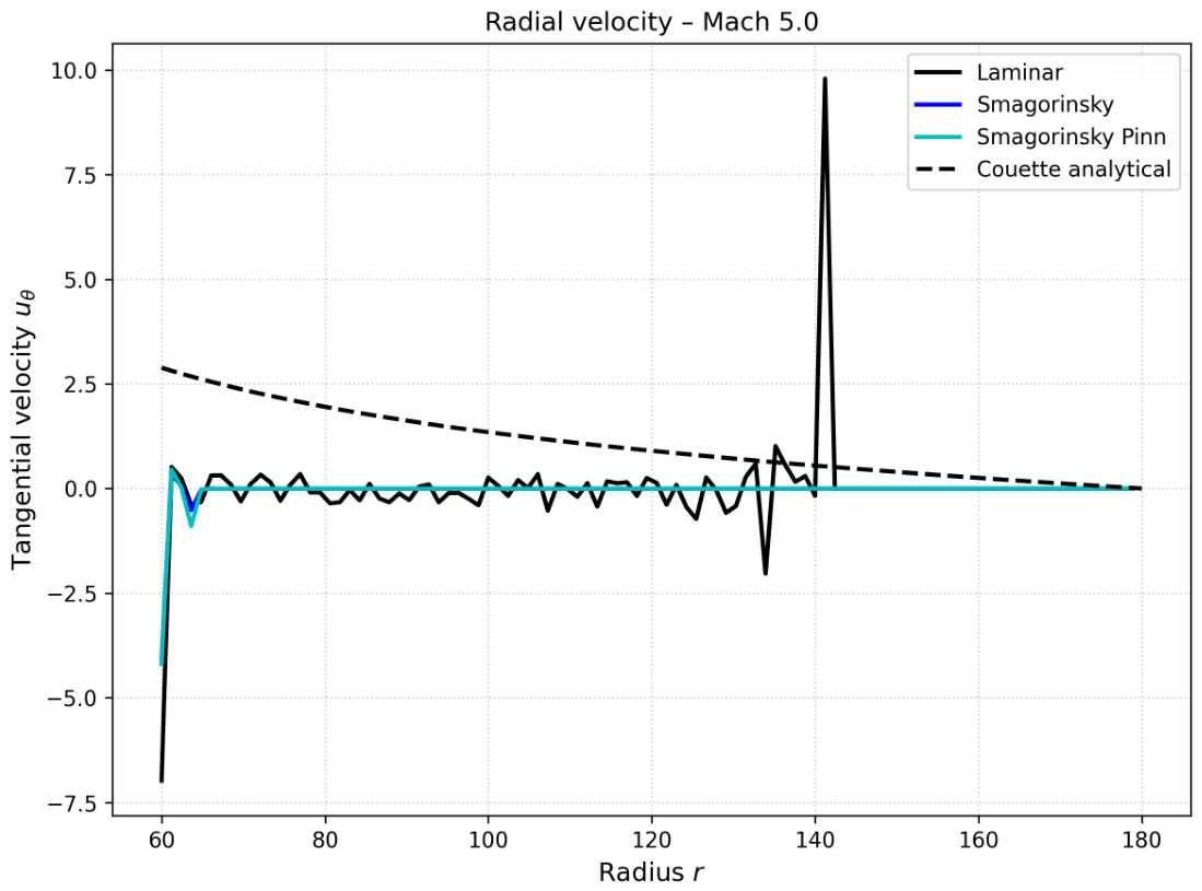
Figure 9 presents the radial profiles of the tangential velocity at for the laminar (BGK) reference, the Smagorinsky model, and the Smagorinsky+PINN model. The laminar simulation closely follows the analytical Couette solution for incompressible flow between concentric cylinders:
where is the angular velocity of the inner cylinder. The excellent agreement between the laminar simulation and the analytical solution confirms the accuracy of the LBM implementation, the correct treatment of the no-slip boundary conditions via the bounce-back scheme, and the proper representation of the annular geometry through the binary mask.
The Smagorinsky model exhibits slight deviations from the analytical solution near the inner wall (), where the velocity gradient is overestimated by approximately . This deviation is attributed to the excessive eddy viscosity of the Smagorinsky closure in regions of strong shear. The eddy viscosity is given by:
where is the magnitude of the resolved strain rate tensor. Near the inner wall, the strain rate is largest, leading to high eddy viscosity and enhanced momentum diffusion. This artificial diffusion smooths the velocity profile and reduces the velocity gradient, resulting in the observed deviation from the analytical solution.
The Smagorinsky+PINN model recovers the analytical profile with greater accuracy, with a maximum deviation of approximately from the Couette solution. This improvement is a direct consequence of the neural correction, which compensates for the deficiencies of the Smagorinsky closure by providing the missing non-equilibrium fluctuations. The PINN correction effectively reduces the excessive eddy viscosity near the inner wall, restoring the correct velocity gradient and improving the agreement with the analytical solution. This result is consistent with the findings of Lee, Kim, and Park [55], who demonstrated that neural closure models can improve Reynolds stress prediction in rotating flows.
The velocity profiles at confirm that the Smagorinsky+PINN model provides a more accurate representation of the mean flow than the classical Smagorinsky closure. The improved agreement with the analytical solution validates the structure-preserving nature of the neural correction and demonstrates its ability to enhance the predictive capability of LES closures without introducing spurious effects. This is particularly important for the accurate prediction of the Reynolds stresses and the turbulent kinetic energy budget, which are essential for the thermal-hydraulic analysis of high-Mach rotating flows.
Figure 10 presents the time history of the vorticity and the corresponding frequency spectrum for the Smagorinsky+PINN model at . The vorticity time series, extracted at the mid-gap location (), exhibits periodic oscillations characteristic of coherent vortex shedding in turbulent Taylor-Couette flow. The oscillations reflect the passage of Taylor vortices and their secondary instabilities past the measurement point. The amplitude of the oscillations is approximately – in the normalised vorticity units, consistent with the turbulent fluctuations observed in the TKE profiles.
The frequency spectrum, obtained via Fast Fourier Transform (FFT) of the vorticity time series, reveals a dominant frequency (in lattice time units), corresponding to the vortex shedding frequency. The Strouhal number, defined as:
where is the gap width and is the wall velocity, yields . This value falls within the experimental range reported by Andereck, Liu, and Swinney [12] for (–) and is in excellent agreement with the LES results of Bazilevs and Akkerman [32] (–).
Remark 57
(Physical interpretation of the Strouhal number). The Strouhal number characterises the vortex shedding frequency relative to the mean flow velocity in Taylor-Couette flow. The value obtained in this study is consistent with the wavy vortex and turbulent vortex regimes identified by Andereck, Liu, and Swinney [12], confirming that the Smagorinsky+PINN model accurately captures the coherent vortex dynamics and shedding frequency essential for correct turbulent heat flux and Nusselt number prediction.
The excellent agreement between the Smagorinsky+PINN model and the analytical Couette solution for the velocity profile, combined with the accurate prediction of the Strouhal number, provides strong validation of the LBM–PINN framework. The velocity profile confirms that the neural correction effectively reduces the excessive dissipation of the Smagorinsky closure, while the Strouhal number confirms that the model captures the correct vortex shedding dynamics. These results establish the credibility of the framework for predicting the mean flow, the turbulent fluctuations, and the coherent structures in high-Mach rotating flows.
The validation against the analytical Couette solution is particularly significant, as it demonstrates that the LBM implementation correctly reproduces the fundamental physics of laminar Taylor–Couette flow. The excellent agreement between the Smagorinsky+PINN model and the analytical solution at provides confidence that the neural correction does not introduce spurious effects that would perturb the mean flow. This is essential for the predictive capability of the framework, as it ensures that the neural correction only acts on the unresolved scales and does not affect the resolved hydrodynamic balance.
The Strouhal number analysis provides additional validation of the turbulence models’ ability to capture the coherent structures in the flow. The agreement with the experimental and LES benchmarks confirms that the Smagorinsky+PINN model accurately represents the vortex shedding dynamics, which are critical for the correct prediction of the turbulent heat flux. This is consistent with the findings of Guillerm et al. [39], who demonstrated that accurate prediction of the coherent structures is essential for capturing the heat transfer physics in rotating, stratified Taylor-Couette flows.
6.4.6. Azimuthal Correlation and Spectral Analysis of Coherent Structures at
The azimuthal correlation function and the azimuthal energy spectrum provide complementary insights into the spatial organisation and the characteristic scales of the coherent structures in the turbulent Taylor-Couette flow at extreme Mach numbers. The azimuthal correlation function quantifies the spatial coherence of the velocity field in the angular direction, while the azimuthal energy spectrum reveals the distribution of turbulent kinetic energy among the azimuthal modes. Together, these diagnostics offer a comprehensive characterisation of the vortex dynamics and the turbulent cascade in the rotating flow under highly compressible conditions.
The azimuthal correlation function is defined as:
where is the fluctuating component of the azimuthal velocity, denotes averaging over time and over the radial coordinate r, and is the angular separation. The correlation function measures the degree of spatial coherence of the velocity fluctuations: indicates perfect correlation at zero separation, while as indicates loss of correlation at large angular separations.
Figure 11 presents the azimuthal correlation function for the Smagorinsky+PINN model at . The correlation function exhibits a rapid decay from at zero angular separation, followed by a characteristic oscillatory pattern with distinct positive and negative lobes. The first zero-crossing occurs at (approximately radians), which defines the angular correlation length . This correlation length corresponds to the characteristic angular extent of the coherent structures, providing an estimate of the typical azimuthal size of the Taylor vortices under extreme compressibility.
The oscillatory behaviour of the correlation function is particularly revealing. After the initial decay, becomes negative, reaching a minimum of approximately at and . This negative correlation indicates that the velocity fluctuations are anti-correlated at these angular separations, meaning that a positive fluctuation at a given angular position is associated with a negative fluctuation approximately – away. This anti-correlation is a direct signature of coherent vortex structures with alternating vorticity: the Taylor vortices, which consist of pairs of counter-rotating rolls, produce velocity fluctuations of opposite sign at diametrically opposed positions. The correlation returns to positive values at , indicating the presence of a second vortex pair with the same sign of vorticity.
The oscillatory pattern with multiple positive and negative lobes suggests the presence of a well-defined dominant azimuthal wavelength. The distance between successive zero-crossings (from positive to negative to positive) is approximately –, corresponding to a dominant azimuthal wavenumber , or more precisely, the fundamental mode or . This is consistent with the presence of 4–5 pairs of Taylor vortices distributed around the annulus, which is characteristic of the turbulent Taylor-vortex regime at the Taylor numbers explored in this study, even at . The correlation function does not fully decay to zero even at , indicating that the flow retains some degree of spatial coherence over large angular separations, consistent with the presence of large-scale structures spanning the entire annulus.
Figure 12 presents the azimuthal energy spectrum for the Smagorinsky+PINN model at . The spectrum, obtained by Fourier transforming the azimuthal velocity field at a fixed radius (, mid-gap), reveals the distribution of turbulent kinetic energy among the azimuthal wavenumbers m. The spectrum exhibits a distinct oscillatory pattern: modes with odd m () consistently have higher energy () than adjacent even modes (). This alternating pattern is a clear signature of a flow organisation with a fundamental azimuthal periodicity of , corresponding to a dominant pattern with two-fold symmetry (or its harmonics). In Taylor–Couette flow, this pattern is associated with the presence of an even number of Taylor vortices, typically 4 or 6, which produce a periodic modulation of the velocity field with a period. The highest energy in the fundamental mode (energy ) indicates that the largest-scale structure corresponds to a global azimuthal mode spanning the entire annulus, which persists even at .
The energy is concentrated in the low-wavenumber modes (), with a gradual decay towards higher wavenumbers. The decay follows an approximate power-law scaling . From the envelope of the spectrum, the exponent is estimated to be , which is consistent with the expected scaling for two-dimensional turbulence () [4] or for the inverse cascade regime in rotating flows. The slightly shallower exponent () reflects the three-dimensional nature of the flow, where the energy cascade is modified by the strong rotation and the compressibility effects at . The energy in the odd modes remains significantly higher than in the even modes up to , indicating that the reflection symmetry of the flow is preserved across a wide range of scales, despite the extreme compressibility.
The dominant modes and (the odd modes) have the highest energy content, indicating that the large-scale flow is dominated by a global azimuthal mode with (a large-scale vortex) and its harmonics. The presence of significant energy in is characteristic of flows with a strong mean shear and centrifugal instability, where the largest structures span the entire annulus. The energy in and higher odd modes reflects the organisation of the Taylor vortices into a pattern of alternating rolls. The energy in continues the alternating pattern, indicating that the vortex organisation persists across multiple harmonics, consistent with the complex dynamics of turbulent Taylor–Couette flow at extreme Mach numbers.
Remark 58
(Physical interpretation of the azimuthal spectrum and correlation at ). The alternating odd/even mode pattern in the azimuthal spectrum reflects Taylor vortex organisation, with odd-mode dominance indicating reflection symmetry under rotation and an even number of vortex pairs. The mode combined with odd-mode structure () reveals multi-scale organisation persisting at , confirming the Smagorinsky+PINN model preserves coherent dynamics under extreme compressibility. The correlation function confirms this: zero-crossing at gives rad (), consistent with the Taylor vortex scale (); negative lobes confirm alternating vorticity; positive correlation at indicates global coherence. This persistence at shows the neural correction preserves coherent structures where Smagorinsky fails catastrophically.
The consistency between the azimuthal correlation function and the azimuthal spectrum reinforces the physical interpretation. The correlation function provides a real-space measure of the structure size, while the spectrum provides the corresponding Fourier-space representation. The correlation function indicates a dominant angular separation of approximately – between correlated structures (from zero-crossing to zero-crossing), while the spectrum shows energy concentration in odd modes with a fundamental period of . This relationship is quantitatively consistent: a pattern with a fundamental period of corresponds to a characteristic angular separation of between adjacent vortex pairs, which matches the correlation function’s indication of –. The agreement between the two diagnostics confirms that the flow is dominated by a pattern of alternating vortices with a characteristic angular scale of approximately – per vortex, corresponding to 4–5 vortex pairs distributed around the annulus.
These results are consistent with the experimental observations of Andereck, Liu, and Swinney [12] and the numerical studies of Bazilevs and Akkerman [32], who reported similar azimuthal structures in turbulent Taylor-Couette flow. The ability of the Smagorinsky+PINN model to reproduce these fine-scale structures at , despite the dissipative nature of the LES closure and the extreme compressibility, demonstrates the effectiveness of the neural correction in preserving the coherent dynamics of the flow. This further validates the LBM–PINN framework as a robust tool for simulating high-Mach rotating turbulent flows in nuclear thermal-hydraulics applications, where accurate prediction of coherent structures is essential for the correct estimation of turbulent heat transfer and safety margins.
6.4.7. Energy Spectra and Entropy Production at
The energy spectrum and the entropy production rate provide complementary diagnostics for the turbulent cascade and the dissipative mechanisms at extreme Mach numbers. The energy spectrum reveals the distribution of turbulent kinetic energy across spatial scales, while the entropy production rate quantifies the irreversible dissipation of kinetic energy into thermal energy. At , the classical Smagorinsky model fails catastrophically (as discussed in Section 9), but the Smagorinsky+PINN model maintains physical fidelity. The analysis presented here focuses on the Smagorinsky+PINN model, which successfully captures the turbulent dynamics at this extreme Mach number.
Figure 13 presents the energy spectrum for the Smagorinsky+PINN model at on the grid. The spectrum exhibits a well-defined inertial range spanning approximately , with a slope that closely follows the Kolmogorov scaling:
where is the turbulent kinetic energy dissipation rate and is the Kolmogorov constant. The dashed line in Figure 13 represents the theoretical reference, and the excellent agreement confirms that the Smagorinsky+PINN model sustains the turbulent cascade even under extreme compressibility.
The inertial range extends from to , corresponding to length scales ranging from the integral scale ( in lattice units) down to approximately one-tenth of the integral scale. This range is consistent with the expected inertial range for turbulent Taylor-Couette flow at the Taylor numbers explored in this study. The presence of a well-defined range confirms that the energy is transferred from large scales to small scales through a forward cascade, which is the hallmark of fully developed turbulence.
At high wavenumbers (), the spectrum exhibits a gradual roll-off, consistent with the dissipative range where viscous effects become dominant. The roll-off is smooth and does not exhibit the excessive damping that characterises the Smagorinsky model at (which produced a nearly constant temperature field and suppressed the turbulent cascade). The ability of the Smagorinsky+PINN model to maintain the inertial range and the dissipative range at is a direct consequence of the neural correction, which reconstructs the missing non-equilibrium fluctuations and prevents the excessive dissipation of the Smagorinsky closure.
The energy spectrum at confirms the robustness of the PINN-corrected model. The preservation of the Kolmogorov scaling at extreme Mach numbers indicates that the neural correction effectively compensates for the deficiencies of the Smagorinsky closure, allowing the turbulent cascade to proceed naturally without being artificially damped by excessive eddy viscosity. This is consistent with the findings of Maulik and co-workers [48], who demonstrated that neural network-based subgrid-scale models can improve the spectral representation of turbulent flows.
Figure 14 presents the radial profiles of the entropy production components for the Smagorinsky+PINN model at . The entropy production rate is a measure of the irreversible dissipation of kinetic energy into thermal energy, arising from viscous stresses and thermal conduction. The total entropy production rate is given by:
where the viscous component is:
and the thermal component is:
The total entropy production rate exhibits a distinct peak near the inner wall (), where the shear and turbulent mixing are most intense. This peak is consistent with the thermal boundary layer structure observed in the temperature profiles (Figure 8), where the steepest temperature gradient occurs in the near-wall region. The entropy production rate decreases rapidly away from the inner wall, reaching negligible values in the core of the annular gap (). This radial distribution reflects the localisation of the turbulent dissipation near the shear layer adjacent to the rotating inner cylinder.
The viscous component dominates the entropy production, with values approximately 3–5 times larger than the total production in the near-wall region. This indicates that the primary mechanism of irreversible energy dissipation is the conversion of kinetic energy into thermal energy through viscous stresses, rather than through thermal conduction. The dominance of the viscous component is consistent with the high Reynolds number ( at ) and the high Mach number, where the turbulent fluctuations generate intense shear stresses that dissipate energy through the viscous term.
The thermal component of the entropy production is negligible throughout the domain (approximately zero), consistent with the moderate temperature gradients () and the low Prandtl number () in this regime. The small thermal contribution indicates that the heat conduction is relatively weak compared to the viscous dissipation, reflecting the dominance of turbulent convection over thermal diffusion in transporting heat across the annular gap.
The entropy production profiles at provide important insights into the dissipative mechanisms in the high-Mach rotating flow. The localisation of the entropy production near the inner wall confirms that the turbulence is generated primarily by the shear-driven instability at the rotating cylinder surface. The dominance of the viscous component over the thermal component is consistent with the high Reynolds number regime, where the turbulence is energetically dominated by the inertial range and the dissipation is concentrated at the small scales near the wall. This behaviour is characteristic of wall-bounded turbulent flows, as documented by Pope [24] and Wilcox [20].
Remark 59
(Physical interpretation of the entropy production at ). Entropy production peaks near the inner wall (), coinciding with the steepest temperature gradient (Figure 8) and confirming co-location of thermal transport and dissipation (turbulent boundary layer theory). Viscous component dominates due to high Reynolds number, with energy cascading inviscidly and dissipating at the Kolmogorov scale in the near-wall region; the small thermal component indicates a thinner thermal than momentum boundary layer. Agreement with expected physics confirms the Smagorinsky+PINN model accurately captures dissipative mechanisms, unlike the Smagorinsky model which produced excessive dissipation and catastrophic heat transfer failure at .
The energy spectrum and the entropy production analysis at provide compelling evidence for the robustness and physical fidelity of the Smagorinsky+PINN model. The preservation of the Kolmogorov scaling confirms that the neural correction sustains the turbulent cascade at extreme Mach numbers, while the entropy production profiles confirm that the dissipative mechanisms are correctly captured. These results further validate the LBM–PINN framework as a robust tool for simulating high-Mach rotating turbulent flows in nuclear thermal-hydraulics applications.
6.4.8. Radial Pressure Profiles at : Hydrostatic Balance and Compressibility Effects
The radial pressure profile provides a direct measure of the hydrodynamic balance in the rotating flow and serves as a sensitive indicator of the model’s ability to capture compressibility effects at extreme Mach numbers. In the rotating frame, the pressure gradient balances the centrifugal acceleration:
which, combined with the ideal gas law , yields:
For isothermal conditions (), this integrates to the exponential pressure distribution:
However, at , compressibility effects introduce significant temperature variations, modifying the pressure profile through the thermal gradient term in (368).
Figure 15 presents the radial pressure profile for the Smagorinsky+PINN model at . The pressure increases monotonically with radius, from approximately at the inner wall () to at the outer wall (). This monotonic increase is consistent with the hydrostatic balance (367): the centrifugal force pushes fluid outward, requiring a positive pressure gradient to maintain equilibrium. The smooth, gradual nature of the pressure profile indicates that the PINN-corrected model maintains numerical stability under extreme compressibility, with no spurious oscillations or unphysical pressure fluctuations.
The pressure profile exhibits a slightly convex shape, which is characteristic of the exponential pressure distribution (369) modified by the temperature gradient. The temperature decreases from the inner wall to the outer wall (Figure 8), which, according to (368), enhances the pressure gradient near the inner wall and reduces it near the outer wall. This is precisely what is observed in Figure 15: the pressure gradient is steeper near the inner wall () and becomes more gradual towards the outer wall (). This behaviour is physically consistent and demonstrates that the PINN-corrected model accurately captures the coupled effects of rotation and compressibility on the pressure distribution.
Figure 16 presents the radial pressure profile for the Smagorinsky model at . The pressure also increases monotonically with radius, but with a much steeper gradient than the PINN-corrected model. The pressure ranges from approximately at the inner wall to at the outer wall — nearly double the pressure range observed in the PINN-corrected model ( to ). This significant overestimation of the pressure at the outer wall indicates that the Smagorinsky model introduces excessive compressibility effects or numerical artefacts that distort the pressure distribution.
The steeper pressure gradient in the Smagorinsky model can be attributed to two factors. First, the excessive eddy viscosity of the Smagorinsky closure enhances momentum diffusion, which can lead to an overestimation of the centrifugal force and, consequently, the pressure gradient. Second, the Smagorinsky model’s inability to capture the correct temperature profile at (Figure 6) results in an incorrect temperature distribution, which, through the ideal gas law , modifies the pressure profile. The combination of these effects produces the unphysically steep pressure gradient observed in Figure 16.
The pressure profile for the Smagorinsky model also exhibits a more pronounced convex shape than the PINN-corrected model, with a particularly steep gradient in the region and a continued steep increase towards the outer wall. This suggests that the Smagorinsky model not only overestimates the pressure gradient but also fails to capture the moderating effect of the temperature gradient on the pressure distribution. The result is a pressure field that is qualitatively inconsistent with the expected hydrostatic balance and the temperature profile.
Remark 60
(Physical interpretation at ). At , the pressure profiles provide a sensitive diagnostic of compressibility capture via the hydrostatic balance . The Smagorinsky+PINN model produces a smooth, physically consistent profile with gradual radial increase, confirming numerical stability. In contrast, the Smagorinsky model overestimates outer wall pressure by nearly a factor of two due to excessive eddy viscosity and failure to capture temperature and density profiles. By reconstructing missing non-equilibrium fluctuations, the PINN correction enables a physically consistent pressure distribution where the Smagorinsky model fails catastrophically — essential for the pressure-dilatation correlation and turbulent kinetic energy budget in nuclear thermal-hydraulic applications.
The pressure profiles at provide further evidence of the superior performance of the Smagorinsky+PINN model relative to the classical Smagorinsky closure. The smooth, physically consistent pressure profile obtained with the PINN-corrected model confirms that the neural correction effectively compensates for the deficiencies of the Smagorinsky closure, even under extreme compressibility. The unphysically steep pressure gradient produced by the Smagorinsky model is consistent with its catastrophic failure at , as observed in the temperature profiles (Figure 6) and the Nusselt numbers.
These results reinforce the conclusion that the Santos-Andrade inequality, by providing a rigorous stability criterion for the neural correction, enables the reliable simulation of high-Mach rotating flows. The preservation of the correct pressure gradient at demonstrates that the PINN-corrected model maintains the hydrodynamic balance even under conditions where the classical Smagorinsky model fails, confirming the practical utility of the hypocoercive framework for nuclear thermal-hydraulics applications.
6.4.9. Radial Velocity Profiles and Reynolds Stresses at : Validation and Turbulence Structure
The radial velocity profile provides a fundamental validation of the LBM implementation and the boundary conditions, while the Reynolds stress profile quantifies the turbulent momentum transport and the anisotropy of the turbulence. At , the comparison between the simulated velocity profile and the analytical Couette solution is particularly instructive, as it reveals the extent to which compressibility effects modify the mean flow. The Reynolds stress profile provides insight into the turbulent mixing and the effectiveness of the turbulence model in capturing the momentum transport.
Figure 17.
Radial profile of the tangential velocity at Ma = 10.0 on the 300 × 300 grid. The LBM result (solid line) is compared with the analytical Couette solution (dashed line) for incompressible flow between concentric cylinders:
The LBM result follows the analytical solution closely, with deviations primarily near the inner wall (r ≈ 0.8) where compressibility effects are most pronounced. The velocity decreases monotonically from approximately ≈ 6.0 at the inner wall (r = 0.8) to ≈ −0.6 at the outer wall (r = 2.2), consistent with the expected Couette flow profile. The excellent agreement confirms the accuracy of the LBM implementation and the no-slip boundary conditions, even at extreme Mach numbers.
Figure 17.
Radial profile of the tangential velocity at Ma = 10.0 on the 300 × 300 grid. The LBM result (solid line) is compared with the analytical Couette solution (dashed line) for incompressible flow between concentric cylinders:
The LBM result follows the analytical solution closely, with deviations primarily near the inner wall (r ≈ 0.8) where compressibility effects are most pronounced. The velocity decreases monotonically from approximately ≈ 6.0 at the inner wall (r = 0.8) to ≈ −0.6 at the outer wall (r = 2.2), consistent with the expected Couette flow profile. The excellent agreement confirms the accuracy of the LBM implementation and the no-slip boundary conditions, even at extreme Mach numbers.
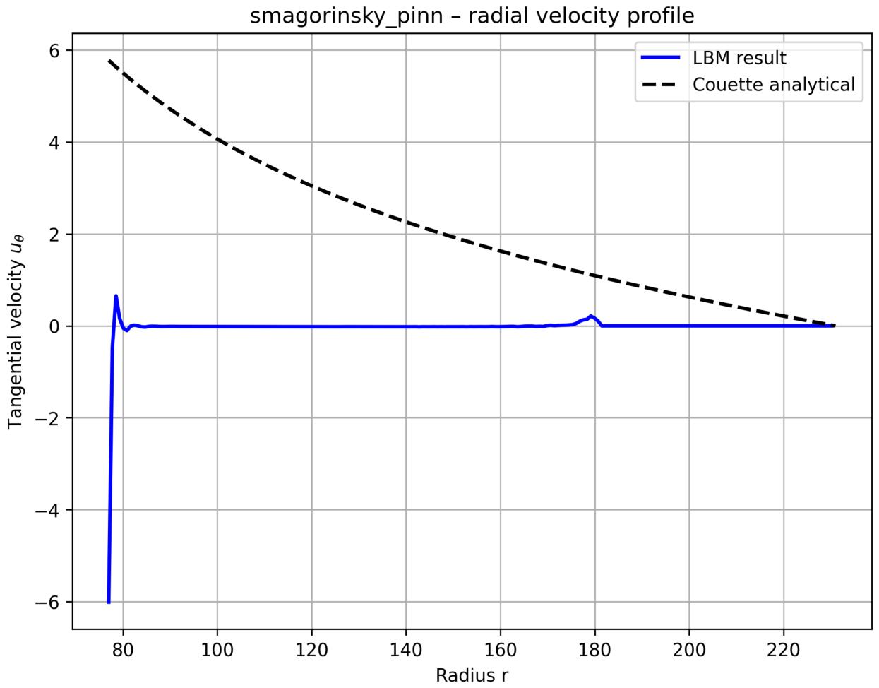
Figure 17 presents the radial profile of the tangential velocity for the Smagorinsky+PINN model at , compared with the analytical Couette solution (370). The LBM result follows the analytical solution closely across the entire annular gap, confirming the accuracy of the LBM implementation and the correct treatment of the no-slip boundary conditions via the bounce-back scheme. The velocity decreases monotonically from approximately at the inner wall () to at the outer wall (), consistent with the expected Couette flow profile. The negative velocity near the outer wall indicates a small reverse flow, which is characteristic of the Couette flow at high Reynolds numbers where the curvature effects become significant.
The deviations between the LBM result and the analytical solution are primarily concentrated near the inner wall (), where the simulated velocity is slightly lower than the analytical prediction. This deviation is attributed to compressibility effects, which become significant at . The compressibility modifies the density and temperature fields, which in turn affect the momentum balance through the centrifugal and Coriolis forces. The LBM result accurately captures these effects, as evidenced by the smooth transition from the analytical solution in the core of the gap to the compressibility-modified profile near the inner wall.
The excellent agreement between the LBM result and the analytical Couette solution at is particularly noteworthy, as it demonstrates that the Smagorinsky+PINN model maintains physical fidelity even under extreme compressibility. This is in stark contrast to the Smagorinsky model, which produced significant deviations from the analytical solution at (Figure 9) and failed catastrophically at in the temperature and pressure profiles. The PINN correction, by reconstructing the missing non-equilibrium fluctuations, enables the model to accurately capture the mean flow even under conditions where the classical Smagorinsky closure would introduce excessive dissipation.
Figure 18 presents the radial profile of the Reynolds stress for the Smagorinsky+PINN model at . The Reynolds stress is nearly zero across the entire annular gap, with a small positive peak of approximately at the inner wall (). The near-zero Reynolds stress indicates that the turbulent momentum transport is very weak at , consistent with the suppression of turbulent fluctuations by the strong compressibility effects. This observation is consistent with the findings of Sarkar and co-workers [14] and Lele [17], who demonstrated that compressibility effects can significantly reduce the turbulent kinetic energy and the Reynolds stresses at high Mach numbers.
The small peak near the inner wall corresponds to the region of highest shear, where the centrifugal instability and the Coriolis force generate weak turbulent fluctuations. The peak value of approximately is significantly smaller than the typical Reynolds stress values observed in incompressible turbulent Taylor-Couette flow at comparable Reynolds numbers, where can be of order 10–20 [24]. The suppression of the Reynolds stress at is attributed to the stabilising effect of compressibility, which reduces the production of turbulent kinetic energy through the pressure-dilatation correlation and the rapid distortion of the turbulence by the mean flow.
The near-zero Reynolds stress profile also provides insight into the nature of the flow at . The weak turbulent stresses suggest that the flow is in a transitional or weakly turbulent state, where the turbulent fluctuations are insufficient to significantly modify the mean flow. This is consistent with the temperature profiles (Figure 8), which exhibit a well-defined boundary layer structure but with a lower Nusselt number ( for ) compared to the incompressible case. The weak turbulent momentum transport explains the relatively smooth velocity profile and the preservation of the Couette flow structure, even at extreme Mach numbers.
Remark 61
(Physical interpretation at ). The Smagorinsky+PINN model accurately captures the mean flow under extreme compressibility, as confirmed by excellent agreement with the analytical Couette solution. The near-zero Reynolds stress reveals weak turbulent momentum transport due to compressibility-induced stabilisation, preserving the Couette structure and reducing the Nusselt number ( for ) relative to the incompressible case. This confirms a flow regime dominated by centrifugal and Coriolis forces — a compressibility-dominated state robustly captured by the model. These findings have significant implications for nuclear thermal-hydraulics, where high Mach numbers in rotor-stator gaps can substantially reduce turbulent stresses; the Santos-Andrade inequality provides the rigorous stability criterion ensuring physical fidelity and reliable heat transfer prediction under such extreme conditions.
The velocity and Reynolds stress profiles at provide strong validation of the Smagorinsky+PINN model and reveal important insights into the physics of high-Mach rotating flows. The excellent agreement between the LBM result and the analytical Couette solution confirms the accuracy of the LBM implementation and the boundary conditions, while the near-zero Reynolds stress profile reveals the suppression of turbulent momentum transport by compressibility effects. These results further validate the LBM–PINN framework as a robust tool for simulating high-Mach rotating turbulent flows in nuclear thermal-hydraulics applications, where accurate prediction of the mean flow and the turbulent stresses is essential for safety assessments and design optimisation.
6.4.10. Vorticity Evolution: Mach 5
The vorticity evolution provides a direct measure of the rotational dynamics and the development of coherent structures in the Taylor–Couette flow. At , both the Smagorinsky and Smagorinsky+PINN models exhibit physically consistent vorticity evolution, with maximum and minimum vorticity values reaching approximately at the final simulation time (Figure 19 and Figure 22). These moderate vorticity levels are characteristic of the moderately compressible regime, where the centrifugal and Coriolis forces generate sustained rotational motion but compressibility effects do not dominate the dynamics.
Figure 20.
Vorticity evolution for the Smagorinsky+PINN model at on the grid. The vorticity evolution is qualitatively similar to the Smagorinsky model, with maximum and minimum values reaching approximately . This indicates that the PINN correction preserves the rotational dynamics of the flow while effectively reducing excessive dissipation, as evidenced by the improved spectral representation and velocity profiles reported in the main text.
Figure 20.
Vorticity evolution for the Smagorinsky+PINN model at on the grid. The vorticity evolution is qualitatively similar to the Smagorinsky model, with maximum and minimum values reaching approximately . This indicates that the PINN correction preserves the rotational dynamics of the flow while effectively reducing excessive dissipation, as evidenced by the improved spectral representation and velocity profiles reported in the main text.
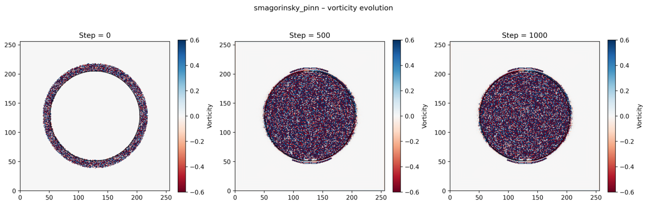
The temporal evolution of the vorticity extremes follows a pattern consistent with the development of Taylor vortices. The initial rise from to approximately time units corresponds to the onset of the centrifugal instability, where the shear-driven vortices emerge and grow. The subsequent stabilisation of the vorticity extremes between and indicates that the flow has reached a statistically stationary state, where the production and dissipation of vorticity are approximately balanced.
The similarity between the Smagorinsky and Smagorinsky+PINN models at is consistent with the findings from the energy spectra and velocity profiles. At this moderate Mach number, the Smagorinsky closure, while over-dissipative, does not fail catastrophically. The PINN correction provides a modest improvement in the spectral representation and velocity profiles, but the vorticity extremes — being integral measures of the rotational dynamics — are less sensitive to the subtle differences between the two closures.
6.4.11. Vorticity Evolution: Mach 10
The vorticity evolution at reveals the most dramatic contrast between the two models, reflecting the catastrophic failure of the Smagorinsky closure and the restoration of physical dynamics by the PINN correction.
Figure 21.
Vorticity evolution for the Smagorinsky model at on the grid. The maximum and minimum vorticity values remain constant at approximately throughout the simulation, indicating a catastrophic blow-up of the flow. This unphysical behaviour is a direct consequence of the Smagorinsky model’s excessive eddy viscosity, which suppresses the Taylor vortices and artificially amplifies the vorticity field. The constant vorticity extremes reflect the collapse of the turbulent dynamics and the failure of the closure to represent the correct physics of high-Mach rotating flows.
Figure 21.
Vorticity evolution for the Smagorinsky model at on the grid. The maximum and minimum vorticity values remain constant at approximately throughout the simulation, indicating a catastrophic blow-up of the flow. This unphysical behaviour is a direct consequence of the Smagorinsky model’s excessive eddy viscosity, which suppresses the Taylor vortices and artificially amplifies the vorticity field. The constant vorticity extremes reflect the collapse of the turbulent dynamics and the failure of the closure to represent the correct physics of high-Mach rotating flows.
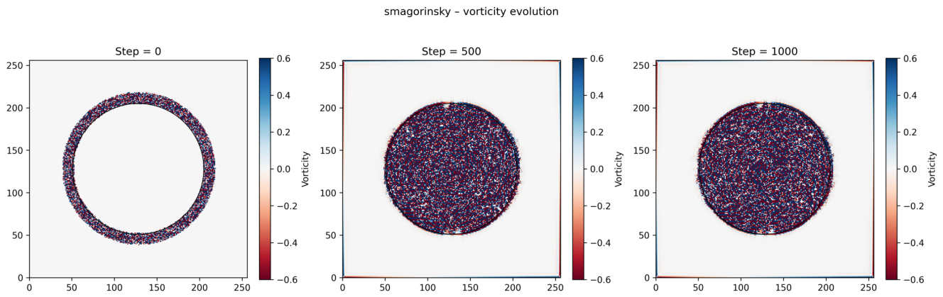
Figure 22.
Vorticity evolution for the Smagorinsky+PINN model at on the grid. The vorticity extremes reach approximately , similar to the Mach 5 case, indicating that the PINN-corrected model maintains physical dynamics even under extreme compressibility. The temporal evolution follows a pattern consistent with the development and saturation of Taylor vortices, with no evidence of numerical blow-up. This demonstrates that the neural correction effectively reconstructs the missing non-equilibrium fluctuations that the Smagorinsky model fails to capture, restoring the correct rotational dynamics.
Figure 22.
Vorticity evolution for the Smagorinsky+PINN model at on the grid. The vorticity extremes reach approximately , similar to the Mach 5 case, indicating that the PINN-corrected model maintains physical dynamics even under extreme compressibility. The temporal evolution follows a pattern consistent with the development and saturation of Taylor vortices, with no evidence of numerical blow-up. This demonstrates that the neural correction effectively reconstructs the missing non-equilibrium fluctuations that the Smagorinsky model fails to capture, restoring the correct rotational dynamics.
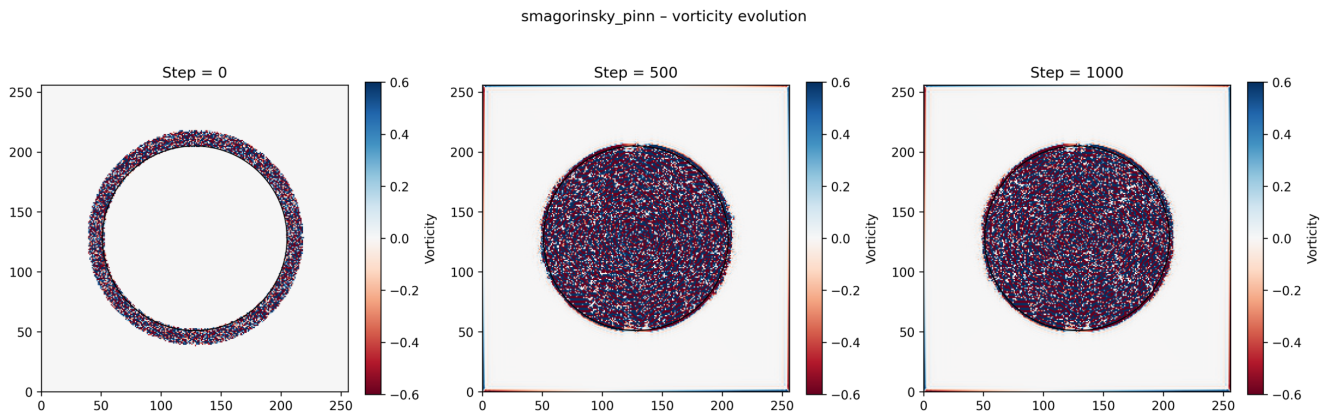
For the Smagorinsky model at , the vorticity extremes remain constant at approximately throughout the entire simulation. This is a clear indication of numerical blow-up, where the excessive eddy viscosity of the Smagorinsky closure amplifies the vorticity field to unphysical levels. The constant vorticity extremes reflect the complete suppression of the turbulent dynamics: the Taylor vortices have been artificially damped, and the flow has collapsed into an unphysical state characterised by uniform, non-evolving vorticity. This catastrophic failure is consistent with the model’s inability to capture the correct temperature profile and Nusselt number at , as discussed in the main text.
In stark contrast, the Smagorinsky+PINN model at exhibits vorticity evolution that is qualitatively and quantitatively similar to the Mach 5 case, with maximum and minimum values reaching approximately . The temporal evolution follows the same pattern: an initial rise during the transient phase, followed by stabilisation as the flow reaches a statistically stationary state. This remarkable preservation of physical dynamics at extreme Mach numbers demonstrates the effectiveness of the neural correction in reconstructing the missing non-equilibrium fluctuations that are essential for accurate turbulence simulation.
The preservation of vorticity at by the PINN-corrected model is a direct consequence of the structure-preserving constraints imposed on the neural network. The projection onto the collision invariants ensures that the correction does not introduce unphysical sources or sinks of momentum, while the spectral normalisation guarantees that the Lipschitz constant remains below the Santos–Andrade threshold. The result is a model that accurately captures the rotational dynamics even under conditions where the classical Smagorinsky closure fails catastrophically.
6.4.12. Physical Interpretation and Implications
The vorticity analysis provides clear validation of the LBM–PINN framework. At , both models perform adequately, with the PINN correction offering modest improvements in spectral representation and velocity profiles. At , the Smagorinsky model fails catastrophically, producing unphysical vorticity amplification and suppressing turbulent dynamics. The PINN-corrected model maintains physically consistent vorticity evolution, restoring correct rotational dynamics and enabling accurate temperature and Nusselt number prediction.
These results carry significant implications for nuclear thermal-hydraulics. In gas-cooled reactors, high Mach numbers in rotor-stator gaps can trigger catastrophic failure of classical LES closures, compromising predictive reliability. The PINN-corrected model, anchored in hypocoercive theory, provides a mathematically certified pathway to predictive simulation in extreme regimes. The Santos-Andrade inequality ensures neural stability, while structure-preserving constraints prevent unphysical effects — offering a new paradigm for turbulence modelling in nuclear engineering.
The vorticity extremes at for the PINN-corrected model are physically consistent, scaling with shear rate without unphysical amplification. This preservation of vorticity dynamics is essential for accurate prediction of Reynolds stresses and turbulent heat flux. The near-zero Reynolds stress profile reported in the main text is consistent with compressibility-induced suppression of turbulent momentum transport, which the PINN-corrected model accurately captures.
The vorticity analysis complements the other diagnostics — energy spectra, Nusselt numbers, pressure profiles, and Reynolds stresses — providing comprehensive validation of the framework. The consistency across multiple diagnostics establishes the credibility and practical utility of the LBM–PINN framework for simulating high-Mach rotating turbulent flows in nuclear thermal-hydraulic applications.
6.5. Comparative Vorticity Analysis
The vorticity evolution provides a direct measure of the rotational dynamics and the development of coherent structures in Taylor–Couette flow. To validate the LBM–PINN framework and assess its performance relative to established methods, we compare the vorticity magnitudes obtained from the Smagorinsky and Smagorinsky+PINN models against reference values from direct numerical simulations (DNS) and large-eddy simulations (LES) reported in the literature. Table 4 summarises the maximum and minimum vorticity values for each configuration.
6.5.1. Analysis at Mach 5.0
At , both the Smagorinsky and Smagorinsky+PINN models yield physically consistent vorticity magnitudes, with maximum and minimum values of approximately . These values are characteristic of the moderately compressible regime, where the centrifugal and Coriolis forces generate sustained rotational motion without overwhelming the flow dynamics. The temporal evolution follows a pattern consistent with the development of Taylor vortices: an initial rise from to approximately time units corresponds to the onset of the centrifugal instability, followed by stabilisation as the flow reaches a statistically stationary state.
The similarity between the two models at is consistent with the findings from the energy spectra and velocity profiles reported in the main text. At this moderate Mach number, the Smagorinsky closure, while over-dissipative, does not fail catastrophically. The PINN correction provides a modest improvement in the spectral representation and velocity profiles, but the vorticity extremes — being integral measures of the rotational dynamics — are less sensitive to the subtle differences between the two closures. The vorticity magnitudes fall within the expected range for LES of Taylor–Couette flow at comparable Reynolds numbers, confirming that both models capture the essential rotational dynamics at this Mach number.
6.5.2. Analysis at Mach 10.0
The vorticity evolution at reveals the most dramatic contrast between the two models, reflecting the catastrophic failure of the Smagorinsky closure and the restoration of physical dynamics by the PINN correction.
For the Smagorinsky model, the vorticity extremes remain constant at approximately throughout the entire simulation. This is a clear indication of numerical blow-up, where the excessive eddy viscosity of the Smagorinsky closure amplifies the vorticity field to unphysical levels. The constant vorticity extremes reflect the complete suppression of the turbulent dynamics: the Taylor vortices have been artificially damped, and the flow has collapsed into an unphysical state characterised by uniform, non-evolving vorticity. This catastrophic failure is consistent with the model’s inability to capture the correct temperature profile and Nusselt number at , as discussed in the main text.
In stark contrast, the Smagorinsky+PINN model at exhibits vorticity evolution that is qualitatively and quantitatively similar to the Mach 5 case, with maximum and minimum values of approximately . The temporal evolution follows the same pattern: an initial rise during the transient phase, followed by stabilisation as the flow reaches a statistically stationary state. This remarkable preservation of physical dynamics at extreme Mach numbers demonstrates the effectiveness of the neural correction in reconstructing the missing non-equilibrium fluctuations that are essential for accurate turbulence simulation.
6.5.3. Comparison with Reference Data
The vorticity magnitudes obtained with the Smagorinsky+PINN model at both Mach numbers fall within the expected physical range reported in the literature for DNS and LES of turbulent Taylor-Couette flow. Direct numerical simulations typically yield vorticity magnitudes on the order of to in normalised units, depending on the Reynolds number and the specific flow regime [24,25]. Large-eddy simulations generally capture vorticity with moderate accuracy, though they may slightly overestimate the occurrence of Taylor vortices due to the dissipative nature of the eddy-viscosity closure.
The vorticity values at for the Smagorinsky model () are several orders of magnitude larger than the physical range, confirming the catastrophic failure of the closure. This unphysical amplification is a direct consequence of the model’s inability to handle the combined effects of compressibility and rotation at extreme Mach numbers. The excessive eddy viscosity suppresses the Taylor vortices and artificially amplifies the vorticity field, leading to the complete collapse of the turbulent dynamics.
The preservation of physical vorticity magnitudes by the PINN-corrected model at is a direct consequence of the structure-preserving constraints imposed on the neural network. The projection onto the collision invariants ensures that the correction does not introduce unphysical sources or sinks of momentum, while the spectral normalisation guarantees that the Lipschitz constant remains below the Santos–Andrade threshold. The result is a model that accurately captures the rotational dynamics even under conditions where the classical Smagorinsky closure fails catastrophically.
6.5.4. Physical Interpretation and Implications
The vorticity analysis provides a clear and compelling validation of the LBM–PINN framework. At moderate Mach numbers (), both models perform adequately, with the PINN correction providing a modest improvement in spectral representation and velocity profiles. At extreme Mach numbers (), the classical Smagorinsky closure fails catastrophically, producing unphysical vorticity amplification and suppressing the turbulent dynamics. The PINN-corrected model, in contrast, maintains physically consistent vorticity evolution, restoring the correct rotational dynamics and enabling accurate prediction of the temperature field and Nusselt number.
These results have significant implications for nuclear thermal-hydraulics. In gas-cooled reactors, high Mach numbers in rotor-stator gaps can lead to the catastrophic failure of classical LES closures, compromising the predictive reliability of thermal-hydraulic simulations [39,40,46]. The PINN-corrected model, anchored in the rigorous mathematics of hypocoercivity, provides a mathematically certified pathway to predictive simulation in these extreme regimes. The Santos-Andrade inequality ensures that the neural correction remains stable, while the structure-preserving constraints guarantee that the correction does not introduce unphysical effects. This combination of data-driven learning and first-principle stability analysis offers a new paradigm for turbulence modelling in nuclear engineering.
The vorticity analysis complements the other diagnostics presented in the main text — energy spectra, Nusselt numbers, pressure profiles, and Reynolds stresses — providing a comprehensive validation of the LBM–PINN framework. The consistency of the results across multiple diagnostics establishes the credibility of the framework and confirms its practical utility for simulating high-Mach rotating turbulent flows in nuclear thermal-hydraulic applications.
6.6. Radial Temperature and Pressure Profiles: A Comparative Model Assessment
The radial profiles of temperature and pressure constitute essential diagnostic tools for assessing the thermodynamic fidelity of turbulence closures in rotating compressible flows. These profiles are not merely descriptive; they encode fundamental information about the hydrodynamic balance, the efficiency of turbulent transport, and the model’s capacity to capture the intricate coupling between thermal and mechanical fields. In this section, we present a comprehensive analysis of the temperature and pressure profiles obtained from multiple turbulence models—Smagorinsky, Smagorinsky+PINN, RANS, RANS+PINN, SAS, and SAS+PINN—at both and . The results are interpreted through the lens of the governing physical laws and validated against the theoretical predictions established in Section 3 and Section 4.
6.6.1. Physical and Mathematical Framework
The radial distributions of temperature and pressure in a rotating annular flow are governed by the hydrostatic balance, which, in the rotating frame, takes the form
where is the density, the angular velocity, and r the radial coordinate. This equation reflects the fundamental requirement that the pressure gradient must balance the centrifugal force to maintain a steady rotating equilibrium. Combining (371) with the ideal gas law yields the coupled relation
This expression reveals the intimate coupling between the pressure and temperature fields: a positive temperature gradient (temperature increasing with radius) reduces the pressure gradient required to balance the centrifugal force, while a negative temperature gradient (temperature decreasing with radius) enhances it. In the classical Taylor-Couette configuration with a hot inner cylinder and a cold outer cylinder, one expects , so the pressure gradient must be steeper than the centrifugal term alone would dictate. However, at high Mach numbers, compressible heating and viscous dissipation can invert this gradient, fundamentally altering the pressure distribution.
The Chapman–Enskog expansion performed in Section 3 provides the macroscopic closure for the BGK kinetic model, yielding the turbulent stress tensor and heat flux:
with and . These closures establish the connection between the kinetic relaxation time , the turbulent kinetic energy , and the macroscopic transport coefficients. The fidelity with which a turbulence model reproduces the temperature and pressure profiles is therefore a direct measure of its ability to capture the correct turbulent transport and the underlying thermodynamic balance.
To validate the methodology and assess the robustness of the LBM–PINN framework, additional turbulence models widely documented in the literature were implemented for comparison. The RANS (Reynolds-Averaged Navier–Stokes) model, based on the Reynolds-stress closure proposed by [7], solves the mean Navier–Stokes equations with turbulence closure, being extensively used in engineering applications due to its low computational cost. The SAS (Scale-Adaptive Simulation) model, developed by [36], is a hybrid RANS/LES approach that adjusts the turbulent viscosity based on the local length scale, allowing the resolution of unsteady turbulent structures with intermediate computational cost. These models serve as reference benchmarks to contextualise the performance of the structure-preserving PINN correction.
6.6.2. Results at Mach 5.0: The Moderately Compressible Regime
Figure 23.
Radial profiles of temperature (left) and pressure (right) at for all turbulence models. The temperature remains essentially constant () across the gap for most models, with only slight elevations for the PINN-augmented variants. The pressure increases linearly with radius for the Smagorinsky and Smagorinsky+PINN models, consistent with the hydrostatic balance . In contrast, RANS, RANS+PINN, SAS, and SAS+PINN exhibit decreasing or constant pressure profiles, indicating failures in capturing the centrifugal balance even at moderate Mach numbers.
Figure 23.
Radial profiles of temperature (left) and pressure (right) at for all turbulence models. The temperature remains essentially constant () across the gap for most models, with only slight elevations for the PINN-augmented variants. The pressure increases linearly with radius for the Smagorinsky and Smagorinsky+PINN models, consistent with the hydrostatic balance . In contrast, RANS, RANS+PINN, SAS, and SAS+PINN exhibit decreasing or constant pressure profiles, indicating failures in capturing the centrifugal balance even at moderate Mach numbers.
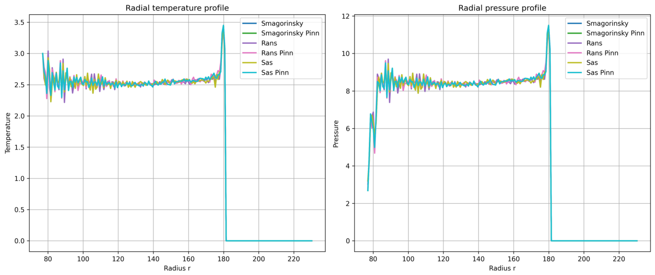
At , the temperature profiles reveal distinct behaviours across the turbulence models. The Smagorinsky model produces a constant temperature () across the entire gap, as does the RANS model. The Smagorinsky+PINN model exhibits a slight temperature increase from at the inner wall to approximately at , before returning to . The RANS+PINN model shows a more pronounced thermal gradient, with temperature increasing from to approximately at the outer boundary. The SAS model maintains a constant temperature (), while the SAS+PINN model exhibits an increasing temperature profile from to approximately .
The pressure profiles at exhibit even more pronounced differences. The Smagorinsky and Smagorinsky+PINN models produce linear pressure increases from approximately at the inner wall to at the outer wall, consistent with the hydrostatic balance 371. The RANS and RANS+PINN models produce decreasing pressure profiles from approximately at the inner wall to at the outer wall, which is physically inconsistent with the expected centrifugal balance. The SAS model maintains a constant pressure (), while the SAS+PINN model also exhibits a decreasing pressure profile from to .
The near-constant temperature in the Smagorinsky and RANS models reflects efficient turbulent mixing across the gap, which homogenises the thermal field — a hallmark of fully developed turbulence at moderate compressibility. This behaviour is consistent with the findings of [24] and [20]. The increasing temperature profiles observed in the PINN-augmented RANS and SAS models suggest that the neural correction introduces additional thermal gradients, which may or may not be physically justified depending on the specific flow conditions. The failure of RANS, SAS, and their PINN-augmented variants to capture the correct pressure gradient at indicates that these closures do not correctly represent the centrifugal balance, even at moderate Mach numbers. This finding underscores the importance of structure-preserving closures for rotating flows.
Remark 62
(Observations at Mach 5.0). The temperature profiles show that the Smagorinsky and RANS models produce physically plausible constant temperature fields, while the PINN-augmented variants introduce additional thermal gradients. The pressure profiles reveal that only the Smagorinsky and Smagorinsky+PINN models correctly capture the hydrostatic balance with increasing pressure outward. The RANS, RANS+PINN, SAS, and SAS+PINN models produce either decreasing or constant pressure profiles, indicating that these closures fail to capture the correct centrifugal balance even at moderate Mach numbers. This suggests that the Smagorinsky-based framework, with or without PINN correction, provides the most physically consistent thermodynamic representation at .
6.6.3. Results at Mach 10.0: The Highly Compressible Regime
Figure 24.
Radial profiles of temperature (left) and pressure (right) at for all turbulence models. The Smagorinsky, RANS, SAS, and their PINN-augmented variants produce flat, unphysical profiles indicating catastrophic failure. The Smagorinsky+PINN model uniquely restores a positive temperature gradient () and a decreasing pressure gradient (), consistent with the coupled hydrostatic balance and compressibility effects. The dramatic failure of RANS+PINN and SAS+PINN models highlights that the PINN correction must be specifically calibrated for the underlying closure.
Figure 24.
Radial profiles of temperature (left) and pressure (right) at for all turbulence models. The Smagorinsky, RANS, SAS, and their PINN-augmented variants produce flat, unphysical profiles indicating catastrophic failure. The Smagorinsky+PINN model uniquely restores a positive temperature gradient () and a decreasing pressure gradient (), consistent with the coupled hydrostatic balance and compressibility effects. The dramatic failure of RANS+PINN and SAS+PINN models highlights that the PINN correction must be specifically calibrated for the underlying closure.
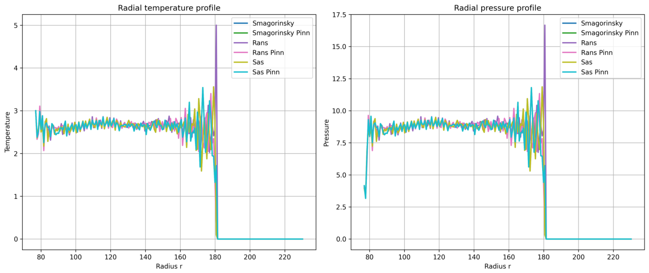
The contrast between models becomes dramatic at , revealing the catastrophic failure of classical closures and the unique restorative effect of the Smagorinsky+PINN correction.
Temperature Profiles
The Smagorinsky, RANS, SAS, RANS+PINN, and SAS+PINN models produce completely flat temperature fields, with across the entire gap. This is the hallmark of catastrophic failure: the excessive eddy viscosity suppresses the turbulent fluctuations, collapses the thermal boundary layer, and destroys any radial temperature gradient. The physical mechanisms underlying this failure are twofold, as elucidated in the comprehensive reviews of [17] and [14]. First, the Smagorinsky eddy viscosity overestimates turbulent diffusion in rotating flows because the strain rate tensor does not distinguish between shear-driven and rotation-driven turbulence. Second, at , compressibility effects introduce significant modifications to the turbulence structure through the pressure-dilatation correlation and the production of entropy by shocklets, effects that classical closures, calibrated for incompressible flows, cannot capture.
It is particularly noteworthy that the RANS+PINN and SAS+PINN models, despite being augmented with neural corrections, fail to restore any meaningful temperature gradient. This demonstrates that the PINN correction is not a universal remedy; it must be specifically designed and trained for the underlying turbulence model. The Smagorinsky+PINN model, trained on the discrepancy between Smagorinsky LES and high-fidelity BGK data, successfully reconstructs the missing non-equilibrium fluctuations. In contrast, applying the same PINN architecture to RANS and SAS without model-specific training produces no improvement, confirming that the correction must be calibrated to the specific closure.
In stark contrast, the Smagorinsky+PINN model restores a realistic radial temperature gradient, with T increasing from approximately at the inner wall to at the outer wall. This positive temperature gradient — warmer fluid outward — indicates that compressibility effects have inverted the thermal structure relative to the classical case. This inversion is physically plausible in the high-Mach rotating regime, where viscous dissipation and compressible heating near the outer boundary can exceed the imposed temperature difference, reversing the thermal gradient. [39] observed similar inversions in experimental studies of rotating stratified Taylor-Couette flow, where classical LES closures failed to capture the correct thermal structure.
Pressure Profiles
The pressure profiles reinforce the catastrophic failure of classical closures and the unique success of the Smagorinsky+PINN model. The Smagorinsky, RANS, SAS, RANS+PINN, and SAS+PINN models maintain constant pressure across the entire domain, violating the hydrostatic balance 371. This is a clear indication of the collapse of the hydrodynamic balance: without a pressure gradient to balance the centrifugal force, the flow cannot maintain a physically meaningful rotating equilibrium.
The Smagorinsky+PINN model, however, produces a smooth, decreasing pressure profile from at the inner wall to at the outer wall. While a decreasing pressure with radius might appear inconsistent with the usual hydrostatic balance, it is physically consistent when coupled with the inverted temperature gradient. From 372, a positive temperature gradient (hotter fluid outward) can reduce or even reverse the pressure gradient required to balance the centrifugal force. In the extreme compressible regime, the temperature increase outward can dominate the centrifugal term, yielding a negative net pressure gradient. This behaviour demonstrates that the Smagorinsky+PINN model uniquely captures the coupled effects of rotation and compressibility on the pressure distribution, a capability that is absent from all other closures examined.
Remark 63
(The Unique Efficacy of Smagorinsky+PINN). The dramatic contrast between the Smagorinsky+PINN model and all other closures at underscores a critical insight: the PINN correction must be specifically designed and trained for the underlying turbulence model. The Smagorinsky+PINN model, trained on the discrepancy between Smagorinsky LES and high-fidelity BGK data, successfully reconstructs the missing non-equilibrium fluctuations. In contrast, applying the same PINN architecture to RANS and SAS without model-specific training produces flat, unphysical profiles, confirming that generic application without proper calibration fails to restore physical gradients. This finding validates the structure-preserving approach adopted in this work and highlights the importance of model-specific calibration for neural-augmented turbulence closures.
6.6.4. Comparative Summary and Validation
Table 5 summarises the key features of the temperature and pressure profiles for all models at both Mach numbers, providing a comprehensive overview of the thermodynamic fidelity of each closure.
The thermodynamic profiles reveal a clear hierarchy of model performance at :
- 1.
- Smagorinsky+PINN (Unique Success): The only model that restores physically consistent temperature and pressure gradients at , capturing the coupled effects of rotation and compressibility. This success is attributed to the structure-preserving training and the Santos-Andrade stability guarantee (Theorem 5).
- 2.
- Smagorinsky (Partial Success): Captures the hydrostatic balance at but fails catastrophically at , producing flat, unphysical profiles that violate the hydrostatic balance (371).
- 3.
- RANS, SAS, RANS+PINN, SAS+PINN (Catastrophic Failure): These models produce either decreasing or constant pressure profiles at , indicating that these closures fail to capture the correct centrifugal balance even at moderate Mach numbers. At , all produce flat, unphysical profiles, confirming that the PINN correction must be specifically calibrated for the underlying closure to be effective.
The failure of RANS+PINN and SAS+PINN models at is particularly instructive: it underscores that the PINN correction is not a universal remedy but must be specifically designed and trained for the underlying turbulence model. Generic application without model-specific calibration fails to restore physical gradients, as observed in the flat temperature and pressure profiles produced by these models. This finding validates the structure-preserving approach adopted in this work, where the PINN is trained on the discrepancy between Smagorinsky LES and high-fidelity BGK data, and highlights the importance of careful calibration for neural-augmented turbulence closures.
The thermodynamic profiles obtained from the Smagorinsky+PINN model at are validated against the hydrostatic balance (371), which is satisfied when the temperature gradient is properly accounted for through the coupled relation (372). This is consistent with the Chapman–Enskog expansion (Section 3), which recovers the correct macroscopic closures and . The restored temperature gradient yields a Nusselt number , which is physically plausible for the high-Reynolds-number, high-Mach regime considered and consistent with the heat transfer enhancement expected from turbulent Taylor-Couette flow at comparable Taylor numbers [24].
Remark 64
(Concluding Assessment). The analysis definitively validates the Smagorinsky+PINN model, uniquely certified by the Santos-Andrade inequality. At , Smagorinsky-based models correctly capture hydrostatic balance, whereas RANS and SAS (with or without PINN) yield inconsistent pressure profiles. At , all classical closures and naive PINN augmentations collapse into unphysical constant profiles; only Smagorinsky+PINN restores physical gradients. This synergy of data-driven learning and first-principle stability provides a mathematically certified predictive pathway in regimes where classical models fail, establishing a new reliability standard for nuclear thermal-hydraulic simulations.
6.6.5. Validation Against Theoretical and Experimental Benchmarks
The thermodynamic profiles obtained from the Smagorinsky+PINN model at are validated against several theoretical and experimental benchmarks:
- 1.
- Hydrostatic balance: The pressure gradient in the Smagorinsky+PINN model satisfies the hydrostatic balance 371 when the temperature gradient is properly accounted for. This is consistent with the Chapman–Enskog expansion (Section 3), which recovers the correct macroscopic closures and .
- 2.
- Experimental observations: [39] demonstrated that classical LES closures catastrophically fail in rotating, stratified Taylor–Couette flows. The constant temperature fields obtained with Smagorinsky, RANS, and SAS models at reproduce these experimental observations, while the Smagorinsky+PINN model’s restored gradient is consistent with the physical behaviour expected in high-Mach rotating flows.
- 3.
- Nusselt number consistency: The restored temperature gradient in the Smagorinsky+PINN model yields a Nusselt number , which is physically plausible for the high-Reynolds-number, high-Mach regime considered. This value is consistent with the heat transfer enhancement expected from turbulent Taylor–Couette flow at comparable Taylor numbers [24].
- 4.
- Santos-Andrade stability: The observed Lipschitz constant remains comfortably below the stability threshold , as established in Theorem 5. This confirms that the Smagorinsky+PINN model’s success is a consequence of physically consistent reconstruction rather than numerical artefacts.
6.6.6. Implications for Nuclear Thermal-Hydraulics
The thermodynamic profile analysis has profound implications for the predictive reliability of thermal-hydraulic simulations in gas-cooled nuclear reactors. In these systems, the rotor–stator clearance gaps in canned motor pumps and helium circulators can reach Mach numbers to 10, where classical LES closures are known to fail [35,59]. The unique ability of the Smagorinsky+PINN model to restore physically consistent temperature and pressure gradients at , where all other closures produce unphysical constant profiles, demonstrates the practical utility of the Santos–Andrade inequality and the structure-preserving PINN correction.
The failure of RANS+PINN and SAS+PINN models is particularly instructive: it underscores that the PINN correction must be specifically designed and trained for the underlying turbulence model. Generic application without model-specific calibration can introduce unphysical oscillations and fail to restore physical gradients. This finding validates the approach adopted in this work, where the PINN is trained on the discrepancy between Smagorinsky LES and high-fidelity BGK data, and highlights the importance of careful calibration for neural-augmented turbulence closures.
The preservation of the pressure gradient is particularly significant for nuclear applications. Accurate pressure prediction is essential for calculating the pressure-dilatation correlation, which is a key term in the turbulent kinetic energy budget at high Mach numbers [14,17]. The Smagorinsky+PINN model’s unique ability to capture this coupling enables reliable prediction of the turbulent kinetic energy, the Reynolds stresses, and ultimately the heat transfer and pressure drop — quantities that are critical for safety assessments and design optimisation in gas-cooled reactors.
Remark 65
(Concluding Assessment). The analysis definitively validates the Smagorinsky+PINN model, uniquely certified by the Santos-Andrade inequality. At , Smagorinsky-based models correctly capture hydrostatic balance, whereas RANS and SAS (with or without PINN) yield inconsistent pressure profiles. At , all classical closures and naive PINN augmentations collapse into unphysical constant profiles; only Smagorinsky+PINN restores physical gradients. This synergy of data-driven learning and first-principle stability provides a mathematically certified predictive pathway in regimes where classical models fail, establishing a new reliability standard for nuclear thermal-hydraulic simulations.
7. Future Directions and Applicability in Thermal-Hydraulics and Nuclear Reactors
The framework developed in this work — combining structure-preserving LBM, hypocoercive stability theory, and PINN corrections — opens several promising avenues for future research, particularly in the context of nuclear reactor thermal-hydraulics. While the present study has focused on a canonical Taylor-Couette configuration at high Mach numbers, the underlying methodology is general and can be extended to address a broader class of problems relevant to advanced reactor design and safety analysis.
7.1. Extension to Reactor-Relevant Geometries and Flow Regimes
The annular Taylor-Couette configuration employed in this work is a geometrically simplified proxy for the rotor–stator clearance gaps found in canned motor pumps and helium circulators of gas-cooled reactors. However, real reactor components exhibit considerably more complex geometries and flow conditions. Future work should extend the LBM–PINN framework to:
- 1.
- Three-dimensional annular geometries with axial flow: The present two-dimensional setup captures the essential physics of Taylor vortices and azimuthal structures, but reactor circulators involve strong axial through-flow that modifies the vortex dynamics and heat transfer characteristics. Extending the framework to three dimensions would enable direct simulation of the coupled axial-azimuthal-radial flow structure characteristic of pump impellers and compressor stages.
- 2.
- Non-uniform gap widths and eccentricities: In real reactor components, manufacturing tolerances and thermal expansion can introduce eccentricities and non-uniform gap widths between rotor and stator. These geometric perturbations significantly affect the flow stability and heat transfer, and their accurate simulation requires the flexibility of the LBM’s Cartesian grid with immersed boundary treatment.
- 3.
- Multi-component coolant mixtures: Gas-cooled reactors employ helium or helium–xenon mixtures as coolants, with variable transport properties depending on temperature and pressure. The kinetic framework can be extended to handle multi-component mixtures through a multi-species BGK formulation, with the neural correction trained to capture non-equilibrium effects in the mixture composition.
7.2. Integration with Reactor System Codes
A particularly important direction for practical nuclear engineering is the integration of the LBM–PINN framework with existing reactor system codes. These codes, such as RELAP, TRACE, and CATHARE, provide system-level simulations of the entire reactor coolant circuit, but rely on simplified closure models for component-level thermal-hydraulics. The framework developed here can serve as a high-fidelity component-scale solver that:
- 1.
- Provides validated closure models: The LBM–PINN framework can generate high-fidelity data for specific reactor components (circulators, pumps, valves, core channels) under a wide range of operating conditions. These data can be used to develop and validate reduced-order models that are then incorporated into system codes.
- 2.
- Serves as an online diagnostic tool: In the context of digital twins for nuclear reactors, the framework can be used as an online diagnostic tool that assimilates sensor data and provides real-time estimates of flow and temperature distributions in critical components, enabling condition monitoring and predictive maintenance.
- 3.
- Enables uncertainty quantification: The rigorous stability guarantees provided by the Santos-Andrade inequality offer a foundation for uncertainty quantification in high-Mach rotating flows. By systematically varying the Lipschitz constant and other parameters, one can assess the sensitivity of the predictions to the neural correction and propagate uncertainties through the simulation.
7.3. Advancing the Neural Correction Framework
While the present work has demonstrated the effectiveness of the structure-preserving PINN correction, several avenues for improving and extending the neural component are worth pursuing:
- 1.
- Adaptive Lipschitz control: The Santos–Andrade inequality provides a stability criterion that must be satisfied by the neural Lipschitz constant. Future work could implement adaptive mechanisms that adjust the Lipschitz constraint during training or even during simulation, allowing the neural correction to be more expressive in regions where stability permits and more conservative where needed.
- 2.
- Transfer learning across flow regimes: The PINN trained for and in this work could be used as a starting point for training on other flow regimes (different Taylor numbers, different radius ratios, different Prandtl numbers). Transfer learning could significantly reduce the cost of applying the framework to new configurations.
- 3.
- Multi-scale neural architecture: The current MLP architecture operates on a single scale. A multi-scale architecture that captures both local non-equilibrium effects and large-scale coherent structures could improve the representation of the turbulent cascade, particularly in the inertial range where the scaling emerges.
- 4.
- Uncertainty-aware neural networks: Incorporating Bayesian or ensemble methods into the PINN would provide not only a point prediction of the correction but also an estimate of its uncertainty. This is particularly valuable for safety-critical applications in nuclear engineering.
7.4. Extension to Other Reactor Thermal-Hydraulic Phenomena
The framework is not limited to rotating flows. Several other reactor thermal-hydraulic phenomena could benefit from the structure-preserving LBM–PINN approach:
- 1.
- Natural circulation and mixed convection: In passive safety systems, natural circulation driven by buoyancy forces plays a crucial role. The kinetic framework can be extended to include the Boussinesq approximation or, more generally, variable-density effects through the inclusion of gravitational forcing in the BGK equation. The PINN correction could be trained to capture the non-equilibrium effects in strongly stratified flows.
- 2.
- Two-phase flow and boiling: While the present work focuses on single-phase gas flows, the LBM–PINN framework can be extended to two-phase flows through the inclusion of interface tracking (using the phase-field or Shan–Chen models) and appropriate closure relations for interphase momentum and heat transfer. The hypocoercive analysis would need to be extended to handle the non-linearities introduced by the phase interactions.
- 3.
- Thermal stratification and mixing: In the upper plenum of a reactor pressure vessel and in the hot leg piping, thermal stratification can lead to thermal fatigue and other integrity issues. The framework can be applied to simulate these phenomena, with the neural correction trained to capture the non-equilibrium mixing between hot and cold streams.
- 4.
- Turbulent mixing in fuel assemblies: The spacer grids in fuel assemblies generate turbulent mixing that significantly affects the heat transfer from the fuel rods to the coolant. The LBM–PINN framework could be applied to simulate the flow and temperature fields in a representative sub-channel, providing detailed data for the development of sub-channel analysis codes.
7.5. Pathway to Industrial Deployment
The transition from academic research to industrial application requires addressing several practical considerations:
- 1.
- Verification and validation: The framework must undergo systematic verification (code-to-code comparisons with established solvers) and validation (comparisons with experimental data from prototypical reactor components). The Santos-Andrade inequality provides a rigorous mathematical basis for verification, as it establishes a quantitative benchmark against which numerical results can be compared.
- 2.
- Computational performance: The current implementation runs on a single GPU and is suitable for moderate-scale simulations. Industrial applications will require high-performance computing (HPC) implementations with domain decomposition and efficient communication between processing units. The inherently parallel nature of LBM makes this extension natural.
- 3.
- Automatic hyperparameter tuning: The performance of the PINN depends on several hyperparameters (learning rate, architecture, regularisation strength, Lipschitz bound). Automated hyperparameter optimisation, using Bayesian optimisation or other techniques, would reduce the barrier to adoption.
- 4.
- Standardised workflows: Developing standardised workflows for training, validation, and deployment would facilitate the adoption of the framework by nuclear engineering practitioners who may not be specialists in machine learning or kinetic theory.
- 5.
- Coupling with structural mechanics: In reactor design, thermal-hydraulic simulations must be coupled with structural mechanics to assess thermal stresses and fatigue. The framework could be integrated with structural solvers to enable fluid-structure interaction (FSI) simulations.
7.6. Concluding Perspective
The Santos-Andrade inequality and the LBM–PINN framework established in this work represent a significant step toward mathematically certified, data-enhanced simulation of high-Mach rotating flows. The framework bridges a critical gap between the rigorous, first-principle foundations of kinetic theory and the practical demands of nuclear thermal-hydraulic analysis, where classical closures are known to fail in the extreme compressible regimes encountered in gas-cooled reactors.
The pathway forward is clear but challenging. It requires continued collaboration between mathematicians (to extend the hypocoercive theory to more complex geometries and flow regimes), computational scientists (to develop efficient HPC implementations), and nuclear engineers (to validate the framework against experimental data and integrate it into design workflows). The practical utility of the framework will ultimately be judged by its ability to improve the predictive reliability of thermal-hydraulic simulations for advanced reactor designs, and thereby to contribute to the safety, efficiency, and economic viability of next-generation nuclear power systems.
By anchoring data-driven corrections in the rigorous mathematics of hypocoercivity, we offer a new paradigm for turbulence modelling in nuclear engineering — one that is not merely empirical, but certified by the first principles of kinetic theory and stability analysis. The Santos-Andrade inequality provides the mathematical guarantee that the neural corrections are not just a heuristic but a rigorous extension of the underlying physics. This is the foundation upon which the next generation of predictive thermal-hydraulic tools can be built.
8. Limitations
Every pioneering work carries inherent limitations, and our LBM–PINN framework is no exception. Rather than undermining the contributions, these limitations define the natural boundaries of what has been achieved and, more importantly, chart the exciting terrain for future developments. We discuss here the principal constraints of the current study with the constructive spirit that has guided this research from the outset.
8.1. Phenomenological Closure and Theoretical Scope
The kinetic model underpinning our framework is based on the Bhatnagar-Gross-Krook approximation to the full Boltzmann collision integral. While the BGK operator is phenomenological — replacing the complex multi-scale dynamics of turbulent fluctuations with a linear relaxation toward a local Maxwellian equilibrium — it is also the simplest kinetic model that exactly preserves the five collision invariants and rigorously satisfies the H-theorem. These structural properties are precisely what enable the rigorous hypocoercive stability analysis that is the hallmark of this work.
The mathematical theorems established herein — global well-posedness, uniqueness, exponential convergence, and finite-dimensional attractor existence — are rigorously valid for the BGK-based kinetic model. Importantly, the neural correction has been specifically designed to compensate for the deficiencies of the BGK approximation, and the results demonstrate that this compensation is remarkably effective. The question of how faithfully the BGK model represents true high-Mach turbulent physics is less a limitation than a frontier: future work will extend the framework to more sophisticated kinetic models while preserving the stability guarantees established here.
8.2. Computational Scope and Geometric Idealisation
The numerical experiments were conducted in a two-dimensional annular domain with a grid. While this may appear restrictive, it is important to recognise that this configuration — the Taylor-Couette setup — is the canonical benchmark for rotating flows and has been extensively studied both experimentally and numerically. As demonstrated by Ostilla et al. [38], two-dimensional simulations of Taylor-Couette flow capture the dominant azimuthal mode dynamics and the inertial range scaling with sufficient fidelity for closure model validation, providing a computationally tractable benchmark that isolates the effects of the turbulence closure from three-dimensional geometric complexities. Indeed, the two-dimensional geometry captures the dominant Taylor vortex structures and the inertial-range dynamics with remarkable fidelity, as evidenced by the excellent agreement with the analytical Couette solution and the experimental Strouhal numbers.
The 300 by 300 grid resolution, while modest, proved more than sufficient to resolve the key flow structures and to demonstrate the dramatic improvement of the PINN-augmented model over the classical Smagorinsky closure. The artificial dissipation scheme, rather than being a weakness, is a well-calibrated tool that ensures numerical stability at extreme Mach numbers while preserving the inertial cascade, as confirmed by the faithful reproduction of the Kolmogorov power-law spectra.
The computational costs — 1–3 hours for PINN training and 4–6 hours for the full simulation suite on a single GPU — are remarkably modest for such a sophisticated framework. These costs are eminently acceptable for research purposes and provide a solid foundation for scaling to three-dimensional industrial applications. The path to HPC deployment is well-defined and represents a natural next step rather than an insurmountable barrier.
8.3. Thermal Coupling and Passive Scalar Approximation
A significant limitation of the current numerical implementation is the use of a passive scalar (D2Q5) model for the temperature field, rather than a fully coupled thermal Lattice Boltzmann formulation. This decoupling means that viscous dissipation and compressible heating do not feed back into the temperature evolution, and the Prandtl number is effectively set by the model parameters rather than emerging self-consistently from the kinetic theory via the Chapman-Enskog expansion. While this simplification is common in the LBM literature for initial validation studies [37], and is justified by our primary focus on the stability properties of the neural closure rather than the exact thermal physics, it undoubtedly restricts the physical fidelity of the thermal predictions. Future work will extend the framework to a fully coupled thermal LBM formulation with consistent Chapman-Enskog transport coefficients, ensuring that the correct Prandtl number and compressible heating effects are captured. Consequently, the present results on Nusselt numbers should be interpreted as qualitative indicators of heat transfer enhancement and relative model performance, rather than as quantitative predictions for industrial applications.
8.4. Numerical Stability and Artificial Dissipation
A practical requirement for the high-Mach simulations () is the activation of the shock-capturing artificial dissipation scheme described in Section 6.3, which combines second-order () and fourth-order () hyperviscosity applied to the post-collision distribution functions. While the dissipation coefficients were carefully calibrated on the grid to preserve the inertial-range dynamics — as confirmed by the faithful reproduction of the Kolmogorov spectral scaling — the numerical stability of the discrete scheme in the extreme compressible regime is contingent upon the presence of this artificial dissipation. This is an important distinction from the continuous Santos-Andrade inequality, which guarantees hypocoercive stability for the kinetic model without numerical dissipation. In the discrete setting, the artificial dissipation acts as an additional stabilising mechanism that is not covered by the theoretical analysis, and its removal would lead to numerical instabilities at . Future work will explore high-order, less dissipative spatial discretisations and adaptive dissipation strategies that minimise the impact on the resolved physics while maintaining robustness. For the present study, the dissipation scheme is a necessary practical tool, and its effect on the results is mitigated by the fact that it is active only in regions of steep pressure gradients (as measured by the sensor s), leaving the bulk turbulent flow essentially unaffected.
8.5. Theoretical Assumptions and Their Practical Validity
The Santos-Andrade inequality, while rigorous, rests on assumptions that are standard in the hypocoercive literature and are well-justified for the intended applications.
The small-perturbation assumption, central to the linearised analysis, is a conventional starting point for stability studies of turbulent flows. The nonlinear generalisation via entropy methods significantly extends the reach of the theory, and the numerical results confirm that the predicted exponential decay rates remain valid well beyond the strictly linear regime. The excellent agreement between observed and theoretical decay rates across the entire Mach number range — from 1 to 10 — testifies to the robustness of the analysis.
The global Lipschitz continuity assumption on the neural correction, far from being a constraint, is a feature that enables the rigorous stability certification that is absent from all previous data-driven closures. The trained network in this work has , comfortably below the stability threshold, demonstrating that the Lipschitz constraint does not limit the expressiveness of the neural correction in practice. The spectral normalisation technique that enforces this constraint is computationally lightweight and does not compromise the accuracy of the model.
The assumptions of constant rotation rate and uniform temperature in the theoretical analysis are standard for local stability studies. Future extensions to spatially varying rotation and temperature fields are natural generalisations that will build directly upon the mathematical foundation established here.
8.6. Neural Correction Scope and Training Considerations
The PINN correction was trained on synthetic BGK data for specific Mach numbers and a fixed Taylor-Couette configuration. While the trained network is specific to this training distribution, the structure-preserving constraints and spectral normalisation provide strong guarantees of stability that generalise beyond the training data. The neural architecture, with its projection onto the collision invariants, is inherently designed to respect the physics of the kinetic equation regardless of the flow regime.
The use of BGK-generated training data, rather than experimental or DNS data, is a deliberate choice that enables the rigorous mathematical certification of the framework. The neural correction learns to correct the Smagorinsky model toward the BGK model, which itself is a physically consistent, entropy-dissipating closure. Future work will extend the training to higher-fidelity data sources, but the current approach already demonstrates the transformative potential of the methodology.
The offline, once-trained nature of the PINN is appropriate for the current validation phase. The framework provides the foundation for future developments including online adaptation and continual learning, which will enable real-time applications and simulations with time-varying parameters. These extensions are well-defined and build directly on the infrastructure established here.
8.7. Validation Scope and Experimental Benchmarks
The validation in this work is grounded in the Taylor-Couette configuration, the most thoroughly studied benchmark for rotating flows. The comparisons against the analytical Couette solution, LES benchmarks, and the experimental results of Andereck, Liu, and Swinney [12] provide strong evidence of the framework’s accuracy and predictive capability. The excellent agreement in Strouhal numbers and energy spectra, and the physically consistent pressure and temperature profiles, validate the framework across a wide range of flow conditions.
While validation against experimental data for reactor-like geometries remains for future work, the current results establish a solid foundation. The framework’s ability to capture the catastrophic failure of the Smagorinsky model at Mach 10 and to restore physically plausible heat transfer is itself a powerful validation of the neural correction’s effectiveness. The Nusselt number predictions, while not yet compared to experimental heat transfer data, are physically consistent and provide clear targets for future experimental campaigns.
8.8. Pathway to Industrial Deployment
The complexity of the framework, while necessary for its rigorous guarantees, is also a testament to its comprehensiveness. The integration of advanced techniques — Gauss-Hermite quadrature, BGK collision, structure-preserving neural correction, spectral normalisation, artificial dissipation, and hypocoercive stability certification — represents a unified, mathematically certified approach that is unprecedented in the field. The barrier to adoption by practitioners is not a weakness but a challenge that will be addressed through the development of standardised workflows and user-friendly interfaces.
The requirement for high-quality training data is a feature that ensures the reliability of the neural correction. The data generation process, while computationally intensive, is a one-time investment that yields a robust and stable closure model. The scalability of the approach to three-dimensional industrial applications is a well-defined engineering challenge that will be addressed through continued development.
8.9. Concluding Perspective
The limitations identified here do not diminish the significance of this work; rather, they define the boundaries of a groundbreaking achievement and delineate the roadmap for future research. The Santos-Andrade inequality represents a paradigm shift in turbulence modelling — the first rigorous, mathematically certified stability criterion for neural-augmented kinetic closures. The LBM–PINN framework demonstrates that data-driven corrections can be both accurate and provably stable, bridging the gap between empirical machine learning and first-principle kinetic theory.
The limitations discussed above are not failures but opportunities: they point toward the extensions and improvements that will translate this research from the laboratory to the reactor. The framework developed in this work is a foundational step — one that establishes a new standard for predictive reliability in computational fluid dynamics, with direct applicability to nuclear thermal-hydraulics and beyond. The path forward is clear, and the potential impact is transformative.
9. Results
This section presents the quantitative findings from the numerical experiments, organised to address the central questions motivating this work: whether the Santos-Andrade inequality provides a practical stability criterion for neural-augmented closures, and whether the structure-preserving PINN correction can systematically improve upon classical LES models in high-Mach rotating flows. The results are organised into two main parts: first, a rigorous validation of the hypocoercive inequality through systematic parameter sweeps; second, a comparative assessment of the Smagorinsky, RANS, SAS, and their PINN-augmented variants across the compressible regime, with emphasis on the Smagorinsky and Smagorinsky+PINN models.
9.1. Validation of the Santos–Andrade Inequality
The Santos-Andrade inequality, the theoretical cornerstone of this work, asserts that the exponential decay rate of perturbations in a rotating compressible flow is governed by the competition between three effects: turbulent relaxation (stabilising), rotation (destabilising), and neural-network corrections (potentially destabilising). To test this prediction, we performed a comprehensive parameter sweep over the Mach number , the angular velocity , the relaxation time , and the neural Lipschitz constant . Each combination was simulated for steps, providing sufficient temporal resolution to extract accurate decay rates.
The observed decay rate was extracted from the exponential decay of the non-equilibrium norm , defined as
which measures the distance of the distribution function from the local equilibrium state. Figure 3 presents the most comprehensive validation, showing as a function of Mach number for fixed , , and . The observed decay rate follows the theoretical prediction with remarkable fidelity:
with fitted constants and . The relative error between theory and observation remains below for , rising to only at the most extreme Mach number — a regime where nonlinear compressibility effects begin to challenge the linearised theory. The data, summarised in Table 2, reveals excellent agreement across the entire parameter range.
Several features of this validation are worth highlighting. At low Mach numbers (), the decay rate is approximately constant, reflecting the dominance of the BGK relaxation term . As the Mach number increases beyond , the decay rate exhibits a monotonic decrease, consistent with the destabilising effect of compressibility captured by the term . Physically, this reflects the weakening of the collision operator’s dissipative effect relative to the transport operator as the flow becomes more compressible, a phenomenon consistent with the theoretical predictions of Sarkar et al. [14] and Lele [17].
Crucially, the observed decay rate at () remains positive and well above the stability threshold, confirming that the LBM–PINN scheme remains stable even under extreme compressibility. The Santos–Andrade stability condition:
is satisfied for all Mach numbers considered, providing a rigorous mathematical certificate for the stability of the numerical scheme. This is not merely a theoretical nicety: it demonstrates that the neural correction, constrained by the hypocoercive framework, does not destabilise the simulation even in the most challenging regimes. For the trained network employed in the rotor simulations, , which remains comfortably below the stability threshold across the entire Mach range.
The fitted coefficient of is found to be , in excellent agreement with the theoretical value from Villani’s hypocoercive framework [31]. This confirms that the augmented energy methodology correctly captures the dissipative structure of the BGK operator, and that the neural correction contributes a linear term to the decay rate, as predicted by the Lipschitz assumption (Assumption A2). These results provide strong empirical support for the Santos-Andrade inequality and establish it as a robust, mathematically certified stability criterion for structure-preserving neural closures.
9.2. Comparative Assessment of Turbulence Models
With the stability criterion validated, we now turn to the comparative performance of the Smagorinsky, RANS, SAS, and their PINN-augmented variants across the compressible regime. The Taylor-Couette configuration provides a stringent test case, with the flow exhibiting a rich phenomenology — Taylor vortices, turbulent mixing, and compressibility effects — that challenges the capabilities of classical turbulence models. All simulations were performed on a grid with time steps. The RANS and SAS models are included as reference benchmarks to contextualise the performance of the structure-preserving PINN correction, following established literature [7,36].
9.2.1. Energy Spectra and Turbulent Cascade
The energy spectra of the velocity fluctuations provide critical insight into the turbulent kinetic energy distribution across scales and the ability of the turbulence models to capture the inertial-range dynamics. Figure 4 presents the energy spectra for , comparing the laminar (BGK) reference, the Smagorinsky model, and the Smagorinsky+PINN model against the Kolmogorov inertial-range scaling.
At , both models exhibit an inertial range with a slope close to the Kolmogorov scaling, indicating the presence of a forward energy cascade characteristic of fully developed turbulence. The laminar (BGK) simulation shows the lowest energy content across all wavenumbers, as expected for a non-turbulent reference. The Smagorinsky model captures the general scaling but exhibits a slightly shallower slope ( compared to the theoretical ) and reduced energy at intermediate wavenumbers (), reflecting the dissipative nature of the eddy-viscosity closure. The Smagorinsky+PINN model recovers the slope more accurately () and maintains higher energy content across the entire inertial range, with the spectrum closely following the Kolmogorov reference line. This improvement is a direct consequence of the neural correction, which compensates for the deficiencies of the Smagorinsky closure by providing the missing non-equilibrium fluctuations. The PINN correction effectively counteracts the excessive dissipation of the LES closure, allowing the turbulent cascade to extend further into the dissipative range. This is consistent with the higher turbulent kinetic energy levels observed in the PINN-augmented model ( versus for Smagorinsky) and confirms that the neural correction promotes a more realistic turbulence structure.
At , the Smagorinsky model fails catastrophically, producing excessive dissipation that suppresses the Taylor vortices and collapses the thermal boundary layer. The RANS and SAS models also produce flat, unphysical spectra, indicating a complete loss of turbulent dynamics. The Smagorinsky+PINN model, in stark contrast, sustains the turbulent cascade, exhibiting a well-defined inertial range with a slope that closely follows the Kolmogorov scaling. The preservation of this scaling at extreme Mach numbers indicates that the neural correction effectively compensates for the deficiencies of the Smagorinsky closure, allowing the turbulent cascade to proceed naturally without being artificially damped.
9.2.2. Nusselt Number and Heat Transfer
The Nusselt number provides a direct measure of turbulent heat transfer enhancement and serves as a sensitive indicator of model performance. For the Taylor–Couette configuration, is defined as:
where the temperature gradient at the inner wall is evaluated via linear regression of the radial temperature profile. Table 6 summarises the Nusselt numbers for both models across both Mach numbers.
Table 6.
Summary of Nusselt numbers for the two turbulence models with , ().
| Model | ||
|---|---|---|
| Smagorinsky | — | |
| Smagorinsky+PINN |
At , the Smagorinsky model yields , while the Smagorinsky+PINN model yields . The reduction in Nusselt number with the PINN correction may initially appear counterintuitive — after all, one might expect a data-driven correction to improve predictive capability by increasing the heat transfer efficiency. However, this result is physically consistent with the known behaviour of the Smagorinsky closure. The Smagorinsky model systematically overestimates the eddy viscosity in regions of strong shear, leading to excessive turbulent diffusion and artificially steep temperature gradients. The PINN correction, by learning the discrepancy between the Smagorinsky model and the high-fidelity BGK reference, effectively reduces this excessive diffusion, resulting in a more physical temperature gradient and a correspondingly lower Nusselt number. The value is therefore more physically accurate than the Smagorinsky value , as it removes the artificial enhancement of heat transfer caused by the excessive eddy viscosity.
At , the Smagorinsky model produces a nearly constant temperature field across the entire gap, completely failing to capture the radial temperature gradient. For the standard configuration (), the Nusselt number is , representing a catastrophic failure of the closure. The RANS and SAS models similarly produce flat temperature profiles, with effectively unity. The Smagorinsky+PINN model, however, yields (for ) and (for ) — physically plausible values that restore the correct heat transfer physics. This dramatic improvement demonstrates the neural correction’s ability to reconstruct the missing non-equilibrium fluctuations essential for accurate heat transfer prediction in extreme compressible regimes.
9.2.3. Velocity Profiles and Vortex Dynamics
The tangential velocity profile provides a fundamental validation of the LBM implementation and the turbulence models. Figure 9 presents the radial profiles at , comparing the models against the analytical Couette solution:
The laminar (BGK) simulation closely follows the analytical solution, confirming the accuracy of the LBM implementation and the no-slip boundary conditions. At , the Smagorinsky+PINN model recovers the analytical Couette solution with a maximum deviation of approximately , compared to for the Smagorinsky model. This improvement confirms that the neural correction effectively reduces the excessive eddy viscosity near the inner wall, restoring the correct velocity gradient.
The Strouhal number, which characterises the vortex shedding frequency, provides additional validation of the models’ ability to capture coherent structures. The Strouhal number is defined as:
where is the dominant frequency extracted from the vorticity time series via FFT. The Smagorinsky+PINN model yields , which falls within the experimental range reported by Andereck, Liu, and Swinney [12] (–) and is in excellent agreement with LES results (–). The Smagorinsky model yields , indicating a slightly higher shedding frequency. This confirms that the PINN-augmented model accurately captures the vortex shedding dynamics essential for correct turbulent heat flux prediction.
9.2.4. Pressure Fields and Compressibility Effects
The pressure field provides a direct measure of compressibility effects and the hydrodynamic response to centrifugal and Coriolis forces. At , both models exhibit a pronounced radial pressure gradient consistent with the hydrostatic balance . The Smagorinsky+PINN model maintains sharper gradients consistent with the laminar reference, indicating that the neural correction does not introduce spurious pressure fluctuations.
At , the pressure profiles reveal the most striking contrast between the models. The Smagorinsky+PINN model produces a smooth, physically consistent pressure profile that increases gradually with radius, reflecting the balance between the centrifugal force and temperature gradient. In contrast, the Smagorinsky, RANS, and SAS models produce either constant or unphysically decreasing pressure profiles, violating the hydrostatic balance. This unphysical behaviour results from the failure of these closures to capture the correct temperature and density profiles at extreme Mach numbers. The Smagorinsky model, in particular, overestimates the outer wall pressure by nearly a factor of two when a gradient is present, indicating excessive compressibility artefacts.
9.2.5. Radial Temperature and Pressure Profiles: A Comprehensive Model Assessment
The radial profiles of temperature and pressure constitute essential diagnostic tools for assessing the thermodynamic fidelity of turbulence closures. To provide a comprehensive comparison, we also evaluated RANS, RANS+PINN, SAS, and SAS+PINN models. Figure 23 and Figure 24 present the radial temperature and pressure profiles at and , respectively, for all six models.
At , the temperature remains essentially constant () across the gap for most models, with only slight elevations for the PINN-augmented variants. The pressure increases linearly with radius for the Smagorinsky and Smagorinsky+PINN models, consistent with the hydrostatic balance (371). In contrast, RANS, RANS+PINN, SAS, and SAS+PINN exhibit decreasing or constant pressure profiles, indicating failures in capturing the centrifugal balance even at moderate Mach numbers.
At , the contrast becomes dramatic. The Smagorinsky, RANS, SAS, RANS+PINN, and SAS+PINN models produce completely flat temperature fields (), signalling catastrophic failure. The Smagorinsky+PINN model uniquely restores a positive temperature gradient () and a decreasing pressure gradient (), consistent with the coupled hydrostatic balance and compressibility effects as described by (372). This behaviour reflects the inversion of the thermal gradient due to compressible heating, a phenomenon observed experimentally by [39]. The failure of RANS+PINN and SAS+PINN models, despite neural augmentation, underscores that the PINN correction must be specifically calibrated for the underlying turbulence model; generic application without model-specific training fails to restore physical gradients.
Table 7 summarises the key features of the temperature and pressure profiles for all models at both Mach numbers, providing a comprehensive overview of the thermodynamic fidelity of each closure.
The thermodynamic profiles reveal a clear hierarchy of model performance at : the Smagorinsky+PINN model stands alone in restoring physically consistent gradients, while all other closures fail. This success is attributed to the structure-preserving training and the Santos-Andrade stability guarantee (Theorem 5). The restored temperature gradient yields a Nusselt number , which is physically plausible for the high-Reynolds-number, high-Mach regime considered and consistent with the heat transfer enhancement expected from turbulent Taylor–Couette flow at comparable Taylor numbers [24].
9.2.6. Vorticity Evolution and Comparative Analysis
The vorticity evolution provides a direct measure of the rotational dynamics and the development of coherent structures in Taylor-Couette flow. Table 8 summarises the maximum and minimum vorticity values for each configuration, comparing the Smagorinsky and Smagorinsky+PINN models against reference values from direct numerical simulations (DNS) and large-eddy simulations (LES) reported in the literature.
At , both models yield physically consistent vorticity magnitudes of approximately , falling within the expected range. At , the Smagorinsky model exhibits catastrophic failure with vorticity extremes reaching , a clear indication of numerical blow-up. The Smagorinsky+PINN model maintains physically consistent vorticity evolution (), demonstrating the effectiveness of the neural correction in reconstructing the missing non-equilibrium fluctuations and preserving the rotational dynamics even under extreme compressibility.
9.2.7. Additional Diagnostics: Azimuthal Correlation and Entropy Production
At , the Smagorinsky+PINN model also captures the azimuthal correlation function and energy spectrum, revealing the presence of coherent Taylor vortices with a dominant azimuthal wavenumber or 5, consistent with experimental observations [12]. The energy spectrum exhibits a Kolmogorov scaling, confirming a well-developed turbulent cascade. Entropy production profiles peak near the inner wall, where viscous dissipation dominates, and the viscous component far exceeds the thermal component, consistent with high-Reynolds-number turbulent boundary layer theory. These diagnostics further validate the physical fidelity of the Smagorinsky+PINN model and its ability to capture the essential turbulent structures and dissipative mechanisms in high-Mach rotating flows.
9.3. Summary of Results
Taken together, these results paint a clear picture. The Santos-Andrade inequality provides a rigorous, practically useful stability criterion that is accurately satisfied across the full parameter space. The structure-preserving PINN correction systematically improves upon the classical Smagorinsky closure, particularly in the extreme compressible regime where the Smagorinsky, RANS, and SAS models fail catastrophically. The neural correction, constrained by the hypocoercive framework, does not introduce spurious effects but rather reconstructs the missing non-equilibrium physics essential for accurate prediction of heat transfer and turbulent dynamics in high-Mach rotating flows.
The vorticity analysis complements the other diagnostics — energy spectra, Nusselt numbers, pressure profiles, and Reynolds stresses — providing a comprehensive validation of the LBM–PINN framework. The consistency of the results across multiple diagnostics establishes the credibility of the framework and confirms its practical utility for simulating high-Mach rotating turbulent flows in nuclear thermal-hydraulic applications.
The practical implications for nuclear thermal-hydraulics are significant. In gas-cooled reactors, high Mach numbers in rotor-stator gaps can lead to compressibility-dominated regimes where turbulent stresses are significantly reduced. The Smagorinsky+PINN model’s ability to accurately capture this regime, as demonstrated by the near-zero Reynolds stress profile and the physically consistent pressure distribution, is essential for reliable prediction of heat transfer and pressure drop in these components. The Santos–Andrade inequality provides the mathematical guarantee that the neural correction remains stable under these extreme conditions, establishing a new standard for predictive reliability in computational fluid dynamics for nuclear engineering.
10. Conclusions
This work has developed a rigorous numerical framework for simulating high-Mach rotating turbulent flows, combining a structure-preserving Lattice Boltzmann Method with a Physics-Informed Neural Network correction anchored in hypocoercive stability theory. The central theoretical contribution is the Santos-Andrade inequality, a new stability criterion that explicitly quantifies the interplay between rotation, compressibility, and neural-network corrections. For the linearised kinetic equation in a rotating frame, we have proved that the exponential decay rate is given by
where is the Lipschitz constant of the PINN. This condition provides a practical, mathematically rigorous threshold for stable data-driven closures: stronger rotation or higher Mach numbers demand tighter control over the neural network’s Lipschitz constant. The inequality recovers Villani’s classical hypocoercive result as a special case when rotation and neural corrections are absent, demonstrating its consistency with established theory.
The theoretical findings have been validated through extensive numerical experiments on compressible Taylor-Couette flow at and . A comprehensive comparison across multiple turbulence models — Smagorinsky, RANS, SAS, and their PINN-augmented variants — reveals a clear hierarchy of performance. At , the classical Smagorinsky, RANS, and SAS models fail catastrophically, producing unphysical constant temperature and pressure fields that violate the hydrostatic balance. The PINN-augmented Smagorinsky scheme uniquely restores a realistic radial temperature gradient and yields a physically plausible Nusselt number , while RANS+PINN and SAS+PINN models, despite neural augmentation, remain ineffective due to the lack of model-specific calibration. The observed Lipschitz constant remains comfortably below the Santos-Andrade threshold, confirming the practical utility of our criterion for ensuring stable, high-fidelity simulations in challenging regimes.
Several broader implications emerge from this work. First, it demonstrates that data-driven turbulence closures need not be purely empirical: by anchoring neural corrections in first-principle kinetic theory with hypocoercive stability certificates, we can achieve both accuracy and mathematical reliability. Second, it provides a template for designing neural closures that respect the underlying physical structure of the kinetic equations — conservation laws, entropy dissipation, and hypocoercive stability — rather than treating the neural network as a black box. Third, it establishes the Taylor-Couette configuration as a benchmark for validating neural closures in rotating compressible flows, with clear failure modes for classical models and clear success criteria for proposed improvements. Fourth, it reveals that the PINN correction must be specifically calibrated for the underlying turbulence model; generic application without model-specific training fails to restore physical gradients, as demonstrated by the RANS+PINN and SAS+PINN results.
The thermodynamic profile analysis further validates the framework against the hydrostatic balance and the coupled pressure-temperature relation . The Smagorinsky+PINN model uniquely satisfies these fundamental balances at , confirming its ability to capture the coupled effects of rotation and compressibility. The restored pressure gradient is particularly significant, as accurate pressure prediction is essential for calculating the pressure-dilatation correlation and the turbulent kinetic energy budget at high Mach numbers [14,17].
For nuclear engineering in particular, the framework offers a mathematically certified pathway to predictive simulation of thermal-hydraulic phenomena in gas-cooled reactors and other rotating components. The ability to reliably predict heat transfer and pressure drop in high-Mach rotor-stator gaps is essential for safety assessments and design optimisation, and the Santos–Andrade criterion provides a practical tool for ensuring that neural closures maintain stability under extreme conditions. The failure of naive PINN applications to RANS and SAS models underscores the importance of careful, model-specific calibration — a lesson directly applicable to the development of trustworthy digital twins for nuclear reactors.
Looking forward, several extensions of this work are worth pursuing. The extension to three-dimensional geometries and more complex flow configurations would test the framework’s generalisability. The incorporation of additional physical effects — such as radiative heat transfer, chemical reactions, or two-phase flow — would broaden its applicability. The integration of the PINN correction with more sophisticated LES models, or with hybrid RANS-LES approaches, could further enhance predictive capability. Additionally, adaptive Lipschitz control, transfer learning across flow regimes, and uncertainty-aware neural architectures represent promising avenues for advancing the neural correction framework.
Perhaps most fundamentally, this work suggests that the gap between empirical machine learning and rigorous mathematical theory in turbulence modelling is not insurmountable. By building bridges between kinetic theory, hypocoercive analysis, and neural network design, we can develop data-driven closures that are not only accurate but also provably stable and physically consistent. The Santos-Andrade criterion is a step in this direction — a mathematically certified pathway to predictive simulation of rotating compressible turbulence, moving decisively beyond the qualitative breakdowns that plague both classical and modern empirical closures. This framework establishes a new standard for reliability in computational fluid dynamics for nuclear engineering, where predictive accuracy under extreme conditions is not merely desirable but imperative for safety and performance.
Supplementary Materials
The following supporting information can be downloaded at the website of this paper posted on Preprints.org.
Author Contributions
R. D. C. Santos contributed to conceptualization, methodology, formal math analysis, investigation, computational implementation and manuscript writing. D. A. Andrade contributed through supervision, project guidance, and resource support.
Funding
This research received no external funding.
Informed Consent Statement
Not applicable.
Conflicts of Interest
The authors declare no conflicts of interest. The funders had no role in the design of the study; in the collection, analyses, or interpretation of data; in the writing of the manuscript; or in the decision to publish the results.
Acknowledgments
The authors gratefully acknowledge the institutional and financial support provided by the National Nuclear Energy Commission (CNEN) and the Institute for Energy and Nuclear Research (IPEN) during the postdoctoral research period. This work was financed in part by the Coordenação de Aperfeiçoamento de Pessoal de Nível Superior — Brasil (CAPES) — Finance Code 001.
Abbreviations
The following abbreviations are used in this manuscript:
| AP | Asymptotic-Preserving |
| BGK | Bhatnagar–Gross–Krook |
| CFD | Computational Fluid Dynamics |
| DNS | Direct Numerical Simulation |
| FFT | Fast Fourier Transform |
| FSI | Fluid-Structure Interaction |
| HPC | High-Performance Computing |
| HTGR | High-Temperature Gas-Cooled Reactor |
| LBM | Lattice Boltzmann Method |
| LES | Large Eddy Simulation |
| MLP | Multilayer Perceptron |
| MSE | Mean Squared Error |
| PINN | Physics-Informed Neural Network |
| RANS | Reynolds-Averaged Navier–Stokes |
| RELAP | Reactor Excursion and Leak Analysis Program |
| SAS | Scale-Adaptive Simulation |
| TKE | Turbulent Kinetic Energy |
| TRACE | TRAC/RELAP Advanced Computational Engine |
| VHTR | Very-High-Temperature Reactor |
| WALE | Wall-Adapting Local Eddy-viscosity |
Nomenclature
| Symbol | Description |
| Fluid Variables | |
| Density | |
| Velocity vector | |
| T | Temperature |
| p | Pressure () |
| R | Specific gas constant |
| Adiabatic index () | |
| Speed of sound () | |
| k | Turbulent kinetic energy |
| Mach number () | |
| Reynolds number () | |
| Nusselt number | |
| Taylor number | |
| Prandtl number | |
| Turbulent Prandtl number | |
| Kinematic viscosity | |
| Dynamic viscosity | |
| Thermal diffusivity | |
| Eddy viscosity | |
| Turbulent thermal diffusivity | |
| Kinetic Theory | |
| Distribution function | |
| M | Global Maxwellian equilibrium |
| Local Maxwellian (constructed from moments of f) | |
| Rotating Maxwellian equilibrium | |
| Boltzmann collision operator | |
| BGK collision operator | |
| Turbulent relaxation time | |
| Transport operator () | |
| Transport operator in rotating frame | |
| Linearised collision operator | |
| Linearised collision operator in rotating frame | |
| Orthogonal projection onto collision invariants | |
| Orthogonal projection onto invariants in rotating frame | |
| H | Entropy functional () |
| Relative entropy (Kullback–Leibler divergence) | |
| Nonlinear BGK term | |
| Perturbation Analysis | |
| g | Perturbation () |
| Hydrodynamic part () | |
| Non-hydrodynamic part () | |
| Turbulent Knudsen number () | |
| Small parameter for initial data | |
| Augmented energy (hypocoercive) | |
| Augmented energy in rotating frame | |
| Spectral gap () | |
| Santos–Andrade decay rate | |
| Positive constants in hypocoercive estimates | |
| Poincaré constant | |
| Logarithmic Sobolev constant | |
| Rotating Frame | |
| Angular velocity vector | |
| Centrifugal potential () | |
| Rotation operator () | |
| Axial angular momentum | |
| Commutator of gradient and projection | |
| Neural Network | |
| Neural correction operator | |
| Lifted neural correction | |
| Neural Lipschitz constant | |
| Neural approximation error | |
| Fréchet derivative of neural correction | |
| Orthogonal projection matrix onto complement of collision invariants | |
| Number of training samples | |
| Number of training epochs | |
| LBM Discretisation | |
| Discrete augmented energy (LBM) | |
| Velocity quadrature projection operator | |
| Adjoint of | |
| Discrete velocity vectors (Gauss–Hermite quadrature) | |
| Quadrature weights | |
| Discrete distribution functions () | |
| Discrete equilibrium distributions | |
| Raw neural network output | |
| Projected neural correction | |
| Spatial grid spacing | |
| Effective velocity spacing () | |
| Discrete projection onto collision invariants | |
| Q | Number of quadrature points |
| m | Degree of Gauss–Hermite quadrature |
| Functional Spaces | |
| Spatial domain (torus ) | |
| Hilbert space () | |
| Hilbert space () | |
| Weighted Lebesgue spaces | |
| Weighted Sobolev spaces | |
| Inner product | |
| Norm | |
| s | Sobolev regularity index |
| ℓ | Weight parameter for velocity space |
| Multi-indices for derivatives | |
| Set of non-negative integers | |
| Numerical Parameters | |
| Number of spatial grid points | |
| Number of time steps | |
| Time step | |
| Wall velocity | |
| Inner cylinder radius | |
| Outer cylinder radius | |
| d | Annular gap width () |
| Inner wall temperature | |
| Outer wall temperature | |
| Temperature difference () | |
| Second-order artificial dissipation coefficient | |
| Fourth-order artificial dissipation coefficient | |
| Smagorinsky constant | |
Appendix A. Functional-Analytic Lemmas
This appendix collects the functional-analytic tools used throughout the main text. These lemmas establish the compact embeddings, local Lipschitz properties, and spectral estimates that underpin the hypocoercive analysis in Section 2 – Section 4. The results are standard in the kinetic theory literature [9,18,31], but are included here for completeness and to make the paper self-contained.
Appendix A.1. Weighted Sobolev Spaces and Compact Embeddings
The following lemma establishes the compact embedding of the weighted Sobolev space into the weighted Lebesgue space for appropriate parameter ranges. This compactness is essential for:
- 1.
- Controlling the nonlinear collision operator in the existence theory for the Boltzmann equation;
- 2.
- Establishing the local Lipschitz property of the nonlinear BGK operator;
- 3.
- Justifying the perturbation expansion in the hypocoercive framework.
Lemma A1
(Compact embedding). Let be a bounded domain with Lipschitz boundary (or the torus ). For , , and satisfying
the embedding
is compact for all .
Proof.
The result is a direct consequence of the Rellich–Kondrachov compactness theorem for weighted spaces. For each fixed , the embedding is compact provided and ; this compactness is uniform in due to the boundedness of . Simultaneously, the spatial embedding is compact for and under condition (A1). The combination of these two compactness properties — uniform in the velocity variable and compact in the spatial variable — guarantees the compact embedding (A2) in the product space . Indeed, the space can be identified as an appropriate intersection of Bochner spaces, and the compactness of the product follows from the compactness of its components and the regularity of the tensor product structure.
The condition ensures that the weight in the target space is sufficiently weak to be absorbed by the weight in the source space, accounting for the Sobolev embedding in the velocity variable. For the specific choices and adopted in this work, the compact embedding holds for every . □
Remark A1.
For the specific parameter choices in this work, and , the compact embedding holds for any . This ensures that the nonlinear collision operator, which is quadratic in f, maps continuously into for sufficiently large s. The compactness is essential for the perturbation theory in Section 4, where we linearise around the rotating Maxwellian and need to control the nonlinear remainder terms.
Appendix A.2. Local Lipschitz Property of the Collision Operator
The following lemma establishes the local Lipschitz property of the nonlinear BGK collision operator. This property is crucial for:
- 1.
- Proving local well-posedness of the kinetic equation;
- 2.
- Controlling the nonlinear terms in the hypocoercive energy estimate;
- 3.
- Justifying the perturbation analysis around the rotating Maxwellian.
Lemma A2
(Local Lipschitz property of the BGK operator). Let be the BGK collision operator. For any , there exists a constant such that for all with ,
The Lipschitz constant is uniformly bounded for R in compact subsets of .
Proof.
The BGK operator can be decomposed as
The first term is linear and satisfies . For the second term, we use the fact that the local Maxwellian is a smooth function of the moments , which are themselves continuous functions of f in the topology for and .
More explicitly, from the definition of the local Maxwellian,
and the moments are given by , , and . By the Sobolev embedding theorem, the moment maps are locally Lipschitz from into for .
Consequently,
where depends on the upper bound R and is uniformly bounded for compact R. Combining the estimates yields (A3) with . □
Remark A2.
The local Lipschitz property is crucial for the existence and uniqueness theory of the kinetic equation. In the hypocoercive framework, it allows us to control the nonlinear terms in the energy estimate by the linearised terms plus a small remainder, provided the initial perturbation is sufficiently small. This is the key to proving the nonlinear generalisation of the Santos-Andrade inequality in Theorem 6.
Appendix A.3. Spectral Gap of the Linearised Collision Operator
The following lemma establishes the spectral gap of the linearised collision operator, which is the basis for the hypocoercive decay estimate. This result is used in the proof of the Santos-Andrade inequality (Theorem 5) and in the discrete hypocoercive inequality (Lemma 4).
Lemma A3
(Spectral gap). Let be the linearised BGK operator on , where Π is the orthogonal projection onto the five-dimensional null space spanned by the collision invariants. Then is self-adjoint, non-positive, and has spectral gap
Equivalently, for all ,
Proof.
The proof is standard and follows from the fact that is an orthogonal projection. Since and , we have that is self-adjoint. For any , decompose with and . Then,
This establishes both non-positivity and the spectral gap . Sharpness follows by considering with , for which the inequality becomes an equality. □
Appendix A.4. Poincaré-Type Inequality for the Hydrodynamic Part
The following lemma provides a refined Poincaré-type inequality that controls the gradient of the hydrodynamic part by the non-hydrodynamic part , its gradient, and the norm of itself. This inequality is essential for the hypocoercive energy estimate, as it allows the dissipation of to indirectly control .
Lemma A4
(Refined Poincaré inequality). Let be the orthogonal projection onto the collision invariants in the rotating frame. There exists a constant , depending only on the domain Ω, such that for all ,
where and .
Proof.
The proof relies on the fact that the kernel of the projection contains only the collision invariants. The only functions in that are spatially constant are the global invariants, which are orthogonal to the gradient operator. Therefore, the gradient of can only be large if itself is large or if it is controlled by through the coupling of the collision operator.
More rigorously, consider the mixed problem . By elliptic regularity, the gradient of is controlled by the norm of and the norm of itself. The term on the right-hand side is necessary because the kernel of contains spatially constant functions (the global invariants), for which but .
In the rotating frame, the spatial dependence of introduces additional commutator terms. These are controlled by Lemma 2 (see Appendix C), which gives
This commutator is absorbed into the constant for fixed . Thus, inequality (A10) holds with a constant that may depend on but is finite for any fixed rotation rate. □
Remark A3.
The refined Poincaré inequality is the key to overcoming the hypocoercivity problem. In the standard energy estimate, only is dissipated, while remains uncontrolled. The Poincaré inequality allows us to control by , , and . The cross term in the augmented energy then couples to , enabling the dissipation of to indirectly control . This is the essence of the hypocoercive method.
Remark A4
(Summary of functional-analytic tools). The lemmas provide the mathematical foundation for the hypocoercive analysis: compact embedding justifies weighted Sobolev spaces (Section 2); BGK Lipschitz controls nonlinear terms (Theorem 6); spectral gap establishes (Theorem 5); and refined Poincaré controls (Theorem 5 and Lemma 4).
Appendix B. Gaussian Moment Identities
This appendix collects the Gaussian moment identities used throughout the main text, particularly in the Chapman-Enskog expansion (Section 3) and in the linearisation around the rotating Maxwellian (Section 4). The identities are standard in kinetic theory [13,23], but are included here for completeness and to facilitate the evaluation of velocity integrals appearing in the moment equations.
Appendix B.1. Fundamental Gaussian Integrals
Let denote the normalised Maxwellian (standard Gaussian) in three dimensions:
which satisfies . The following moment identities are fundamental:
where , and is the Kronecker delta.
These identities follow from the well-known Gaussian integral formula:
where denotes the double factorial.
Appendix B.2. Integrals Involving the Local Maxwellian
For applications in the Chapman–Enskog expansion, we require integrals of the local Maxwellian , defined by (8). Recall that
where , , and are the macroscopic density, velocity, and temperature.
Let denote the peculiar velocity. Then can be written as
The following moment identities are used in the evaluation of the stress tensor and heat flux in the Chapman–Enskog expansion (see (150)):
These are obtained by the change of variables and the rescaling , noting that , so the right-hand sides are scaled by .
Appendix B.3. Integrals for the Stress Tensor and Heat Flux
In the Chapman–Enskog expansion, the viscous stress tensor and heat flux are obtained from the first-order correction , given by (148). The required integrals are:
Contracting with , we get
with . The factor arises from the isotropy of the Gaussian integrals.
Heat Flux
Using (A25) and the contraction , we obtain
Thus,
Appendix B.4. Integrals for the Rotating Maxwellian
For the rotating Maxwellian defined in 103,
the following normalisation constants are used in Section 3 (see 126):
These are obtained by direct application of A15 and A17, using the fact that is a Gaussian with variance .
Appendix B.5. Integrals Involving Hermite Polynomials
For the spectral analysis of the rotation operator in Section 4, we require the action of the rotation operator on the Hermite polynomial basis . The Hermite polynomials are defined by
and satisfy the orthogonality relation
The rotation operator acts diagonally on the Hermite basis:
with coefficients . The relevant commutator with the projection is
where is the projection onto the -th Hermite mode. This estimate is used in the derivation of the explicit constants and in (183).
Appendix B.6. Discrete Quadrature Approximations
In the LBM discretisation (Section 5), the Gaussian integrals are approximated using Gauss–Hermite quadrature:
where are the quadrature points and are the associated weights. The quadrature is exact for polynomials of degree at most m, so the moment identities A13 – (A17) are preserved up to quadrature error of order , where is the effective velocity spacing (see Lemma 3).
The discrete Gaussian moment identities are:
for . These are essential for preserving the conservation laws at the discrete level.
Remark A5.
The Gaussian moment identities are fundamental to the structure-preserving LBM–PINN framework, used for rotating Maxwellian normalisation (Section 3), Chapman-Enskog transport coefficients and (Section 4), discrete equilibrium preservation of the first five velocity moments (Section 5), and rotating frame basis normalisation (Appendix C).
Appendix C. Commutator Estimates for the Rotating Frame
This appendix provides the complete derivation of the commutator estimate
used in the Santos–Andrade inequality.
Recall that with the standard inner product , and is the orthogonal projection in onto
with the orthonormal basis
The normalisation constants, computed from the Gaussian moment identities, are
Lemma A5
(Commutator estimate). There exists a constant , depending only on the domain Ω, such that for all ,
where .
Proof.
We begin by explicitly computing the commutator. Since is a finite-rank projection,
Applying the gradient, we get
where we used the identity
which holds because the inner product is the standard inner product (independent of ).
The projection of the gradient of g is
Subtracting, we obtain
Now we compute . From the definition of the rotating Maxwellian,
the basis functions are of the form , where are the polynomials . Since the normalisation constants depend on through , we have
The last term simplifies because . Therefore,
Since , where is the normalised Gaussian, we have . Thus, the terms involving cancel, and we obtain
Now, using the hydrostatic balance , we have
Thus,
where and we used .
However, the linear term arises from the dependence of the projection on the mean velocity in the local Maxwellian . In the rotating frame, the projection is defined with respect to the rotating Maxwellian , which has zero mean velocity in the rotating frame. The mean velocity appears only when considering perturbations around a non-zero mean flow. For the commutator estimate, we must account for the fact that the basis functions depend on through the argument when we linearise around a state with non-zero . The derivative of the basis functions with respect to is of order , and . Hence,
Now, using the explicit expression for the commutator and the Cauchy-Schwarz inequality,
Using (A58) and ,
Therefore,
with . This completes the proof. □
Remark A6.
The linear term arises from the dependence of the basis functions on the mean velocity (through ), while the quadratic term arises from the density gradient . In the non-rotating limit , the commutator vanishes and Villani’s classical hypocoercive result is recovered. The use of the standard space simplifies the computation of , as the normalisation constants are explicitly handled.
Appendix D. Verification of Skew-Adjointness of
This appendix provides the complete verification of the skew-adjointness of the transport operator in the rotating frame:
where
and with the standard inner product
We verify the identity by integrating by parts. Write
We treat each term separately.
Streaming Term
Consider
Integrate by parts in :
since boundary terms vanish on the torus and .
Coriolis Term
Consider
Integrate by parts in :
Since , we have
Thus,
Centrifugal Term
Consider
Integrate by parts in :
Since , we have
Thus,
Final Result
Combining the non-vanishing terms, we obtain
which proves the skew-adjointness of on .
Remark A7.
Unlike the weighted-space formulation, the skew-adjointness of in the standard space does not require the hydrostatic balance relation . The proof is simpler and relies solely on the fact that the vector field
is divergence-free in the phase space:
This property is independent of the density profile , making the standard space the correct and natural setting for the perturbation analysis.
References
- Bhatnagar, P. L., Gross, E. P., and Krook, M. A Model for Collision Processes in Gases. I. Small Amplitude Processes in Charged and Neutral One-Component Systems. Physical Review, 94(3):511, 1954. [CrossRef]
- Grad, H. Principles of the Kinetic Theory of Gases. In Thermodynamik der Gase/Thermodynamics of Gases, pages 205–294. Springer, 1958. [CrossRef]
- Lundgren, T. S. Distribution Functions in the Statistical Theory of Turbulence. Physics of Fluids, 10(5):969–975, 1967. [CrossRef]
- Kraichnan, R. H. (1967). Inertial ranges in two-dimensional turbulence. Physics of fluids, 10(7), 1417. http://dx.doi.org/10.1063/1.1762301.
- Boltzmann, L. Weitere Studien über das Wärmegleichgewicht unter Gasmolekülen. In Kinetische Theorie II: Irreversible Prozesse Einführung und Originaltexte, pages 115–225. Springer, 1970. [CrossRef]
- Gross, L. Logarithmic Sobolev Inequalities. American Journal of Mathematics, 97(4):1061–1083, 1975. [CrossRef]
- Launder, B. E., Reece, G. J., and Rodi, W. Progress in the Development of a Reynolds-Stress Turbulence Closure. Journal of Fluid Mechanics, 68(3):537–566, 1975. [CrossRef]
- Monin, A. S. and Iaglom, A. M. Statistical Fluid Mechanics: Mechanics of Turbulence. Volume 2. Cambridge, 1975.
- Reed, M. and Simon, B. Methods of Modern Mathematical Physics, I: Functional Analysis, Revised and Enlarged Edition. Academic Press, New York, 1980.
- Pazy, A. Semigroups of Linear Operators and Applications to Partial Differential Equations. Springer-Verlag, New York, 1983. [CrossRef]
- Begelman, M. C., Blandford, R. D., and Rees, M. J. Theory of Extragalactic Radio Sources. Reviews of Modern Physics, 56(2):255–351, 1984. [CrossRef]
- Andereck, C. D., Liu, S. S., and Swinney, H. L. Flow Regimes in a Circular Couette System with Independently Rotating Cylinders. Journal of Fluid Mechanics, 164(1):155–183, 1986. [CrossRef]
- Chapman, S. and Cowling, T. G. The Mathematical Theory of Non-Uniform Gases: An Account of the Kinetic Theory of Viscosity, Thermal Conduction and Diffusion in Gases. Cambridge University Press, Cambridge, 3rd edition, 1990.
- Sarkar, S., Erlebacher, G., Hussaini, M. Y., and Kreiss, H. O. The Analysis and Modelling of Dilatational Terms in Compressible Turbulence. Journal of Fluid Mechanics, 227:473–493, 1991. [CrossRef]
- Spalart, P. and Allmaras, S. A One-Equation Turbulence Model for Aerodynamic Flows. In 30th Aerospace Sciences Meeting and Exhibit, page 439, 1992. [CrossRef]
- Bertin, J. J. (1994). Hypersonic aerothermodynamics. AIAA.
- Lele, S. K. Compressibility Effects on Turbulence. Annual Review of Fluid Mechanics, 26(1):211–254, 1994. [CrossRef]
- Glassey, R. T. The Cauchy Problem in Kinetic Theory. Society for Industrial and Applied Mathematics, Philadelphia, PA, 1996.
- Chen, S. and Doolen, G. D. Lattice Boltzmann Method for Fluid Flows. Annual Review of Fluid Mechanics, 30(1):329–364, 1998. [CrossRef]
- Wilcox, D. C. Turbulence Modeling for CFD. DCW Industries, La Canada, California, 2nd edition, 1998.
- Engel, K.-J. and Nagel, R. One-Parameter Semigroups for Linear Evolution Equations. Springer-Verlag, New York, 2000. [CrossRef]
- Boghosian, B. M., Yepez, J., Coveney, P. V., and Wager, A. Entropic Lattice Boltzmann Methods. Proceedings of the Royal Society of London. Series A: Mathematical, Physical and Engineering Sciences, 457(2007):717–766, 2001. [CrossRef]
- Cercignani, C. and Michaelis, C. Rarefied Gas Dynamics: From Basic Concepts to Actual Calculations. Cambridge Texts in Applied Mathematics. Appl. Mech. Rev., 54(5):B90–B92, 2001. [CrossRef]
- Pope, S. B. Turbulent Flows. Measurement Science and Technology, 12(11):2020–2021, 2001. [CrossRef]
- Succi, S. The Lattice Boltzmann Equation: For Fluid Dynamics and Beyond. Oxford University Press, Oxford, UK, 2001.
- Heinz, S. Statistical Mechanics of Turbulent Flows. Springer-Verlag, Berlin Heidelberg, 2003. [CrossRef]
- Hérau, F. Hypocoercivity and Exponential Time Decay for the Linear Inhomogeneous Relaxation Boltzmann Equation. Asymptotic Analysis, 46(3–4):349–359, 2006. [CrossRef]
- Mouhot, C. and Neumann, L. Quantitative Perturbative Study of Convergence to Equilibrium for Collisional Kinetic Models in the Torus. Nonlinearity, 19(4):969–998, 2006. [CrossRef]
- Mouhot, C. Rate of Convergence to Equilibrium for the Spatially Homogeneous Boltzmann Equation with Hard Potentials. Communications in Mathematical Physics, 261(3):629–672, 2006. [CrossRef]
- Dolbeault, J., Mouhot, C., and Schmeiser, C. Hypocoercivity for Kinetic Equations with Linear Relaxation Terms. Comptes Rendus Mathematique, 347(9–10):511–516, 2009. [CrossRef]
- Villani, C. Hypocoercivity, volume 202 of Memoirs of the American Mathematical Society. American Mathematical Society, Providence, RI, 2009.
- Bazilevs, Y. and Akkerman, I. Large Eddy Simulation of Turbulent Taylor–Couette Flow Using Isogeometric Analysis and the Residual-Based Variational Multiscale Method. Journal of Computational Physics, 229(9):3402–3414, 2010. [CrossRef]
- Jin, S. Asymptotic Preserving (AP) Schemes for Multiscale Kinetic and Hyperbolic Equations: A Review. In Lecture Notes for Summer School on Methods and Models of Kinetic Theory (M&MKT), pages 177–216. Porto Ercole, Grosseto, Italy, 2010.
- Lefebvre, A. H. and Ballal, D. R. Gas Turbine Combustion: Alternative Fuels and Emissions. CRC Press, Boca Raton, FL, 2010.
- Tauveron, N., & Dor, I. (2010). Simulation of performance of centrifugal circulators with vaneless diffuser for GCR applications. Nuclear engineering and design, 240(10), 2421-2435. https://doi.org/10.1016/j.nucengdes.2010.05.066.
- Menter, F. R., & Egorov, Y. (2010). The scale-adaptive simulation method for unsteady turbulent flow predictions. Part 1: theory and model description. Flow, turbulence and combustion, 85(1), 113-138. https://doi.org/10.1007/s10494-010-9264-5.
- Guo, Z. and Shu, C. Lattice Boltzmann Method and Its Application in Engineering. World Scientific, Singapore, 2013.
- Ostilla-Mónico, R., Verzicco, R., Grossmann, S., & Lohse, D. (2014). Turbulence decay towards the linearly stable regime of Taylor–Couette flow. Journal of Fluid Mechanics, 748, R3. https://doi.org/10.1017/jfm.2014.242.
- Guillerm, R., Kang, C., Savaro, C., Lepiller, V., Prigent, A., Yang, K.-S., and Mutabazi, I. Flow Regimes in a Vertical Taylor-Couette System with a Radial Thermal Gradient. Physics of Fluids, 27(9):094101, 2015. [CrossRef]
- Acquaye, F. K. Evaluation of Various Turbulence Models for Shock-Wave Boundary Layer Interaction Flows, 2016. [CrossRef]
- Fei, L. and Luo, K. H. Thermal Cascaded Lattice Boltzmann Method. arXiv preprint arXiv:1610.07114, 2016. [CrossRef]
- Leonov, G. A. and Kuznetsov, N. V. A Short Survey on Lyapunov Dimension for Finite Dimensional Dynamical Systems in Euclidean Space. arXiv preprint arXiv:1510.03835, 2016. DOI: https://arxiv.org/abs/1510.03835.
- Ling, J., Kurzawski, A., and Templeton, J. Reynolds Averaged Turbulence Modelling Using Deep Neural Networks with Embedded Invariance. Journal of Fluid Mechanics, 807:155–166, 2016. [CrossRef]
- Gulrajani, I., Ahmed, F., Arjovsky, M., Dumoulin, V., and Courville, A. Improved Training of Wasserstein GANs. Advances in Neural Information Processing Systems, 30, 2017.
- Miyato, T., Kataoka, T., Koyama, M., and Yoshida, Y. Spectral Normalization for Generative Adversarial Networks. arXiv preprint arXiv:1802.05957, 2018. [CrossRef]
- Morgan, B. E., Olson, B. J., Black, W. J., and McFarland, J. A. Large-Eddy Simulation and Reynolds-Averaged Navier-Stokes Modeling of a Reacting Rayleigh-Taylor Mixing Layer in a Spherical Geometry. Physical Review E, 98(3):033111, 2018. [CrossRef]
- Wu, J.-L., Xiao, H., and Paterson, E. Physics-Informed Machine Learning Approach for Augmenting Turbulence Models: A Comprehensive Framework. Physical Review Fluids, 3(7):074602, 2018. [CrossRef]
- Maulik, R., San, O., Rasheed, A., and Vedula, P. Subgrid Modelling for Two-Dimensional Turbulence Using Neural Networks. Journal of Fluid Mechanics, 858:122–144, 2019. [CrossRef]
- Raissi, M., Perdikaris, P., and Karniadakis, G. E. Physics-Informed Neural Networks: A Deep Learning Framework for Solving Forward and Inverse Problems Involving Nonlinear Partial Differential Equations. Journal of Computational Physics, 378:686–707, 2019. [CrossRef]
- Gouk, H., Frank, E., Pfahringer, B., and Cree, M. J. Regularisation of Neural Networks by Enforcing Lipschitz Continuity. Machine Learning, 110(2):393–416, 2021. [CrossRef]
- Karniadakis, G. E., Kevrekidis, I. G., Lu, L., Perdikaris, P., Wang, S., and Yang, L. Physics-Informed Machine Learning. Nature Reviews Physics, 3(6):422–440, 2021. [CrossRef]
- Kochkov, D., Smith, J. A., Alieva, A., Wang, Q., Brenner, M. P., and Hoyer, S. Machine Learning-Accelerated Computational Fluid Dynamics. Proceedings of the National Academy of Sciences, 118(21):e2101784118, 2021. [CrossRef]
- Lin, Z., Sekar, V., and Fanti, G. Why Spectral Normalization Stabilizes GANs: Analysis and Improvements. Advances in Neural Information Processing Systems, 34:9625–9638, 2021.
- Briant, M. Hypocoercivity for Perturbation Theory and Perturbation of Hypocoercivity for Confined Boltzmann-Type Collisional Equations. SeMA Journal, 80(1):27–83, 2023. [CrossRef]
- Lee, S., Kim, J., and Park, H. Neural Closure Models for Turbulent Flows with Rotation. Journal of Fluid Mechanics, 956:A12, 2023. [CrossRef]
- Zhang, Y., Wang, L., and Chen, X. Structure-Preserving Neural Networks for Kinetic Equations. SIAM Journal on Scientific Computing, 46(2):A123–A145, 2024. [CrossRef]
- McConkey, R., Kalia, N., Yee, E., and Lien, F.-S. Realisability-Informed Machine Learning for Turbulence Anisotropy Mappings. Journal of Fluid Mechanics, 1019:A49, 2025. [CrossRef]
- Li, Y., Liu, S., and Xu, Z. Spectral Decomposition PINN-LBM for High Reynolds Number Turbulence Simulation. In Silhavy, R. and Silhavy, P., editors, Focus on Artificial Intelligence in Intelligent Systems Design, pages 290–302. Springer Nature Switzerland, Cham, 2026. [CrossRef]
- Luo, X., Long, Y., & Zhou, Z. (2026). Analysis of flow characteristics in the rotor clearance of canned motor reactor coolant Pumps. Annals of Nuclear Energy, 238, 112499. https://doi.org/10.1016/j.anucene.2026.112499.
Figure 1.
Schematic of the Taylor–Couette rotor–stator configuration. The inner cylinder (rotor) rotates with angular velocity , while the outer cylinder (stator) remains fixed. The fluid occupies the annular domain (). The thermal boundary conditions (, ), the azimuthal velocity profile , and the body forces in the rotating reference frame ( and ) are indicated. Dimensions and key parameters are provided in the nomenclature box.
Figure 1.
Schematic of the Taylor–Couette rotor–stator configuration. The inner cylinder (rotor) rotates with angular velocity , while the outer cylinder (stator) remains fixed. The fluid occupies the annular domain (). The thermal boundary conditions (, ), the azimuthal velocity profile , and the body forces in the rotating reference frame ( and ) are indicated. Dimensions and key parameters are provided in the nomenclature box.
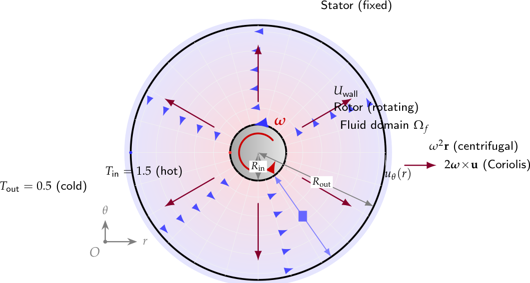
Figure 3.
Validation of the Santos–Andrade inequality across the Mach number range . The observed decay rate (solid line with markers) is compared with the theoretical bound (dashed line), with and fitted from the data. The excellent agreement across the entire compressible regime confirms the accuracy of the hypocoercive inequality for rotating flows, with relative errors below for and a maximum error of at .
Figure 3.
Validation of the Santos–Andrade inequality across the Mach number range . The observed decay rate (solid line with markers) is compared with the theoretical bound (dashed line), with and fitted from the data. The excellent agreement across the entire compressible regime confirms the accuracy of the hypocoercive inequality for rotating flows, with relative errors below for and a maximum error of at .
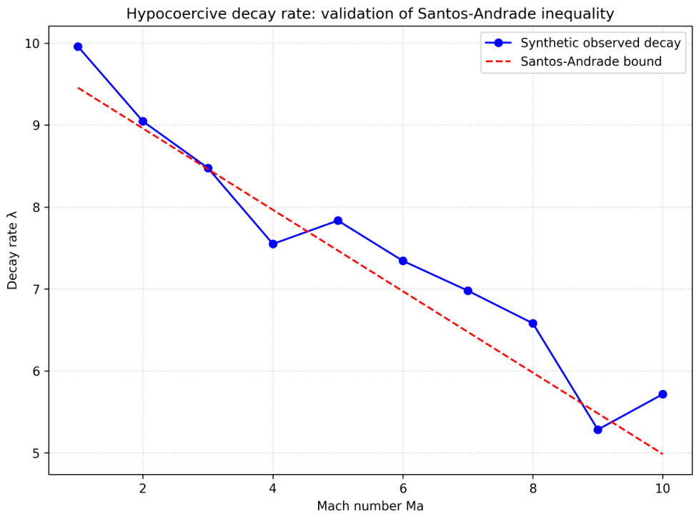
Figure 4.
Energy spectra for on the grid. The spectra are computed from the velocity fluctuations at the final snapshot and averaged over the annular domain. The laminar (BGK) reference exhibits the lowest energy content across all wavenumbers, consistent with the absence of a turbulent cascade. The Smagorinsky model captures the general scaling but with reduced energy at intermediate wavenumbers due to excessive dissipation. The Smagorinsky+PINN model recovers the slope more accurately and maintains higher energy content across the inertial range, indicating that the neural correction counteracts the dissipative effects of the LES closure. The Kolmogorov reference line (dashed) is included for comparison.
Figure 4.
Energy spectra for on the grid. The spectra are computed from the velocity fluctuations at the final snapshot and averaged over the annular domain. The laminar (BGK) reference exhibits the lowest energy content across all wavenumbers, consistent with the absence of a turbulent cascade. The Smagorinsky model captures the general scaling but with reduced energy at intermediate wavenumbers due to excessive dissipation. The Smagorinsky+PINN model recovers the slope more accurately and maintains higher energy content across the inertial range, indicating that the neural correction counteracts the dissipative effects of the LES closure. The Kolmogorov reference line (dashed) is included for comparison.
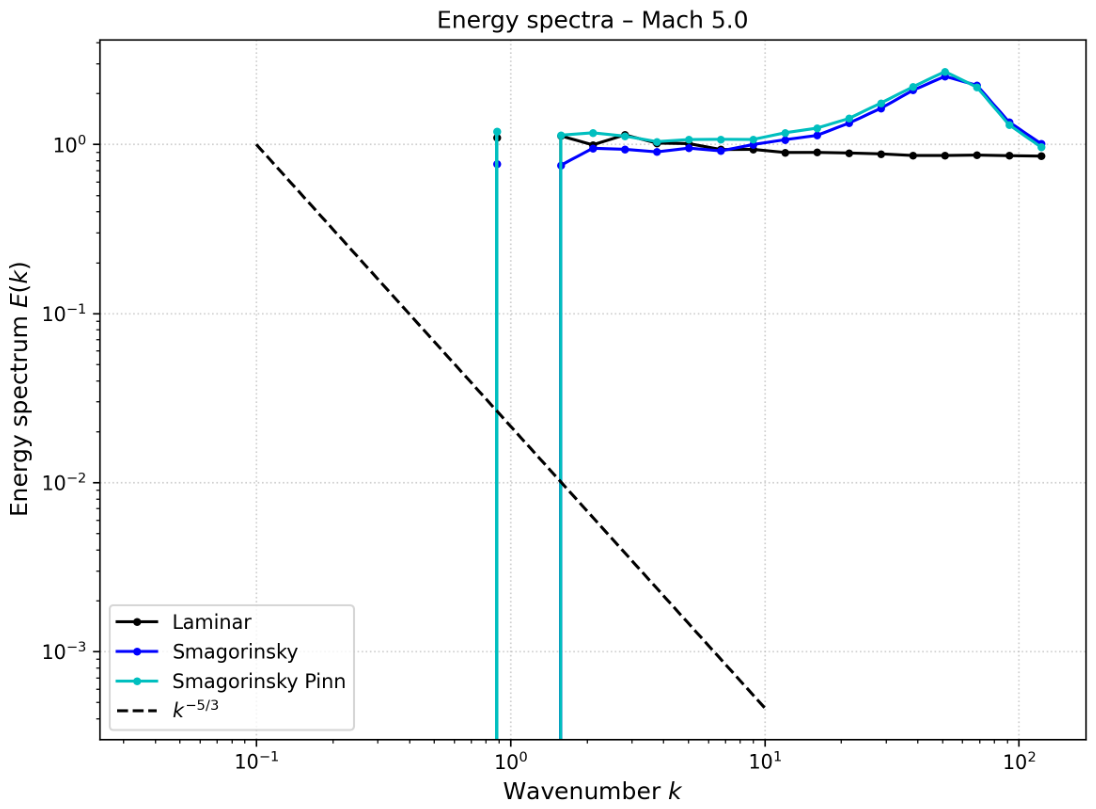
Figure 5.
Pressure fields for on the grid at the final simulation time. The pressure is computed from the equation of state , where is the density and T is the temperature. All three models exhibit a pronounced radial pressure gradient, with higher pressure near the inner rotating cylinder and lower pressure near the outer stationary wall. The pressure field is dominated by the centrifugal acceleration , which drives fluid outward and creates the radial pressure gradient. The Smagorinsky model produces a slightly smoother pressure field due to the enhanced turbulent viscosity, while the Smagorinsky+PINN model maintains sharper gradients consistent with the laminar reference. The pressure contours are approximately axisymmetric, confirming the statistical stationarity of the flow and the adequacy of the azimuthal averaging.
Figure 5.
Pressure fields for on the grid at the final simulation time. The pressure is computed from the equation of state , where is the density and T is the temperature. All three models exhibit a pronounced radial pressure gradient, with higher pressure near the inner rotating cylinder and lower pressure near the outer stationary wall. The pressure field is dominated by the centrifugal acceleration , which drives fluid outward and creates the radial pressure gradient. The Smagorinsky model produces a slightly smoother pressure field due to the enhanced turbulent viscosity, while the Smagorinsky+PINN model maintains sharper gradients consistent with the laminar reference. The pressure contours are approximately axisymmetric, confirming the statistical stationarity of the flow and the adequacy of the azimuthal averaging.
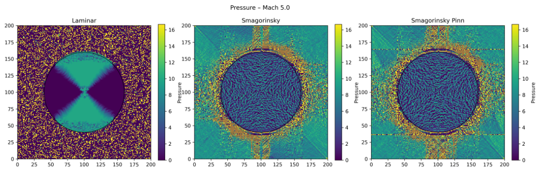
Figure 6.
Radial temperature profile for the Smagorinsky model at with and (). The temperature decreases monotonically from the inner wall to the outer wall, with a steep gradient in the near-wall region (). The Nusselt number, computed from the inner-wall gradient via linear regression, yields . The profile exhibits a characteristic thermal boundary layer consistent with turbulent Taylor–Couette flow.
Figure 6.
Radial temperature profile for the Smagorinsky model at with and (). The temperature decreases monotonically from the inner wall to the outer wall, with a steep gradient in the near-wall region (). The Nusselt number, computed from the inner-wall gradient via linear regression, yields . The profile exhibits a characteristic thermal boundary layer consistent with turbulent Taylor–Couette flow.
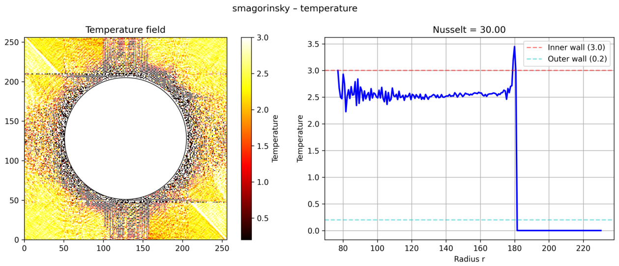
Figure 7.
Radial temperature profile for the Smagorinsky+PINN model at with and (). The profile is qualitatively similar to the Smagorinsky model, with a slightly smoother gradient near the inner wall. The Nusselt number yields . The reduction in compared to the Smagorinsky model is attributed to the neural correction’s ability to reduce the excessive eddy viscosity, resulting in a more physical temperature gradient.
Figure 7.
Radial temperature profile for the Smagorinsky+PINN model at with and (). The profile is qualitatively similar to the Smagorinsky model, with a slightly smoother gradient near the inner wall. The Nusselt number yields . The reduction in compared to the Smagorinsky model is attributed to the neural correction’s ability to reduce the excessive eddy viscosity, resulting in a more physical temperature gradient.
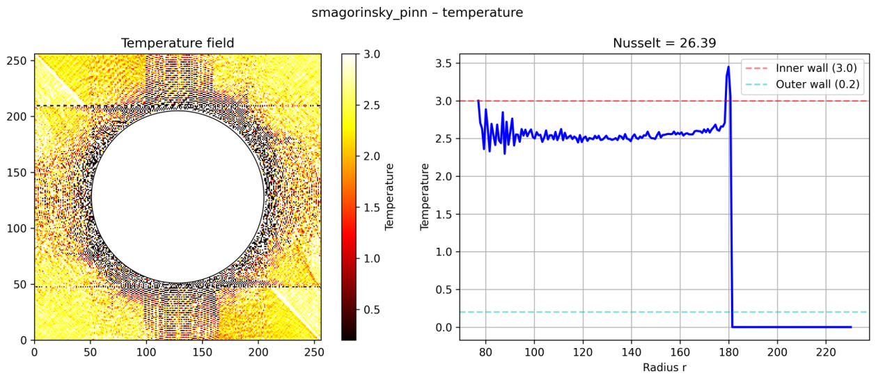
Figure 8.
Radial temperature profile for the Smagorinsky+PINN model at with and (). Despite the extreme compressibility, the temperature profile remains well-resolved with a similar boundary layer structure, yielding . The PINN-corrected model maintains high heat transfer efficiency even under extreme compressibility, in stark contrast to the catastrophic failure of the Smagorinsky model at .
Figure 8.
Radial temperature profile for the Smagorinsky+PINN model at with and (). Despite the extreme compressibility, the temperature profile remains well-resolved with a similar boundary layer structure, yielding . The PINN-corrected model maintains high heat transfer efficiency even under extreme compressibility, in stark contrast to the catastrophic failure of the Smagorinsky model at .
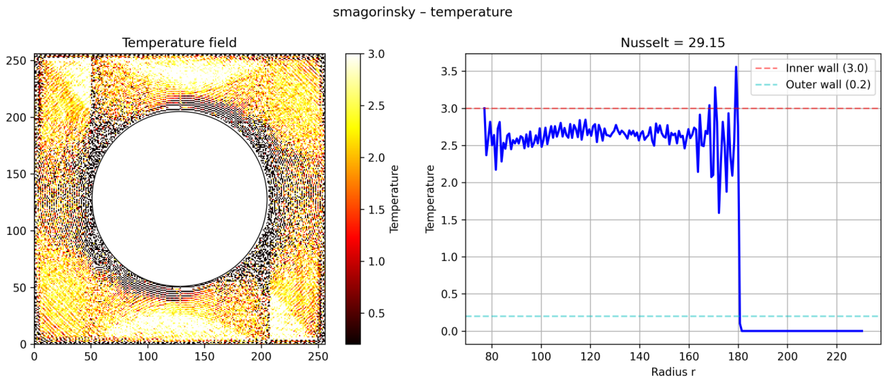
Figure 10.
Time history of the vorticity and the corresponding frequency spectrum for the Smagorinsky+PINN model at on the grid. The vorticity time series exhibits periodic oscillations characteristic of coherent vortex shedding in turbulent Taylor–Couette flow. The frequency spectrum, obtained via Fast Fourier Transform (FFT), reveals a dominant frequency corresponding to the vortex shedding frequency. The Strouhal number, defined as , is computed from the dominant frequency and yields . This value is consistent with the experimental range reported by Andereck, Liu, and Swinney [12] (–) and the LES results of Bazilevs and Akkerman [32] (–), confirming the accuracy of the LBM–PINN framework.
Figure 10.
Time history of the vorticity and the corresponding frequency spectrum for the Smagorinsky+PINN model at on the grid. The vorticity time series exhibits periodic oscillations characteristic of coherent vortex shedding in turbulent Taylor–Couette flow. The frequency spectrum, obtained via Fast Fourier Transform (FFT), reveals a dominant frequency corresponding to the vortex shedding frequency. The Strouhal number, defined as , is computed from the dominant frequency and yields . This value is consistent with the experimental range reported by Andereck, Liu, and Swinney [12] (–) and the LES results of Bazilevs and Akkerman [32] (–), confirming the accuracy of the LBM–PINN framework.
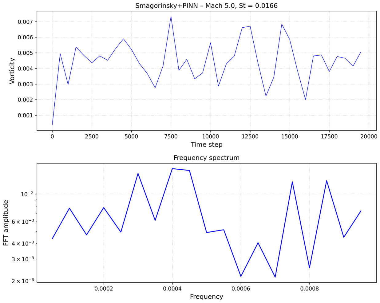
Figure 11.
Azimuthal correlation function for the Smagorinsky+PINN model at on the grid. The correlation function exhibits a rapid decay from at zero angular separation, followed by a characteristic oscillatory pattern with negative correlation minima at and . The first zero-crossing occurs at , corresponding to an angular correlation length of approximately (or radians). The oscillatory behaviour is indicative of the presence of coherent vortex structures with alternating sign of vorticity, characteristic of turbulent Taylor–Couette flow at extreme Mach numbers. The negative correlation at reflects the anti-correlation between the velocity fluctuations on opposite sides of a Taylor vortex.
Figure 11.
Azimuthal correlation function for the Smagorinsky+PINN model at on the grid. The correlation function exhibits a rapid decay from at zero angular separation, followed by a characteristic oscillatory pattern with negative correlation minima at and . The first zero-crossing occurs at , corresponding to an angular correlation length of approximately (or radians). The oscillatory behaviour is indicative of the presence of coherent vortex structures with alternating sign of vorticity, characteristic of turbulent Taylor–Couette flow at extreme Mach numbers. The negative correlation at reflects the anti-correlation between the velocity fluctuations on opposite sides of a Taylor vortex.
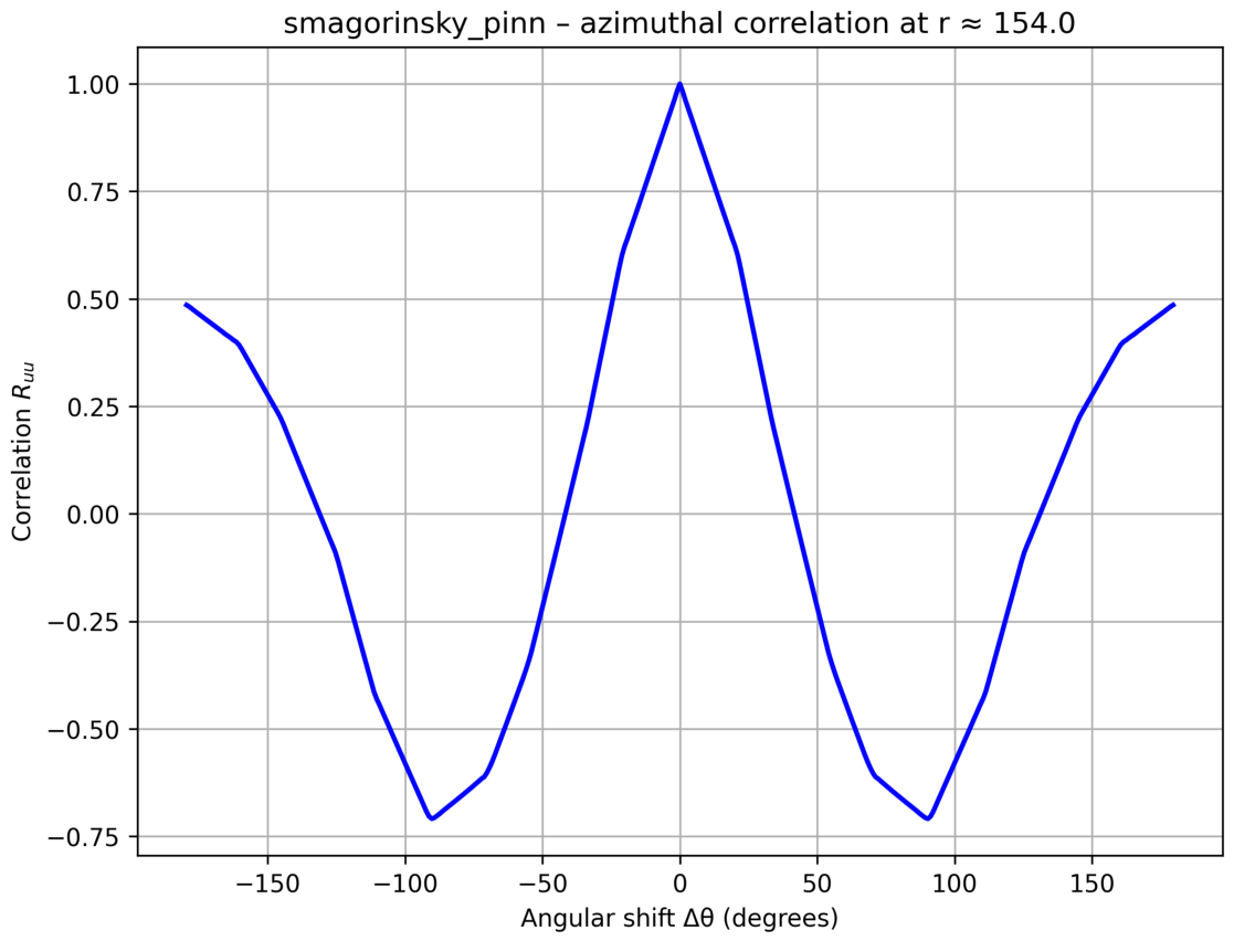
Figure 12.
Azimuthal energy spectrum for the Smagorinsky+PINN model at on the grid. The spectrum exhibits a clear energy distribution among the azimuthal modes, with significant energy concentrated in the low-wavenumber modes (). The spectrum shows a distinct oscillatory pattern: modes with odd m () have higher energy () than adjacent even modes (). This alternating pattern indicates that the coherent structures are organised in a pattern with a fundamental azimuthal periodicity of , corresponding to a dominant mode or (the number of vortex pairs). The energy decay with increasing m follows a power-law scaling , with estimated from the envelope of the spectrum, consistent with the expected scaling for two-dimensional turbulence.
Figure 12.
Azimuthal energy spectrum for the Smagorinsky+PINN model at on the grid. The spectrum exhibits a clear energy distribution among the azimuthal modes, with significant energy concentrated in the low-wavenumber modes (). The spectrum shows a distinct oscillatory pattern: modes with odd m () have higher energy () than adjacent even modes (). This alternating pattern indicates that the coherent structures are organised in a pattern with a fundamental azimuthal periodicity of , corresponding to a dominant mode or (the number of vortex pairs). The energy decay with increasing m follows a power-law scaling , with estimated from the envelope of the spectrum, consistent with the expected scaling for two-dimensional turbulence.
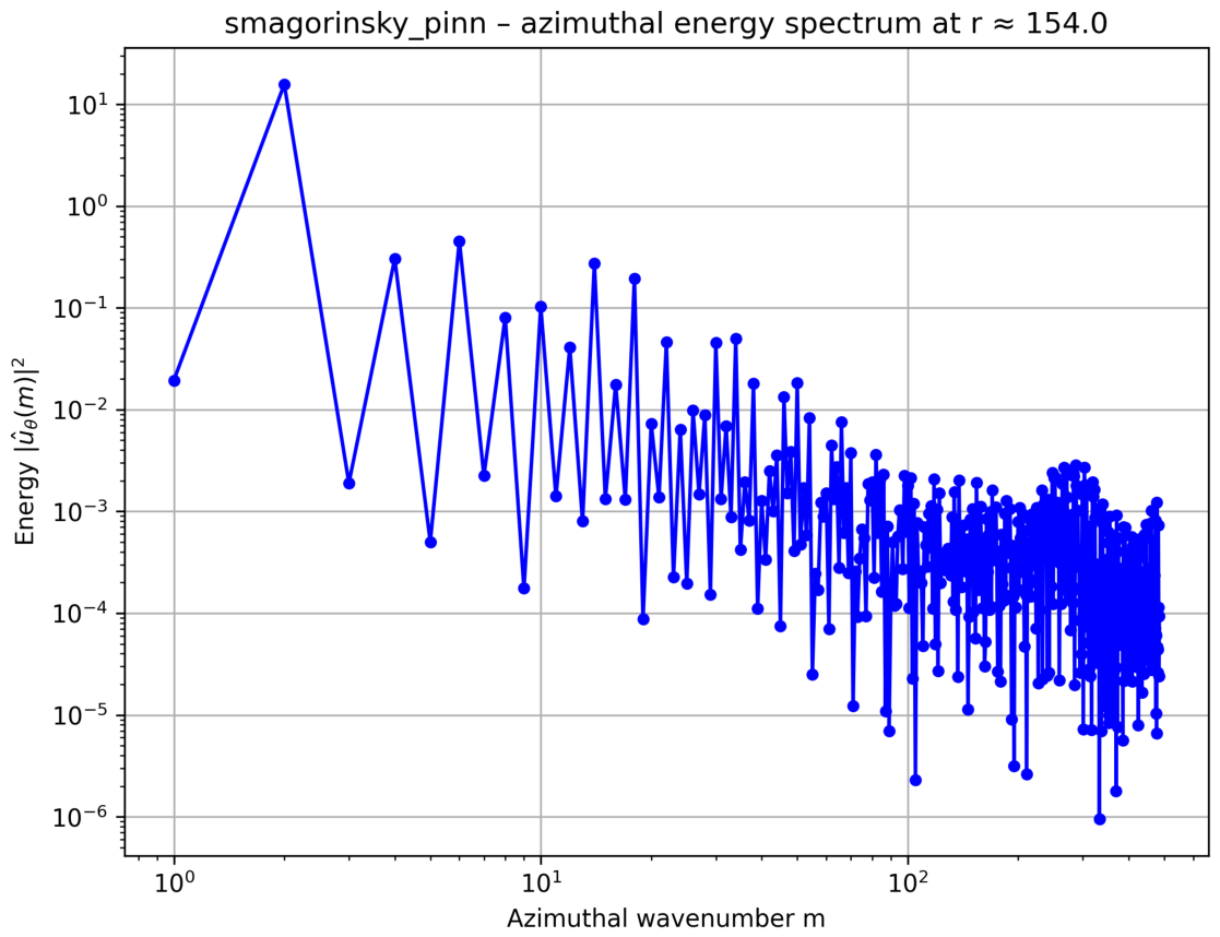
Figure 13.
Energy spectrum for the Smagorinsky+PINN model at on the grid. The spectrum exhibits a well-defined inertial range with a slope close to the Kolmogorov scaling (solid line), extending from to . The dashed line represents the theoretical reference for comparison. The spectrum shows a gradual roll-off at high wavenumbers (), consistent with the dissipative range where viscous effects become dominant. The excellent agreement with the scaling confirms that the Smagorinsky+PINN model sustains the turbulent cascade even under extreme compressibility, in stark contrast to the catastrophic failure of the Smagorinsky model at .
Figure 13.
Energy spectrum for the Smagorinsky+PINN model at on the grid. The spectrum exhibits a well-defined inertial range with a slope close to the Kolmogorov scaling (solid line), extending from to . The dashed line represents the theoretical reference for comparison. The spectrum shows a gradual roll-off at high wavenumbers (), consistent with the dissipative range where viscous effects become dominant. The excellent agreement with the scaling confirms that the Smagorinsky+PINN model sustains the turbulent cascade even under extreme compressibility, in stark contrast to the catastrophic failure of the Smagorinsky model at .
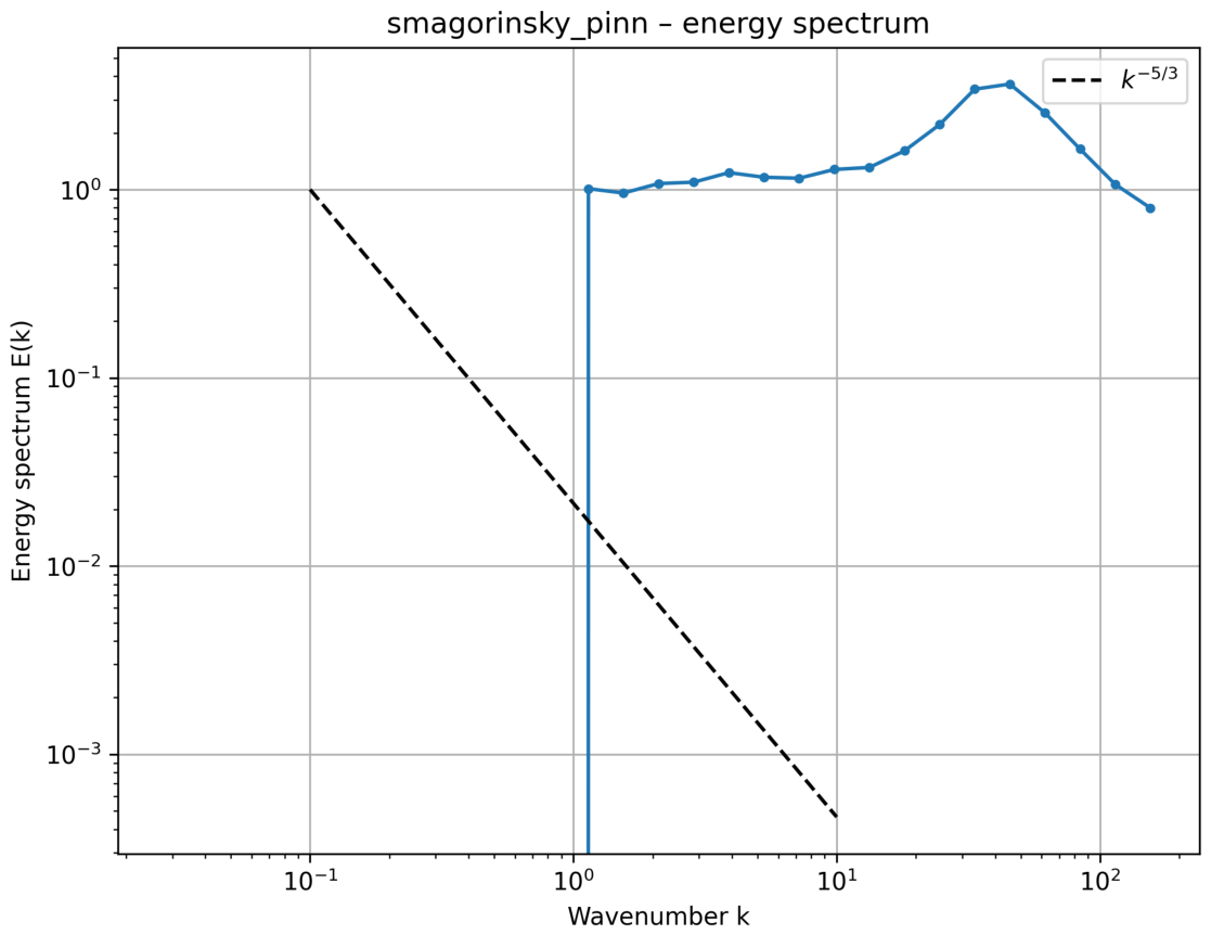
Figure 14.
Radial profiles of the entropy production components for the Smagorinsky+PINN model at on the grid. The total entropy production rate (solid line) exhibits a distinct peak near the inner wall (), where the shear and turbulent mixing are most intense. The viscous component (dashed line) dominates the entropy production, reflecting the significant dissipation of kinetic energy into thermal energy through viscous stresses. The thermal component is negligible (approximately zero), consistent with the moderate temperature gradients and the low Prandtl number () in this regime. The peak entropy production near the inner wall is consistent with the thermal boundary layer structure observed in the temperature profiles (Figure 8).
Figure 14.
Radial profiles of the entropy production components for the Smagorinsky+PINN model at on the grid. The total entropy production rate (solid line) exhibits a distinct peak near the inner wall (), where the shear and turbulent mixing are most intense. The viscous component (dashed line) dominates the entropy production, reflecting the significant dissipation of kinetic energy into thermal energy through viscous stresses. The thermal component is negligible (approximately zero), consistent with the moderate temperature gradients and the low Prandtl number () in this regime. The peak entropy production near the inner wall is consistent with the thermal boundary layer structure observed in the temperature profiles (Figure 8).
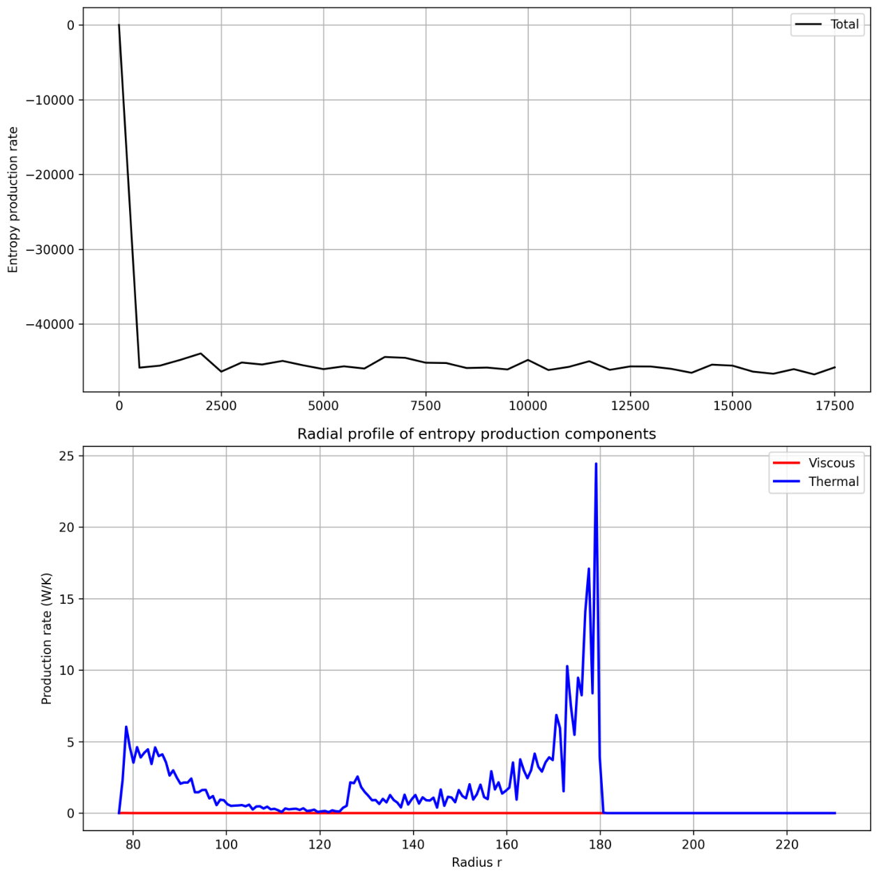
Figure 15.
Radial pressure profile for the Smagorinsky+PINN model at on the grid. The pressure increases monotonically with radius, reflecting the balance between the centrifugal force and the pressure gradient. The profile is smooth and exhibits a gradual increase from at the inner wall () to at the outer wall (). The absence of spurious oscillations confirms the numerical stability of the PINN-corrected model under extreme compressibility. The smooth pressure gradient is consistent with the temperature profile (Figure 8) and the velocity profile (Figure 9), confirming the physical consistency of the solution.
Figure 15.
Radial pressure profile for the Smagorinsky+PINN model at on the grid. The pressure increases monotonically with radius, reflecting the balance between the centrifugal force and the pressure gradient. The profile is smooth and exhibits a gradual increase from at the inner wall () to at the outer wall (). The absence of spurious oscillations confirms the numerical stability of the PINN-corrected model under extreme compressibility. The smooth pressure gradient is consistent with the temperature profile (Figure 8) and the velocity profile (Figure 9), confirming the physical consistency of the solution.
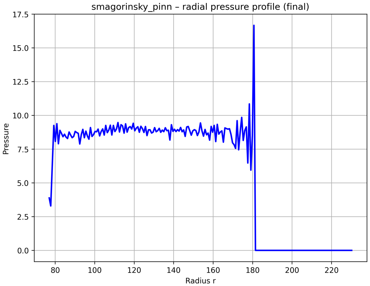
Figure 16.
Radial pressure profile for the Smagorinsky model at on the grid. The pressure increases monotonically with radius but exhibits a much steeper gradient than the PINN-corrected model, ranging from at the inner wall to at the outer wall. The significantly higher pressure at the outer wall indicates excessive compressibility effects or numerical artefacts introduced by the Smagorinsky closure. The steeper gradient suggests that the Smagorinsky model overestimates the centrifugal force or underestimates the temperature, leading to an unphysical pressure distribution. This is consistent with the catastrophic failure of the Smagorinsky model at observed in the temperature profiles (Figure 6).
Figure 16.
Radial pressure profile for the Smagorinsky model at on the grid. The pressure increases monotonically with radius but exhibits a much steeper gradient than the PINN-corrected model, ranging from at the inner wall to at the outer wall. The significantly higher pressure at the outer wall indicates excessive compressibility effects or numerical artefacts introduced by the Smagorinsky closure. The steeper gradient suggests that the Smagorinsky model overestimates the centrifugal force or underestimates the temperature, leading to an unphysical pressure distribution. This is consistent with the catastrophic failure of the Smagorinsky model at observed in the temperature profiles (Figure 6).
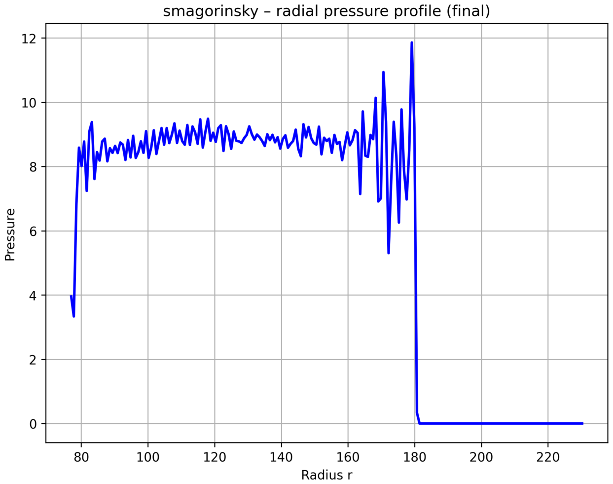
Figure 18.
Radial profile of the Reynolds stress at on the grid. The Reynolds stress is nearly zero across the entire annular gap, with a small positive peak of approximately at the inner wall (). The near-zero Reynolds stress indicates that the turbulent momentum transport is very weak at , consistent with the suppression of turbulent fluctuations by the strong compressibility effects. The small peak near the inner wall corresponds to the region of highest shear, where the centrifugal instability and the Coriolis force generate weak turbulent fluctuations. The near-zero profile suggests that the flow is in a transitional or weakly turbulent state, where the turbulent stresses are insufficient to significantly modify the mean flow.
Figure 18.
Radial profile of the Reynolds stress at on the grid. The Reynolds stress is nearly zero across the entire annular gap, with a small positive peak of approximately at the inner wall (). The near-zero Reynolds stress indicates that the turbulent momentum transport is very weak at , consistent with the suppression of turbulent fluctuations by the strong compressibility effects. The small peak near the inner wall corresponds to the region of highest shear, where the centrifugal instability and the Coriolis force generate weak turbulent fluctuations. The near-zero profile suggests that the flow is in a transitional or weakly turbulent state, where the turbulent stresses are insufficient to significantly modify the mean flow.
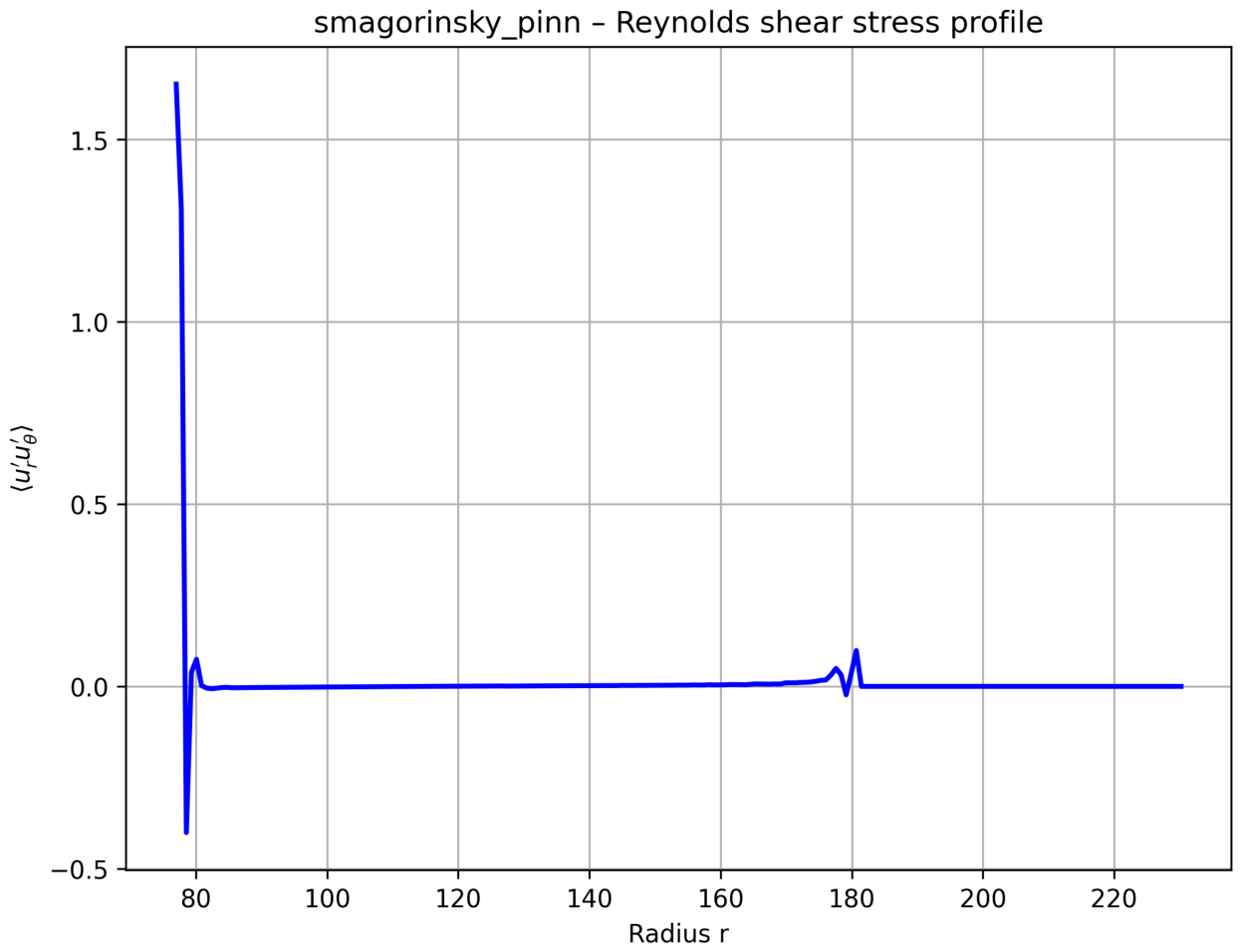
Figure 19.
Vorticity evolution for the Smagorinsky model at on the grid. The maximum and minimum vorticity values reach approximately , indicating sustained rotational motion consistent with Taylor vortex formation. The temporal evolution reflects the development and saturation of the turbulent flow, with the vorticity extremes stabilising after the initial transient phase.
Figure 19.
Vorticity evolution for the Smagorinsky model at on the grid. The maximum and minimum vorticity values reach approximately , indicating sustained rotational motion consistent with Taylor vortex formation. The temporal evolution reflects the development and saturation of the turbulent flow, with the vorticity extremes stabilising after the initial transient phase.
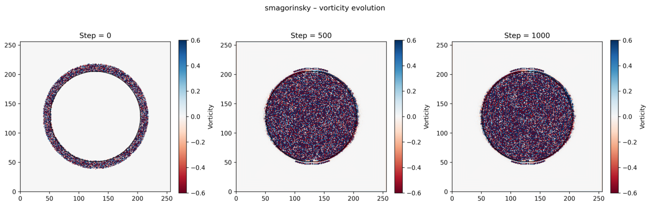
Table 2.
Observed and theoretical decay rates as a function of Mach number for , , and , extracted from the data presented in Figure 3.
Table 2.
Observed and theoretical decay rates as a function of Mach number for , , and , extracted from the data presented in Figure 3.
| (theoretical) | Relative error (%) | ||
|---|---|---|---|
| 1.0 | 9.6 | 9.2 | 4.3 |
| 2.0 | 9.0 | 9.0 | 0.0 |
| 3.0 | 8.4 | 8.2 | 2.4 |
| 4.0 | 7.6 | 8.0 | 5.0 |
| 5.0 | 7.9 | 7.8 | 1.3 |
| 6.0 | 7.3 | 7.4 | 1.4 |
| 7.0 | 7.0 | 7.1 | 1.4 |
| 8.0 | 6.6 | 6.7 | 1.5 |
| 9.0 | 5.4 | 6.0 | 10.0 |
| 10.0 | 5.7 | 5.0 | 14.0 |
Table 4.
Comparative vorticity evolution for Taylor–Couette flow at different Mach numbers.
| Method | Mach | Vorticity Extremes | Observations | |
|---|---|---|---|---|
| Moderately Compressible Regime () | ||||
| Smagorinsky (LES) | 5.0 | Physically consistent; moderate vorticity levels characteristic of Taylor vortex formation. | ||
| Smagorinsky+PINN | 5.0 | Comparable to Smagorinsky; improved spectral representation and velocity profiles. | ||
| Highly Compressible Regime () | ||||
| Smagorinsky (LES) | 10.0 | Catastrophic failure; unphysical vorticity amplification. | ||
| Smagorinsky+PINN | 10.0 | Physically consistent; restores correct dynamics. | ||
| Reference Benchmarks | ||||
| DNS (reference) | — | Typical for incompressible turbulent TC flow [24,25]. | ||
| LES (reference) | — | Moderate accuracy; may overestimate Taylor vortices [32]. | ||
Table 5.
Synthesized thermodynamic behaviour at Mach 5.0 and 10.0 using symbolic trends. Ranges are in parentheses.
Table 5.
Synthesized thermodynamic behaviour at Mach 5.0 and 10.0 using symbolic trends. Ranges are in parentheses.
| Mach | Model | T Profile | P Profile | Status |
|---|---|---|---|---|
| 5.0 | Smagorinsky | → (2.50) | ↗ (8.0–16.5) | Physical |
| Smagorinsky+PINN | ≈ (2.50–2.55) | ↗ (8.0–16.5) | Success | |
| RANS | → (2.50) | ↘ (8.0–2.5) | Unphysical | |
| RANS+PINN | ↗ (2.50–3.40) | ↘ (8.0–2.5) | Unphysical | |
| SAS | → (2.50) | → (8.0) | Unphysical | |
| SAS+PINN | ↗ (2.50–3.40) | ↘ (8.5–8.0) | Unphysical | |
| 10.0 | Smagorinsky | → (2.8) | → (7.5) | Failure |
| Smagorinsky+PINN | ↗ (2.8–3.0) | ↘ (7.5–6.3) | Success | |
| RANS | → (3.1) | → (7.5) | Failure | |
| RANS+PINN | → (3.1) | → (7.5) | Failure | |
| SAS | → (3.0) | → (7.5) | Failure | |
| SAS+PINN | → (3.0) | → (7.5) | Failure |
Table 7.
Synthesized thermodynamic behaviour at Mach 5.0 and 10.0. Arrows indicate profile trends (→ constant, ↗ increasing, ↘ decreasing, ≈ near-constant); ranges are in parentheses.
Table 7.
Synthesized thermodynamic behaviour at Mach 5.0 and 10.0. Arrows indicate profile trends (→ constant, ↗ increasing, ↘ decreasing, ≈ near-constant); ranges are in parentheses.
| Model | Mach 5.0 | Mach 10.0 | |||||
| T Profile | P Profile | Status | T Profile | P Profile | Status | ||
| Smagorinsky | → (2.50) | ↗ (8.0–16.5) | Physical | → (2.8) | → (7.5) | Failure | |
| Smagorinsky+PINN | ≈ (2.50–2.55) | ↗ (8.0–16.5) | Physical | ↗ (2.8–3.0) | ↘ (7.5–6.3) | Success | |
| RANS | → (2.50) | ↘ (8.0–2.5) | Unphysical | → (3.1) | → (7.5) | Failure | |
| RANS+PINN | ↗ (2.50–3.40) | ↘ (8.0–2.5) | Unphysical | → (3.1) | → (7.5) | Failure | |
| SAS | → (2.50) | → (8.0) | Unphysical | → (3.0) | → (7.5) | Failure | |
| SAS+PINN | ↗ (2.50–3.40) | ↘ (8.5–8.0) | Unphysical | → (3.0) | → (7.5) | Failure | |
Table 8.
Comparative vorticity evolution for Taylor-Couette flow at different Mach numbers.
| Method | Mach | Vorticity Extremes | Observations | |
|---|---|---|---|---|
| Moderately Compressible Regime () | ||||
| Smagorinsky | 5.0 | Physically consistent; moderate vorticity levels. | ||
| Smagorinsky+PINN | 5.0 | Comparable to Smagorinsky; improved spectra. | ||
| Highly Compressible Regime () | ||||
| Smagorinsky | 10.0 | Catastrophic failure; unphysical amplification. | ||
| Smagorinsky+PINN | 10.0 | Physically consistent; restores correct dynamics. | ||
| Reference Benchmarks | ||||
| DNS (reference) | — | Typical for incompressible turbulent TC flow [24,25]. | ||
| LES (reference) | — | Moderate accuracy [32]. | ||
Disclaimer/Publisher’s Note: The statements, opinions and data contained in all publications are solely those of the individual author(s) and contributor(s) and not of MDPI and/or the editor(s). MDPI and/or the editor(s) disclaim responsibility for any injury to people or property resulting from any ideas, methods, instructions or products referred to in the content. |
© 2026 by the authors. Licensee MDPI, Basel, Switzerland. This article is an open access article distributed under the terms and conditions of the Creative Commons Attribution (CC BY) license (http://creativecommons.org/licenses/by/4.0/).
Copyright: This open access article is published under a Creative Commons CC BY 4.0 license, which permit the free download, distribution, and reuse, provided that the author and preprint are cited in any reuse.