

Submitted:
13 August 2026
Posted:
14 August 2026
You are already at the latest version
Abstract
Marine cage aquaculture contributes to nutrient enrichment of the surrounding waters, with ammonium (NH4+) being the predominant ionized form of inorganic nitrogen (N) released. Elevated NH4+ concentrations in marine waters may promote excessive phytoplankton growth, which may subsequently affect the ecological status of the surrounding ecosystem under certain environmental conditions. This study aims to investigate the potential of Sentinel-2 MSI imagery for estimating NH4+ in an oligotrophic semi-enclosed cove where marine cage aquaculture operates. Firstly, the relationship between in situ NH4+ and chlorophyll a (chl a) measurements was evaluated, both on a seasonal basis and across all seasons, to determine whether chl a could serve as a proxy for NH4+ estimation. Given the weak correlation observed, the feasibility of direct NH4+ retrieval was further evaluated. A band-selection procedure was applied to retain Sentinel-2 MSI spectral bands with the highest correlation with NH4+ while minimizing multicollinearity arises from spectral “overlap” among bands. To evaluate the effectiveness of the proposed band-selection procedure in improving the generalization ability of three machine learning (ML) models, the complete set of Sentinel-2 MSI spectral bands at 10 and 20 m spatial resolutions was also used. The obtained RMSE and MAE values (0.29 and 0.22 μM, respectively) for the Random Forest–Bayesian Optimization with Tree-structured Parzen Estimator (RF-BO-TPE) and Support Vector Regression–Bayesian Optimization with Tree-structured Parzen Estimator (SVR-BO-TPE) models in the testing dataset, using the selected spectral bands (B03, B04, B05 and B08), indicated reasonable agreement with the actual NH₄⁺ concentrations (Range: 0.00-1.46 μΜ, SD = ±0.20 μM). Furthermore, the observed robustness against overfitting (ΔR² = 0.07, ORRMSE = 1.10–1.11, and ORMAE = 1.01–1.02) suggests that the developed models could provide useful NH₄⁺ estimates. These findings highlight the potential of Sentinel-2 MSI for NH₄⁺ estimation in oligotrophic coastal waters affected by cage aquaculture.
Keywords:
remote sensing
; aquaculture
; water quality
; nutrients
; coastal
; oligotrophic
; band-selection
; multicollinearity
; machine learning
; overfitting
1. Introduction
Intensive fish farming takes place in floating sea cages which are placed near the surface of the water column, particularly in coastal waters. It is characterized as an open cultivation system, where water passes freely through the cages, and interacts with the marine environment by producing effluents that are released directly into water. The metabolic processes of cultivated fish and the uneaten feed tend to result in nutrient release [1]. Although marine cage aquaculture contributes only 1% to total nutrient enrichment in coastal water bodies compared with other anthropogenic activities [2], it remains a relevant source of nutrient loading particularly in semi-enclosed areas.
Ammonium (NH4+) is the main ionized nitrogen (N) form produced by fish farming [3] and it is the most preferred N source for phytoplankton growth [4]. Therefore, systematic monitoring of NH4+ in areas where fish farming takes place is essential, as increased NH4+ flux may stimulate excessive phytoplankton growth, which, under certain environmental conditions, could affect the ecological status of the surrounding ecosystem. In aquaculture environments, the estimation of water quality parameters, including NH4+, is particularly based on field measurements, sampling and laboratory analysis. Although these methods provide extremely accurate results, they are costly, time-consuming and they are only able to provide point estimations. Recently, remote sensing has been applied as an alternative approach for estimating water quality parameters (WQPs) in both coastal [5,6,7,8] and inland [9,10,11,12] water bodies, associated with aquaculture operations, providing cost-effective, large-scale datasets with high temporal frequency [13].
Unlike optically active constituents (OACs) of water, the estimation of NH4+ using remote sensing remains challenging because NH4+ lacks a direct optical signature and does not significantly influence the absorption and scattering properties of water. In general, the retrieval of nutrients from remotely sensed data has relied on empirical, machine learning (ML) and deep learning (DL) approaches [14], with model development primarily exploiting the indirect relationships between non-OACs and OACs, such as chl a, total suspended matter (TSM) and colored dissolved organic matter (CDOM) [15]. However, these relationships may vary across water bodies due to differences in spatial and temporal characteristics, as well as trophic conditions, which regulate OAC abundance and consequently affect optical properties and the retrieval of non-OACs [14].
An alternative approach involves the direct estimation of non-OACs from remotely sensed data without prior retrieval of OACs [16,17]. This strategy relies increasingly on ML and DL approaches capable of capturing complex non-linear relationships between spectral bands and non-OACs of water [14,17]. Comparative studies have shown that ML models may demonstrate better generalization performance than DL models under conditions of limited data availability, as they are generally less prone to overfitting when trained on small datasets [14]. Overfitting is one of the major challenges in ML because models that perform well on training datasets may fail to generalize to unseen data [18].
The majority of remote sensing-based studies on nutrient estimation has focused on eutrophic or hypertrophic water bodies influenced by agricultural, industrial, and/or urban wastewater runoff, while the effect of seasonal variability has received limited attention [14]. This study aims to investigate the potential of multispectral Sentinel-2 MSI imagery for estimating NH4+ in an oligotrophic semi-enclosed cove where a marine cage aquaculture operates. Firstly, the relationship between in situ NH4+ concentrations and chl a was assessed, both on a seasonal basis and across the entire dataset, to determine whether chl a could serve as a reliable proxy for NH4+ estimation. Given the weak correlation observed between NH4+ and chl a, the feasibility of direct NH4+ retrieval was further evaluated. A band-selection procedure was applied to retain Sentinel-2 MSI spectral bands with the highest correlation with NH4+ while minimizing multicollinearity arises from spectral “overlap” among bands. The Extreme Gradient Boosting—Particle Swarm Optimization (XGBoost-PSO), Random Forest—Bayesian Optimization with Tree-structured Parzen Estimator (RF-BO-TPE) and Support Vector Regression—Bayesian Optimization with Tree-structured Parzen Estimator (SVR-BO-TPE) models were developed for NH4+ estimation. Models’ generalization ability was subsequently assessed using the difference in the coefficient of determination (ΔR2) and overfitting ratios derived from RMSE and MAE (ORRMSE and ORMAE).
2. Materials and Methods
2.1. Study Area
The marine cage aquaculture site is located in the southeastern part of Pagasitikos Gulf (Eastern Mediterranean, Greece), within a semi-enclosed cove (39◦07′38” N, 23◦09′ 17” E). It comprises 18 polyethylene cages, including 12 cages with dimensions of 7.5 × 15 × 8 m and 6 cages with dimensions of 15 × 15 × 10 m (length × width × depth). Sea bream (Sparus aurata) and sea bass (Dicentrarchus labrax) are intensively cultivated, using pelleted and extruded diets. The average annual standing stocks is 130 tonnes, while the final stocking density is calculated at 8 kg/m3. The feed conversion ratio (FCR), which represents the feed requirement per kilogram of body weight gain, is 1.7. The recorded circulation patterns indicate that the cove is characterized by weak currents throughout the year [19]. The prevailing circulation is directed from the northwest toward the inner part of the cove, where the fish cages are located, before exiting toward the southwest, with an average current speed of 3.5 cm s-1 [20]. The study area does not exhibit significant anthropogenic influence, with no identifiable pollution sources detected, while the surrounding landscape is dominated by olive cultivation and shrub vegetation. Consistent with the Eastern Mediterranean pattern of primary production [21], the cove represents an oligotrophic, phosphorus (P)-limited system, where low P availability constrains phytoplankton growth and maintains chl a at low levels [19].
2.2. In Situ Measurements
The sampling was carried out over six seasons, between summer 2021 and spring 2024, using a predefined sampling grid [20]. A total of 152 surface (0m) water samples were collected by means of a 1.4 ℓ Lymnos bottle and placed in 500 ml plastic vials for NH4+ estimation. Mercury chloride (2 ml of HgCl2 0.1 M per 500 ml sample) was added to inhibit any biological activity. Then, samples were stored at -20 °C until the analysis took place. Chemical analysis of the NH4+ was based on the methodology developed by [22], using a spectrophotometer (SHIMADZU UV-1800). Simultaneous surface in situ measurements of sea surface temperature (SST), sea surface salinity (SSS), pH and chl a were also obtained using a conductivity-temperature-depth (CTD) instrument (SEABIRD-19plus). All sampling procedures and measurements were carried out during the feeding period, between 09:00 and 14:00.
2.3. Statistical Analysis of In Situ Measurements
Descriptive statistics (minimum, maximum, mean ± standard deviation and median) were calculated for each WQP across seasons [23]. The Shapiro-Wilk (W) test [24] was conducted to evaluate whether the WQPs are normally distributed. The W test is widely used for assessing normality across a wide range of distributions and sample sizes [25,26] by evaluating the correlation between the ordered sample observations and the expected order statistics from a theoretical normal distribution. When this correlation is weak, the resulting p value falls below 0.05, indicating a deviation from normality [24]. The W test is given by Equation (1) [25]:
where is the order statistic, is the sample mean, and are the expected values of the order statistics of independent and identically distributed random variables samples from the standard normal distribution and V is the covariance matrix of those order statistics. Along with the W test, histograms [23] were also created to examine the normality assumption of WQPs. The strength of association between each pair of the five WQPs was assessed using Spearman’s rank correlation coefficient (ρ). The ρ is a standardized, non-parametric statistic that can be applied when the assumption of normality is violated. It works by fist ranking the data and then applying the Pearson’s correlation coefficient (rs) (Equation (2)) [27],
where are the ranked versions of variables x and y, cov is the covariance between ranks and σ is the standard deviation of ranks. The Spearman’s rank correlation coefficient (ρ) ranges between -1 ≤ ρ ≤ +1 and a high absolute value indicates that there is a monotonic, but not necessarily linear correlation between two variables [28]. In the present study, the correlation between WQPs was calculated both on a seasonal basis and across all seasons. In addition, scatterplots [23] were created to illustrate the relationship between each pair of variables.
The Krustal-Wallis (H) test [29] was selected to assess whether the values of each WQP differed significantly among seasons. It is a non-parametric, rank test, applied when the assumption of normality is not met, and it is used to compare three or more independent groups in terms of their distributions. The null-hypothesis of the H test assumes that the distribution of the test variable is identical across the diverse groups. Rejecting the null hypothesis means that the distributions differ in their central tendency, spread and/or variability [23]. The H test is given by the Equation (3) [29],
where N is the total number of observations, k is the number of groups, is the number of observations in group i and is the sum of ranks in group i.
The Dunn’s post hoc test [30] was applied to identify the specific seasons between which statistically significant differences were detected for each WQP. This non-parametric pairwise multiple comparison procedure was performed after rejecting the null hypothesis of the Krustal-Wallis. The Dunn test evaluates differences between groups based on ranked observations rather than the original data values, making appropriate for datasets that do not satisfy the assumption of normality. All observations were ranked jointly across groups and the mean rank for each group was calculated by Equation (4) [31],
where is the mean rank of the ith group, is the sum of ranks assigned to observations within that group and is the number of observations in the ith group. For each pairwise comparison between two groups (e.g., A and B), the Dunn test statistics is calculated as (Equation (5)),
where is the standardized test statistic, and are the mean ranks of groups A and B, respectively and is the standard error of the difference between mean ranks, calculated as (Equation (6)),
where N represents the total number of observations across all groups, and are the sample sizes of the two compared groups and represents the number of observations associated with the tth tied rank. The second term inside the brackets represents the correction for tied ranks. When no tied observations occur, this correction term becomes zero. In order to evaluate WQPs distribution across different seasons, boxplots [23]were also created.
2.4. Satellite Data
Atmospherically corrected Multispectral Sentinel-2 (MSI) Level-2A (L2A) images were selected close to the sampling dates, under free cloud conditions, and provided through the Copernicus Data Space Ecosystem (CDSE) [32]. Based on the coordinates received during sampling, pixel-to-point matching was performed, and surface reflectance values were extracted using SNAP (v.13.0). A factor of 1/10.000 was applied to L2A digital numbers (DN) to retrieve physical surface reflectance values [33]. The 60 m resolution Level-2A spectral bands were excluded due to their coarse spatial resolution, since mixed pixels containing water and non-water features (e.g., land-water interfaces and floating fish cages) may reduce the reliability of spectral information used for NH4+ modelling.
2.5. Spectral Band-Selection
A band-selection procedure was applied to retain Sentinel-2 MSI spectral bands with the highest correlation with NH4+ while minimizing multicollinearity arising from spectral “overlap” among bands. Multicollinearity refers to a data issue that occurs when two or more predictor variables, within a dataset, are highly correlated [23]. In statistical analysis and ML, strong relationships between input variables may reduce the reliability and precision of the estimates, leading to overfitting and poor generalization to new, unseen data [34]. The procedure combined Spearman correlation-based ranking and variance inflation factor (VIF)-based spectral band selection. VIF is the most widely used indicator of multicollinearity and is obtained through a separate regression procedure [23]. VIF values ≥ 10 and 5 < VIF ≤ 10 indicate severe and moderate multicollinearity, respectively [35].
Spectral bands were first ranked based on their Spearman correlation coefficients with NH4+ because the Shapiro-Wilk test indicated that the data were not normally distributed (p < 0.05). The band-selection procedure then iteratively evaluated each band, beginning with the highest-ranked one. At each iteration, the “candidate” band was temporarily added to the subset of previously selected bands and multicollinearity was assessed using the VIF. The “candidate” band was retained only when the maximum VIF of the resulting subset remained below the predefined threshold (VIF ≤ 5), otherwise, it was discarded. This procedure was repeated until all spectral bands were evaluated. To assess the effectiveness of the proposed band-selection procedure, the complete set of Sentinel-2 MSI spectral bands, at 10 m and 20 m spatial resolutions, was also used for NH4+ estimation.
2.6. Machine Learning (ML) Models
The XGBoost, RF and SVR were developed for NH4+ estimation. These models were selected because they demonstrate better predictive performance compared to other regression-based ML models and neural networks (NN) architectures under limited data availability [14]. The XGBoost was implemented in Python using the XGBoost library, whereas RF and SVR were implemented using the scikit-learn library.
XGBoost is an ensemble ML model designed for improved speed and performance, which use boosting and gradient descent techniques to combine multiple decision trees. In regression tasks, each new tree is built sequentially in a way that focuses on correcting the errors of the previous trees, influenced by the residuals of the earlier ones. The final prediction is obtained by aggregating the outputs of all trees [36]. RF is an ensemble ML model that applies the bagging strategy to combine multiple decision trees. In regression tasks, individual trees are trained on randomly selected subsets of the training data. The final output is computed by averaging the output of all trees, leading to improved generalization and reduced variance. SVR is a supervised ML model designed for regression tasks. The algorithm implicitly maps the input data into a higher-dimensional feature space using kernel functions, enabling the modeling of complex nonlinear relationships between input variables and the target [36,37].
Hyperparameter optimization (HPO) of the XGBoost model was performed using Particle Swarm Optimization (PSO) implemented through PySwarms library in Python, whereas the RF and SVR models were optimized using Bayesian optimization based on the Tree-structured Parzen Estimator (BO-TPE) algorithm within the Optuna framework. The hyperparameters considered for the XGBoost model included n_estimators, max_depth, learning_rate, subsample and colsample_bytree, while those considered for the RF model included n_estimators, max_depth, criterion, min_samples_split, min_samples_leaf and max_features [36]. For the SVR model, the radial basis function (RBF) was chosen as the kernel function, following previous studies that have successfully applied this kernel for similar modelling tasks [14]. Additionally, the RBF was selected due to its ability to capture complex nonlinear relationships and its relatively simple model configuration [36,37]. Therefore, the hyperparameters considered for the SVR model included C, gamma and epsilon. In all models, the optimization process was performed by minimizing the 5-fold cross-validation mean squared error (CV-MSE) [36].
2.7. Assessment of ML Models’ Generalization Ability
The dataset was randomly split into two subsets at an 8:2 ratio, with 80% of the samples (n = 121) used for training the ML models and the remaining 20% (n = 31) used for testing. The same train-test split was used for all developed models to ensure a fair and consistent evaluation of model performance. Three commonly used performance evaluation metrics, including the coefficient of determination (R2), root mean squared error (RMSE) and mean absolute error (MAE) were calculated based on the training subset. The R2 provides the proportion of variance explained by the model and is described by Equation (7):
where n is the number of samples, and represent the actual and predicted value for sample i, respectively, while denotes the average of actual values. The R2 is typically ranges between 0 and 1, whereas higher values indicate a better fit of the model. The RMSE (Equation (8)) and MAE (Equation (9)) quantify the magnitude of the models’ predictive errors and are expressed in the same units as the target variables. Models’ performance improves as the values of the error-based metrics decrease [18,38].
The developed models were tested on the unseen dataset using the same metrics. Models’ generalization ability was quantified using the difference between the R2 values obtained from the training and testing datasets (ΔR2) [39] and the overfitting ratios (ORRMSE and ORMAE) which are given by Equations 10 and 11:
where RMSEtest, MAEtest, RMSEtrain and MAEtrain are the RMSE and MAE calculated during testing and training process of ML models, respectively. ΔR2 values close to 0, as well as RMSE and MAE ratios close to 1, indicate the absence of overfitting and, consequently, good generalization ability [38,40].
3. Results
3.1. In Situ Measurements
Table 1 shows the minimum, maximum and mean ± standard deviation (SD) of in situ SST, SSS, pH, chl a and NH4+ measurements across different seasons. To assess the distribution of each WQP, histograms were used alongside the Shapiro-Wilk test, both on a seasonal basis and across all seasons. The histograms initially indicated deviations from the normal distribution, which were subsequently confirmed by the Shapiro-Wilk test (p < 0.05), resulting in the rejection of the null hypothesis of normality (Figure 1a–e).
The non-parametric Spearman’s rank correlation coefficient (ρ) was used to evaluate the pairwise correlation among WQPs, both seasonally and across the entire dataset. For individual seasons, the ρ values ranged from -0.26 to 0.18, indicating a weak correlation between chl a and NH4+, whereas a weak negative correlation (ρ = -0.41) was observed when considering all seasons together. Scatterplots were also used to illustrate how the two variables are related to each other. In general, the data points showed a random, non-uniform, scattered pattern, without a specific direction, indicating the absence of relationship between them (Figure 1a–e).
The non-parametric Krustal-Wallis test was used to assess whether the values of each WQP differed significantly among seasons. The null-hypothesis of Krustal-Wallis test was rejected (p < 0.05), indicating significant seasonal differences for all WQPs. The Dunn’s test was then conducted to identify the specific seasons between, which statistically significant differences were detected. The results of the pairwise multiple comparisons are given in Table 2. The boxplots (Figure 2) represent WQPs distribution across different seasons.
3.2. Spectral Band-Selection
In the present study, the band-selection procedure was initiated with 10 Sentinel-2 MSI spectral bands (B02, B03, B04, B05, B06, B07, B08, B8A, B11 and B12). Firstly, the VIF was used to assess potential multicollinearity among the spectral bands. For B07, B8A, B08, B12, B06, B11 and B05 the VIF values exceeded 10, indicating severe multicollinearity, while moderate collinearity (5 < VIF ≤ 10) was observed for B03 and B02 (Figure 3). The findings highlighted the need to address multicollinearity before incorporating spectral bands into the ML models. Then, spectral bands were ranked according to their Spearman correlation with NH4+ concentrations (Figure 4) and iteratively selected under a VIF ≤ 5 to address multicollinearity. Figure 5 presents the reduced dataset of spectral bands identified through band-selection procedure (B03, B04, B05 and B08) and their relative importance in NH4+ estimation.
3.3. Assessment of ML Models’ Generalization Ability
The spectral bands (B03, B04, B05 and B08) selected, through band-selection procedure, were used to develop the XGBoost (PSO), RF (BO-TPE) and SVR (BO-TPE) models. To evaluate the effect of band selection, the models were also developed using the complete set of Sentinel-2 MSI spectral bands, at 10 m and 20 m spatial resolutions. Table 3 presents the generalization ability of the ML models using the difference in the coefficient of determination (ΔR2) and overfitting ratios (ORRMSE and ORMAE), calculating using the R2, RMSE and MAE values obtained during the training and testing processes, respectively. The XGBoost (PSO) model exhibited high overfitting when using either the complete set of spectral bands or the reduced one. The ΔR2 values (0.53 and 0.45, respectively) were greater than 0, while ORRMSE (1.80) and ORMAE (1.77) exceeded 1, indicating lower performance and higher prediction errors in the test dataset compared with the training dataset. A similar overfitting pattern was also observed for the RF (BO-TPE) model developed using the complete set of spectral bands. Only the SVR (BO-TPE) model showed moderate overfitting when trained using the complete set of spectral bands. Both the RF (BO-TPE) and SVR (BO-TPE) models demonstrated good generalization ability when developed using only the B03, B04, B05 and B08 bands (ΔR2 = 0.07, ORRMSE = 1.11, ORMAE = 1.02 and ΔR2 = 0.07, ORRMSE = 1.10, ORMAE = 1.01, respectively).
4. Discussion
4.1. Seasonal Dynamics of NH4+ and Chl a Concentrations in an Oligotrophic Coastal Environment Influenced by Cage Aquaculture
In the present study, the relationship between in situ NH4+ and chl a measurements was evaluated, on seasonal basis and across all seasons, to determine whether chl a could serve as a proxy for NH4+ estimation. A weak correlation between NH4+ and chl a was observed both within individual seasons and across the entire dataset.
The distinct seasonal patterns in chl a and NH4+ concentrations may have contributed to the weak correlations observed. Chl a concentrations reached maximum values during winter, reflecting enhanced vertical mixing of the water column [41]. This process facilitates the upward transport of nutrients from deeper layers into the euphotic zone, thereby supporting increased phytoplankton growth and higher chl a concentrations. In contrast, lower chl a values were observed during spring and summer due to the development of water column stratification, which limits nutrient replenishment in surface waters [19]. On the other hand, NH4+ concentrations reached their maximum values during summer, coinciding with the period of enhanced nutrient release associated with aquaculture operations. Nutrient release from cage aquaculture occurs continuously throughout the year, with maximum nutrient inputs generally observed during summer [42]. As water temperature increases, fish metabolic rates rise, resulting in higher feed requirements and increased feed supply, which typically peaks towards the end of August. In contrast, during winter, when water temperature decreases, fish growth is reduced and feed supply is limited to maintenance levels required to sustain the existing biomass [3].
The NH4+ inputs associated with cage aquaculture did not translate into a substantial increase in chl a concentrations. This finding is consistent with the oligotrophic characteristics of the semi-enclosed cove. The limited P availability in the study area could explain the lack of a proportional increase in phytoplankton biomass, maintaining chl a at low levels, despite NH4+ inputs [43,44]. In addition to P limitation, multiple factors, such as the water-column stratification and mixing, light availability, hydrodynamic processes and water renewal [44,45], as well as the rapid uptake of NH4+ [46] and its oxidation through nitrification [47,48], are often influence primary production and chl a concentrations. The combined effect of these factors may have contributed to the lack of a strong relationship between chl a and NH4+, illustrating the complex NH4+ dynamics governing NH4+ variability in the studied water body.
4.2. Effectiveness of Spearman Correlation- and VIF-Based Band Selection on Machine Learning Model Generalization and Overfitting
The weak correlation observed between NH4+ and chl a indicated that chl a could not serve as reliable proxy for NH4+ estimation, leading to evaluating a direct NH4+ retrieval. A major challenge associated with ML models is overfitting, which occurs when models capture noise or irrelevant patterns from the training data rather than identify the actual relationships between the input and the target variables. This could result in models that perform well on the training data but fail to accurately predict new, unseen data [18].
In general, SVR is more sensitive to feature redundancy than tree-based ensemble methods such as RF and XGBoost. In SVR, additional irrelevant or noisy features may increase the risk of overfitting, causing the model to capture random fluctuations in the training data rather than the underlying relationships between the input and target variables. Moreover, redundant and correlated features may alter the geometry of the feature space and increase the complexity of the optimization problem without providing additional predictive information. Therefore, feature selection is often recommended prior to SVR training [49,50]. RF is generally robust to redundant features in terms of predictive performance. However, correlated features may bias variable importance estimates and reduce model interpretability [51,52]. In contrast, XGBoost incorporates regularization, shrinkage and feature subsampling, making it comparatively more robust to redundant predictors [53].
A band-selection procedure was applied to retain Sentinel-2 MSI spectral bands with the highest correlation with NH4+ while minimizing multicollinearity arises from the spectral “overlap” among bands. The selected bands (B03, B04, B05 and B08) were used as input features to the XGBoost (PSO), RF (BO-TPE) and SVR (BO-TPE) models. To assess the effectiveness of the proposed band-selection procedure on ML models’ generalization ability, the complete set of Sentinel-2 MSI spectral bands, at 10 m and 20 m spatial resolutions, was also used for NH4+ estimation. The ΔR2, ORRMSE and ORMAE metrics were used for model evaluation. When the complete set of Sentinel-2 MSI spectral bands was used for model training, all three models exhibited moderate to high overfitting, indicating limited ability to generalize to unseen data. In contrast, when B03, B04, B05 and B08 were used as input features, two of the three models (RF-BO-TPE and SVR-BO-TPE) exhibited low overfitting, demonstrating high generalization ability and low prediction errors on the test set relative to the training set. Consequently, applying the band-selection procedure based on Spearman correlation and VIF, improved the predictive robustness of the RF and SVR models, by reducing their tendency to overfit. These findings suggest that removing redundant information may help mitigate overfitting, particularly for models that are more sensitive to feature redundancy.
4.3. Applicability and Limitations of RF (BO-TPE) and SVR (BO-TPE) Models for NH4+ Estimation and Monitoring in Complex Coastal Waters Under the Influence of Cage Aquaculture
In environmental studies, careful consideration should be given to the selection of evaluation metrics used in regression-based ML modelling to ensure meaningful interpretation of model performance. Although R2 is a commonly used metric that provides information on the proportion of variance explained by the model, it may not be sufficient on its own to fully capture the complex non-linear relationships between the input and the target variables [38]. In the present study, NH4+ concentration variability is influenced not only by natural nutrient cycling but also by nutrient inputs from cage aquaculture, the oligotrophic and P-limited conditions of the water body and multiple additional environmental factors, which may not be fully captured by the available Sentinel-2 MSI spectral bands. Therefore, model evaluation should incorporate complementary metrics, such as RMSE and MAE, which provide information on the magnitude of prediction errors in the original measurement units. In general, the developed RF (BO-TPE) and SVR (BO-TPE) models showed limited ability to explain NH4+ variability, however, the obtained RMSE and MAE values in the testing dataset (0.29 and 0.22 μM, respectively), when interpreted relative to the observed variability of NH4+ concentrations (range: 0-1.46 μM, SD: ± 0.20 μM), indicated that the models provided estimates within a reasonable deviation of the actual values. Together with the observed robustness against overfitting, these findings suggest that, despite the complexity of NH4+ dynamics, the developed models could provide useful estimates for NH4+ monitoring, rather than complete representations of the underlying biogeochemical processes governing NH4+ variability.
5. Conclusions
The use of chl a as a proxy for the retrieval of non-OACs is a common approach in eutrophic and hypertrophic water bodies. However, this study demonstrated that chl a has limited applicability for NH4+ estimation, as aquaculture-driven nutrient inputs and oligotrophic, P-limited conditions resulted in a decoupling of NH4+ dynamics from chl a variability. This finding highlighted the need to evaluate the potential for direct NH4+ estimation. For this purpose, ML models were employed to assess the feasibility of direct NH4+ retrieval, owing to their ability to capture complex non-linear relationships between spectral information and non-OACs. A band-selection procedure was applied by retaining Sentinel-2 MSI spectral bands with the highest correlation with NH4+, while minimizing multicollinearity arises from spectral “overlap” among bands. The selected bands (B03, B04, B05 and B08) enhanced the robustness of the RF (BO-TPE) and SVR (BO-TPE) models by mitigating overfitting, thereby improving their ability to generalize to unseen data. This study illustrates the potential of Sentinel-2 MSI for NH4+ estimation as an alternative approach to conventional monitoring methods. However, the developed ML models may require recalibration with new data before being applied to water bodies exhibiting different trophic characteristics, in order to improve their transferability.
Author Contributions
Conceptualization, investigation, methodology, data curation, writing—original draft preparation, A.D.; methodology, review and editing, C.D.; review and editing, D.V. and G.M.; supervision, review and editing, N.N. All authors have read and agreed to the published version of the manuscript.
Funding
The research is conducted in the operating framework of the University of Thessaly Innovation, Technology Transfer Unit and Entrepreneurship Center “One Planet Thessaly”, under the “Scholarship Grants to University of Thessaly Doctoral Candidates (9600.02)” and was funded by the Special Account of Research Grants of the University of Thessaly.
Conflicts of Interest
The authors declare no conflicts of interest.
Abbreviations
The following abbreviations are used in this manuscript:
| BO-TPE | Bayesian Optimization with Tree-structured Parzen Estimator |
| CDOM | Colored Dissolved Organic Matter |
| CDSE | Copernicus Data Space Ecosystem |
| Chl a | Chlorophyll a |
| CTD | Conductivity-Temperature-Depth |
| CV | Cross-Validation |
| DL | Deep Learning |
| DN | Digital Number |
| FCR | Feed Conversion Ratio |
| HPO | Hyperparameter Optimization |
| L2A | Level-2A |
| MAE | Mean Absolute Error |
| MSE | Mean Squared Error |
| ML | Machine Learning |
| MSI | MultiSpectral Instrument |
| N | Nitrogen |
| NN | Neural Network |
| OAC | Optically Active Constituent |
| OR | Overfitting Ratio |
| P | Phosphorus |
| PSO | Particle Swarm Optimization |
| RBF | Radial Basis Function |
| RF | Random Forest |
| RMSE | Root Mean Squared Error |
| SSS | Sea Surface Salinity |
| SST | Sea Surface Temperature |
| SVR | Support Vector Regression |
| TSM | Total Suspended Matter |
| VIF | Variance Inflation Factor |
| WQP | Water Quality Parameter |
| XGBoost | Extreme Gradient Boosting |
References
- Wang, X.; Cuthbertson, A.; Gualtieri, C.; Shao, D. A Review on Mariculture Effluent: Characterization and Management Tools. Water 2020, 12, 2991. [CrossRef]
- Karakassis, I.; Pitta, P.; Krom, M.D. Contribution of Fish Farming to the Nutrient Loading of the Mediterranean. Sci. Mar. 2005, 69, 313–321. [CrossRef]
- Petihakis, G.; Tsiaras, K.; Triantafyllou, G.; Korres, G.; Tsagaraki, T.M.; Tsapakis, M.; Vavillis, P.; Pollani, A.; Frangoulis, C. Application of a Complex Ecosystem Model to Evaluate Effects of Finfish Culture in Pagasitikos Gulf, Greece. J. Mar. Syst. 2012, 94, S65–S77. [CrossRef]
- Lin, K.; Zhu, Y.; Zhang, Y.; Lin, H. Determination of Ammonia Nitrogen in Natural Waters: Recent Advances and Applications. Trends Environ. Anal. Chem. 2019, 24, e00073. [CrossRef]
- Chatziantoniou, A.; Spondylidis, S.C; Stavrakidis-Zachou, O.; Papandroulakis, N.; Topouzelis, K. Dissolved Oxygen Estimation in Aquaculture Sites Using Remote Sensing and Machine Learning. Remote Sens. Appl. 2022, 28, 100865. [CrossRef]
- Huang, J.; Wang, D.; Pan, S.; Li, H.; Gong, F.; Hu, H.; He, X.; Bai, Y.; Zheng, Z. A New High-Resolution Remote Sensing Monitoring Method for Nutrients in Coastal Waters. IEEE Trans. Geosci. Remote Sens. 2023, 61, 4206315. [CrossRef]
- Zhang, Y.; Jing, W.; Deng, Y.; Zhou, W.; Yang, J.; Li, Y.; Cai, Y.; Hu, Y.; Peng, X.; Lan, W.; et al. Water Quality Parameters Retrieval of Coastal Mariculture Ponds Based on UAV Multispectral Remote Sensing. Front. Environ. Sci. 2023, 11, 1079397. [CrossRef]
- Dimoudi, A.; Domenikiotis, C.; Klaoudatos, D.; Neofitou, N. A Methodological Approach for Retrieval of Ammonium in Coastal Aquaculture Based on Remotely Sensed Imagery and Machine Learning Algorithms. Aquac. Int. 2025, 33, 459. [CrossRef]
- Wang, L.; Yue, X.; Wang, H.; Ling, K.; Liu, Y.; Wang, J.; Hong, J.; Pen, W.; Song, H. Dynamic Inversion of Inland Aquaculture Water Quality Based on UAVs-WSN Spectral Analysis. Remote Sens. 2020, 12, 402. [CrossRef]
- Zhao, Y.; Yu, T.; Hu, B.; Zhang, Z.; Liu, Y.; Liu, X.; Liu, H.; Liu, J.; Wang, X.; Song, S. Retrieval of Water Quality Parameters Based on Near-Surface Remote Sensing and Machine Learning Algorithm. Remote Sens. 2022, 14, 5303. [CrossRef]
- Chen, G.; Wang, Y.; Gu, X.; Chen, T.; Liu, X.; Lv, W.; Zhang, B.; Tang, R.; He, Y.; Li, G. Estimating Water Quality Parameters of Freshwater Aquaculture Ponds Using UAV-Based Multispectral Images. Agric. Water Manag. 2024, 304, 109088. [CrossRef]
- Ma, Q.; Li, S.; Qi, H.; Yang, X.; Liu, M. Rapid Prediction and Inversion of Pond Aquaculture Water Quality Based on Hyperspectral Imaging by Unmanned Aerial Vehicles. Water 2025, 17, 517. [CrossRef]
- Gholizadeh, M.H.; Melesse, A.M.; Reddi, L. A Comprehensive Review on Water Quality Parameters Estimation Using Remote Sensing Techniques. Sensors 2016, 16, 1298. [CrossRef]
- Dimoudi, A.; Domenikiotis, C.; Vafidis, D.; Mallinis, G.; Neofitou, N. Nutrient and Dissolved Oxygen (DO) Estimation Using Remote Sensing Techniques: A Literature Review. Remote Sens. 2025, 17, 4044. [CrossRef]
- Zhu, B.; Bai, Y.; Zhang, Z.; He, X.; Wang, Z.; Zhang, S.; Dai, Q. Satellite Remote Sensing of Water Quality Variation in a Semi-Enclosed Bay (Yueqing Bay) under Strong Anthropogenic Impact. Remote Sens. 2022, 14, 550. [CrossRef]
- Ansari, M.; Knudby, A.; Amani, M.; Sawada, M. Retrieving Inland Water Quality Parameters via Satellite Remote Sensing: Sensor Evaluation, Atmospheric Correction, and Machine Learning Approaches. Remote Sens. 2025, 17, 1734. [CrossRef]
- Chen, L.; Liu, L.; Liu, S.; Shi, Z.; Shi, C. The Application of Remote Sensing Technology in Inland Water Quality Monitoring and Water Environment Science: Recent Progress and Perspectives. Remote Sens. 2025, 17, 667. [CrossRef]
- Žagar, A.P.; Demšar, J. Model Evaluation. In Applied Data Science in Tourism, Egger, R., Eds.; Springer: Cham, Switzerland, 2022; pp. 253–274. [CrossRef]
- Raitsos, D.E.; Korres, G.; Triantafyllou, G.; Petihakis, G.; Pantazi, M.; Tsiaras, K.; Pollani, A. Assessing Chlorophyll Variability in Relation to the Environmental Regime in Pagasitikos Gulf, Greece. J. Mar. Syst. 2012, 94, S16–S22. [CrossRef]
- Dimoudi, A.; Karampetsou, P.; Domenikiotis, C.; Tziantziou, L.; Klaoudatos, D.; Skordas, K.; Panagiotaki, P.; Neofitou, N. A Spatial Interpolation Approach for Environmental Assessment of Aquaculture Effects on Water Quality of Pagasitikos Gulf (Eastern Mediterranean). Mar. Environ. Res. 2023, 188, 106036. [CrossRef]
- Kotta, D.; Kitsiou, D. Chlorophyll in the Eastern Mediterranean Sea: Correlations with Environmental Factors and Trends. Environments 2019, 6, 98. [CrossRef]
- Eaton, A.D.; Clesceri, L.S.; Greenberg, A.E. Standard Methods for the Examination of Water and Wastewater; 19th ed.; American Public Health Association: Washington, USA, 1995.
- Sarstedt, M.; Mooi, E. A Concise Guide to Market Research; 3rd ed.; Springer: Berlin, Germany, 2019; pp. 91–150, 209–256. [CrossRef]
- Shapiro, S.S.; Wilk, M.B. An Analysis of Variance Test for Normality (Complete Samples). Biometrika 1965, 52, 591–611. [CrossRef]
- Razali, N.M.; Wah, Y.B. Power Comparisons of Shapiro-Wilk, Kolmogorov-Smirnov, Lilliefors and Anderson-Darling Tests. J. Stat. Model. Anal. 2011, 2, 21–33.
- Royston, P. Approximating the Shapiro-Wilk W-Test for Non-Normality. Stat. Comput. 1992, 2, 117–119. [CrossRef]
- Field, A. Correlation. In Discovering Statistics Using SPSS, 3rd ed.; SAGE Publications Ltd.: London, England, 2009; pp. 166–196.
- Puth, M.T.; Neuhäuser, M.; Ruxton, G.D. Effective Use of Spearman’s and Kendall’s Correlation Coefficients for Association between Two Measured Traits. Anim. Behav. 2015, 102, 77–84. [CrossRef]
- Kruskal, W.H.; Wallis, W.A. Use of Ranks in One-Criterion Variance Analysis. J. Am. Stat. Assoc. 1952, 47, 583–621. [CrossRef]
- Dunn, O.J. Multiple Comparisons Using Rank Sums. Technometrics 1964, 6, 241–252. [CrossRef]
- Dinno, A. Nonparametric Pairwise Multiple Comparisons in Independent Groups Using Dunn’s Test. Stata J. 2015, 15, 292–300. [CrossRef]
- CDSE. Copernicus Data Space Ecosystem. Available online: https://dataspace.copernicus.eu/ (accessed on 7 January 2026).
- Gascon, F.; Bouzinac, C.; Thépaut, O.; Jung, M.; Francesconi, B.; Louis, J.; Lonjou, V.; Lafrance, B.; Massera, S.; Gaudel-Vacaresse, A.; et al. Copernicus Sentinel-2A Calibration and Products Validation Status. Remote Sens. 2017, 9, 584. [CrossRef]
- Chan, J.Y.L.; Leow, S.M.H.; Bea, K.T.; Cheng, W.K.; Phoong, S.W.; Hong, Z.W.; Chen, Y.L. Mitigating the Multicollinearity Problem and Its Machine Learning Approach: A Review. Mathematics 2022, 10, 1283. [CrossRef]
- Myers, R.H. Classical and Modern Regression with Applications, 2nd ed.; Duxbury press: Belmont, USA, 1990; pp. 488.
- Yang, L.; Shami, A. On Hyperparameter Optimization of Machine Learning Algorithms: Theory and Practice. Neurocomputing 2020, 415, 295–316. [CrossRef]
- Zhou, Z.H. Support Vector Machine. In Machine Learning, Springer: Singapore, 2021; pp. 129-153. [CrossRef]
- Khoshvaght, H.; Permala, R.R.; Razmjou, A.; Khiadani, M. A Critical Review on Selecting Performance Evaluation Metrics for Supervised Machine Learning Models in Wastewater Quality Prediction. J. Environ. Chem. Eng. 2025, 13, 119675. [CrossRef]
- Kuhn, M.; Johnson, K. Measuring Performance in Regression Models. In Applied Predictive Modeling, Springer: New York, 2013; pp. 95–100. 10.1007/978-1-4614-6849-3.
- Gjermëni, O. Overfitting Dynamics in Recurrent Neural Networks: A Statistical and Experimental Approach. Interdiscip. j. res. dev. 2026, 13, 136. [CrossRef]
- Petihakis, G.; Triantafyllou, G.; Pollani, A.; Koliou, A.; Theodorou, A. Field Data Analysis and Application of a Complex Water Column Biogeochemical Model in Different Areas of a Semi-Enclosed Basin: Towards the Development of an Ecosystem Management Tool. Mar. Environ. Res. 2005, 59, 493–518. [CrossRef]
- Pitta, P.; Karakassis, I.; Tsapakis, M.; Zivanovic, S. Natural vs. Mariculture Induced Variability in Nutrients and Plankton in the Eastern Mediterranean. Hydrobiologia 1998, 391, 179–192. [CrossRef]
- Krom, M.D.; Kress, N.; Brenner, S.; Gordon, L.I. Phosphorus Limitation of Primary Productivity in the Eastern Mediterranean Sea. Limnol. Oceanogr. 1991, 36, 424–432. [CrossRef]
- Cloern, J. Our Evolving Conceptual Model of the Coastal Eutrophication Problem. Mar. Ecol. Prog. Ser. 2001, 210, 223–253. [CrossRef]
- Tett, P. Fish Farm Wastes in the Ecosystem. In Aquaculture in the Ecosystem; Holmer, M., Black, K., Duarte, C.M., Marbà, N., Karakassis, I., Eds.; Springer: Torino, Italy, 2008; pp. 1–46.
- Jessen, C.; Bednarz, V.N.; Rix, L.; Teichberg, M. Marine Eutrophication. In Environmental Indicators; Armon, R.H., Hänninen, O., Eds.; Springer: Dordrecht, The Netherlands, 2015; pp. 177–203. 10.1007/978-94-017-9499-2.
- Glibert, P.M.; Wilkerson, F.P.; Dugdale, R.C.; Raven, J.A.; Dupont, C.L.; Leavitt, P.R.; Parker, A.E.; Burkholder, J.M.; Kana, T.M. Pluses and Minuses of Ammonium and Nitrate Uptake and Assimilation by Phytoplankton and Implications for Productivity and Community Composition, with Emphasis on Nitrogen-Enriched Conditions. Limnol. Oceanogr. 2016, 61, 165–197. [CrossRef]
- Camargo, J.A.; Alonso, A.; Salamanca, A. Nitrate Toxicity to Aquatic Animals: A Review with New Data for Freshwater Invertebrates. Chemosphere 2005, 58, 1255–1267. [CrossRef]
- Guyon, I.; Elisseeff, A. An Introduction to Variable and Feature Selection. J. Mach. Learn. Res. 2003, 3, 1157–1182.
- Smola, A.J.; Schölkopf, B. A Tutorial on Support Vector Regression. Stat. Comput. 2004, 14, 199–222. [CrossRef]
- Breiman, L. Random Forests. Mach. Learn. 2001, 45, 5–32. [CrossRef]
- Strobl, C.; Boulesteix, A.-L.; Zeileis, A.; Hothorn, T. Bias in Random Forest Variable Importance Measures: Illustrations, Sources and a Solution. BMC Bioinformatics 2007, 8, 25. [CrossRef]
- Chen, T.; Guestrin, C. XGBoost: A Scalable Tree Boosting System. In Proceedings of the 22nd ACM SIGKDD International Conference on Knowledge Discovery and Data Mining, NY, USA, 13 August 2016; pp. 785–794. [CrossRef]
Figure 1.
a–e. Scatterplot matrix showing pairwise relationships (lower triangle), Spearman’s correlation coefficients (upper triangle) and marginal distribution of SST, SSS, pH, chl a and NH4+ during summer (a.), autumn (b.), winter (c.), spring (d.) and across all seasons (e.).
Figure 1.
a–e. Scatterplot matrix showing pairwise relationships (lower triangle), Spearman’s correlation coefficients (upper triangle) and marginal distribution of SST, SSS, pH, chl a and NH4+ during summer (a.), autumn (b.), winter (c.), spring (d.) and across all seasons (e.).
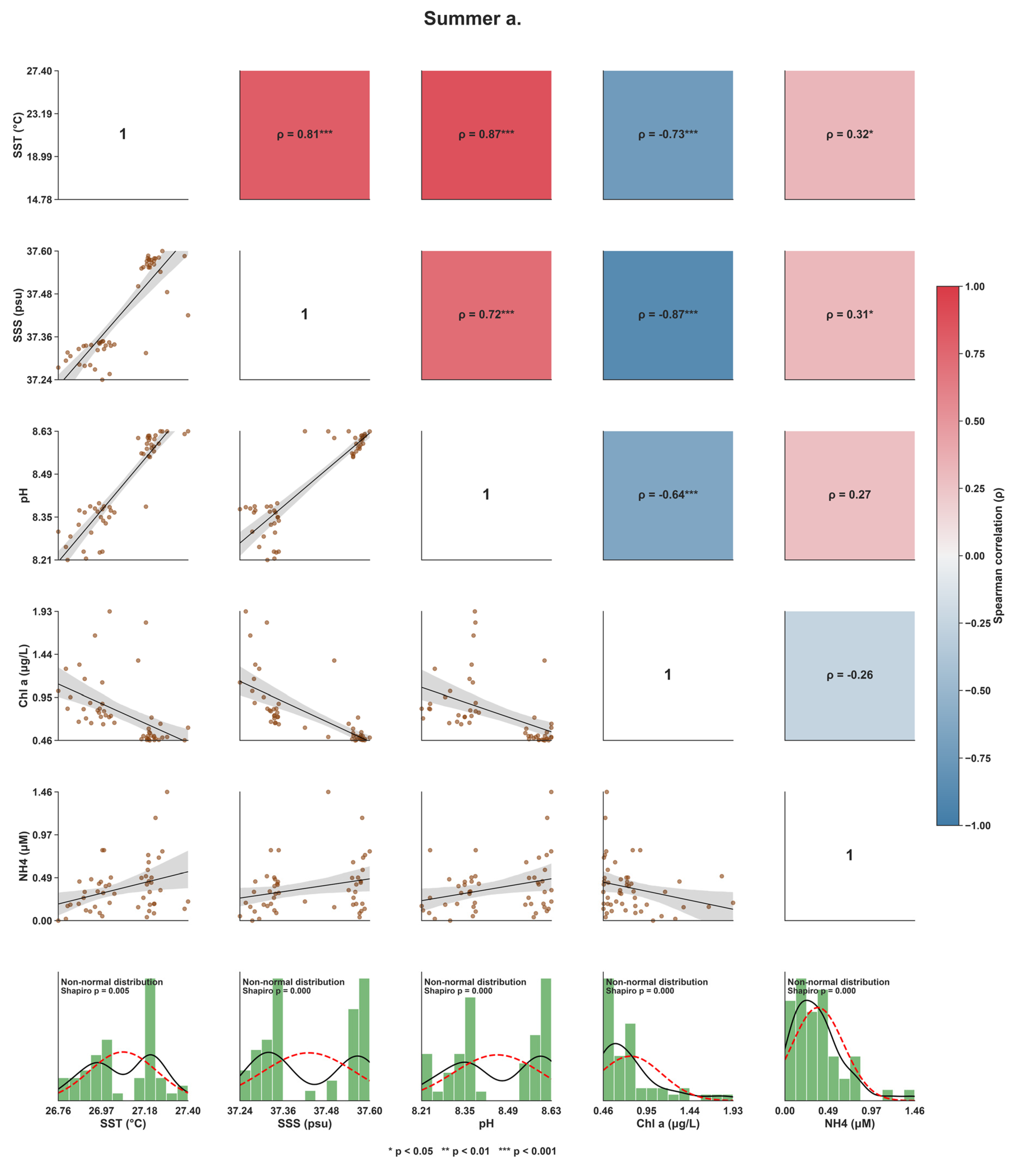
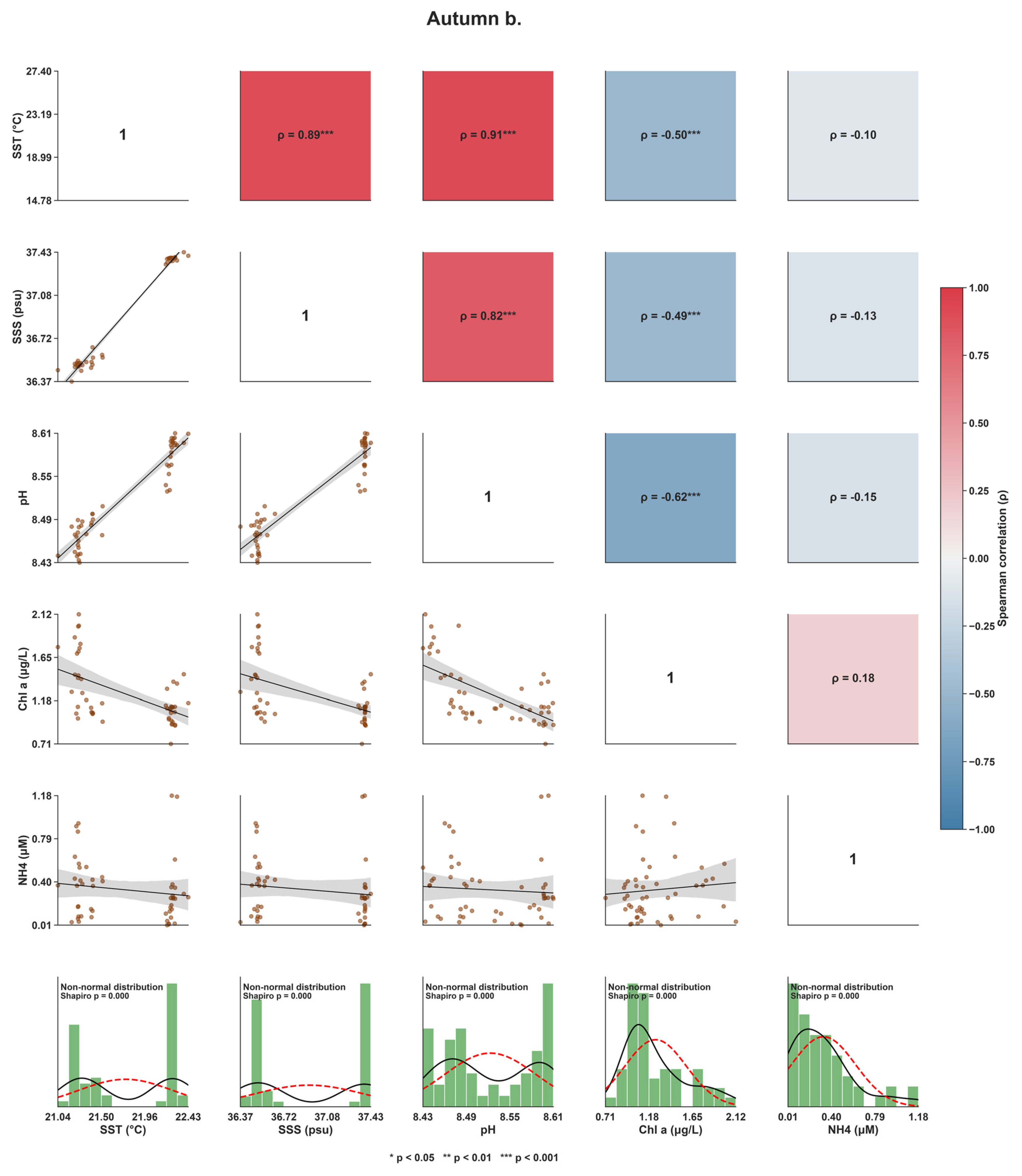
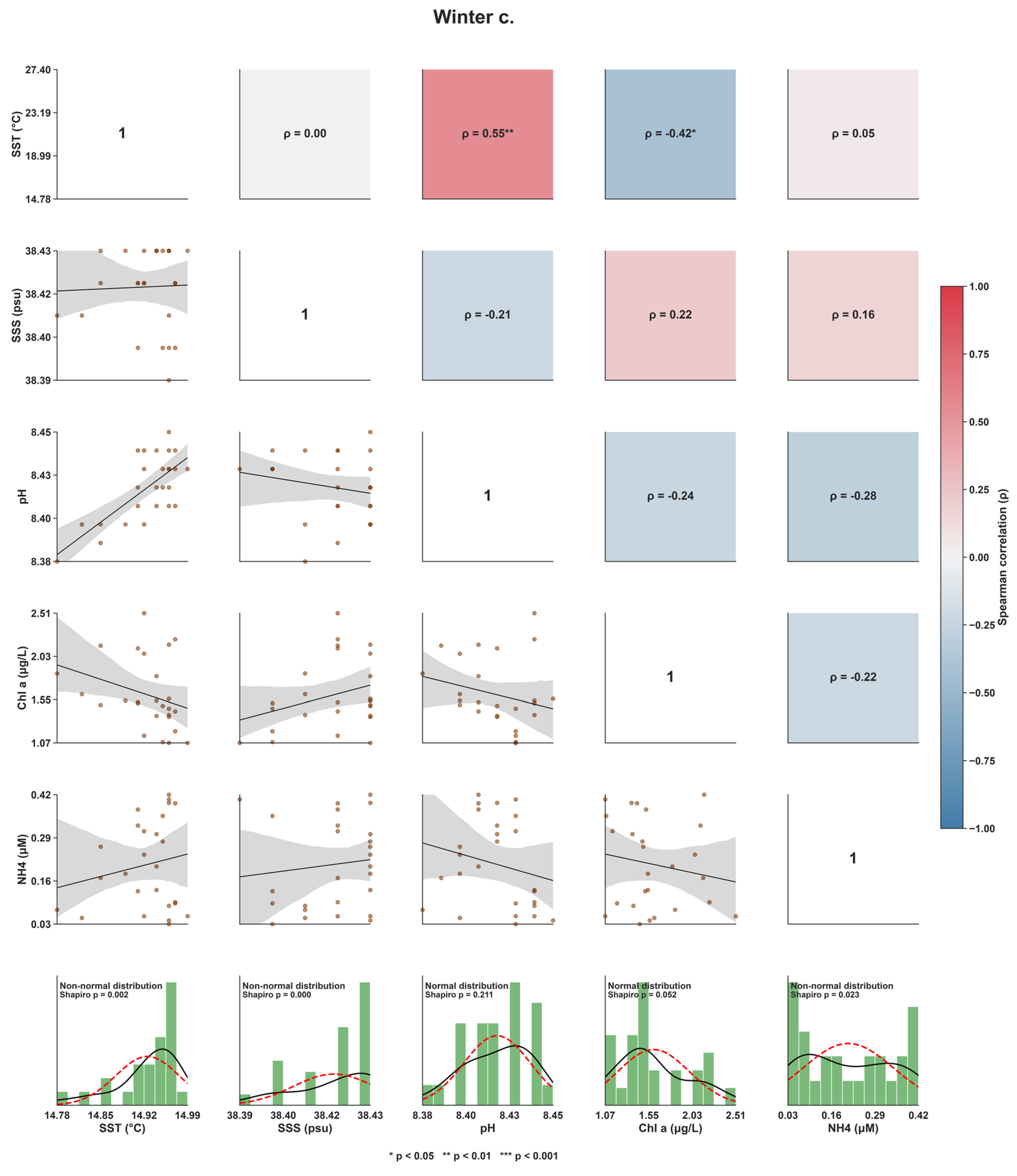
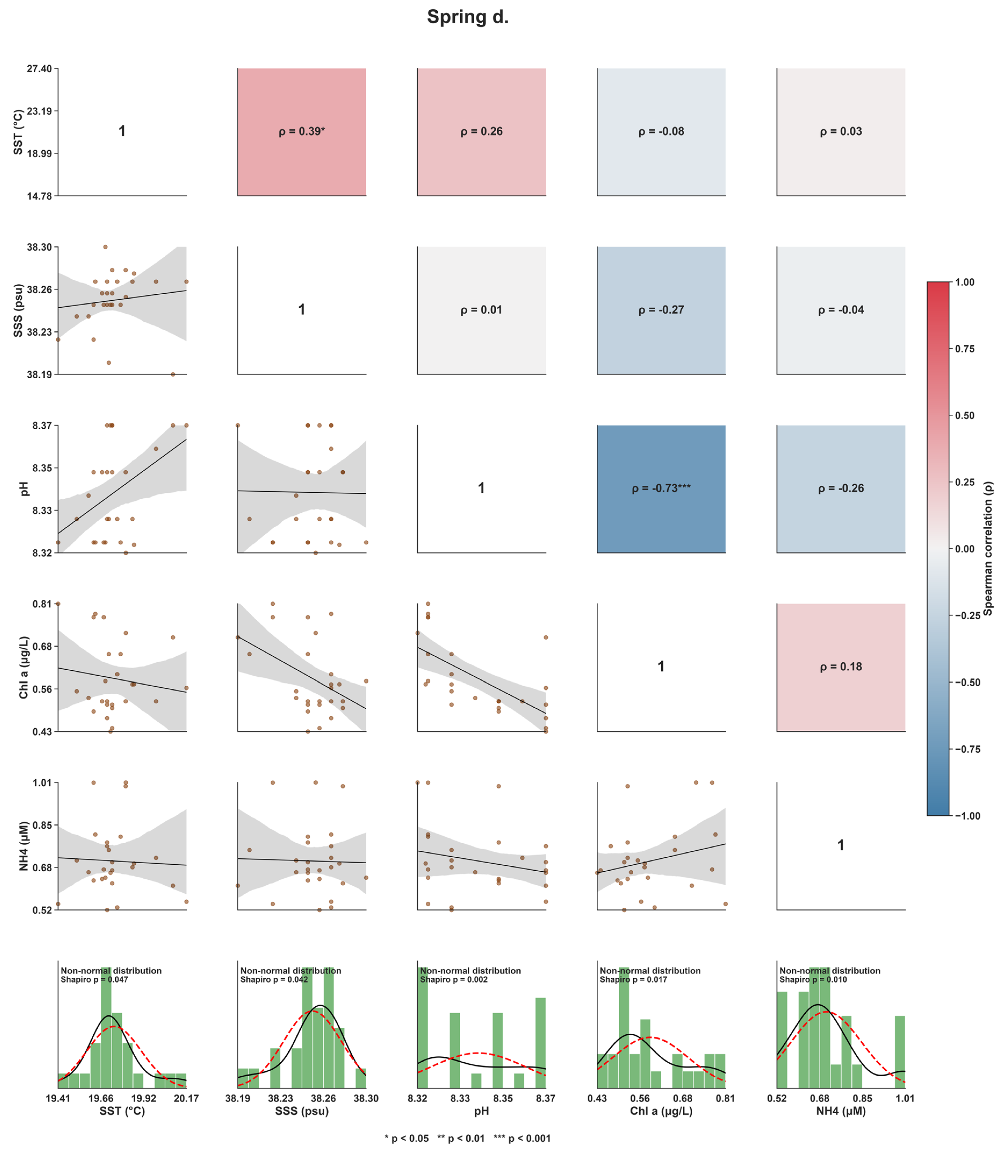
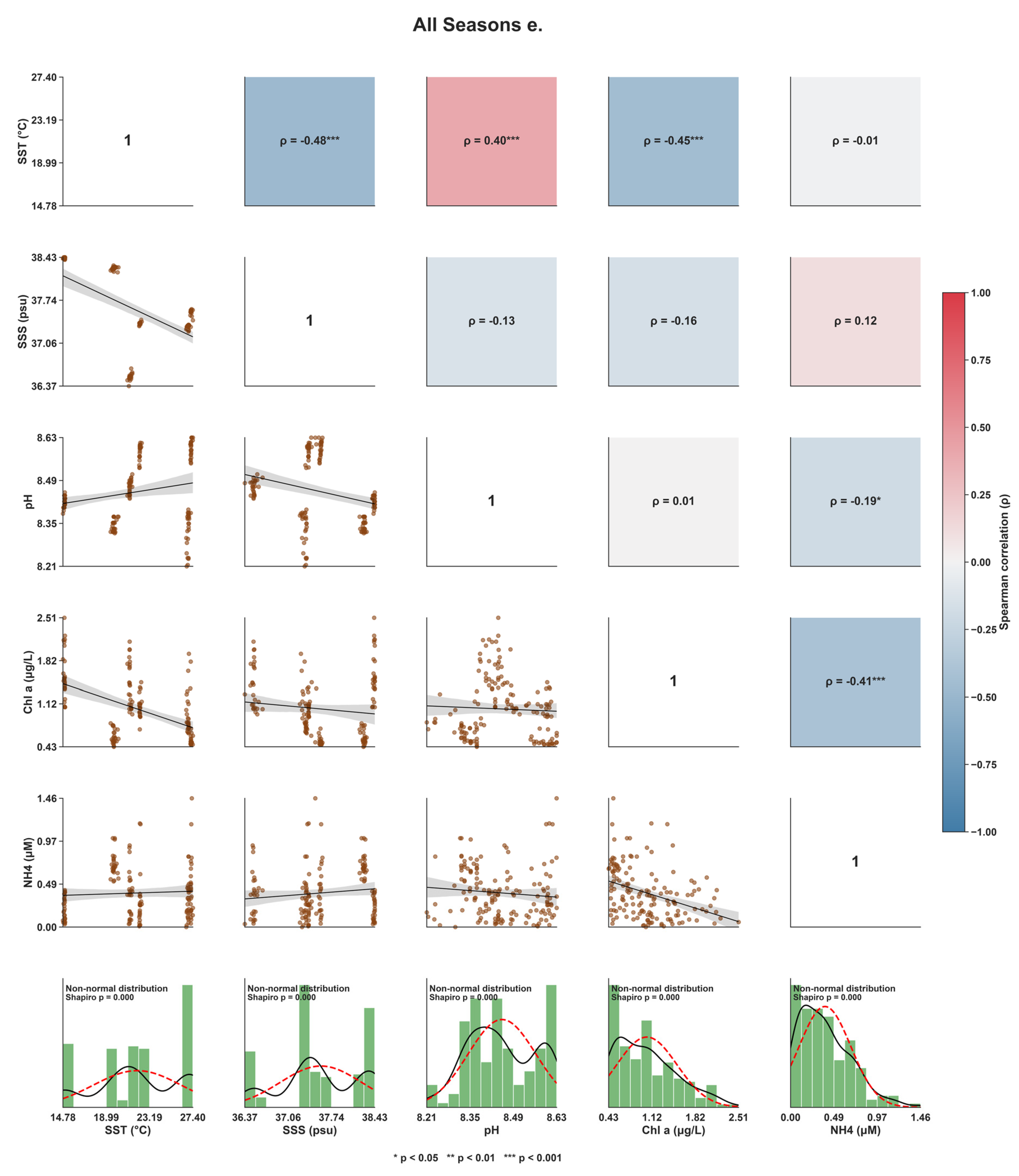
Figure 2.
WQPs distribution across different seasons. The central line inside the box represents the median, while the box contains the middle 50% of the data (interquartile range (IQR), Q1-Q3). The larger the box, the greater the dispersion of the observations. The lower and upper whiskers extend to the smallest and largest values, respectively, within the 1.5×IQR from Q1 to Q3. The points represent the outliers (i.e., extreme values) [23].
Figure 2.
WQPs distribution across different seasons. The central line inside the box represents the median, while the box contains the middle 50% of the data (interquartile range (IQR), Q1-Q3). The larger the box, the greater the dispersion of the observations. The lower and upper whiskers extend to the smallest and largest values, respectively, within the 1.5×IQR from Q1 to Q3. The points represent the outliers (i.e., extreme values) [23].
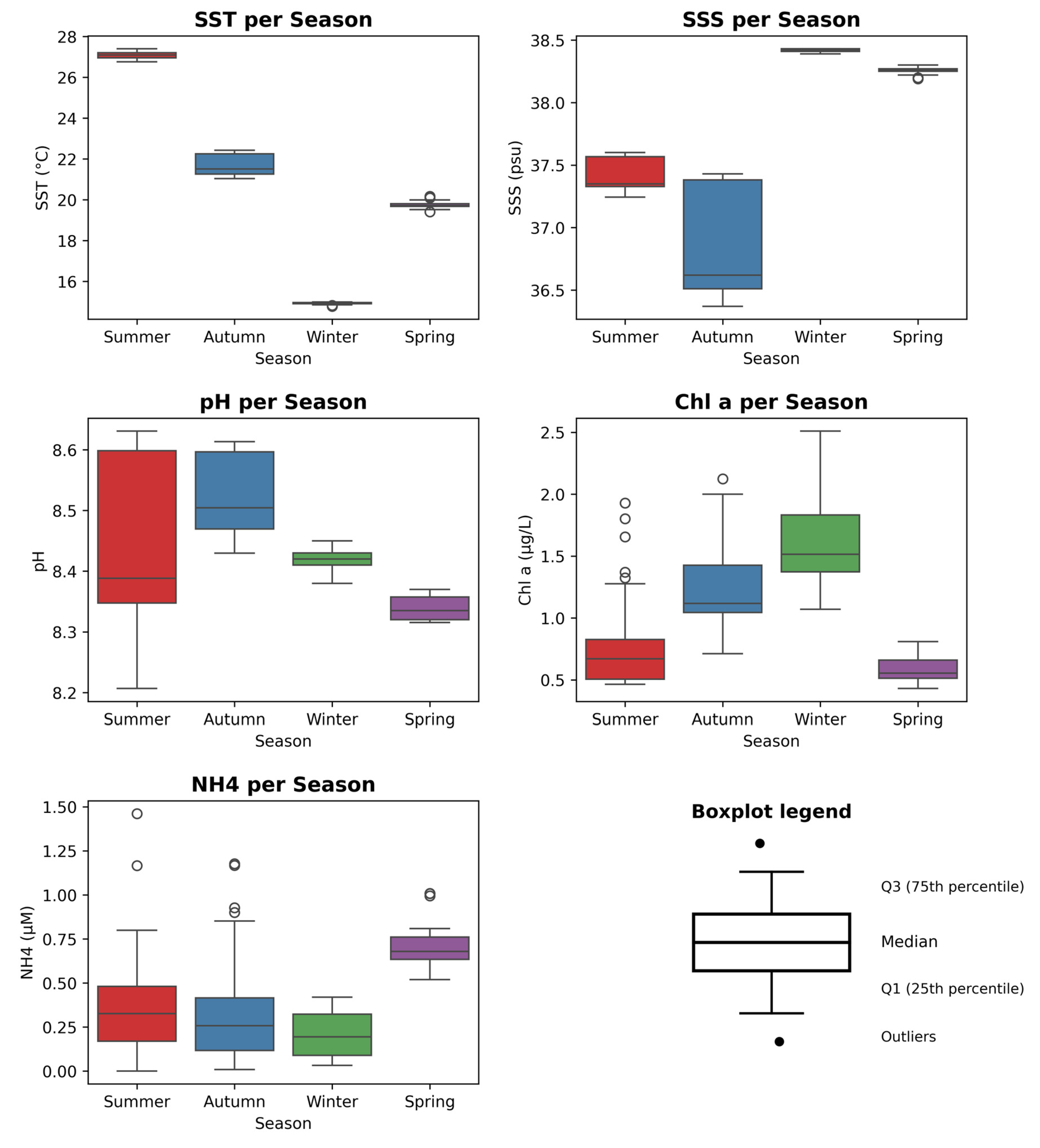
Figure 3.
Multicollinearity assessment of Sentinel-2 MSI spectral bands using Variance Inflation Factor (VIF).
Figure 3.
Multicollinearity assessment of Sentinel-2 MSI spectral bands using Variance Inflation Factor (VIF).
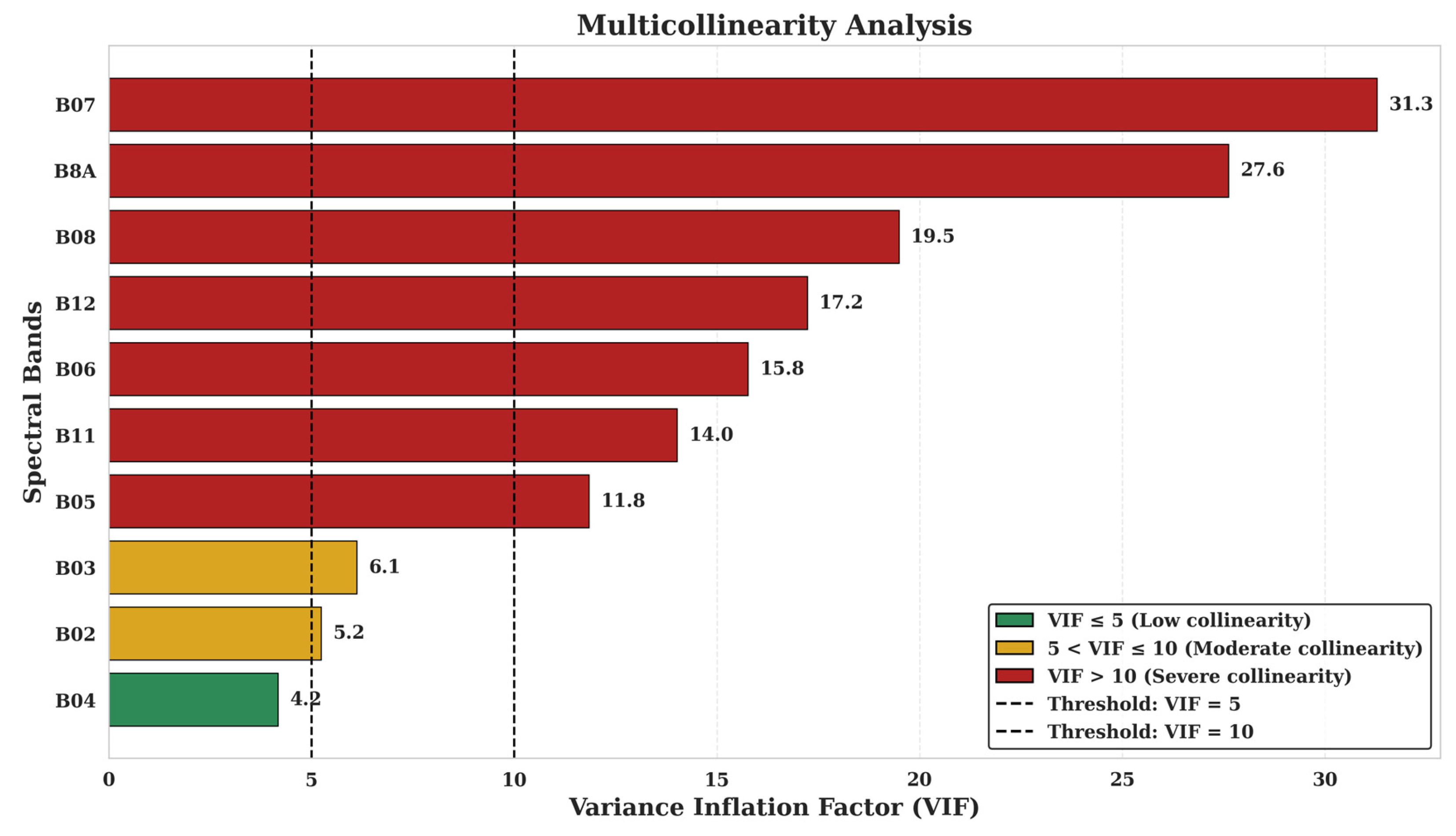
Figure 4.
Spearman’s correlation analysis (ρ) of Sentinel-2 MSI spectral bands and NH4+ concentrations.
Figure 4.
Spearman’s correlation analysis (ρ) of Sentinel-2 MSI spectral bands and NH4+ concentrations.
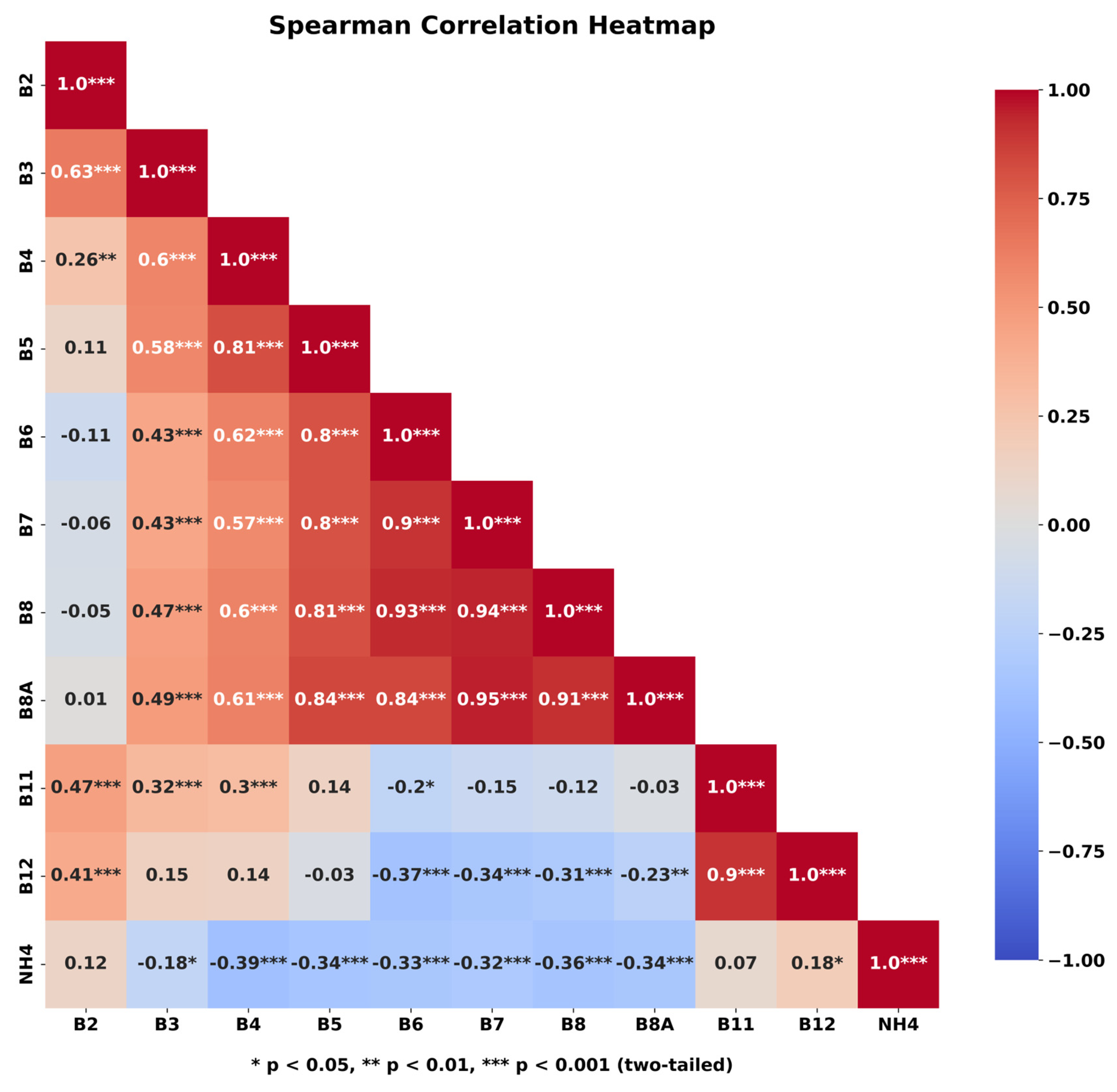
Figure 5.
Spectral bands identified through band-selection procedure and their relative importance in NH4+ estimation.
Figure 5.
Spectral bands identified through band-selection procedure and their relative importance in NH4+ estimation.
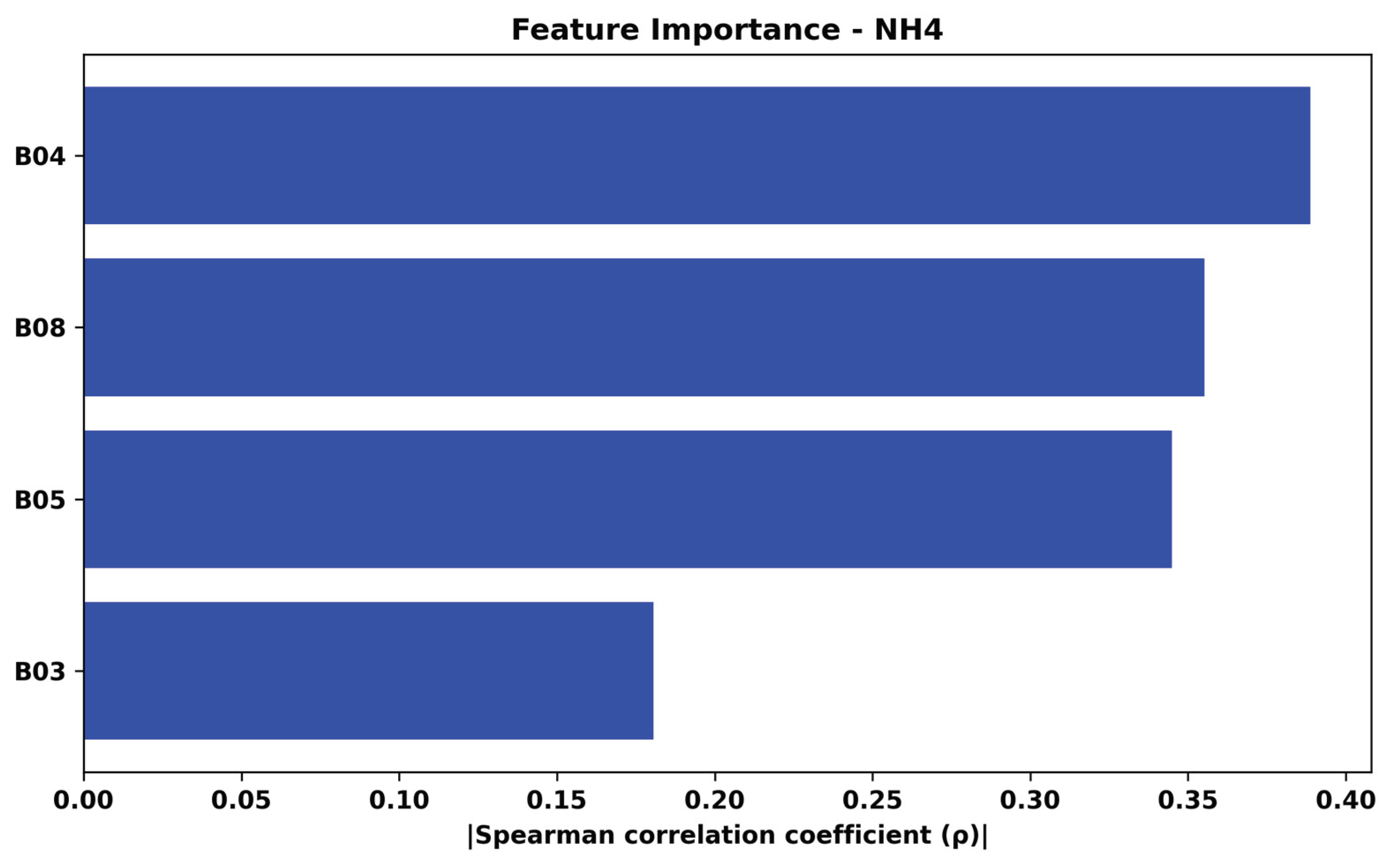

Table 1.
Minimum, maximum and mean ± standard deviation (SD) of in situ SST, SSS, pH, chl a and NH4+ measurements across different seasons.
Table 1.
Minimum, maximum and mean ± standard deviation (SD) of in situ SST, SSS, pH, chl a and NH4+ measurements across different seasons.
| WQP | SUMMER | AUTUMN | WINTER | SPRING |
| SST (oC) | ||||
| Range | 26.76-27.40 | 21.04-22.43 | 14.78-14.99 | 19.41-20.17 |
| Mean ± SD | 27.08 ± 0.17 | 21.76 ± 0.49 | 14.93 ± 0.05 | 19.74 ± 0.16 |
| SSS (psu) | ||||
| Range | 37.24-37.60 | 36.37-37.43 | 38.39-38.43 | 38.19-38.30 |
| Mean ± SD | 37.43 ± 0.13 | 36.93 ± 0.44 | 38.42 ± 0.01 | 38.25 ± 0.02 |
| pH | ||||
| Range | 8.21-8.63 | 8.43-8.61 | 8.38-8.45 | 8.32-8.37 |
| Mean ± SD | 8.45 ± 0.14 | 8.52 ± 0.06 | 8.42 ± 0.02 | 8.34 ± 0.02 |
| Chl a (μg/L) | ||||
| Range | 0.46-1.93 | 0.71-2.12 | 1.07-2.51 | 0.43-0.81 |
| Mean ± SD | 0.77 ± 0.35 | 1.26 ± 0.33 | 1.60 ± 0.39 | 0.59 ± 0.11 |
| NH4+ (μM) | ||||
| Range | 0.00-1.46 | 0.01-1.18 | 0.03-0.42 | 0.52-1.01 |
| Mean ± SD | 0.37 ± 0.29 | 0.33 ± 0.29 | 0.21 ± 0.13 | 0.71-0.13 |
Table 2.
Pairwise seasonal differences in SST, SSS, pH, chl a and NH4+ based on Dunn’s (z) test.
| Season | Summer | Autumn | Winter | Spring | WQP |
| Summer |  |
|
|
SST | |
| Autumn | |
|
|||
| Winter |  |
||||
| Spring | |||||
| Season | Summer | Autumn | Winter | Spring | WQP |
| Summer | |
|
|
SSS | |
| Autumn | |
|
|||
| Winter | |
||||
| Spring | |||||
| Season | Summer | Autumn | Winter | Spring | WQP |
| Summer | |
|
|
pH | |
| Autumn | |
|
|||
| Winter | |
||||
| Spring | |||||
| Season | Summer | Autumn | Winter | Spring | WQP |
| Summer | |
|
|
chl a | |
| Autumn | |
|
|||
| Winter | |
||||
| Spring | |||||
| Season | Summer | Autumn | Winter | Spring | WQP |
| Summer | |
|
|
NH4+ | |
| Autumn | |
|
|||
| Winter | |
||||
| Spring |
Significant differences (p < 0.05), Non-significant differences.
Table 3.
Assessment of ML models’ generalization ability using the difference in the coefficient of determination (ΔR2) and overfitting ratios (ORRMSE and ORMAE).
Table 3.
Assessment of ML models’ generalization ability using the difference in the coefficient of determination (ΔR2) and overfitting ratios (ORRMSE and ORMAE).
| Model | Spectral Bands | ΔR2 | ORRMSE | ORMAE | Overfitting Assessment |
| XGBoost (PSO) | All | 0,53 | 1,80 | 1,77 | High Overfitting |
| B03, B04, B05, B08 | 0,45 | 1,52 | 1,38 | High Overfitting | |
| RF (BO-TPE) | All | 0,29 | 1,30 | 1,29 | High Overfitting |
| B03, B04, B05, B08 | 0,07 | 1,11 | 1,02 | Low Overfitting | |
| SVR (BO-TPE) | All | 0,21 | 1,21 | 1,15 | Moderate Overfitting |
| B03, B04, B05, B08 | 0,07 | 1,10 | 1,01 | Low Overfitting |
Disclaimer/Publisher’s Note: The statements, opinions and data contained in all publications are solely those of the individual author(s) and contributor(s) and not of MDPI and/or the editor(s). MDPI and/or the editor(s) disclaim responsibility for any injury to people or property resulting from any ideas, methods, instructions or products referred to in the content. |
© 2026 by the authors. Licensee MDPI, Basel, Switzerland. This article is an open access article distributed under the terms and conditions of the Creative Commons Attribution (CC BY) license (http://creativecommons.org/licenses/by/4.0/).
Copyright: This open access article is published under a Creative Commons CC BY 4.0 license, which permit the free download, distribution, and reuse, provided that the author and preprint are cited in any reuse.