

Submitted:
14 August 2026
Posted:
14 August 2026
You are already at the latest version
Abstract
The numerical simulation of incompressible viscous flows remains a central pillar of modern computational fluid dynamics (CFD). Over the past decades, a wide spectrum of numerical methodologies has been developed, reflecting fundamentally different mathematical formulations and discretization philosophies. Among these, domain-based approaches—including finite difference (FDM), finite volume (FVM), and finite element (FEM) methods—have emerged as versatile and general-purpose frameworks, while boundary element methods (BEM) provide efficient alternatives for selected classes of problems governed by linear physics, particularly in unbounded domains. Meshfree and particle-based methods constitute an alternative paradigm for problems involving large deformation, moving interfaces, free surfaces, and fragmentation. This review provides a unified comparison of FDM, FVM, FEM, BEM, and meshfree approaches, emphasizing their mathematical foundations, treatment of nonlinear operators, stability, consistency, convergence, computational characteristics, and compatibility with turbulence modeling. Particular attention is given to the interaction between discretization and Reynolds-averaged Navier– Stokes(RANS), large-eddy simulation (LES), direct numerical simulation (DNS), and hybrid RANS–LES methodologies, including detached-eddy simulation (DES), delayed detached-eddy simulation (DDES), improved delayed detached-eddy simulation (IDDES), and stress-blended eddy simulation (SBES). Recent developments in highorder discretization, immersed-boundary and hybrid formulations, meshfree methods, and artificial-intelligence-assisted CFD are also discussed. The review demonstrates that no numerical method is universally optimal; rather, methodological suitability is governed by the interplay among flow physics, Reynolds number, geometry, boundary conditions, and computational requirements.
Keywords:
computational fluid dynamics
; Newtonian fluids
; incompressible viscous flows
; domain discretization methods
; boundary integral methods
; meshless methods
MSC: 76-XX (Fluid mechanics), specifically 76Mxx (Basic methods in fluid mechanics)
1. Introduction
The numerical simulation of incompressible viscous flows of Newtonian fluids governed by the Navier– Stokes equations, is indeed essential to modern computational fluid dynamics (CFD). These aforementioned nonlinear partial differential equations of elliptic type, generally require discrete algebraic frameworks through which the continuous flow variables can be approximated at discrete points in space and time [1,2]. Depending on the mathematical formulation, numerical approaches can be broadly divided into domain-based methods, such as the finite difference method (FDM), finite volume method (FVM), and finite element method (FEM), boundary-based formulations such as the boundary element method (BEM), and meshfree or particle-based approaches [3]. The distinction among these methodologies is not merely related to the geometry of the computational grid. Each method is associated with a particular mathematical representation of the governing equations and consequently with different mechanisms for handling nonlinear operators, boundary conditions, conservation properties, stability, and convergence. FDM approximates differential operators directly, FVM derives discrete equations from integral conservation laws over control volumes, FEM is commonly based on weak or variational formulations, and BEM transforms selected differential equations into boundary integral equations. Meshfree methods, in turn, avoid predefined mesh connectivity and employ scattered nodes, particles, kernels, or moving-least-squares approximations [3]. Recent mathematical developments have also emphasized the relationship between formulation, discretization, and convergence. Gauge formulations and high-order finite-difference approaches, for example, have been investigated for incompressible viscous flows, while stabilized and multiscale finite-element formulations have been developed for convection-dominated problems [4,5,6]. Meshfree and Lagrangian methods offer distinctive advantages for complex interface deformations, fluid–structure interaction (FSI), fragmentation, and violent free surface flows. Recent particle-based developments have extended these capabilities to highly transient incompressible-flow problems [7]. Recent developments in artificial intelligence (AI) and machine learning (ML) have further expanded the CFD landscape. Data-driven turbulence closures, physics-informed machine learning, neural operators, machine-learning-assisted numerical methods, and accelerated CFD algorithms are increasingly being investigated [8,9,10,11,12,13,14]. These developments introduce new possibilities for turbulence modeling, reduced order representations, adaptive discretization, and solver acceleration. Nevertheless, physical consistency, numerical stability, conservation, and generalization remain essential requirements when data-driven models are coupled with conventional CFD algorithms. Beyond the classical formulation, mathematical modifications concerning the structural form of the governing equations and the precise physical conditions under which their transport terms are evaluated have also been the subject of continued investigation. In particular, in Ref. [15] a modified form of the Navier– Stokes equations for three-dimensional flows and examined the associated mathematical framework under specified spatial parameters was presented. This work provides an example of how modifications to the mathematical structure of the governing equations may affect the formulation of incompressible-flow problems. Moreover, in Ref. [16] a computational study was performed to examine the three-dimensional turbulent wind flow around two square buildings featuring pyramid roofs. The simulation addressed the fundamental aerodynamic problem of an external turbulent flow field past successive obstacles, one behind the other, with strict geometric placement and predefined shape. The core novelty of this research is the rigorous theoretical demonstration of grid independence. This mathematical proof eliminates the standard requirement for physical grid refinement and consecutive, repetitive computational runs.
Further, a fundamental physical distinction in incompressible fluid mechanics is that between external and internal flows. External flows occur around bodies in effectively unbounded domains, whereas internal flows occur within confined geometries such as pipes, channels, cavities, and industrial process equipment [17,18]. The appropriate numerical method depends strongly on this distinction, but also on Reynolds number, geometry, linearity, boundary conditions, and the physical scales that must be resolved. The increasing importance of high-Reynolds-number and multiphysics simulations has favored domain-based formulations because nonlinear transport and turbulence are fundamentally volumetric phenomena. High-order FVM and stabilized or variational multiscale FEM formulations provide substantial flexibility in such applications, whereas classical BEM becomes less attractive when nonlinear volume terms must be evaluated explicitly. Conversely, BEM retains important advantages for selected classes of linear problems, particularly low-Reynolds-number hydrodynamics and exterior problems. Meshfree approaches offer complementary advantages in problems involving moving boundaries, free surfaces, and large deformation. The objective of the present review is therefore to provide a rigorous and unified comparison of FDM, FVM, FEM, BEM, and meshfree approaches for incompressible viscous flows of Newtonian fluids, with particular emphasis on their mathematical foundations, nonlinear operators, stability, convergence, turbulence compatibility, and computational characteristics.
2. Governing Equations and Mathematical Foundations
2.1. Governing Equations
The mathematical baseline of the present comparative study is the three-dimensional, unsteady, incompressible Navier–Stokes system for a Newtonian fluid. In vector notation, the continuity equation is
while the momentum equation is
where u is the velocity vector, ρ is the constant density, (p) is pressure, μ is the dynamic viscosity, and f represents body forces.
∇ · u = 0
ρ(∂u/∂t + (u · ∇)u) = -∇p + μ∇²u + f
The nonlinear convective acceleration term (u · ∇)u) which actually is a pseudovector operator is particularly important in the comparison of numerical methods because it is a volumetric nonlinear operator. Its numerical treatment becomes increasingly demanding with increasing Reynolds number.
2.2. Strong and Weak Formulations
A fundamental distinction exists between strong and weak formulations. In the strong formulation, the governing differential equations are required to hold pointwise throughout the computational domain, subject to the prescribed boundary and initial conditions. Classical finite-difference schemes are closely associated with this formulation. In a weak formulation, the governing equations are multiplied by suitable test functions and integrated over the computational domain. Integration by parts may then transfer derivatives from the unknown field to the test functions.
This reduces the differentiability requirements and forms the mathematical basis of many finite element and meshfree formulations.
Schematically, one may write out
where
Ω: The integration domain or space.
v, f: Functions or variables defined on the domain.
dΩ: The differential volume, area, or measure element.
Here one may emphasize that the distinction between strong and weak formulations affects boundary-condition treatment, regularity requirements, stabilization, and the structure of the resulting algebraic system.
2.3. Consistency, Stability, and Convergence
Numerical methods must satisfy appropriate consistency, stability, and convergence requirements. A discretization is consistent when its truncation error tends toward zero as the characteristic discretization length tends toward zero. Stability requires that numerical perturbations and discretization errors remain appropriately bounded. For linear well-posed problems, the Lax equivalence principle establishes the central relationship between consistency, stability, and convergence. Gauge formulations and high-order incompressible-flow discretizations provide additional examples of the development of numerical techniques designed to improve these properties [4,5]. For nonlinear Navier–Stokes simulations, however, stability must be considered at the level of the complete numerical algorithm. Pressure–velocity coupling, nonlinear convection, boundary conditions, temporal discretization, turbulence closure, and stabilization can all influence the behavior of the discrete system.
3. Historical Development of Numerical CFD Methods
The development of numerical methods for incompressible viscous flows has progressed in parallel with advances in applied mathematics, numerical analysis, and computer technology. During the 1950s and 1960s, early computational approaches relied heavily on finitedifference approximations of the Navier–Stokes equations. A major milestone was the Marker-and-Cell (MAC) method of Harlow and Welch [19], which provided an important framework for time-dependent incompressible flow and free-surface problems. Projection and fractional-step methods subsequently addressed pressure–velocity coupling. Chorin introduced a projection method for the incompressible Navier– Stokes equations [20], while Kim and Moin developed a fractional-step formulation that remains influential in modern incompressible solvers [21]. The mathematical analysis of difference methods developed in parallel. Classical numerical-analysis treatments established the foundations for consistency, stability, and convergence [22,23]. During the 1970s and 1980s, finite-element and finite-volume approaches expanded CFD capabilities. FEM provided substantial geometric flexibility through variational formulations [24,25], while FVM emphasized direct enforcement of conservation laws through integral balance equations [26]. Boundary-integral methods developed in parallel. By exploiting fundamental solutions, BEM transforms selected differential equations into equations defined on the boundary [27,28,29]. This feature proved particularly advantageous for Stokes flow and exterior problems. During the 1990s and 2000s, unstructured meshes, high-performance computing, adaptive methods, and large-scale simulations became increasingly important. At the same time, meshfree and particle-based methods emerged in response to difficulties associated with conventional mesh generation and moving interfaces [30,31,32]. More recently, high-order methods, immersed-boundary formulations, hybrid Eulerian–Lagrangian approaches, advanced turbulence modeling, and data-driven CFD have become major research directions [33,34,35,36,37,38,39,40]. The historical evolution of CFD thus reflects a continuous interplay between mathematical formulation, computational capability, and the physical complexity of fluid flows. In Table 1 a brief timeline regarding the key developments in CFD methods in the period 1950–2020 is presented
From a historical standpoint, the current predominance of domain discretization methods in CFD should therefore be understood not as a rejection of boundary-based techniques, but as the outcome of a natural co-evolution between physical modeling requirements and computational capability. Boundary element methods remain valuable within their domain of applicability; however, the expansion of CFD into turbulence-dominated and industrially relevant regimes has firmly established domain discretization methods as the principal computational paradigm.
Overall, the historical progression of CFD methodologies reflects a continuous effort to balance mathematical rigor, computational efficiency, and physical realism.
4. Domain Discretization Methods
In general, one may elucidate that all governing conservation equations of transport phenomena are able to be represented in the following comprehensive form:
or equivalently
where ρ is the density of air or mixture (if chemical species are present), t is the time, u is the velocity vector, Γφ is the diffusion coefficient of the transported quantity, Sφ is the source or sink term and φ is the general transported quantity.
4.1. Finite Difference Method
The finite difference method approximates differential operators using algebraic combinations of neighboring nodal values. Taylor-series expansions provide the classical basis for deriving such approximations.
For example,
This equation defines the second-order central finite difference approximation for a second-order partial derivative. It is a fundamental numerical method used to discretize differential equations on a spatial grid, commonly implemented in computer simulations for physics and engineering applications
FDM is conceptually simple and computationally efficient, particularly on structured grids. Its regular matrix structure can be exploited efficiently using modern sparse solvers and parallel architectures. High-order finite-difference methods are particularly attractive for DNS and LES because they can provide low numerical dissipation and favorable dispersion characteristics. Fourth-order formulations have been investigated for unsteady incompressible viscous problems [5]. The principal limitation of FDM is geometric flexibility. Complex curved boundaries and irregular domains generally require coordinate transformations, immersed boundary techniques, or specialized boundary treatments. Consequently, FDM remains highly competitive for canonical configurations such as channels, pipes, cavities, and homogeneous turbulence, while FVM and FEM generally provide greater flexibility for complex industrial geometries
4.2. Finite Volume Method
The finite volume method (FVM) is based directly on the integral form of conservation laws. The two primary governing equations are the continuity equation (conservation of mass) and the momentum equation (conservation of momentum). The computational domain is divided into control volumes and the governing transport equations are integrated over each volume. The mass and momentum conservation equations for an incompressible flow are represented in integral form over a discrete control volume V bounded by a surface S
where
is the total volume of cell
is the velocity vector evaluated at the cell center.
is the mass flow rate passing through cell face subscript denotes values interpolated or reconstructed at the cell face centers from adjacent cell centers
In this context, in order to implement FVM to incompressible flows of Newtonian fluids, one should primarily focus on how the continuous surface integrals are converted into linear algebraic equations and how the pressure-velocity coupling is handled. The divergence theorem converts volume derivatives into surface fluxes. The direct connection between the numerical equations and the conservation laws is a principal strength of FVM [26]. Modern formulations can employ structured, unstructured, hybrid, and polyhedral meshes. The principal challenge is to obtain high-order accuracy while maintaining conservation, boundedness, and robustness on irregular meshes. Moreover, one may observe that in incompressible flows, density is constant. Actually, there is no explicit transport equation for pressure, nor does pressure appear in the continuity equation. Instead, pressure acts as a mathematical constraint to ensure the velocity field remains divergence-free.
In addition, one may elucidate that since pressure does not explicitly appear in the mass conservation constraint for incompressible flows, numerical schemes like SIMPLE, PISO, or PIMPLE are utilized to couple the velocity fields and pressure forces safely without causing odd-even grid decoupling.
4.3. Finite Element Method
The finite element method is based on variational or weighted-residual formulations. The numerical solution may be represented as
where (Ni) are basis functions. The weak formulation provides substantial flexibility for complex geometries and multiphysics problems [24,25].
u(x) ≈ ∑i{i=1}^{N} Ni(x) ui
The above expression represents a linear combination of spatial basis functions (or shape functions) and discrete nodal coefficients. Unstructured meshes can represent complex domains efficiently. For incompressible flow, pressure–velocity coupling introduces an important mathematical constraint. Appropriate velocity and pressure spaces must satisfy relevant stability conditions, while stabilized formulations and variational multiscale approaches improve the treatment of convection-dominated and turbulent flows [6]. FEM is therefore particularly attractive for complex geometries, fluid–structure interaction, multiphysics, and high-order formulations. Nonetheless, in order for the application of this method to unbounded domains, the contrivance of artificial boundaries is generally demanded. Here, one has to assume beforehand that either the shape of the real boundary or the rates of a field quantity along the artificial boundary are considered as known beforehand. Yet, the creation of a finite element grid constitutes a difficult geometrical problem, perhaps more difficult as it was proved than the circumstantial physical problem that a CFD method is called to solve.
5. Boundary Element Method
The boundary element method represents a fundamentally different numerical philosophy. Rather than discretizing the complete computational domain, selected governing equations are transformed into boundary integral equations using Green's functions or fundamental solutions [27,28,29].
In fluid dynamics and continuum mechanics, the Boundary Element Method (BEM) handles mass and momentum conservation by transforming the governing partial differential equations (PDEs) into boundary integral equations.
Since BEM relies on analytical "fundamental solutions" (Green's functions), it is most powerful for linear, steady-state, or incompressible flows, such as Stokes flow (creeping flow) or Potential flow.
In BEM, the governing partial differential equations are transformed into boundary integral equations using a known linear fundamental solution—in this case, the steady-state Stokeslet tensors. The unsteady and non-linear convective terms are treated as pseudo-body forces on the right-hand side and converted to the boundary via radial basis functions. Given a source point named and a moving field point named , the localized mass and momentum conservation balances can be represented by means of the following fundamental boundary integral equation
where
denotes velocity vector component
the boundary transition vector component
he boundary geometric tensor
; velocity and traction tensors respectively
The principal computational advantage is dimensional reduction. A three-dimensional problem may be represented through a two-dimensional boundary discretization. BEM is therefore particularly attractive for potential flow, linear elasticity, Stokes flow, low-Reynolds-number hydrodynamics, and selected multiphysics problems. Its main limitation arises from nonlinear volumetric terms. Moreover one may pinpoint that the Navier–Stokes convective operator is intrinsically volumetric. Consequently, exact reduction of a general nonlinear Navier–Stokes problem to a purely boundary representation is not generally possible. Boundary–domain formulations can be used, but these require additional volume treatment. This limitation becomes even more important for turbulence because Reynolds stresses and subgrid-scale stresses represent volumetric transport phenomena. Thus, BEM should not be viewed as a general-purpose replacement for FVM or FEM in high-Reynolds-number turbulent CFD. Its strongest role remains in specialized regimes characterized by linearity, low Reynolds number, or unbounded domains. Next, Table 2 illustrates a rough comparison between BEM and FEM
6. Meshfree and Particle-Based Methods
Meshfree methods avoid predefined mesh connectivity and approximate the solution using scattered nodes, particles, kernels, or moving-least-squares procedures [3,30,31,32]. Smoothed particle hydrodynamics (SPH) is one of the best-established particle methods.
A generic field approximation can be expressed as
where W is a smoothing kernel,
f(x) ≈ ∑j fj W(x - xj, h) Vj
h is the characteristic smoothing length,
Vj is the particle volume.
The principal advantage of meshfree methods is their geometric flexibility. Particles can naturally follow interfaces, free surfaces, and strongly deforming material regions without requiring conventional remeshing. Applications include free-surface flows, multiphase flows, violent wave impact, fragmentation, moving boundaries, and fluid–structure interaction. Incompressible SPH formulations have been developed specifically to improve pressure stability and free-surface accuracy [43]. Generalized wall boundary conditions have also been proposed [44]. Recent meshless formulations have further addressed highly transient green-water and free-surface events through volume-conservative Lagrangian formulations and weighted-least-squares spatial operators [45]. Other formulations have investigated generalized meshless approaches to incompressible Navier–Stokes equations [46]. Despite these advances, meshfree methods remain challenged by particle disorder, consistency, boundary treatment, pressure stabilization, and computational cost.
7. Turbulence Modeling and Its Interaction with Discretization
Turbulence modeling is intrinsically linked to numerical discretization. RANS, LES, and DNS introduce fundamentally different requirements for spatial resolution, temporal accuracy, and physical modeling [33,34,35]. RANS approaches model the statistical effect of turbulence and require closure relations for Reynolds stresses. LES resolves large turbulent structures and models the effect of unresolved scales, whereas DNS attempts to resolve all dynamically relevant scales [33,34,35]. Domain discretization methods provide a natural framework for these approaches because turbulent transport is volumetric and nonlinear. FVM and FEM are widely used in RANS and LES because of their conservation properties, geometric flexibility, and compatibility with turbulence models. FDM has played a particularly important role in DNS of canonical flows because structured grids and high-order operators can provide excellent computational efficiency. The integration of turbulence modeling into classical BEM is more limited. Turbulent stresses and nonlinear convection are volumetric and therefore cannot generally be represented solely through classical boundary integrals. Hybrid boundary–domain formulations are possible, but their volume treatment reduces the dimensional reduction advantage of BEM. Meshfree methods have also been extended to turbulent flows, including SPH-based LES approaches. Their Lagrangian character is attractive for free-surface and strongly transient flows, but accurate treatment of incompressibility and wall-bounded turbulence remains challenging. The central conclusion is therefore that turbulence modeling and discretization should not be treated as independent choices.
8. External and Internal Incompressible Flows
External flows involve fluid motion around bodies in effectively unbounded domains. At low Reynolds numbers, such flows may approach Stokes regimes, for which boundary-integral formulations are particularly natural and efficient [29]. In creeping external flows, BEM can calculate hydrodynamic forces and stresses without explicitly discretizing the field. This is a major advantage over conventional domain-based methods. As Reynolds number increases, boundary layers, separation, wakes, and turbulence develop. The importance of nonlinear volumetric transport consequently increases, and domain-based methods become increasingly advantageous. Internal flows occur within confined geometries such as pipes, channels, cavities, and process equipment [17,18]. Even in laminar conditions, pressure gradients and viscous transport involve the complete domain. At high Reynolds numbers, wallbounded turbulence and secondary flows further reinforce the need for volumetric resolution. FDM remains highly efficient for canonical internal-flow configurations. FEM offers substantial flexibility for complex internal geometries, while FVM is particularly attractive for industrial applications because of its conservation properties. Meshfree approaches become especially interesting when internal boundaries deform or move. Thus, method selection should not be based exclusively on the classification as internal or external flow. Reynolds number, linearity, geometry, boundary conditions, and the nature of the transport processes must be considered simultaneously.
9. Advanced Hybrid RANS–LES Frameworks
9.1. Detached Eddy Simulation
Detached Eddy Simulation (DES) was introduced through a modification of the length scale in the Spalart–Allmaras turbulence model [37].
A schematic hybrid length scale can be written as
where (d) is the distance to the nearest wall, CDES is a model constant, and Δ is a characteristic grid length.
min(d, CDES Δ)
The formulation introduces a direct interaction between the turbulence model and the computational grid. If the grid becomes excessively fine within an attached boundary layer, the formulation may transition prematurely toward LES behavior without providing the resolution necessary to resolve the relevant turbulent structures. This may lead to model-stress depletion and grid-induced separation.
9.2. Delayed Detached Eddy Simulation
Delayed Detached Eddy Simulation (DDES) introduced shielding mechanisms designed to reduce the sensitivity of the RANS-to-LES transition to local grid refinement [38]. A generalized hybrid length scale can be written as
where (fd) is a shielding function.
d - f_d max(0, d - CDES Δ)
The objective is to maintain RANS behavior within attached boundary layers while permitting LES behavior in separated regions. The DDES development therefore provides a particularly clear example of the dependence of turbulence modeling on discretization.
9.3. Improved Delayed Detached Eddy Simulation
Improved Delayed Detached Eddy Simulation (IDDES) extends DDES through additional wall-modeling and blending concepts [39]. The objective is to provide a more seamless transition between modeled and resolved turbulent scales while reducing sensitivity to the computational grid and wall treatment. IDDES is particularly relevant to complex industrial flows in which wall-resolved LES would be computationally prohibitive.
Nevertheless, its accuracy remains dependent on appropriate resolution of separated shear layers, wall treatment, and compatibility between numerical dissipation and turbulence modeling.
9.4. Stress-Blended Eddy Simulation
Stress-Blended Eddy Simulation (SBES) represents a further development of hybrid RANS–LES methodology [40].
The schematic stress-blending relation for the Stress-Blended Eddy Simulation (SBES) formulation is expressed as:
where the above terms listed in the order in which they appear in the last equation describe the following:
- The final modeled turbulent stress tensor used in the momentum equations.
- The turbulent stress tensor computed by the underlying RANS model.
- The subgrid-scale (SGS) stress tensor computed by the LES model.
- The core blending function, which varies strictly between 0 and 1.
Here one may pinpoint that:
- =1 The formulation switches completely to RANS mode, typically inside attached boundary layers.
- = 0 The formulation switches completely to LES mode, typically in separated flow regions.
Unlike classic Detached Eddy Simulation (DES) which blends RANS and LES length scales inside the eddy viscosity formulation, SBES blends the stress tensors directly. This prevents intermediate, unphysical eddy viscosities and allows for a much faster, sharper transition from RANS to LES.
Recent work has emphasized the physical consistency of modern hybrid RANS–LES formulations in complex internal separating flows [41], while industrial aerodynamic applications demonstrate the importance of the coupling between turbulence model, grid, and numerical discretization [42].
The development of DES, DDES, IDDES, and SBES therefore illustrates a central point of this review: the numerical discretization is part of the effective turbulence simulation system.
10. Classification of Numerical Methods
Numerical methods for incompressible flows can be classified into three broad categories: 1. Domain discretization methods: FDM, FVM, FEM;
2. Boundary discretization methods: BEM;
3. Meshfree methods: particle- and node-based approaches. Domain-based methods discretize the complete computational field. Boundary methods reduce the dimensionality of selected problems by transferring the governing equations to the boundary. Meshfree methods retain a volumetric representation but eliminate predefined mesh connectivity. Methods can additionally be classified according to: laminar versus turbulent flow; internal versus external flow; steady versus unsteady flow; low versus high Reynolds number; single-phase versus multiphase flow; fixed versus moving geometry. These classifications are complementary rather than mutually exclusive.
11. Comparative Assessment of Numerical Methods
A thorough description of comparative characteristics of the previously mentioned principal numerical methods is performed in Table 3
Actually, it can be said the above comparison demonstrates that no numerical method is universally optimal. FDM provides high efficiency on structured grids. FVM offers a strong combination of conservation and geometric flexibility. FEM provides a rigorous variational framework for complex geometries and multiphysics. BEM offers dimensional reduction and natural treatment of unbounded domains. Meshfree methods provide exceptional flexibility for large deformation and evolving interfaces.
12. Mathematical and Computational Constraints
A detailed description of stability, discretization, and geometric characteristics of the previously mentioned principal numerical methods is illustrated in Table 3

Table 4.
Stability, discretization, and geometric characteristics.
| Framework | Principal stability considerations | Discretization characteristics | Geometric restrictions | Major advantage |
|---|---|---|---|---|
| BEM | Integral formulation and singular-kernel treatment | Boundary approximation | Boundary mesh | Dimensional reduction |
| FDM | CFL and diffusion restrictions | Low- to high-order finite differences | Structured grids advantageous | Computational efficiency |
| FEM | Pressure–velocity compatibility and stabilization | h- and p-refinement | Highly flexible | Complex geometry and multiphysics |
| FVM | Flux boundedness and stability | Conservative control volumes | Highly flexible | Conservation |
| Meshfree | Particle distribution and kernel stability | Kernel/MLS approximation | No predefined mesh | Large deformation |
These properties should be interpreted as methodological tendencies rather than universal mathematical statements. Actual stability depends on the complete spatial discretization, temporal scheme, boundary treatment, solver, and physical model.
13. Recent Advances in CFD Numerical Methods
Recent CFD research has been characterized by substantial progress in high-order discretization, adaptive methods, meshfree techniques, immersed-boundary formulations, hybrid methodologies, and data-driven approaches. High-fidelity simulations based on FVM and FEM remain major tools for turbulent flow prediction, particularly in LES and DNS, where scalability and accurate spatial resolution are critical. High-order CFD methods have developed significantly, providing improved accuracy while seeking to control computational cost [51]. Immersed-boundary methods provide an important strategy for treating complex moving geometries while retaining Eulerian computational frameworks [36].
Meshfree methods have also progressed substantially. Incompressible SPH formulations, improved wall conditions, and generalized particle methods have expanded their applicability to free-surface and multiphase flows [43,44]. Recent work on green-water loading has demonstrated the potential of meshless, Lagrangian, volume-conservative formulations using weighted-least-squares spatial operators for highly transient free-surface events [45]. Further meshless formulations have explored generalized Riemann-solver-based approaches for CFD [46]. Fully meshless formulations have also been investigated for heat-conduction problems on arbitrary three-dimensional geometries [47], while generalized multiscale finite-element methods combined with balanced truncation have been developed for parameter-dependent parabolic problems [48].
These developments, although not all directly concerned with incompressible CFD, illustrate the broader trend toward mesh-independent and reduced-order computational frameworks. Additional developments include meshfree generalized multiscale finite-element approaches [49] and quasi-meshfree formulations for nonlinear solid mechanics [50]. Such developments demonstrate the broader methodological convergence between mesh-based and mesh-independent numerical representations. Overall, recent advances highlight a clear shift toward high-order accuracy, hybridization, adaptivity, and improved turbulence–discretization coupling.
14. Artificial Intelligence and Machine Learning in CFD
Artificial intelligence is increasingly being integrated into CFD at multiple levels. Machine-learning methods have been applied to turbulence modeling, reduced order modeling, numerical acceleration, and data-driven representations of fluid operators [8,9,10,11,12,13,14]. One important application is data-driven turbulence closure. Neural networks can be trained using high-fidelity DNS data to approximate unresolved turbulent stresses. Deep-learning approaches have demonstrated potential for representing complex subgrid-scale behavior [8]. Machine learning has also been used to accelerate CFD computations.
Kochkov et al. demonstrated the potential of machine-learning-assisted computational fluid dynamics [10], while broader studies have reviewed the integration of machine learning into fluid mechanics and CFD [9,12]. Physics-informed machine learning incorporates governing physical equations into the learning process [11]. Neural operators extend the concept by learning mappings between function spaces rather than individual discrete solution vectors [13]. AI can therefore potentially be incorporated into: adaptive mesh refinement; learned error indicators; particle redistribution; kernel optimization; iterative solver acceleration; reduced-order modeling; turbulence closure; surrogate representations of computational operators. However, the incorporation of AI into CFD raises fundamental mathematical issues. A data-driven model may modify the effective numerical operator and consequently influence stability, conservation, consistency, and convergence. AI should therefore be regarded as an augmentation of CFD rather than a replacement for mathematical and numerical analysis.
15. Future Perspectives: Motivations, Prospects, and Challenges
The continued evolution of CFD is driven by the need for greater predictive accuracy, computational efficiency, and the ability to simulate increasingly complex multiscale and multiphysics systems. Major challenges include: 1. high-Reynolds-number turbulence; 2. multiphase and free-surface flows; 3. fluid–structure interaction; 4. moving and deforming boundaries; 5. complex industrial geometries; 6. scalable high-performance computing; 7. uncertainty quantification and verification/validation.
Future FDM developments are expected to emphasize: high-order and spectral-like schemes; adaptive structured grids; GPU acceleration; improved complex-boundary treatment; efficient DNS and LES algorithms. Despite geometric limitations, FDM will remain highly relevant for canonical turbulence studies and fundamental research. Besides, FVM is expected to remain one of the principal industrial CFD frameworks. Important research directions include: high-order flux reconstruction; adaptive mesh refinement; improved RANS–LES coupling; multiphysics robustness; scalable solvers; accurate turbulent transport. A major challenge is achieving high-order accuracy on unstructured meshes while preserving strict conservation.
Moreover, FEM is likely to expand further in: multiphysics; fluid–structure interaction; high-order formulations; isogeometric analysis; variational multiscale turbulence modeling; stabilized convection-dominated flows. Important challenges include computational cost, solver scalability, and robust treatment of high-Reynolds-number turbulence.
On the other hand, BEM is expected to remain specialized but valuable in: Stokes flow; low-Reynolds-number hydrodynamics; exterior and unbounded domains; coupled multiphysics problems; weakly nonlinear formulations. Future developments are likely to emphasize fast algorithms, fast multipole methods, hierarchical matrices, and hybrid BEM–FEM/FVM coupling. A fundamental limitation remains the difficulty of representing nonlinear turbulent volumetric transport using purely boundary-based formulations.
Finally, Meshfree methods are expected to expand in: free-surface flows; multiphase systems; fragmentation; large deformation; moving interfaces; fluid–structure interaction. Future research should address: consistency and convergence; pressure stability; boundary-condition enforcement; turbulence modeling; particle disorder; computational efficiency; hybrid particle–mesh coupling. Their competitiveness in canonical wall-bounded turbulent flows remains an important open question.
16. Hybridization and Method Integration
One of the most promising directions in CFD is the development of hybrid numerical frameworks combining complementary methodologies. Potential combinations include: 1. BEM–FEM coupling; 2. BEM–FVM coupling; 3. immersed-boundary methods; 4. particle–mesh methods; 5. Eulerian–Lagrangian coupling; 6. adaptive multiresolution methods; 7. AI-assisted hybrid solvers. Hybridization can exploit the strengths of different numerical methods while reducing their individual limitations. For example, a BEM region may efficiently represent an exterior linear flow while an FVM or FEM region resolves a localized nonlinear region. Similarly, particle methods may treat highly deformable free surfaces while grid-based methods resolve the surrounding bulk flow. Such approaches represent an important shift away from viewing numerical methods as mutually exclusive alternatives.
17. Turbulence–Discretization Coupling as a Central Research Problem
The interaction between turbulence modeling and numerical discretization deserves special emphasis. A turbulence model is not applied to a mathematically neutral computational representation. The discretization determines numerical dissipation, dispersion, spatial resolution, filtering characteristics, and temporal accuracy. In LES, for example, numerical dissipation may interact with modeled subgrid-scale stress. A discretization that is nominally stable and accurate for laminar flow may nevertheless modify the effective energy transfer between resolved and unresolved scales. Hybrid RANS–LES formulations make this interaction particularly explicit. DES-type methods depend directly on a grid-length scale. Consequently, changing the grid may alter not only numerical resolution but also the effective turbulence-model behavior. This means that turbulence-model verification should ideally include sensitivity to: grid resolution; grid anisotropy; numerical dissipation; temporal resolution; wall treatment; discretization order; solver convergence. The same principle applies to meshfree methods, where particle spacing and kernel support play roles analogous to grid resolution and filtering. Future turbulence-model development should therefore increasingly consider model–discretization co-design rather than treating turbulence closure and numerical approximation as independent components.
18. Discussion
The comparative assessment presented in this review highlights fundamental differences in the mathematical formulation, computational characteristics, and physical applicability of FDM, FVM, FEM, BEM, and meshfree approaches. FDM is particularly efficient on structured grids. Its high-order formulations make it attractive for DNS and LES of canonical configurations, although complex geometries remain a major challenge. FVM provides a direct connection between the discrete numerical equations and conservation laws. This property, combined with its flexibility for structured and unstructured meshes, has made it a dominant industrial CFD methodology. FEM provides a rigorous variational framework and exceptional flexibility for complex geometries, multiphysics, and fluid–structure interaction. Stabilized and variational multiscale formulations have further expanded its applicability to convectiondominated and turbulent flows. BEM occupies a fundamentally different position. Its dimensional reduction provides significant computational advantages for linear problems and unbounded domains. Stokes flow is a particularly natural application because the governing operator is linear and appropriate fundamental solutions are available. However, general nonlinear Navier–Stokes flow presents a fundamentally different challenge. The convective term and turbulent stresses are volumetric, which limits the applicability of purely boundary-only formulations. Boundary–domain and hybrid approaches can alleviate this limitation, but the additional volume treatment reduces the principal advantage of classical BEM. Meshfree methods provide another complementary paradigm. Their ability to represent evolving geometries without predefined mesh connectivity makes them particularly attractive for free surfaces, multiphase flows, fragmentation, and strongly deforming configurations. The turbulence analysis reinforces a central conclusion: the numerical method and turbulence model cannot be regarded as completely independent components. This is particularly clear for DES-type methods, where grid-dependent length scales can influence the transition between RANS and LES behavior. DDES and IDDES introduce shielding mechanisms to reduce unwanted grid-induced transitions, while SBES and related approaches attempt to improve the transition between modeled and resolved turbulent stresses. Artificial intelligence adds another dimension to this interaction. Machine-learning models may become part of turbulence closure, discretization, solver acceleration, or adaptive-resolution strategies. However, AI does not eliminate the need for mathematical requirements such as conservation, stability, consistency, and convergence. The resulting methodological hierarchy may be summarized as follows: FDM: particularly suitable for structured-grid and canonical high-fidelity simulations; FVM: particularly suitable for conservative, industrial, and complex-flow applications; FEM: particularly suitable for complex geometry, multiphysics, and variational formulations; BEM: particularly suitable for linear, low-Reynolds-number, and unbounded domain problems; Meshfree methods: particularly suitable for moving interfaces, free surfaces, fragmentation, and large deformation. These categories are not rigid. Hybrid methods increasingly combine them, and future CFD systems may employ different discretization philosophies within different regions of the same physical problem.
19. Conclusions
This review has presented a unified comparison of numerical methods for incompressible viscous flows, focusing on finite difference, finite volume, finite element, boundary element, and meshfree approaches. Domain-based methods remain the most general framework for nonlinear incompressible Navier–Stokes simulations. FDM, FVM, and FEM provide mature approaches for complex geometries and are compatible with RANS, LES, DNS, and hybrid turbulence methodologies. FDM remains highly competitive for structured-grid and canonical turbulence simulations because of its computational efficiency and high-order capabilities. FVM provides strong conservation properties and broad industrial applicability. FEM offers a powerful variational framework for complex geometries, multiphysics, and fluid– structure interaction. BEM represents a fundamentally different approach based on boundary-integral formulations. Its dimensional reduction and natural treatment of unbounded domains make it highly attractive for linear and low-Reynolds-number problems. However, the nonlinear and volumetric nature of the Navier–Stokes equations limits the applicability of classical boundary-only formulations to general turbulent flows. Meshfree methods provide unique advantages for problems involving large deformation, free surfaces, moving interfaces, fragmentation, and complex topology. Nevertheless, consistency, pressure stability, boundary treatment, and computational efficiency remain important challenges. A central conclusion is that turbulence modeling and numerical discretization must be considered as coupled components of CFD. The performance of RANS, LES, DNS, DES, DDES, IDDES, and SBES depends not only on the physical closure but also on numerical resolution, grid properties, dissipation, dispersion, and temporal integration. Finally, the growing integration of AI and machine learning offers significant opportunities for turbulence closure, adaptive discretization, solver acceleration, and reduced-order modeling. These developments should nevertheless remain subject to conservation, physical consistency, stability, convergence, and verification.
The future of incompressible CFD is therefore unlikely to be determined by one universally superior numerical method. Progress will increasingly arise from the intelligent integration of mathematical formulations, discretization strategies, turbulence models, high-performance computing, hybrid approaches, and data driven techniques according to the physical and computational requirements of each problem.
Funding
The author declares that there are no known competing financial interests or personal relationships that could have appeared to influence the work reported in this paper. Furthermore, this research was conducted entirely without external funding or financial support from any institution, agency, or third party.
Conflicts of Interest
The author declares no conflicts of interest associated with this research.
Abbreviations
| Abbreviation | Full Term |
| AI | Artificial Intelligence |
| AMR | Adaptive Mesh Refinement |
| BEM | Boundary Element Method |
| CFD | Computational Fluid Dynamics |
| DDES | Delayed Detached Eddy Simulation |
| DES | Detached Eddy Simulation |
| DNS | Direct Numerical Simulation |
| FDM | Finite Difference Method |
| FEM | Finite Element Method |
| FSI | Fluid–Structure Interaction |
| FVM | Finite Volume Method |
| IDDES | Improved Delayed Detached Eddy Simulation |
| LES | Large-Eddy Simulation |
| ML | Machine Learning |
| MLS | Moving Least Squares |
| PDE | Partial Differential Equation |
| PINN | Physics-Informed Neural Network |
| RANS | Reynolds-Averaged Navier–Stokes |
| SBES | Stress-Blended Eddy Simulation |
| SGS | Subgrid Scale |
| SPH | Smoothed Particle Hydrodynamics |
| VMS | Variational Multiscale |
| WMLES | Wall-Modeled Large-Eddy Simulation |
References
- Batchelor, G. K. An Introduction to Fluid Dynamics. Cambridge University Press, Cambridge, 1967. [CrossRef]
- Ferziger, J. H.; Perić, M.; Street, R. L. Computational Methods for Fluid Dynamics, 4th ed. Springer, Berlin, 2020. [CrossRef]
- Belytschko, T.; Chen, J. S.; Hillman, M. Meshfree and Particle Methods: Fundamentals and Applications. Wiley, 2023.
- Wang, C.; Liu, J. G. Convergence of gauge method for incompressible flow. Mathematics of Computation 2000, 69, 1385–1407.
- Johnston, H.; Liu, J. G. Analysis of a fourth-order finite difference method for the 2D unsteady viscous incompressible Boussinesq equations. Numerische Mathematik 2004, 96, 739–757. [CrossRef]
- Hughes, T. J. R.; Scovazzi, G.; Franca, L. P. Multiscale and stabilized finite element methods for fluid dynamics. In Encyclopedia of Computational Mechanics, 2018. [CrossRef]
- Xu, R.; Rogers, B. D.; Stansby, P. K. Advanced smoothed particle hydrodynamics frameworks for highly transient violent free-surface flows. Journal of Computational Physics 2024, 498, 112650. [CrossRef]
- Beck, A. D.; Flad, D. G.; Munz, C. D. Deep learning methods for data-driven turbulence modeling in large eddy simulation. Journal of Computational Physics 2019, 398, 108910. [CrossRef]
- Vinuesa, R.; Brunton, S. L. Enhancing computational fluid dynamics with machine learning. Nature Machine Intelligence 2022, 4, 1083–1094.
- Kochkov, D.; Smith, J. A.; Alieva, A.; Wang, Q.; Brenner, M. P.; Hoyer, S. Machine learning–accelerated computational fluid dynamics. Proceedings of the National Academy of Sciences 2021, 118, e2101784118. [CrossRef]
- Karniadakis, G. E.; Kevrekidis, I. G.; Lu, L.; Perdikaris, P.; Wang, S.; Yang, L. Physics-informed machine learning. Nature Reviews Physics 2021, 3, 422–440. [CrossRef]
- Brunton, S. L.; Noack, B. R.; Koumoutsakos, P. Machine learning for fluid mechanics. Annual Review of Fluid Mechanics 2020, 52, 477–508. [CrossRef]
- Lanthaler, S.; Mishra, S.; George, G. E. Theoretical foundations of neural operators for solving incompressible Navier–Stokes formulations. SIAM Journal on Numerical Analysis 2025, 63, 112–145.
- Abueidda, D. W.; Pantidis, P.; Mobasher, M. E. Kolmogorov-Arnold networks for data-driven, physics-informed, and deep operator computational mechanics solvers. Neural Networks 2026, 178, 106450.
- Venetis, J. On a Modified Form of Navier-Stokes Equations for Three-Dimensional Flows. The Scientific World Journal 2015, 2015, Article ID 692494. [CrossRef]
- Venetis, J. Numerical Investigation of Three-dimensional Turbulent Wind Flow around Two Square Buildings with Hip Roofs. Civil Engineering and Architecture 2019, 7(4), 99–119. [CrossRef]
- White, F. M. Viscous Fluid Flow, 3rd ed. McGraw–Hill, New York, 2006.ISBN: 978-0072402315 (Δεν διαθέτει DOI ως κλασικό παλαιότερο βιβλίο).
- Schlichting, H.; Gersten, K. Boundary-Layer Theory, 8th ed. Springer, Berlin, 2000. [CrossRef]
- Harlow, F. H.; Welch, J. E. Numerical calculation of time-dependent viscous incompressible flow of fluid with free surface. Physics of Fluids 1965, 8, 2182–2189. [CrossRef]
- Chorin, A. J. Numerical solution of the Navier–Stokes equations. Mathematics of Computation 1968, 22, 745–762. [CrossRef]
- Kim, J.; Moin, P. Application of a fractional-step method to incompressible Navier–Stokes equations. Journal of Computational Physics 1985, 59, 308–323. [CrossRef]
- Richtmyer, R. D.; Morton, K. W. Difference Methods for Initial-Value Problems, 2nd ed. Interscience Publishers, New York, 1967.ISBN: 978-0470720400 (Κλασικό βιβλίο χωρίς DOI).
- Morton, K. W.; Mayers, D. F. Numerical Solution of Partial Differential Equations: An Introduction, 2nd ed. Cambridge University Press, Cambridge, 2005. [CrossRef]
- Strang, G.; Fix, G. J. An Analysis of the Finite Element Method. Prentice–Hall, Englewood Cliffs, 1973.ISBN: 978-0130329462 (Κλασικό βιβλίο χωρίς DOI).
- Ciarlet, P. G. The Finite Element Method for Elliptic Problems. North-Holland, Amsterdam, 1978. [CrossRef]
- Patankar, S. V. Numerical Heat Transfer and Fluid Flow. Hemisphere Publishing Corporation, Washington, DC, 1980. [CrossRef]
- Brebbia, C. A.; Dominguez, J. Boundary Elements: An Introductory Course. Computational Mechanics Publications, Southampton, 1992.
- Becker, A. A. The Boundary Element Method in Engineering: A Complete Course. McGraw–Hill, London, 1992.ISBN: 978-0077074395 (Κλασικό βιβλίο χωρίς DOI).
- Pozrikidis, C. Boundary Integral and Singularity Methods for Linearized Viscous Flow. Cambridge University Press, Cambridge, 1992. [CrossRef]
- Monaghan, J. J. Smoothed particle hydrodynamics. Annual Review of Astronomy and Astrophysics 1992, 30, 543–574. [CrossRef]
- Liu, G. R.; Liu, M. B. Smoothed Particle Hydrodynamics: A Meshfree Particle Method. World Scientific, Singapore, 2003. [CrossRef]
- Liu, W. K.; Jun, S.; Zhang, Y. F. Reproducing kernel particle methods. International Journal for Numerical Methods in Fluids 1995, 20, 1081–1106. [CrossRef]
- Pope, S. B. Turbulent Flows. Cambridge University Press, Cambridge, 2000. [CrossRef]
- Wilcox, D. C. Turbulence Modeling for CFD, 3rd ed. DCW Industries, La Cañada, CA, 2006.ISBN: 978-1928729082 (Εκδόθηκε από ανεξάρτητο οίκο, δεν έχει DOI).
- Sagaut, P. Large Eddy Simulation for Incompressible Flows: An Introduction, 3rd ed. Springer, Berlin, 2006.
- Mittal, R.; Iaccarino, G. Immersed boundary methods. Annual Review of Fluid Mechanics 2005, 37, 239–261. [CrossRef]
- Spalart, P. R.; Jou, W. H.; Strelets, M.; Allmaras, S. R. Comments on the feasibility of LES for wings, and on a hybrid RANS-LES approach. In Advances in DNS/LES. Greyden Press, Columbus, 1997; pp. 137–147.Link/ID: Συνεδριακό έγγραφο (Δεν διαθέτει επίσημο DOI).
- Spalart, P. R.; Deck, S.; Shur, M. L.; Squires, K. D.; Strelets, M. K.; Travin, A. K. A new version of detached-eddy simulation, resistant to ambiguous grid densities. Theoretical and Computational Fluid Dynamics 2006, 20, 181–195. [CrossRef]
- Shur, M. L.; Spalart, P. R.; Strelets, M. K.; Travin, A. K. A hybrid RANS-LES approach with delayed-DES and wall-modelled LES capabilities. International Journal of Heat and Fluid Flow 2008, 29, 1638–1649. [CrossRef]
- Menter, F. R. Stress-blended eddy simulation (SBES)—A new paradigm in industrial hybrid RANS-LES modeling. Progress in Flight Physics 2018, 10, 27–46.
- Mockett, C.; Fuchs, M.; Thiele, F. Evaluating the physical consistency of modern hybrid RANS-LES formulations in complex internal separating flows. Journal of Fluid Mechanics 2025, 991, A24. [CrossRef]
- Deck, S.; Renard, N.; Laraufie, R.; Weiss, P. E. Large-eddy simulation and hybrid RANS-LES modelling for industrial aerodynamic applications. Aerospace Science and Technology 2022, 122, 107380. [CrossRef]
- Lind, S. J.; Xu, R.; Stansby, P. K.; Rogers, B. D. Incompressible smoothed particle hydrodynamics for free-surface flows: A generalized diffusion-based algorithm for stability and validations for impulsive flows and propagating waves. Journal of Computational Physics 2012, 231, 1499–1523. [CrossRef]
- Adami, S.; Hu, X. Y.; Adams, N. A. A generalized wall boundary condition for smoothed particle hydrodynamics. Journal of Computational Physics 2012, 231, 7057–7075. [CrossRef]
- Bašić, J. Development of Numerical Model for Green Water Loading by Coupling the Mesh Based Flow Models with the Meshless Models. Doctoral dissertation, University of Zagreb, Faculty of Mechanical Engineering and Naval Architecture, Zagreb, 2019.Link: URN:NBN (Aποθετήριο Πανεπιστημίου).
- Eirís Barca, A. From Mesh to Meshless: A Generalized Meshless Formulation Based on Riemann Solvers for Computational Fluid Dynamics. Doctoral dissertation, Universidade da Coruña, 2022.Link: RUC Handle (Aποθετήριο Ιδρύματος).
- Miotti, D.; Zamolo, R.; Nobile, E. A fully meshless approach to the numerical simulation of heat conduction problems over arbitrary 3D geometries. Energies 2021, 14, 1351. [CrossRef]
- Jiang, S.; Cheng, Y.; Cheng, Y.; Huang, Y. Generalized multiscale finite element method and balanced truncation for parameter-dependent parabolic problems. Mathematics 2023, 11, 4965. [CrossRef]
- Nikiforov, D. Meshfree generalized multiscale finite element method. Journal of Computational Physics 2023, 474, 111798. [CrossRef]
- Bishop, J.; Tupek, M.; Koester, J. A quasi-meshfree method for nonlinear solid mechanics: Separating domain discretization from solution discretization. Computer Methods in Applied Mechanics and Engineering 2024, 432, 117459. [CrossRef]
- Wang, Z. J.; Fidkowski, K.; Abgrall, R.; Bassi, F.; Caraeni, D.; Cary, A.; Deconinck, H.; Hartmann, R.; Hillewaert, K.; Huynh, H. T.; et al. High-order CFD methods: Current status and perspective. International Journal for Numerical Methods in Fluids 2013, 72, 811–845. [CrossRef]
- Slotnick, J.; Khodadoust, A.; Alonso, J.; Darmofal, D.; Gropp, W.; Lurie, E.; Mavriplis, D. CFD Vision 2030 Study: A Path to Revolutionary Computational Aerosciences. NASA/CR-2014-218178, NASA, Washington, DC, 2014.Link: NASA Technical Reports.
Table 1.
Advances in CFD methods in the period 1950–2020.
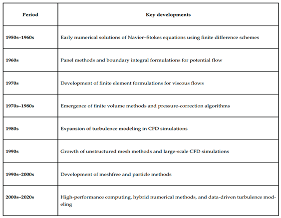
Table 2.
Comparison: BEM vs. FEM.
| Feature | Boundary Element Method (BEM) | Finite Element Method (FEM) |
|---|---|---|
| Mesh Requirements | Boundary only. Easy to mesh complex or changing shapes. | Full domain. Meshing complex 3D volumes is highly time-consuming. |
| Infinite Domains | Excellent. Inherently handles unbounded fields (e.g., acoustics, soil mechanics). | Poor. Requires artificial truncated boundaries or infinite elements. |
| Matrix Type | Fully dense and asymmetric. Expensive to solve for massive node counts. | Sparse and symmetric. Very fast to solve even with millions of elements. |
| Internal Accuracy | Extremely high. Calculated using exact analytical solutions. | Approximated. Dependent on the local polynomial element shapes. |
| Nonlinear Problems | Difficult. Requires volume integrals if materials yield or change properties. | Excellent. Naturally handles plasticity, large strains, and mixed materials. |
Table 3.
Comparative characteristics of principal numerical methods.
| Aspect | BEM | FDM | FEM | FVM | Meshfree / Meshless |
|---|---|---|---|---|---|
| Primary discretization | Boundary | Entire domain | Entire domain | Entire domain | Entire domain |
| Mathematical basis | Boundary integrals | Differential operators | Weak/variational | Integral conservation | Kernel/particle approximation |
| Nonlinearity | Limited | Strong | Strong | Strong | Strong |
| Turbulence | Limited | Excellent for canonical problems | Excellent | Excellent | Emerging |
| Infinite domains | Excellent | Limited | Moderate | Moderate | Moderate |
| Complex geometry | Good | Moderate | Excellent | Excellent | Excellent |
| Moving interfaces | Limited | Difficult | Good | Good | Excellent |
| Matrix structure | Dense | Sparse/structured | Sparse | Sparse | Sparse / Dense dependent |
| Industrial CFD | Specialized | Limited | Common | Dominant | Emerging |
Disclaimer/Publisher’s Note: The statements, opinions and data contained in all publications are solely those of the individual author(s) and contributor(s) and not of MDPI and/or the editor(s). MDPI and/or the editor(s) disclaim responsibility for any injury to people or property resulting from any ideas, methods, instructions or products referred to in the content. |
© 2026 by the authors. Licensee MDPI, Basel, Switzerland. This article is an open access article distributed under the terms and conditions of the Creative Commons Attribution (CC BY) license (http://creativecommons.org/licenses/by/4.0/).
Copyright: This open access article is published under a Creative Commons CC BY 4.0 license, which permit the free download, distribution, and reuse, provided that the author and preprint are cited in any reuse.