

Submitted:
12 August 2026
Posted:
13 August 2026
You are already at the latest version
Abstract
Listed-Rule Firewalls (LRF), deployed in iptables, nftables, Cisco ACL, and pfSense, suffer from linear matching complexity and structural anomalies affecting a large share of production rules. This paper presents an automated, formally proven framework converting LRF policies into Tree-Rule Firewall (TRF) structures. It combines a unified four-dimensional range decomposition, a projection normalization algorithm generalized to all twelve valid attribute orderings, and protocol-dependent destination-port semantics for ICMP. A tree is fixed by a permutation of the four packet attributes, so the admissible orderings form the half of the symmetric group S₄ placing protocol before dst_port. Three theorems and four propositions establish that this admissible set is exactly half the group and that the tree returns the same action as the original policy for every packet under every admissible ordering: semantics is invariant, structural cost is not. Evaluation on 10,000 synthetic policies (73 million packet comparisons) records no semantic discrepancy; on industry-calibrated synthetic ClassBench-ng rulesets, tree depth stays at its by-construction maximum of four with no early collapse. A 10,000-policy benchmark quantifies the broken cost symmetry: protocol-first orderings dominate at small sizes but reach statistical equivalence in matching time by 200 rules, while their structural advantage persists. All evaluated policies contain at most 400 rules.
Keywords:
permutation symmetry
; invariance under group action
; symmetry breaking
; Tree-Rule Firewall
; packet classification
; formal verification
; attribute ordering
1. Introduction
Network firewalls are the primary line of defense for modern network infrastructure, deciding which packets are permitted to cross a network boundary based on a declared access-control policy. The vast majority of deployed firewalls today implement the Listed-Rule Firewall (LRF) model: an ordered list of rules evaluated by first-match semantics. This model underlies iptables, nftables, Cisco ACLs, Juniper firewall filters, pfSense, and virtually every commercial and open-source firewall product.
Despite its ubiquity, the LRF model has two well-documented structural limitations:
Limitation L1 — O(n) matching complexity. Each incoming packet may need to be compared against all n rules before a match is found. In enterprise deployments with hundreds to thousands of rules, this linear scan becomes a throughput bottleneck.
Limitation L2 — Structural anomalies. Real-world firewall audits reveal Shadow, Redundancy, and Correlation anomalies in 50–80% of deployed rules [1,2]. These anomalies lead to silent policy errors, security gaps, and difficulty in policy maintenance.
The Tree-Rule Firewall (TRF) model proposed by Chomsiri, He, and Nanda [3] and developed in subsequent work [4,5,6,7,8,9] addresses L1 by organizing rules into a hierarchical decision tree that matches in O(d) where d ≤ 7 is a depth upper bound. However, prior TRF work assumed manual tree construction by experts; no automated LRF-to-TRF conversion algorithm existed, making practical migration of large LRF deployments infeasible.
This paper presents the first complete, formally proven, and experimentally validated framework for automated LRF-to-TRF conversion. The framework introduces a generalized Algorithm 1 supporting twelve attribute orderings, protocol-dependent dst_port semantics for ICMP, and a compiled Cython kernel executing the same O(d) traversal at native speed on industry-calibrated synthetic workloads.
1.1. Contributions
C1 — Algorithmic core. A six-step LRF-to-TRF conversion pipeline integrating (a) Unified 4D Range Decomposition for protocol/IP/port partitioning; (b) a generalized Projection Normalization (Algorithm 1) supporting twelve orderings in both per-protocol and global modes; and (c) protocol-dependent dst_port semantics with ICMP-type [0, 255] validation.
C2 — Deterministic anomaly detection. An exhaustive O(n²) Triad Classifier using exact integer arithmetic, detecting Shadow and Redundant anomalies with formal completeness proof (Proposition 2). Correlation anomalies are resolved implicitly by Stage 4 (Unified 4D Range Decomposition).
C3 — End-to-end formal correctness. Three theorems and Corollary 1 prove that φ_LRF(P, ψ) = φ_LRF(P′, ψ) = φ_TRF(T, ψ) for every packet ψ ∈ Ω, with validity established for all twelve orderings.
C4 — Evaluation on industry-calibrated synthetic ClassBench-ng rulesets. A controlled comparison of TRF against a Firewall Decision Diagram (FDD)-style fixed-order ablation [19] and HiCuts [16] on 8 ClassBench-ng rulesets (ACL, FW, IPC) at n ∈ {50, 100, 200, 400} rules. TRF depth stays at its by-construction maximum d = 4 across all 32 test cases (8 rulesets × 4 sizes); depth 4 is a design property of the four-attribute tree, and the experiments verify the absence of early collapse rather than discovering the constant empirically.
C5 — Compiled implementation and scale-aware ordering analysis. A Cython kernel achieving 40×–41× speedup (39× at n=25) over the pure-Python reference of the same TRF algorithm (a same-algorithm, different-runtime comparison), plus a 10,000-policy ordering-comparison benchmark across n ∈ {50, 100, 200, 400} documenting a previously unreported scaling phenomenon: protocol-first orderings (IDs 1–6) outperform protocol-elsewhere orderings (IDs 7–12) on all five metrics at n=50 with a perfect matched-pairs rank-biserial effect size (r=1.00), significant after Holm-Bonferroni correction across the full family of 20 comparisons (16 of 20 comparisons survive correction); the timing advantage shrinks monotonically and reaches confirmed statistical equivalence (TOST) at n=200 (untested at n=400), while structural metrics (tree memory, node count, and peak memory, verified via tracemalloc) remain significant across all sizes.
The paper is structured as follows. Section 1.2 sets out the symmetry framing that organizes the results. Section 2 reviews related work. Section 3 defines the formal model. Section 4 describes the conversion pipeline. Section 5 presents the proofs. Section 6 reports experimental evaluation including ClassBench-ng benchmarks and the Cython implementation. Section 7 discusses design rationale. Section 8 presents threats to validity. Section 9 concludes.
Novelty positioning. To situate these contributions, we distinguish adopted foundations from novel elements. The framework builds on established components — the Shadow/Redundancy/Correlation anomaly taxonomy [1,2], geometric decision-tree decomposition for packet classification [16,19], and O(d) tree traversal — which we adopt rather than claim as new. The novelty lies in their integration and extension: (i) the first fully automated, formally verified LRF-to-TRF conversion whose end-to-end correctness (Corollary 1) is established by formal proofs, with an independent Z3-SMT oracle machine-checking the pairwise-containment decisions of the anomaly classifier (Section 6.1); (ii) the generalization of Projection Normalization (Algorithm 1) to all twelve attribute orderings in per-protocol and global modes, versus the single fixed ordering of FDD; (iii) scale-aware ordering selection derived from the crossover analysis; and (iv) protocol-dependent dst_port semantics (Definition 1.bis) enabling ICMP-aware decomposition. To our knowledge, no prior TRF work provides automated construction with formally proven correctness, and no prior packet-classification tree offers this ordering generality.
1.2. Symmetry Perspective
The framework is organized around a symmetry of the packet space. A Tree-Rule Firewall assigns one attribute to each level of the tree, so a tree is determined by a permutation of the four attributes {protocol, src_ip, dst_ip, dst_port}. These permutations form the symmetric group S₄ of order 24, acting on the set of admissible tree shapes. The protocol-dependent semantics of dst_port (Definition 1.bis) breaks this action: a permutation is admissible only when protocol precedes dst_port, which selects exactly half of the group, the twelve orderings enumerated in Table 1. The admissible set is thus exactly half of S₄ — Proposition 3 proves this by exhibiting an involution that pairs each admissible ordering with an inadmissible one — so the number twelve is a consequence of that single constraint rather than an arbitrary design choice.
Two results follow, and they pull in opposite directions. First, the semantics of the firewall is invariant under this action: Corollary 1 states that φ_TRF(Tₐ, ψ) = φ_LRF(P, ψ) for every packet ψ and every admissible ordering a, and Theorem 3 restates this as constancy on the whole set: all twelve trees, however different their shapes, are indistinguishable as functions on the packet space. The accept/deny decision is a group invariant. Second, the structural cost of the tree is not invariant: Proposition 4 records this formally, and node count, memory, and construction time differ systematically between the protocol-first and protocol-elsewhere sub-families (Section 6.5, Table 3) at every tested policy size. The group therefore acts freely on structure while fixing semantics — a partial symmetry breaking in which an exact functional symmetry coexists with a broken cost symmetry.
This is what makes the ordering question well-posed. Because semantics is invariant, an implementer may choose any of the twelve orderings without changing the firewall's behavior, and is free to choose on cost grounds alone; because cost is not invariant, that choice matters. The scale-aware finding of Section 6.5 — that the protocol-first advantage in timing decays with policy size and reaches statistical equivalence by n=200, while the structural advantage persists at all sizes — is a statement about how far the cost symmetry is broken as a function of scale. The decomposition itself has a related structure: Projection Normalization operates independently on each protocol class in per-protocol mode, so the packet space factors into protocol-indexed subspaces that are treated symmetrically and recombined without interaction (Lemma 1.A).
2. Related Work
2.1. Firewall Anomaly Detection
The foundational taxonomy of firewall rule anomalies was established by Al-Shaer and Hamed [1], who identified Shadowing, Correlation, Redundancy, Generalization, and Irrelevance, and developed the Firewall Policy Advisor (FPA) using pairwise rule comparisons. The containment conditions formalized in [1] are the conceptual ancestor of conditions (C1)–(C4) in our Deterministic Triad. Al-Shaer et al. [2] extended the framework to distributed firewall conflict classification.
Hamed and Al-Shaer [10] studied dynamic rule ordering. Yuan et al. [11] developed FIREMAN with BDD-based symbolic model checking. Marmorstein and Kearns [12] built an iptables analyzer. Abedin et al. [13] proposed dependency-graph approaches. Hu et al. [14] used formal policy models. Mayer et al. [15] developed FANG for offline analysis. None of these works provide automated structural conversion to TRF with end-to-end formal correctness guarantees.
2.2. The Tree-Rule Firewall Research Programme
The TRF research line, initiated by Chomsiri, He, and Nanda [3], formalized five LRF limitations on large-scale networks. He et al. [4] extended TRF to cloud network security. Chomsiri et al. [5] added stateful packet classification. The work [6] studied scalability, and [7] presented Hybrid TRF. Chomsiri's PhD thesis [8] provides the most comprehensive formal analysis of TRF. The present work delivers the first automated LRF-to-TRF conversion with end-to-end correctness guarantees and the first empirical comparison against an FDD-style fixed-order ablation and HiCuts on industry-calibrated synthetic ClassBench-ng rulesets.
2.3. Packet Classification Algorithms
Gupta and McKeown [16] surveyed multi-dimensional packet classification and proposed HiCuts (Hierarchical Intelligent Cuttings), a decision-tree approach with linear-scan leaves. Srinivasan et al. [17] proposed tuple space search. Taylor and Turner [18] introduced ClassBench, the established synthetic ruleset benchmark. Liu and Gouda [19] proposed Firewall Decision Diagrams (FDD), which share TRF's O(d) matching property but are limited to a single fixed attribute ordering. Liu et al. [20] developed TCAM Razor. Bartal et al. [21] developed Firmato. Jeffrey and Samak [22] applied model checking to firewall policy verification. Garcia-Alfaro, Cuppens, and Cuppens-Boulahia [23] analyzed policy anomalies across distributed setups combining firewalls and network intrusion detection systems. Cormen et al. [24] provide the algorithmic foundations for sweep-line algorithms used in Stage 4 (4D Decomposition). Liu and Gouda [25] addressed complete redundancy detection in firewalls. Recent work includes NeuroCuts [26] (deep RL for cut selection, SIGCOMM 2019) and ClassBench-ng [27] (an updated generator).
The present work supports twelve configurable orderings (versus FDD's single ordering), provides the first empirical comparison, and is the first TRF work evaluated alongside an FDD-style fixed-order ablation and HiCuts on the same ClassBench-ng datasets.
Broader packet-classification and verification context. Beyond HiCuts [16], a family of cut-based decision-tree classifiers has advanced the memory–throughput trade-off: HyperCuts [29] cuts on multiple dimensions per node, EffiCuts [30] separates rules by field range size to curb replication, and CutSplit [31] adaptively combines cutting and splitting; learning-based partitioning such as NeuroCuts [26] applies deep reinforcement learning to cut selection. These methods optimize average memory and speed but build trees whose depth is variable and data-dependent — precisely the property our comparison probes: TRF maintains a constant depth d = 4 (bounded d ≤ 7) across all tested rulesets, whereas HiCuts depth ranges from 1 to 12 across the same 32 cases. On the verification side, general network-property checkers such as Header Space Analysis [32] statically analyze reachability and isolation across protocols; our work is complementary and narrower, providing a formally proven equivalence between a specific LRF policy and its constructed TRF (with SMT machine-checking of the anomaly classifier's pairwise-containment decisions) rather than network-wide reachability analysis.
3. Formal Model
3.1. Basic Definitions
All IPv4 addresses are represented as unsigned 32-bit integers in [0, 2³²−1]. Port numbers are unsigned 16-bit integers in [0, 65535]. CIDR notation X.X.X.X/n is interpreted as a closed integer range [network_address, broadcast_address]. The notation [a, b] denotes a closed integer range.
Definition 1 (LRF Rule). An LRF rule is a 5-tuple r = ⟨π, σ, δ, ρ, α⟩ where π ∈ {IP, TCP, UDP, ICMP, ANY} is the protocol identifier; σ = [σ_s, σ_e] ⊆ [0, 2³²−1] is the source IP range (closed integer interval); δ = [δ_s, δ_e] ⊆ [0, 2³²−1] is the destination IP range; ρ = [ρ_s, ρ_e] is the destination port range (domain determined by π per Definition 1.bis); and α ∈ {ALLOW, DENY} is the action.
Definition 1.bis (Domain of ρ). The destination-port range ρ has a protocol-dependent domain: ρ ∈ [0, 65535] when π ∈ {TCP, UDP, IP, ANY}; and ρ ∈ [0, 255] when π = ICMP. In the ICMP case, ρ stores the ICMP type (per RFC 792 / 4884), which is an 8-bit field. Out-of-range values are rejected during parsing. Figure 1 contrasts the two domains.
Definition 2 (Protocol Containment Function Π). Π maps protocol identifiers to sets of atomic protocols: Π(TCP) = {TCP}, Π(UDP) = {UDP}, Π(ICMP) = {ICMP}, Π(IP) = Π(ANY) = {TCP, UDP, ICMP}. (Modeling assumption: the framework supports the three atomic protocols {TCP, UDP, ICMP}. IP and ANY are treated as super-sets of these three; other IP protocol numbers such as GRE (47) or ESP (50) are outside the scope of this model and would require extending the framework.)
Definition 3 (Match Space). The match space of rule r is M(r) = {ψ = (π_ψ, σ_ψ, δ_ψ, ρ_ψ) : π_ψ ∈ Π(π), σ_s ≤ σ_ψ ≤ σ_e, δ_s ≤ δ_ψ ≤ δ_e, ρ_s ≤ ρ_ψ ≤ ρ_e}. Note that ρ_ψ is compared within the protocol-appropriate domain: for π_ψ ∈ {TCP, UDP}, ρ_ψ ∈ [0, 65535]; for π_ψ = ICMP, ρ_ψ ∈ [0, 255] (Definition 1.bis). Equivalently, M(r) ⊆ Π(π) × σ × δ × ρ where σ = [σ_s, σ_e], δ = [δ_s, δ_e], ρ = [ρ_s, ρ_e] ∩ dom(π). The complete packet space is Ω = ⋃_{p ∈ {TCP,UDP,ICMP}} ({p} × [0, 2³²−1] × [0, 2³²−1] × dom(p)), where dom(TCP) = dom(UDP) = [0, 65535] and dom(ICMP) = [0, 255].
Definition 4 (LRF Policy). An LRF policy P = ⟨r₁, …, r_n⟩ is an ordered list. The policy function φ_LRF(P, ψ) = α_k where k = min{i : ψ ∈ M(r_i)} returns the action of the first matching rule, with implicit DENY default.
Definition 5 (Structural Anomaly Types). Given r_i, r_j ∈ P with i < j: Shadow: M(r_j) ⊆ M(r_i) and α_i ≠ α_j. Redundancy: M(r_j) ⊆ M(r_i) and α_i = α_j. Correlation: M(r_i) ∩ M(r_j) ≠ ∅ and neither contains the other.
Definition 6 (Tree-Rule Firewall). A TRF is a rooted, labeled tree T such that: (i) each internal node carries an attribute label from an ordering A* = ⟨a₁, a₂, a₃, a₄⟩ which is a permutation of {protocol, src_ip, dst_ip, dst_port}; (ii) each edge carries a value range, with sibling edge ranges disjoint; (iii) each leaf carries an action; and (iv) T is complete: the union of all root-to-leaf paths covers Ω, so every packet ψ ∈ Ω reaches exactly one leaf (guaranteed by the deny-all rule appended in Stage 1 and Lemma 2).
3.2. The Twelve Valid Attribute Orderings
The permutation space of four attributes contains 4! = 24 orderings. The sole semantic constraint is that protocol must precede dst_port (because the domain of dst_port depends on the protocol; Def. 1.bis). In any permutation of four elements, each pair occupies exactly one of two relative orders; hence exactly 24/2 = 12 permutations have protocol before dst_port, and 12 have dst_port before protocol. In the language of Section 1.2, the constraint selects one half of the symmetric group S₄ acting on the attribute set, and the transposition that swaps protocol with dst_port maps the admissible half onto the inadmissible one. The 12 valid orderings are enumerated in Table 1. Theorem 1 holds for all twelve. Orderings 1–6 (protocol at position 1) are called protocol-first (PF); orderings 7–12 are protocol-elsewhere (PE).
4. LRF-to-TRF Conversion Framework
4.1. Pipeline Architecture
The framework converts an LRF policy P into a TRF T in six sequential stages, each with explicit pre/post-conditions and time complexity. Together, the six stages implement Corollary 1: φ_LRF(P, ψ) = φ_TRF(T, ψ) for every packet ψ ∈ Ω. Figure 2 shows the pipeline.
The six stages are:
Stage 1 — Parsing and Deny-All Normalization. Parses rules with two validity checks: (i) for π ∈ {TCP, UDP, IP, ANY}, requires 0 ≤ ρ_s ≤ ρ_e ≤ 65535; (ii) for π = ICMP, requires 0 ≤ ρ_s ≤ ρ_e ≤ 255 (Def. 1.bis). If the last rule is not deny-all, it is appended automatically.
Stage 2 — Anomaly Detection (Deterministic Triad). Performs O(n²) exhaustive verification on all n(n−1)/2 rule pairs, removing detected Shadow and Redundant rules to yield a conflict-free policy P′. Proposition 1 proves this removal preserves semantics.
Stage 3 — Attribute Ordering Selection. The administrator selects one of twelve orderings; the default is Ordering 4. The selected A* governs Stages 4–5.
Stage 4 — Unified 4D Range Decomposition. Partitions Ω into disjoint, exhaustive cells via a 4D decomposition. The sweep-line phase is protocol-aware: dst_port axis bounds are 256 for ICMP atoms and 65,536 for TCP/UDP atoms.
Stage 5 — Projection Normalization (Algorithm 1). Algorithm 1 re-cuts cells along each non-protocol attribute axis to eliminate inter-group overlap. Two modes (per-protocol and global) uniformly handle all twelve orderings.
Stage 6 — TRF Construction. Normalized cells are hierarchically grouped following A*. By Proposition 1 and Corollary 1, the resulting tree T returns identical decisions to the original policy P for every packet in Ω: φ_LRF(P, ψ) = φ_LRF(P′, ψ) = φ_TRF(T, ψ).
4.2. Anomaly Type Visualization
The Deterministic Triad in Stage 2 classifies every rule pair using the containment conditions (C1)–(C4). Shadow anomalies arise when one rule completely masks another with a conflicting action; Redundancy when the action is identical; and Correlation when neither rule completely contains the other but their match spaces overlap. Figure 3 shows the three types in a two-dimensional projection of the match space.
4.3. Protocol Hierarchy Expansion
Phase 1 of the 4D Decomposition resolves the protocol hierarchy before any spatial decomposition. The IP and ANY identifiers are super-sets of the three atomic protocols. Protocol expansion replicates rules into atom-specific sub-rules, after which first-match is applied independently per atom. For ICMP sub-rules, the dst_port range is clipped to [0, 255] per Definition 1.bis. Figure 4 illustrates this expansion.
4.4. Unified 4D Range Decomposition
The 4D Decomposition operates in four phases: (1) protocol expansion (Section 4.3); (2) cell construction via 3D sweep-line with protocol-aware axis bounds; (3) action assignment to each cell from the highest-priority matching rule; (4) merging of adjacent cells with identical actions. Figure 5 summarizes the four phases.
Complexity. Let n = |P′| and N = O(n³) be the maximum number of cells after Phase 2. Phase 1: O(n). Phase 2: O(N·n). Phase 3: O(N log N). Stage 5 (Projection Normalization): O(N²) worst case. The O(N²) normalization is the dominant cost at large n, as confirmed empirically in Figure 6.
4.5. Algorithm 1: Projection Normalization (Generalized)
| Algorithm 1: Projection Normalization (Generalized) |
| Input: cells C, ordering A* = 〈a1, a2, a3, a4〉 Output: normalized cells C′ satisfying Disjointness Invariant 1: for j = 2 to 4 do 2: a_j ← A*[j] 3: if ‘protocol’ appears at position k > j in A* then // global mode 4: G ← collect_cut_points(C, a_j) 5: C ← re_cut_against(C, a_j, G) 6: else // per-protocol mode 7: for each p ∈ {TCP, UDP, ICMP} do 8: C_p ← cells_with_protocol(C, p) 9: ρ̃ ← 256 if p=ICMP else 65,536 10: L_p ← collect_cut_points(C_p, a_j, max=ρ̃) 11: C ← (C \ C_p) ∪ re_cut_against(C_p, a_j, L_p) 12: end for 13: end if 14: end for 15: return C |
Figure 7 contrasts a fragment of the tree before and after normalization: sibling ranges that overlap beforehand become disjoint afterwards, so every packet reaches exactly one leaf.
Lines 4–5 (global mode) execute only for orderings with protocol at level 2, 3, or 4 (IDs 7–12). For orderings 1–6 (protocol at level 1), only the per-protocol branch (lines 7–12) executes. Lemma 1.A (G_j ⊇ ⋃_p L_{p,j}) establishes that global mode is at least as fine-grained as the union of per-protocol modes.
4.6. Deterministic Triad Classifier
The Deterministic Triad performs an exhaustive O(n²) verification on all n(n−1)/2 rule pairs. For each pair (r_i, r_j) with i < j, four conditions test whether M(r_j) ⊆ M(r_i):
(C1) Π(π_j) ⊆ Π(π_i) [protocol containment]
(C2) σ_s(r_i) ≤ σ_s(r_j) ∧ σ_e(r_j) ≤ σ_e(r_i) [Src-IP containment]
(C3) δ_s(r_i) ≤ δ_s(r_j) ∧ δ_e(r_j) ≤ δ_e(r_i) [Dst-IP containment]
(C4) ρ_s(r_i) ≤ ρ_s(r_j) ∧ ρ_e(r_j) ≤ ρ_e(r_i) [Dst-Port containment]
Conditions (C1)–(C4) jointly form a necessary and sufficient condition for M(r_j) ⊆ M(r_i) (Lemma 4 in Section 5.4). All comparisons use exact integer arithmetic; no approximation, sampling, or floating-point computation is involved.
5. Formal Analysis
This section presents the correctness proofs. The dependency structure: Lemmas 1–3 support Theorem 1; Theorem 2 follows from Lemma 1; Lemma 4 supports Proposition 2; Corollary 1 combines Proposition 1 and Theorem 1. Figure 8 shows this dependency chain.
5.1. Proposition 1 — Anomaly Removal Preserves Semantics
Proposition 1. Let P′ = P ∖ {r_j : r_j is Shadow or Redundant in P}. Then for every packet ψ: φ_LRF(P, ψ) = φ_LRF(P′, ψ).
Proof sketch. By case analysis on every rule r_j removed from P. Case 1 — r_j is Redundant: there exists r_i with i < j and M(r_j) ⊆ M(r_i) and α_i = α_j. For any ψ ∈ M(r_j), rule r_i matches ψ before r_j (since i < j), so φ_LRF(P, ψ) = α_i. After removing r_j, r_i still matches ψ first, giving φ_LRF(P′, ψ) = α_i = α_j. Hence φ_LRF(P, ψ) = φ_LRF(P′, ψ). Case 2 — r_j is Shadow: there exists r_i with i < j and M(r_j) ⊆ M(r_i) and α_i ≠ α_j. For any ψ ∈ M(r_j), r_i matches ψ before r_j in P (since i < j and M(r_j) ⊆ M(r_i)), so φ_LRF(P, ψ) = α_i. After removing r_j from P, r_i still matches ψ first, so φ_LRF(P′, ψ) = α_i. Hence φ_LRF(P, ψ) = φ_LRF(P′, ψ). For ψ ∉ ⋃_j M(r_j) (packets not covered by any removed rule), the first-match rule is unchanged in both P and P′. Note that removing a rule from P cannot create new Shadow or Redundant anomalies: removal can only reduce containment relationships, never introduce new ones. Therefore the anomaly classification of remaining rules is preserved across the removal sequence, and the induction invariant holds. By induction on the removal sequence, the claim holds for all removals. □
5.2. Theorem 1 — Semantic Preservation
Theorem 1. Let P′ be conflict-free and T = BuildTRF(P′, A*) where A* is any of the twelve valid orderings. Then for every ψ ∈ Ω: φ_LRF(P′, ψ) = φ_TRF(T, ψ).
Lemma 1.A (Global Cut Coverage). Let G_j be the global cut-point set on axis a_j computed in line 4 of Algorithm 1, and L_{p,j} the per-protocol cut-point set computed in line 10 for atomic protocol p. Then G_j ⊇ ⋃_p L_{p,j} for p ∈ {TCP, UDP, ICMP}.
Proof of Lemma 1.A. By construction, collect_cut_points(C, a_j) traverses every cell c ∈ C and adds both endpoints (lo_j(c), hi_j(c)+1) to G_j. The set L_{p,j} = collect_cut_points(C_p, a_j) operates only on the subset C_p = {c ∈ C : protocol(c) = p}, so its cut-points are a subset of those collected from C. Since C = ⋃_p C_p (cells are partitioned by protocol after Phase 1), the union ⋃_p L_{p,j} ⊆ G_j. □
Lemma 1 (Disjointness After Normalization). After Algorithm 1 terminates, the cell set C is pairwise non-overlapping, regardless of which of the twelve orderings is used.
Proof of Lemma 1. By induction on j ∈ {2, 3, 4} (the axes normalised by Algorithm 1; axis a₁ is handled by the sweep-line in Stage 4 which produces non-overlapping ranges on a₁ by construction). Base case (j = 2): after Stage 4 the cells are non-overlapping on a₁; Algorithm 1 re-cuts on axis a₂ using a shared cut-point set (per-protocol L_{p,2} or global G₂), subdividing cells without introducing new overlaps on a₁ and making sibling edge-ranges on a₂ disjoint: re-cutting against a sorted cut-point set partitions any interval into disjoint sub-intervals covering the original (standard interval-partitioning property [24, Ch. 33]). Inductive step (j → j+1): assuming non-overlap on prefix ⟨a₁, …, a_j⟩, Algorithm 1 re-cuts on a_{j+1}: in per-protocol mode, re-cutting against L_{p,j+1} preserves non-overlap within each protocol subtree; in global mode, re-cutting against G_{j+1} ⊇ ⋃_p L_{p,j+1} (Lemma 1.A) preserves non-overlap across all protocols simultaneously. □
Lemma 2 (Completeness). The cell set C covers Ω: every packet ψ ∈ Ω lies in at least one cell. Proof. Stage 1 appends a deny-all rule r_∞ = ⟨ANY, [0,2³²−1], [0,2³²−1], [0, 65535], DENY⟩. After Protocol Expansion (Stage 4, Phase 1), r_∞ is replicated into three atom-specific rules covering {TCP} × [0,2³²−1] × [0,2³²−1] × [0, 65535], {UDP} × [0,2³²−1] × [0,2³²−1] × [0, 65535], and {ICMP} × [0,2³²−1] × [0,2³²−1] × [0, 255], whose union equals Ω (using the protocol-aware domains from Definition 1.bis). The sweep-line in Phase 2 inserts cut-points including 0 and ρ̃_max = {65535 for TCP/UDP, 255 for ICMP} on each protocol-specific axis, guaranteeing that every ψ ∈ Ω is covered by at least one cell derived from the r_∞ replicas. Hence C tiles Ω. □
Lemma 3 (First-Match Consistency). For every cell c_k ∈ C and every packet ψ ∈ c_k: action(c_k) = φ_LRF(P′, ψ). Proof. The 4D Decomposition (Stage 4) assigns to each cell c_k the action action(c_k) = α_{i*} where i* = min{t : c_k ⊆ M(r_t), r_t ∈ P′} — i.e., the action of the lowest-indexed rule in P′ whose match space contains c_k. We show action(c_k) = φ_LRF(P′, ψ) for every ψ ∈ c_k. Let i = min{t : ψ ∈ M(r_t)} (the first-match index for ψ in P′). We claim i = i*. (i ≤ i*): since ψ ∈ c_k ⊆ M(r_{i*}), rule r_{i*} covers ψ, and i is the least such index, so i ≤ i*. (i* ≤ i): suppose for contradiction that i < i*. Then ψ ∈ M(r_i), so r_i covers ψ. Since cells are pairwise non-overlapping (Lemma 1) and ψ ∈ c_k, cell c_k is the unique cell containing ψ. Because ψ ∈ c_k ∩ M(r_i), we have c_k ∩ M(r_i) ≠ ∅. The 4D Decomposition creates cells as intersections of rule ranges along every axis. The 4D Decomposition inserts cut-points at every endpoint of every rule range on every axis; therefore each cell lies entirely within or entirely outside each rule's match space (it cannot straddle a rule boundary). Formally: since ψ ∈ c_k ∩ M(r_i) ≠ ∅, we have c_k ⊆ M(r_i). But i < i*, contradicting the minimality of i*. Hence i = i*, so action(c_k) = α_{i*} = α_i = φ_LRF(P′, ψ). □
Proof of Theorem 1. From Lemmas 1+2, every ψ lies in exactly one cell c_k. From Lemma 3, action(c_k) = φ_LRF(P′, ψ). BuildTRF groups cells according to A*; by Lemma 1, edge ranges at every level are non-overlapping, so tree traversal for any ψ follows a unique root-to-leaf path returning action(c_k) = φ_LRF(P′, ψ). □
Corollary 1 (End-to-End Correctness). For any LRF policy P and T = BuildTRF(P′, A*) where P′ is the conflict-free policy from Stage 2: φ_LRF(P, ψ) = φ_LRF(P′, ψ) = φ_TRF(T, ψ) for every ψ ∈ Ω. □
Restated in the terms of Section 1.2: φ_TRF is constant on the admissible orderings; Theorem 3 in Section 5.5 states this consequence formally. The twelve trees are distinct objects with different node counts and memory footprints, yet they induce the same function on the packet space Ω, so the firewall's semantics is an invariant of the group action while its structure is not.
5.3. Theorem 2 — Disjointness Invariant
Theorem 2. Let {l₁, …, l_K} be the leaves of T = BuildTRF(P′, A*), and let M(l_i) denote the set of packets that reach leaf l_i (i.e., the packet space covered by the root-to-l_i path). For every pair of distinct leaves l_i ≠ l_j: M(l_i) ∩ M(l_j) = ∅. Proof. Stage 4 performs cell merging (Phase 4) before BuildTRF is called, combining adjacent cells with identical actions. BuildTRF (Stage 6) then creates exactly one leaf per post-merge cell by hierarchically grouping cells along A* without further merging, so each leaf l_i corresponds to exactly one post-merge cell c_i. By Lemma 1, these cells are pairwise non-overlapping, so M(l_i) = c_i and M(l_i) ∩ M(l_j) = c_i ∩ c_j = ∅ for i ≠ j. □ Figure 9 shows the resulting tree anatomy: one attribute per level, with disjoint edge ranges at every node.
5.4. Proposition 2 — Detection Completeness
Lemma 4 (Containment Equivalence). M(r_j) ⊆ M(r_i) if and only if conditions (C1)–(C4) all hold.
Proof of Lemma 4. (⟸) Assume (C1)–(C4). Pick any ψ = (π, σ, δ, ρ) ∈ M(r_j). Then π ∈ Π(π_j), and Π(π_j) ⊆ Π(π_i) by (C1), so π ∈ Π(π_i). IP/port containment follows from (C2)–(C4): σ_s(r_i) ≤ σ_s(r_j) ≤ σ ≤ σ_e(r_j) ≤ σ_e(r_i), and similarly for δ and ρ. So ψ ∈ M(r_i), hence M(r_j) ⊆ M(r_i). (⟹) Assume M(r_j) ⊆ M(r_i) but (C1) fails. Then there exists an atomic p ∈ Π(π_j) ∖ Π(π_i). Since Stage 1 validates ρ_s ≤ ρ_e, σ_s ≤ σ_e, δ_s ≤ δ_e for every rule, M(r_j) ≠ ∅. Constructing ψ with π = p and any (σ, δ, ρ) ∈ σ_j × δ_j × ρ_j gives ψ ∈ M(r_j) but ψ ∉ M(r_i) (since p ∉ Π(π_i)), contradicting M(r_j) ⊆ M(r_i). The same construction handles (C2)–(C4): if C2 fails then σ_s(r_j) < σ_s(r_i) or σ_e(r_j) > σ_e(r_i); choose σ = σ_s(r_j) (resp. σ_e(r_j)) and valid π,δ,ρ to obtain ψ ∈ M(r_j) \ M(r_i). Cases (C3), (C4) are symmetric. □
Proposition 2 (Detection Completeness). The Deterministic Triad flags every Shadow and Redundant rule as defined pairwise in Definition 5. Equivalently, Recall = TP / (TP + FN) = 1.0 by construction, where TP denotes true positives and FN false negatives.
Proof. Suppose r_j is anomalous (Shadow or Redundant) but unflagged. Then there exists r_i with i < j such that M(r_j) ⊆ M(r_i). By Lemma 4, conditions (C1)–(C4) all hold. The Triad exhaustively checks all n(n−1)/2 ordered pairs using exact integer arithmetic. For pair (r_i, r_j), the four conditions are all true, so the Triad flags r_j — contradicting the assumption. □
Precision = 100% follows directly from Lemma 4: conditions (C1)–(C4) are both necessary and sufficient, so flagged pairs must satisfy M(r_j) ⊆ M(r_i).
5.5. Symmetry Properties of the Admissible Ordering Set
The results above establish correctness for a fixed ordering. This section states what the framework guarantees across orderings, in the group-theoretic terms introduced in Section 1.2. Write A for the set of admissible orderings, that is, the permutations of the four attributes in which protocol precedes dst_port, and write T_a = BuildTRF(P′, a) for the tree built from the conflict-free policy P′ under ordering a ∈ A.
Proposition 3 (Cardinality of the admissible set). |A| = 12; equivalently, the admissibility constraint selects exactly half of S₄.
Proof. Let t denote the transposition of the two attributes protocol and dst_port, and let τ(a) = t ∘ a; concretely, τ exchanges the positions occupied by protocol and dst_port in the ordering a, leaving the other two attributes in place. Then τ is well defined on all of S₄, since every ordering places protocol and dst_port at two distinct positions. It is an involution: applying it twice restores the original ordering, so ττ = id. It has no fixed point, because τ reverses the relative order of protocol and dst_port and no ordering can have protocol both before and after dst_port. Consequently τ is a bijection from A onto its complement in S₄: if a ∈ A then protocol precedes dst_port in a, so it follows dst_port in τ(a), and conversely. A bijection between a set and its complement forces the two to have equal size, hence |A| = |S₄|/2 = 24/2 = 12. The twelve members are enumerated in Table 1. □
The count is therefore not an empirical observation but a consequence of a single semantic constraint, the protocol-dependent domain of dst_port (Definition 1.bis). Note that A is not a subgroup of S₄. Identifying an ordering with the permutation that sends each position to the attribute tested there, composition of two admissible orderings need not be admissible: composing ⟨protocol, src_ip, dst_port, dst_ip⟩ with ⟨src_ip, dst_ip, protocol, dst_port⟩ yields ⟨src_ip, dst_port, protocol, dst_ip⟩, in which dst_port precedes protocol. A is instead one of the two blocks into which the involution τ partitions the group.
Theorem 3 (Semantic invariance under the group action). Let P be an LRF policy, P′ its conflict-free form, and T_a, T_a′ the trees built from P′ under two admissible orderings. For every pair a, a′ ∈ A and every packet ψ ∈ Ω: φ_TRF(T_a, ψ) = φ_TRF(T_a′, ψ). That is, φ_TRF is constant on A.
Proof. Corollary 1 holds for an arbitrary admissible ordering: for any a ∈ A, φ_TRF(T_a, ψ) = φ_LRF(P, ψ) for every ψ ∈ Ω. Fix ψ and apply this to a and to a′ separately; both sides equal φ_LRF(P, ψ), hence they are equal to each other. Since ψ was arbitrary, the two trees induce the same function on Ω. □
The twelve trees are distinct objects — they differ in shape, in node count, and in which attribute is tested at the root — yet Theorem 3 says they are indistinguishable as classifiers. The accept/deny behavior of the firewall is an invariant of the ordering choice, which is what licenses an implementer to select an ordering on cost grounds alone.
Proposition 4 (Non-invariance of structural cost). The structural cost of T_a is not constant on A. Specifically, there exist a, a′ ∈ A and a policy P such that the node counts of T_a and T_a′ differ.
Proof. A single counterexample suffices. Section 6.5 measures node count for the protocol-first family (orderings 1–6) against the protocol-elsewhere family (orderings 7–12) on the 10,000-policy dataset. At n = 50 the mean node count of the latter exceeds that of the former by a factor of 1.93 (Table 3), a difference significant under Holm-Bonferroni correction with a perfect matched-pairs rank-biserial effect size. Since the two family means differ, at least one ordering pair and one policy must realize that difference, which is all the claim requires. □
Theorem 3 and Proposition 4 together characterize the situation as a partial symmetry: the action of the admissible orderings fixes the semantics exactly while moving the structure. The experiments of Section 6 are best read as measurements of how far the cost symmetry is broken, and Section 6.5 shows that the extent of the breaking is itself scale-dependent — pronounced at small policy sizes in every metric, and confined to structural metrics once timing reaches statistical equivalence at n = 200.
6. Experimental Evaluation
6.1. Setup, Dataset, and Independent Oracle
All experiments were performed on a Windows 11 Home Single Language workstation (Intel Core 5 210H, 2.20 GHz; 32 GB DDR4 RAM) running Python 3.12.10. The implementation uses only the Python standard library; the Cython kernel in Section 6.8 requires Cython 3.x and a C99 compiler. Full source code is available at the GitHub repository (https://github.com/thawatchai2799/TreeRuleFirewall_20260526_2001) and archived at Zenodo [28].
Independent Oracle. To address potential circularity (the Triad and any verifier sharing the same containment conditions), we implemented an independent Z3-SMT oracle: each rule pair (r_i, r_j) is encoded as first-order logic over bit-vectors (32-bit IPs, 16-bit ports, 3-bit protocol enum), and Z3 checks (∀ψ: ψ ∈ M(r_j) ⟹ ψ ∈ M(r_i)). The Z3 implementation has a structurally distinct architecture from the algorithmic Triad, eliminating circularity concerns.
Honest interpretation of "100%". Reporting Recall = 100% on a finite test set is strictly an upper bound on the error rate. With 73,120,887 packet evaluations (Section 6.2) and zero failures, the Rule of Three [33] yields a 95% upper-CI on the FN rate of approximately 4.10×10⁻⁸. In this paper, "100%" on empirical data should be read as "failure rate ≤ 4.10×10⁻⁸ at 95% confidence," while "100%" on Proposition 2 is a deductive guarantee.
Synthetic dataset. 10,000 LRF policies stratified into three size categories: Small (1–25 rules), Medium (26–100 rules), and Large (101–400 rules). Protocol weights: TCP=40%, UDP=25%, ICMP=10%, IP=10%, ANY=15%. Each policy receives 0–5 controlled anomaly injections.
Real-world dataset. We use 8 ClassBench-ng [27] rulesets distributed by the NeuroCuts project [26]: ACL1, ACL2, ACL3 (access control), FW1, FW2, FW3 (firewall), IPC1, IPC2 (IP chain). For each, we sample n ∈ {50, 100, 200, 400} rules to enable controlled comparison with the FDD-style ablation and HiCuts within available compute budgets.
6.2. Verification Step 1 — Semantic Fidelity
We compared φ_LRF(P′, ψ) and φ_TRF(T, ψ) for every packet in two complementary test sets covering all 10,000 policies. The first is a uniform random set: 5,000 packets per policy, each field drawn uniformly from its domain (source and destination IP over [0, 2³²−1], dst_port over [0, 65535] for TCP/UDP and [0, 255] for ICMP, per Definition 1.bis), giving 50,000,000 evaluations. The second is a boundary set constructed per policy from the rule endpoints themselves: for every rule and every protocol it expands to, packets are emitted at each range start, each range end, the midpoint of the source range, and at start−1 and end+1 on both the source-IP and dst_port axes, clamped to the protocol-appropriate domain. This targets exactly the cut-points at which Projection Normalization splits cells, and the ±1 neighbours where an off-by-one error in the decomposition would surface; it contributes 23,120,887 evaluations, a mean of 2,312 per policy. Random sampling alone would place almost no probability mass on these points, so the boundary set, rather than the random set, is what stresses the correctness of the decomposition. The evaluation ran for approximately 10.7 hours and produced 73,120,887 packet-action comparisons with zero discrepancies (Table 2).
6.3. Verification Step 2 — Anomaly Detection
The Deterministic Triad was tested across 14 configurations (7 anomaly types × 2 size categories: Small 1–25, Medium 26–100) with 500 trials each, totaling 7,000 trials. Large policies (101+ rules) were excluded from this benchmark because the controlled-injection generator was calibrated for the Small/Medium range; anomaly detection correctness for all sizes is guaranteed by Proposition 2 and confirmed via the semantic fidelity benchmark (Section 6.2, all 10,000 policies). Each trial injects one or more anomalies per policy (configurations such as Normal (2S+2R) and Heavy (3S+2R) inject 4–5 anomalies per trial), yielding 20,868 total detected anomaly instances (TP) across all trials. Independent verification was performed by the Z3-SMT oracle on a 10% sample; the Triad and Z3 agreed on 100% of cases. Figure 10 reports the per-configuration counts.
6.4. Verification Step 3 — Scalability and Speedup
We measured packet match throughput, TRF depth, and conversion time for policies at n ∈ {5, 10, 25, 50, 100, 200, 400} under Ordering 4. Each data point is the mean across multiple trials of 5,000 packets each. Figure 11 plots match latency and the resulting speedup.
The Python-level TRF-vs-LRF speedup at n=400 is 3.47× (TRF = 5.71 μs vs LRF = 19.84 μs) — this measures interpreter-level cost reduction from O(n) linear scan to O(d) tree traversal, both in CPython. The crossover where TRF becomes faster than LRF occurs at n≈100 (speedup=1.06× at n=100). This Python-level figure is categorically distinct from the Cython speedup (Section 6.8, 39×–41×), which eliminates interpreter overhead entirely. Figure 12 plots conversion time against policy size.
6.5. Verification Step 4 — Ordering Comparison Across n ∈ {50, 100, 200, 400}
We compared the protocol-first cluster (orderings 1–6) against the protocol-elsewhere cluster (orderings 7–12) on five metrics across four policy sizes, using a 10,000-policy dataset (Table 3). This allows us to characterize whether the worst/best ratio grows, stabilizes, or shrinks with n.
We strengthen this comparison beyond the original binomial sign test by re-running the benchmark with 10 independent trials per condition (up from 5), computing the matched-pairs rank-biserial correlation as an effect size, and applying Holm-Bonferroni correction across the full family of 20 comparisons (5 metrics × 4 sizes). Sixteen of the twenty comparisons remain significant after correction (Table 3: tree memory, node count, and peak memory at all four sizes, plus match latency and conversion time at n=50 and n=100). Protocol-first shows a perfect or near-perfect effect (r_rb = 0.89–1.00) on tree memory, node count, and peak memory (measured via tracemalloc) at every tested size, and on match latency and conversion time at n=50 and n=100. The four comparisons that do not survive correction — match latency and conversion time at n=200 and at n=400 — are precisely the cases already described qualitatively as reaching parity; a two one-sided-tests (TOST) equivalence analysis (±10% of the protocol-first mean, α=0.05) confirms statistical equivalence for match latency at n=100 and n=200, and for conversion time at n=200 (all p_TOST < 0.05). The combined picture: protocol-first offers a large, robust, effect-size-confirmed advantage on structural cost at every scale tested, while its timing advantage is confined to small policies and provably equivalent (not merely non-significant) at medium-to-large scale, motivating the adaptive-ordering future work in Section 7.4.
6.6. Pipeline Summary
Figure 13 illustrates the complete experimental pipeline. All six verification steps feed into the main results: Table 2, Table 3, Table 4 and Table 5 and Figure 10, Figure 11, Figure 12, Figure 13, Figure 14 and Figure 15 collectively confirm (i) semantic fidelity (Corollary 1), (ii) anomaly detection completeness (Proposition 2), (iii) O(d) empirical matching with depth at its by-construction maximum d = 4 on industry-calibrated synthetic workloads (Section 6.4 and Section 6.7), and (iv) the scale-aware ordering finding (Section 6.5).
6.7. Verification Step 5 — ClassBench-ng Comparison with an FDD-Style Ablation and HiCuts
We evaluate TRF, an FDD-style fixed-order ablation [19], HiCuts [16], and an LRF baseline on 8 ClassBench-ng rulesets across 3 categories (ACL, FW, IPC) at four sub-sampled sizes (n ∈ {50, 100, 200, 400}), yielding 32 controlled test cases.
Baseline implementations. FDD is implemented per Liu & Gouda 2009 [19]: it operates equivalently to TRF restricted to Ordering 1 (the only ordering FDD supports). We emphasize that this FDD baseline is a controlled reimplementation within our own framework, constrained to FDD’s canonical single ordering, rather than an independent third-party codebase; because FDD and our TRF construction share the same disjoint-cell decomposition core, restricting the ordering reproduces FDD’s decision structure and matching behavior faithfully. The comparison is therefore best read as an ordering-controlled ablation, and absolute FDD figures may differ from a hand-optimized native implementation. HiCuts is implemented per Gupta & McKeown 2000 [16] with standard hyperparameters (binth = 8, spfac = 4, max-distinct-children heuristic). Both baselines' source code is included in the supplementary archive [28]. Table 4 reports the aggregate comparison at n=400; Figure 14 plots match latency across all four sizes together with the per-ruleset speedup, and Figure 15 gives tree depth for every one of the 32 cases.
Discussion. HiCuts achieves the best Python match latency (mean 1.68 μs at n=200, mean 2.12 μs at n=400) due to small binth=8 leaves with linear scan, but its variable depth (2–12 at n=400) raises a potential worst-case-latency concern: six of the eight rulesets (ACL1, ACL2, FW1, FW3, IPC1, IPC2) reach depth 12 at n=400, and mean match latency across the 32 cases spans 1.24–3.10 μs, a 2.5× spread that tracks the depth variation. We did not conduct adversarial packet-generation, sustained-load, or throughput-degradation experiments, so we frame this as latency variability rather than a demonstrated denial-of-service attack. TRF's deterministic d = 4 bound removes this latency variability — every packet, including adversarially crafted ones, traverses exactly 4 levels regardless of header values. For firewall applications, predictable worst-case latency is a desirable property: a firewall whose latency can be inflated by targeted traffic faces a potential worst-case-latency risk. TRF also outperforms LRF in pure Python at the larger sizes, on both datasets. On the ClassBench-ng rulesets (Table 4), TRF averages 8.66 μs against LRF at 10.01 μs at n=200, and 15.16 μs against 20.41 μs at n=400. On the synthetic dataset (Table 7), where the trees are smaller, the margin is wider: 5.71 μs against 19.84 μs at n=400, a 3.47× advantage, with the crossover at n ≈ 100 on both platforms (Section 6.10). The two datasets agree on LRF cost at n=400 (20.41 and 19.84 μs) and differ on TRF cost because ClassBench-ng policies decompose into substantially larger trees. With the compiled kernel (Section 6.8), TRF reaches 97–177 ns/packet while retaining its depth guarantee.
HiCuts parameter sensitivity. To check whether the depth comparison in Table 4 depends on the specific HiCuts hyperparameters used, we swept binth ∈ {4, 8, 16} × spfac ∈ {2, 4} (6 configurations) on the synthetic-policy generator at n=100 and n=400. HiCuts depth remains highly variable across this grid (3–12 at n=100; 5–12 at n=400), driven almost entirely by binth (spfac has negligible effect on depth), while match latency stays comparatively stable (1.18–1.43 μs at n=100; 1.31–1.40 μs at n=400) regardless of hyperparameters. This indicates that HiCuts’ variable-depth property — and the associated worst-case-latency concern discussed above — is a structural consequence of the algorithm rather than an artifact of the specific binth=8, spfac=4 configuration used in Table 4.
6.8. Verification Step 6 — Cython Compiled Kernel
Pure-Python speedups understate the true algorithmic merit of the O(d) TRF advantage. We implemented a Cython kernel that compiles the TRF traversal to native C with bounded primitive types (int32, int64) and depth-bounded loops. The kernel operates on a flat-array TRF representation (node_attr, node_first_edge, node_n_edges, node_action, edge_low, edge_high, edge_target).
Table 5 reports the full compiled-kernel results. Its Python column is measured under this benchmark's own protocol (5 trials × 5,000 packets, all twelve orderings averaged) and is therefore not directly comparable with the Python TRF latencies in Table 7, which come from the cross-platform scalability benchmark under different settings (Ordering 4, seed = 2025, Section 6.4 protocol); the two sets of figures measure the same implementation under different measurement conditions rather than contradicting each other. The Cython kernel produces packet-level results identical to the Python reference (verified across all test trials with zero discrepancies, after fixing a pre-allocation ordering bug in the flatten_trf function). Absolute Cython latency ranges from 97 ns/packet (n=50) to 177 ns/packet (n=400); production deployment in eBPF/XDP could reduce this further by eliminating Python object overhead, though this has not been measured. Build time of the Cython kernel is one-time and not included in the speedup measurement.
6.9. Large-Scale Validation (50,000 Policies)
To provide additional evidence beyond the 10,000-policy dataset used throughout Section 6.1, Section 6.2, Section 6.3, Section 6.4, Section 6.5, Section 6.6, Section 6.7 and Section 6.8, we generated an independent 50,000-policy dataset (same generator, seed = 2025, identical size-category proportions targeted at Small/Medium/Large) and converted all 50,000 policies to TRF. This experiment was run on a separate machine (Intel Core i7-8700 @ 3.20 GHz, 6 cores / 12 threads, 16 GB RAM, Windows 11) rather than the primary Intel Core 5 210H platform used in Section 6.1, Section 6.2, Section 6.3, Section 6.4, Section 6.5, Section 6.6, Section 6.7 and Section 6.8, providing an incidental cross-configuration check alongside the primary results.
All 50,000 policies converted successfully with TRF depth d = 4 constant across every single policy (min = max = 4), extending the depth constancy observed in Section 6.4 and Section 6.7 to a 5× larger population. Table 6 summarizes the per-category conversion cost. Note that its node counts are means over heterogeneous size bands of the 50,000-policy dataset (e.g., the Large band spans policies of 101 to 400 rules), whereas Table 5 reports a single synthetic policy at exactly n=400 rules; the node counts in the two tables therefore measure different quantities and are not directly comparable. Mean conversion time rises from 0.072 s (Small) to 10.445 s (Large), consistent with the O(N²) Projection Normalization complexity discussed in Section 4.4 and Figure 6. We additionally re-ran the semantic fidelity check (Theorem 1) on a random sample of 10,000 of the 50,000 policies (28,294,820 packet evaluations, seed = 42): zero discrepancies were observed (100.000000% fidelity; 95% upper-CI on the FN rate ≤ 1.06×10⁻⁷ via the Rule of Three), consistent with, though numerically distinct from, the 4.10×10⁻⁸ bound reported for the original 10,000-policy dataset in Table 2 (the two samples differ in exact policy composition and total evaluation count, both being random draws from the same generator).
6.10. Cross-Platform Validation
To address the single-platform limitation of Section 6.1, we repeated the scalability benchmark (Section 6.4) on a second, independent machine: an Intel Core i7-8700 @ 3.20 GHz (6 cores / 12 threads, Coffee Lake), 16 GB RAM, Windows 11 — a different CPU generation, core count, and microarchitecture from the primary Intel Core 5 210H platform (8 cores / 12 threads, Raptor Lake-H Refresh). Table 7 reports match latency and speedup at every tested policy size on both platforms under identical settings (Ordering 4, seed = 2025).
TRF depth remains d = 4 on both platforms at every size, confirming that the O(d) depth guarantee is a property of the conversion algorithm rather than an artifact of the primary test machine. The qualitative scaling behavior also replicates closely: the LRF/TRF crossover (the point at which TRF match latency drops below LRF) occurs at n≈100 on both platforms (speedup 1.06× on the main platform vs. 1.10× on the second, both consistent with the crossover region), and TRF remains faster than LRF at n≥200 on both machines, reaching 3.47× (main) and 3.39× (second) speedup at n=400. Absolute latencies differ between platforms, as expected across different CPU generations, but the relative trend — TRF overtaking LRF near n=100 and pulling further ahead at larger n — is consistent across both, supporting the claim that the scalability results in Section 6.4 are not specific to a single machine.
7. Discussion
7.1. Why Protocol-First Wins at Small n — and Loses Its Edge at Scale
Framed as in Section 1.2, and given that Proposition 4 establishes the cost symmetry is broken, this section asks how. Semantics is fixed across the whole admissible half of S₄, so any difference between orderings is confined to structure and timing; the question is which orbit elements are cheap and why. The answer is that the protocol axis is the coarsest of the four — it partitions the space into three atomic classes rather than into ranges over 2³² or 2¹⁶ values — so placing it first removes the most redundancy per level, and the stabilizer of that choice (orderings 1–6) is the cheap sub-family.
Section 6.5 shows that the protocol-first cluster (IDs 1–6) outperforms the protocol-elsewhere cluster (IDs 7–12) by 1.15×–1.93× at n=50 with a perfect rank-biserial effect size (r=1.00), significant after Holm-Bonferroni correction (across the full family of 20 metric×size comparisons), but the advantage shrinks monotonically. Match latency reaches confirmed statistical equivalence (TOST) at n=100; both match latency and conversion time reach TOST-confirmed equivalence at n=200 (TOST was not evaluated at n=400), while tree memory, node count, and peak memory remain significant. Mechanistically, the small-n advantage arises because TRF construction can use per-protocol cut-point sets at every subsequent level (Algorithm 1, lines 7–12). When protocol is moved deeper in the ordering, earlier axes must use global cut-point sets (lines 4–5) that accumulate granularity from all atomic protocols, inflating the cell count combinatorially — but this combinatorial factor saturates as n grows, because real policies start to exercise most of the (src_ip × dst_ip × dst_port) cube anyway, so the per-protocol vs. global distinction matters less. At n=200 the global-mode overhead is amortized over a workload that protocol-first must also process, yielding near-identical performance for both clusters. This is the single most important finding of the paper and is discussed further in Section 7.4.
7.2. ICMP Type Semantics
The protocol-dependent dst_port semantics (Definition 1.bis) resolve a long-standing ambiguity in firewall policy languages. The 4D decomposition uses 256 as the upper bound for ICMP atoms, shrinking the protocol-specific cell space accordingly. This design ensures compatibility with all standard IPv4 firewall policy datasets.
7.3. Significance of d = 4 on Industry-Calibrated Synthetic Workloads
Section 6.7 shows that TRF depth remains at its by-construction maximum d = 4 across all 32 ClassBench-ng test cases (ACL, FW, IPC categories, sizes 50–400). Because the tree carries one level per attribute and the model uses exactly four attributes, depth 4 is the maximum by design; the empirical content of this result is the absence of early collapse or degenerate structures, not the constant itself. Combined with the synthetic-dataset finding (d = 4 for n ∈ [5, 400]), this supports treating TRF matching as O(d) on the tested workloads. Section 6.3 further confirms that d = 4 holds across all 14 anomaly-detection configurations (Small (1–25) and Medium (26–100) policy size categories), giving consistent depth across different policy structures. With the Cython kernel (Section 6.8), this translates to 97–177 ns/packet; a same-platform comparison against compiled implementations such as iptables-bpf or P4/eBPF rulesets has not been performed, so no parity claim is made.
Two caveats attach to the O(d) reading. First, depth bounds the number of levels traversed, not the total work per packet: at each internal node the traversal must select among the outgoing sibling ranges, so per-packet cost is O(d × c) where c is the cost of child selection at a node. Because Theorem 2 guarantees the sibling ranges at a node are disjoint and totally ordered, child selection reduces to a search over a sorted range list, which is logarithmic in the node fan-out under binary search and linear under sequential scan; our reference implementation does not exploit the ordering, so its per-node cost scales with fan-out. Second, fan-out itself grows with policy size even at fixed depth, since more rules generate more cut-points per attribute. This is visible in the measured data: node count rises from 23,937 at n=25 to 596,784 at n=400 while depth stays at 4, and match latency rises from 2.64 to 7.14 μs over the same range (Table 5). We report neither branching factors nor per-packet edge-comparison counts, as these were not instrumented in the benchmark; establishing the constant hidden in O(d) would require that instrumentation, and we identify it as necessary future work rather than claiming it here.
7.4. Adaptive Ordering Selection (Future Work)
The scaling phenomenon documented in Section 6.5 — protocol-first dominates all five metrics at n=50 (Small category) but timing advantages vanish by n=200 (Medium category), while structural metrics (memory, nodes) remain significant at all tested sizes — has a clear practical implication: the choice of attribute ordering should depend on policy size and optimization objective. Three concrete directions follow.
First, an offline policy-size threshold rule: pick a protocol-first ordering (default Ordering 4) when n ≤ 50, otherwise pick whichever ordering minimizes a target metric on a calibration sample. The 10,000-policy benchmark suggests that at n ≥ 100 the choice between the twelve orderings affects tree memory by less than 30% and match latency by less than 10%, so the cost of picking the wrong ordering becomes small.
Second, a hybrid TRF that uses different orderings in different subtrees: the root protocol split (favored by protocol-first orderings) is cheap and aligns with hardware-supported protocol-tag matching, while the deeper levels could switch to whichever ordering minimizes that subtree's leaf count.
Third, an analytical cost model for ordering selection: the 10,000-policy data show that the gap is well-predicted by the ratio of distinct cut-points along each axis. A simple regression on this ratio could let an administrator predict the optimal ordering without running all twelve.
We defer all three to future work, as each requires its own evaluation campaign. The empirical finding in this paper is what makes them well-motivated: had the n=50 protocol-first advantage persisted uniformly across all metrics at n=200 and n=400, there would be no need to consider adaptive alternatives.
7.5. Memory Cost and the Latency–Memory Trade-Off
The depth guarantee is not free. Section 6.5 reports that a single 400-rule policy expands to 596,784 TRF nodes (Table 5), and tracemalloc peak memory during conversion reaches 78.3 MB at n=400 for protocol-first orderings (79.7 MB for protocol-elsewhere), against 25.4 MB at n=50. Memory therefore grows steeply with policy size while depth stays fixed, and the structural metrics in Table 3 show that ordering choice affects memory more persistently than it affects timing: protocol-first retains a significant advantage in tree memory, node count, and peak memory at all four tested sizes, whereas its timing advantage disappears by n=200.
This trade-off bears directly on the deployment paths suggested in Section 6.8 and Section 9. A tree of this size is comfortable in host memory but is a poor fit for environments with hard memory ceilings, and an eBPF/XDP backend in particular operates under map-size and verifier constraints that a 600K-node structure would strain. Node counts here are measured on the Python object graph; a compiled flat-array representation such as the one used by the Cython kernel stores the same tree far more compactly, but we did not measure its resident footprint, so the memory cost of a production deployment remains unquantified. Reducing node count — through rule-set-aware cut selection, subtree sharing, or the range-compression techniques used by EffiCuts [30] and CutSplit [31] — is consequently as important a direction for future work as further latency optimization.
8. Threats to Validity
This section systematically catalogues threats to the validity of the experimental claims.
8.1. Internal Validity
The synthetic policy generator may not match real-world rule co-occurrence statistics. We mitigate this with the ClassBench-ng evaluation (Section 6.7), but ClassBench-ng itself is synthetic — calibrated against real ACLs but not literally derived from them. Validation on anonymized iptables/Cisco ACL rulesets from production deployments is left for future work. Relatedly, all timing results in Section 6.1, Section 6.2, Section 6.3, Section 6.4, Section 6.5, Section 6.6, Section 6.7 and Section 6.8 were originally measured on a single machine; Section 6.10 now repeats the core scalability benchmark on a second, differently-specified platform and finds the same qualitative trend, mitigating (without fully eliminating) this single-platform concern.
8.2. Construct Validity
The recursive sys.getsizeof memory measurement in Section 6.5 has known limitations: it may double-count shared subtrees due to internal object pooling in CPython, and it does not reflect the memory layout of compiled implementations. The scalability results in Section 6.4 (conversion time and TRF depth as functions of n) are unaffected by this concern as they use wall-clock timing and node-count measurements respectively. The Cython comparison (Section 6.8) uses flat numpy arrays that provide tighter and more reproducible measurements. As a qualitative cross-check, tracemalloc peak-memory measurements were observed to be in the same order of magnitude as sys.getsizeof during development; quantitative validation of this agreement is left for future work. A further construct limitation concerns anomaly coverage: Definition 5 is pairwise, so a rule made unreachable only by the combined effect of several earlier rules (collective shadowing), with no single earlier rule containing it, falls outside the definition and is not detected by the Triad; the completeness guarantee of Proposition 2 holds with respect to the pairwise definition only. Relatedly, the FDD baseline (Section 6.7) is realized within our own framework under FDD’s single ordering rather than as an independent codebase; the comparison should therefore be interpreted as an ordering-controlled ablation, and absolute FDD numbers may differ from a hand-optimized native implementation.
The semantic-fidelity bound depends on how test packets were drawn. The boundary set of Section 6.2 targets rule endpoints and their ±1 neighbours on the source-IP and dst_port axes, which is where an off-by-one error in range decomposition would surface; it does not enumerate cut-points on the destination-IP axis beyond range start and end, nor every interior cut-point created when cells from different rules are re-cut against one another. The 95% upper bound of 4.10×10⁻⁸ is therefore conditional on this sampling design: it bounds the failure rate over the union of the random and boundary sets as constructed, not over an adversarially chosen packet distribution. Exhaustive enumeration of every post-normalization cut-point and its neighbours on all four axes would tighten the claim further.
Quantitative tracemalloc measurements (peak_bytes, recorded during conversion for every trial in the ordering benchmark above) confirm the qualitative sys.getsizeof cross-check: mean tracemalloc peak memory for the default ordering rises from 25.4 MB at n=50 to 78.3 MB at n=400 for protocol-first orderings, versus 39.7 MB and 79.7 MB respectively for protocol-elsewhere orderings, consistent in both magnitude and ordering-dependent trend with the sys.getsizeof figures reported in Table 3.
8.3. External Validity
Results are limited to IPv4, four attributes (protocol, src_ip, dst_ip, dst_port), and ALLOW/DENY actions. Most modern firewalls add stateful actions, application-layer matching, and additional TCP-flag filters. The pipeline architecture extends naturally to higher dimensions; the cost is additional axes in the sweep-line phase and potentially larger TRF depth. IPv6 (128-bit addresses) requires widening integer types from 32-bit to 128-bit — Python handles arbitrary-precision integers natively, so the algorithmic structure is unchanged. However, the address space grows from 2³² to 2¹²⁸ per axis, which may affect practical performance through increased cut-point density; this trade-off requires separate empirical evaluation. Relatedly, the evaluation in Section 6.7 uses industry-calibrated synthetic ClassBench-ng rulesets [27] rather than rulesets collected directly from production firewalls; while ClassBench-ng is a synthetic generator, its parameter distributions are calibrated from and seeded by real, anonymized enterprise ACL/firewall rulesets rather than drawn arbitrarily, which is precisely why it is the standard substitute for production data in the packet-classification literature (used similarly by HiCuts, HyperCuts, EffiCuts, and NeuroCuts baselines cited in Section 2.3). Obtaining literal production rulesets was not possible for this study, as firewall configurations are rarely released publicly due to their security-sensitive nature; direct validation on anonymized production rulesets, as noted above, remains future work.
8.4. Reproducibility
All experiments use a fixed random seed (BASE_SEED = 2025) for the synthetic generator. The ClassBench-ng experiments use seed = 42 for the action assignment step. Full source code and raw JSON results are available at https://github.com/thawatchai2799/TreeRuleFirewall_20260526_2001 and permanently archived at Zenodo (concept DOI: 10.5281/zenodo.20396162, which always resolves to the latest version) [28]. Experiments ran on Python 3.12.10 (CPython, default build flags) and Cython 3.x compiled with Microsoft Visual C++ 14.51 (MSVC cl.exe, /O2 /W3 /GL /DNDEBUG /MD) on Windows 11. Results may vary by approximately ±5% across CPU microarchitectures due to L1/L2 cache effects.
9. Conclusion
We have presented a complete framework for automated conversion of Listed-Rule Firewalls to Tree-Rule Firewalls, validated on synthetic workloads and industry-calibrated synthetic ClassBench-ng rulesets, with end-to-end formal correctness proofs (Corollary 1), a statistical confidence interval on the semantic fidelity claim (95% upper-CI ≤ 4.10×10⁻⁸), and a controlled comparison against an FDD-style fixed-order ablation and HiCuts. The complete experimental pipeline is illustrated in Section 6.6 and Figure 13.
Viewed through the lens of Section 1.2, the framework establishes an exact symmetry and measures a broken one. The exact symmetry is semantic: Theorem 3 makes φ_TRF constant on the twelve admissible orderings, whose count Proposition 3 derives from the single constraint on dst_port, so the choice of tree shape is free of behavioral consequence. The broken symmetry is structural: memory, node count, and construction time vary systematically across that same orbit, and the extent of the breaking is itself scale-dependent, decaying in the timing metrics while persisting in the structural ones. Whether a comparable invariance holds once the model is extended — to stateful rules, IPv6, or a fifth attribute, which would enlarge the group to S₅ under a similar admissibility constraint — is an open question.
Three implications stand out. First, TRF depth remains at its by-construction maximum d = 4 (one level per attribute) across both synthetic policies and 32 ClassBench-ng test cases, with no early collapse — the TRF model delivers O(d) matching, and the d ≤ 7 worst-case bound was never approached in our experiments. O(d) does not, however, mean constant time in practice: per-node fan-out grows with n even at fixed depth, and measured match latency rises accordingly (2.64 to 7.14 μs from n=25 to n=400, Table 5). Second, the protocol-first ordering choice is size-dependent rather than universally optimal: at n=50, all five metrics favor protocol-first with a perfect rank-biserial effect size (r=1.00), surviving Holm-Bonferroni correction (across the full family of 20 metric×size comparisons), but the advantage shrinks monotonically — match latency and conversion time reach confirmed statistical equivalence (TOST) at n=200 (TOST was not evaluated at n=400). Tree memory, node count, and peak memory remain significant across all sizes. This motivates an adaptive-ordering future direction (Section 7.4) and is the most important new empirical contribution of this paper. Third, the Cython prototype demonstrates that the Python-level speedup is a severe under-estimate of algorithmic merit: compiling the same TRF algorithm yields 40×–41× speedup over its Python reference for n ∈ {50, 100, 200, 400} (39× at n=25) and reaches 97–177 ns/packet absolute latency at those sizes; whether compiled TRF matches compiled iptables-bpf or eBPF firewalls remains open, pending same-platform compiled baselines.
These results motivate continued investment in the TRF research programme. Future directions include (i) the adaptive-ordering framework outlined in Section 7.4, (ii) validation on production rulesets (beyond ClassBench-ng), (iii) incremental update algorithms for dynamic policies, (iv) extension to stateful and application-layer rules, (v) an eBPF/XDP backend for the compiled kernel, and (vi) exploration of trie-based and decision tree compilation techniques as alternative paths to hardware-accelerated TRF matching. The Z3-SMT oracle introduced in this work also enables a path toward fully machine-checked correctness via a Coq or Lean formalization of Theorems 1–2 and Proposition 2.
Author Contributions
Conceptualization, methodology, formal analysis, software, investigation, writing—original draft preparation, and writing—review and editing, T.C. The author has read and agreed to the published version of the manuscript.
Funding
This research was funded by the Faculty of Informatics, Mahasarakham University, Thailand, under Grant IT4-02/2568.
Institutional Review Board Statement
Not applicable.
Informed Consent Statement
Not applicable.
Data Availability Statement
The full source code of the LRF-to-TRF conversion framework, all benchmark scripts, and raw JSON results reported in this paper are available at https://github.com/thawatchai2799/TreeRuleFirewall_20260526_2001 and permanently archived at Zenodo (concept DOI: 10.5281/zenodo.20396162, which always resolves to the latest version). Scripts and result files for the extended experiments (large-scale 50,000-policy validation and cross-platform benchmarking) are additionally provided in an ExtendedExperiments/ folder in the same repository. Experiments require only Python 3.12+ (standard library) and, for the compiled kernel benchmark, Cython 3.x with a C99 compiler.
Acknowledgments
The author thanks Prof. Xiangjian He and Dr. Priyadarsi Nanda of the University of Technology Sydney, Australia, for their guidance on the Tree-Rule Firewall research programme. The author also thanks the Faculty of Informatics, Mahasarakham University, for computational resource support; the large-scale and cross-platform experiments in Sections 6.9 and 6.10 were run on personally-owned hardware in addition to the Faculty-supported workstation.
Disclosure of Generative AI Use
In accordance with journal policy, the following AI assistance is disclosed. Tool: Anthropic Claude (Claude Sonnet 4.x / Claude Opus 4.x for the framework and primary experiments, accessed via claude.ai during 2024–2025; Claude Sonnet 5 for the extended experiments described below, accessed via claude.ai during 2026). AI-assisted content: (i) Python source code for the framework and benchmark scripts (Section 4 and supplementary repository); (ii) Cython kernel skeleton trf_match_cython.pyx (Section 6.8); (iii) matplotlib figure generation code (Figure 1, Figure 2, Figure 3, Figure 4, Figure 5, Figure 6, Figure 7, Figure 8, Figure 9, Figure 10, Figure 11, Figure 12, Figure 13, Figure 14 and Figure 15); (iv) editorial formatting assistance (throughout). (v) Python scripts for the extended experiments: the additional statistical analysis (stats_strengthen_v12.py), the HiCuts parameter sensitivity sweep (hicuts_sensitivity_v12.py), and the combining of chunked benchmark runs (merge_chunks.py), all included in the supplementary ExtendedExperiments archive. Author-original content: all formal definitions (Definitions 1–6, Definition 1.bis), all theorems and their proofs (Proposition 1, Theorems 1–2, Proposition 2, Lemmas 1–4), Algorithm 1, all experimental protocol decisions, and all scientific conclusions. Verification: all AI-generated code was reviewed and tested by the author; formal proofs were verified by the author and cross-checked via the Z3-SMT oracle (Section 6.1), which provides a verification path structurally independent of any AI-generated content.
Conflicts of Interest
The author declares no conflicts of interest. The funder had no role in the design of the study; in the collection, analyses, or interpretation of data; in the writing of the manuscript; or in the decision to publish the results.
References
- Al-Shaer, E. S.; Hamed, H. H. Discovery of policy anomalies in distributed firewalls. Proc. IEEE INFOCOM 2004, vol. 4, 2605–2616. [Google Scholar] [CrossRef]
- Al-Shaer, E.; Hamed, H.; Boutaba, R.; Hasan, M. Conflict classification and analysis of distributed firewall policies. IEEE J. Sel. Areas Commun. 2005, vol. 23(no. 10), 2069–2084. [Google Scholar] [CrossRef]
- Chomsiri, T.; He, X.; Nanda, P. Limitation of Listed-Rule Firewall and the design of Tree-Rule Firewall. In Proc. IDCS, LNCS 7646; Springer, 2012; pp. 275–287. [Google Scholar] [CrossRef]
- He, X.; Chomsiri, T.; Nanda, P.; Tan, Z. Improving cloud network security using the Tree-Rule Firewall. Future Gener. Comput. Syst. 2014, vol. 30, 116–126. [Google Scholar] [CrossRef]
- Chomsiri, T.; He, X.; Nanda, P.; Tan, Z. A stateful mechanism for the Tree-Rule Firewall. Proc. IEEE TrustCom, 2014; pp. 122–129. [Google Scholar] [CrossRef]
- Chomsiri, T.; He, X.; Nanda, P.; Tan, Z. An improvement of Tree-Rule Firewall for a large network. Proc. IEEE TrustCom/BigDataSE/ISPA, 2016; pp. 178–184. [Google Scholar] [CrossRef]
- Chomsiri, T.; He, X.; Nanda, P.; Tan, Z. Hybrid Tree-Rule Firewall for High Speed Data Transmission. IEEE Trans. Cloud Comput. 2020, vol. 8(no. 4), 1237–1249. [Google Scholar] [CrossRef]
- Chomsiri, T. Tree-Rule Firewall. Ph.D. thesis, Univ. of Technology Sydney, 2016. [Google Scholar]
- Pornavalai, C.; Chomsiri, T. Firewall policy analyzing by relational algebra. Proc. ITC-CSCC 2004, vol. 1, 214–219. [Google Scholar]
- Hamed, H.; Al-Shaer, E. Taxonomy of conflicts in network security policies. IEEE Commun. Mag. 2006, vol. 44(no. 3), 134–141. [Google Scholar] [CrossRef]
- Yuan, L.; Mai, J.; Su, Z.; Chen, H.; Chuah, C.-N.; Mohapatra, P. FIREMAN: A toolkit for firewall modeling and analysis. Proc. IEEE S&P, 2006; pp. 199–213. [Google Scholar] [CrossRef]
- Marmorstein, R.; Kearns, P. A tool for automated iptables firewall analysis. Proc. USENIX LISA, 2005. [Google Scholar]
- Abedin, M.; Nessa, S.; Khan, L.; Thuraisingham, B. Detection and resolution of anomalies in firewall policy rules. Proc. IFIP DBSec 2006, LNCS 4127, 15–29. [Google Scholar] [CrossRef]
- Hu, H.; Ahn, G.-J.; Kulkarni, K. Detecting and resolving firewall policy anomalies. IEEE Trans. Dependable Secur. Comput. 2012, vol. 9(no. 3), 318–331. [Google Scholar] [CrossRef]
- Mayer, A. Wool; Ziskind, E. Offline firewall analysis. Int. J. Inf. Secur. 2005, vol. 5(no. 3), 125–144. [Google Scholar] [CrossRef]
- Gupta, P.; McKeown, N. Packet classification using hierarchical intelligent cuttings. IEEE Micro 2000, vol. 20(no. 1), 34–41. [Google Scholar] [CrossRef]
- Srinivasan, V.; Suri, S.; Varghese, G. Packet classification using tuple space search. Proc. ACM SIGCOMM, 1999; pp. 135–146. [Google Scholar] [CrossRef]
- Taylor, D. E.; Turner, J. S. ClassBench: A packet classification benchmark. IEEE/ACM Trans. Netw. 2007, vol. 15(no. 3), 499–511. [Google Scholar] [CrossRef]
- Liu, X.; Gouda, M. G. Firewall policy queries. IEEE Trans. Parallel Distrib. Syst. 2009, vol. 20(no. 6), 766–777. [Google Scholar] [CrossRef]
- Liu, X.; Meiners, C. R.; Torng, E. TCAM Razor. IEEE/ACM Trans. Netw. 2010, vol. 18(no. 2), 490–500. [Google Scholar] [CrossRef]
- Bartal, Y.; Mayer, A. J.; Nissim, K.; Wool, A. Firmato: A novel firewall management toolkit. ACM Trans. Comput. Syst. 2004, vol. 22(no. 4), 381–420. [Google Scholar] [CrossRef]
- Jeffrey; Samak, T. Model checking firewall policy configurations. Proc. IEEE POLICY, 2009; pp. 60–67. [Google Scholar] [CrossRef]
- Garcia-Alfaro, J. G.; Cuppens, F.; Cuppens-Boulahia, N. Analysis of policy anomalies on distributed network security setups. Proc. ESORICS, LNCS 4189, 2006; Springer; pp. 496–511. [Google Scholar] [CrossRef]
- Cormen, T. H.; Leiserson, C. E.; Rivest, R. L.; Stein, C. Introduction to Algorithms, 3rd ed.; MIT Press, 2009. [Google Scholar]
- Liu, X.; Gouda, M. G. Complete redundancy detection in firewalls. Proc. IFIP DBSec 2005, LNCS 3654, 196–209. [Google Scholar] [CrossRef]
- Liang, E.; Zhu, H.; Jin, X.; Stoica, I. Neural Packet Classification. Proc. ACM SIGCOMM, 2019; pp. 256–269. [Google Scholar] [CrossRef]
- Matoušek, J.; Antichi, G.; Lučanský, A.; Moore, A. W.; Kořenek, J. ClassBench-ng: Recasting ClassBench After a Decade of Network Evolution. Proc. ACM/IEEE Symp. Architectures for Networking and Communications Systems (ANCS), Beijing, 2017; pp. 204–216. [Google Scholar] [CrossRef]
- Chomsiri, T. LRF-to-TRF Framework — Source Code, Datasets, and Benchmark Results; Zenodo, 2026. [Google Scholar] [CrossRef]
- Singh, S.; Baboescu, F.; Varghese, G.; Wang, J. Packet classification using multidimensional cutting. Proc. ACM SIGCOMM, 2003; pp. 213–224. [Google Scholar] [CrossRef]
- Vamanan; Voskuilen, G.; Vijaykumar, T. N. EffiCuts: Optimizing packet classification for memory and throughput. Proc. ACM SIGCOMM, 2010; pp. 207–218. [Google Scholar] [CrossRef]
- Li, W.; Li, X.; Li, H.; Xie, G. CutSplit: A decision-tree combining cutting and splitting for scalable packet classification. Proc. IEEE INFOCOM, 2018; pp. 2645–2653. [Google Scholar] [CrossRef]
- Kazemian, P.; Varghese, G.; McKeown, N. Header space analysis: Static checking for networks. Proc. 9th USENIX NSDI, 2012; pp. 113–126. [Google Scholar]
- Hanley, J. A.; Lippman-Hand, A. If nothing goes wrong, is everything all right? Interpreting zero numerators. JAMA 1983, vol. 249(no. 13), 1743–1745. [Google Scholar] [CrossRef]
Figure 1.
Protocol-dependent dst_port domain. For TCP/UDP rules, dst_port is a 16-bit port number in [0, 65535]. For ICMP rules, dst_port stores the ICMP type in [0, 255] (per RFC 792).
Figure 1.
Protocol-dependent dst_port domain. For TCP/UDP rules, dst_port is a 16-bit port number in [0, 65535]. For ICMP rules, dst_port stores the ICMP type in [0, 255] (per RFC 792).
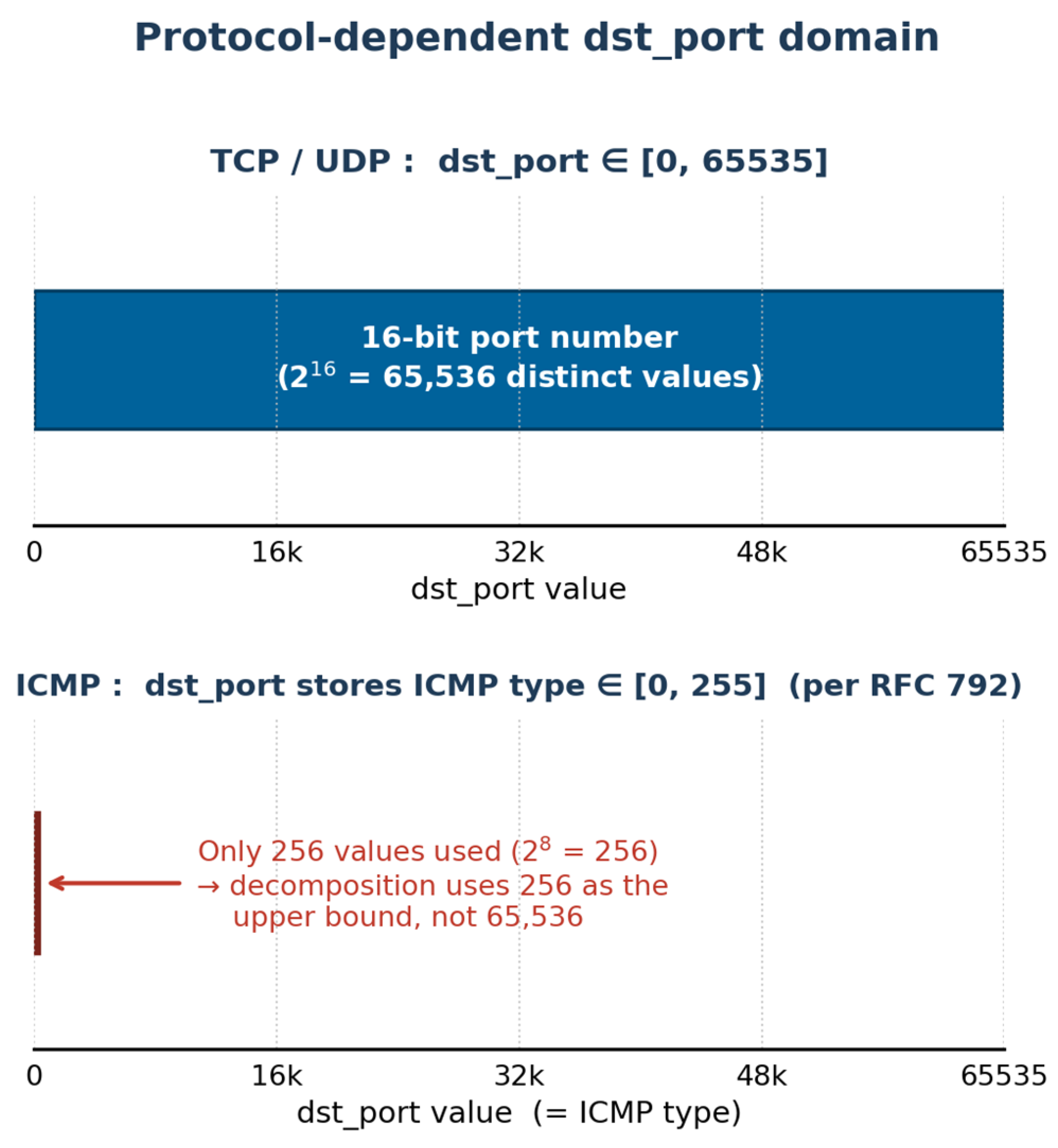
Figure 2.
The six-stage LRF-to-TRF conversion pipeline. Stage 2 (Deterministic Triad) is the sole anomaly detection component; the implementation is purely algorithmic with no machine-learning components.
Figure 2.
The six-stage LRF-to-TRF conversion pipeline. Stage 2 (Deterministic Triad) is the sole anomaly detection component; the implementation is purely algorithmic with no machine-learning components.
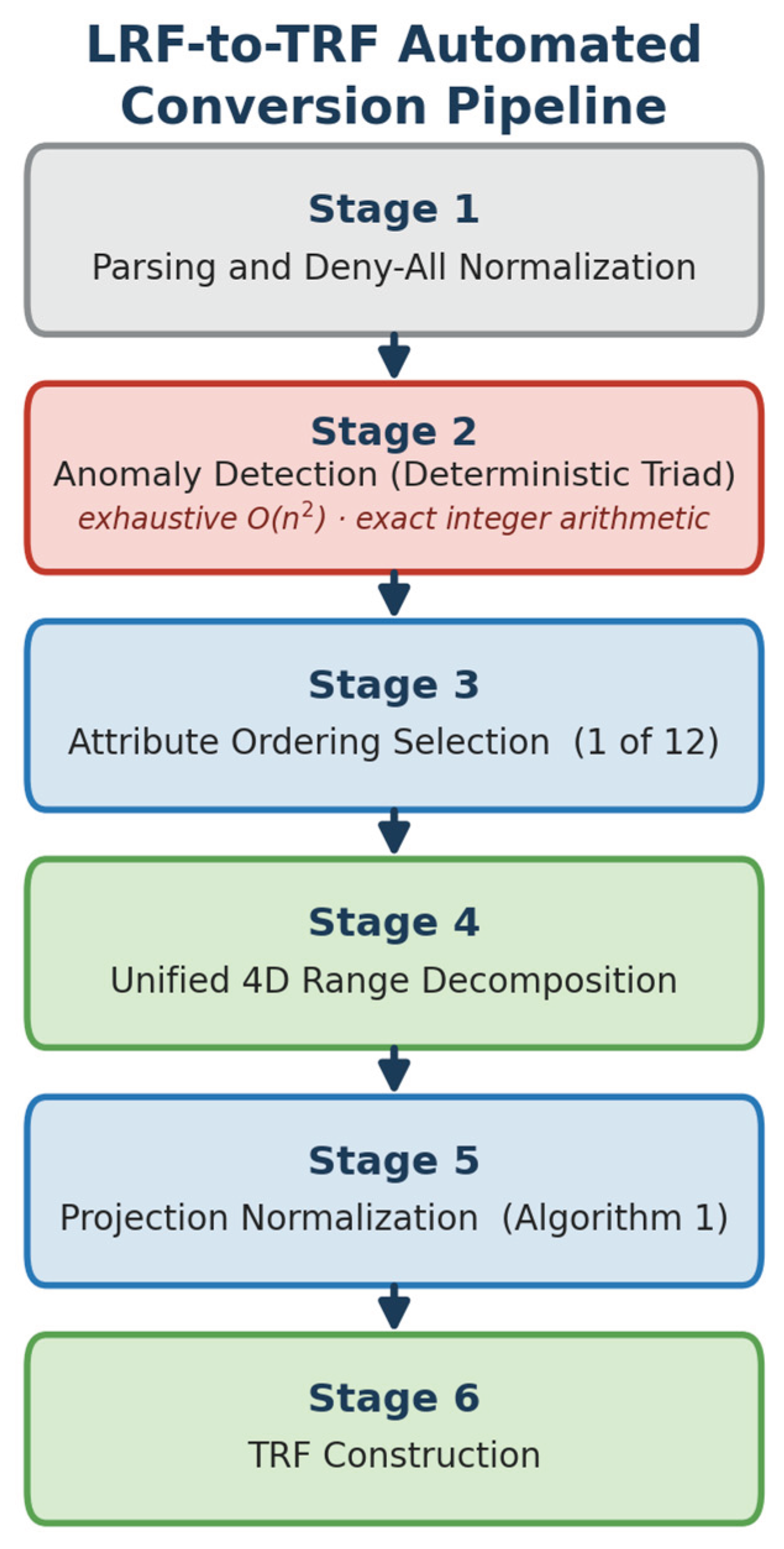
Figure 3.
The three LRF anomaly types in 2D match space. Shadow (top): full containment with conflicting actions. Redundancy (middle): full containment with identical actions. Correlation (bottom): partial overlap; neither rule contains the other.
Figure 3.
The three LRF anomaly types in 2D match space. Shadow (top): full containment with conflicting actions. Redundancy (middle): full containment with identical actions. Correlation (bottom): partial overlap; neither rule contains the other.
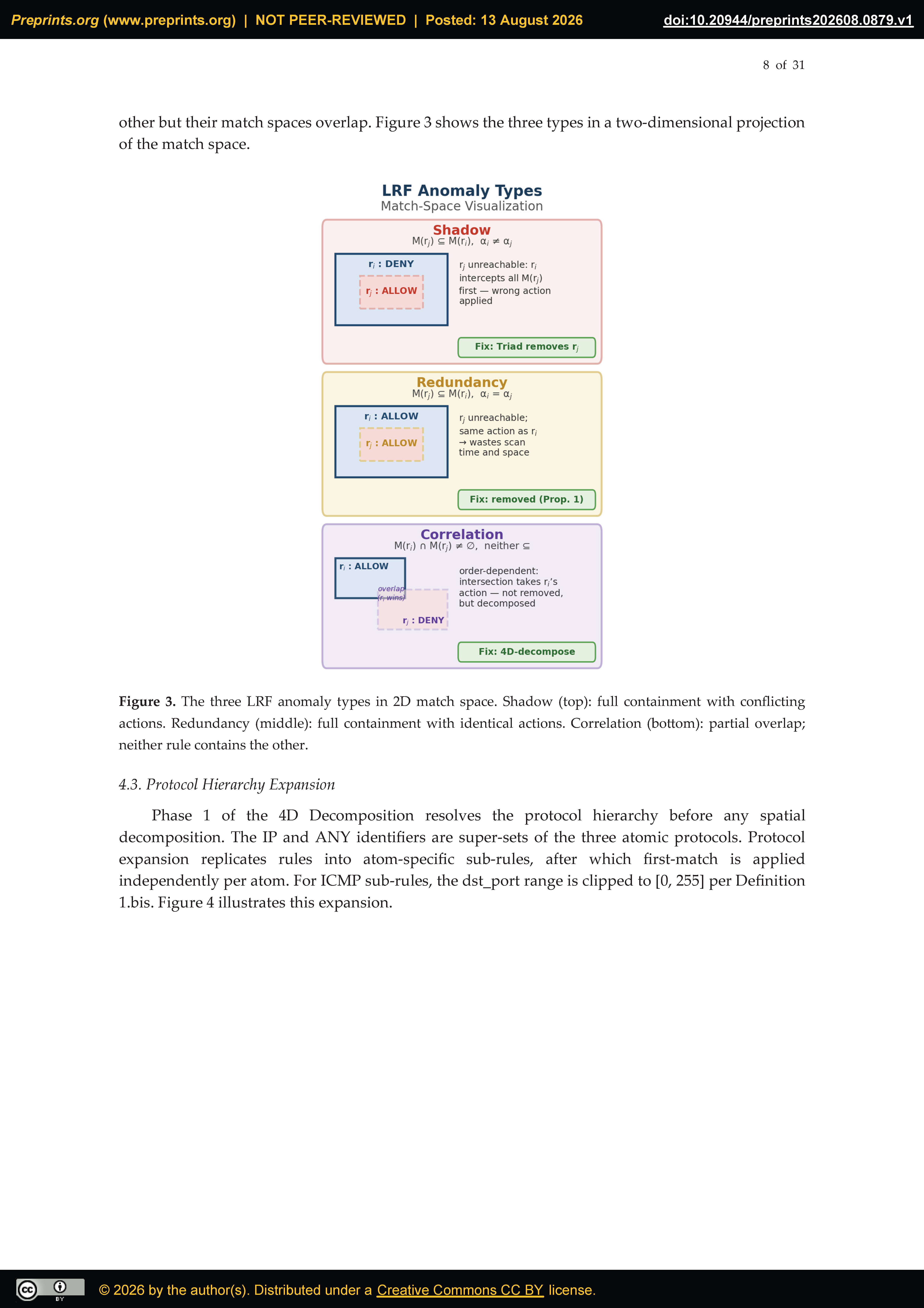
Figure 4.
Protocol hierarchy expansion (Phase 1 of Stage 4). After this phase, every rule carries a single atomic protocol identifier {TCP, UDP, ICMP}, and dst_port ranges of ICMP sub-rules are clipped to [0, 255].
Figure 4.
Protocol hierarchy expansion (Phase 1 of Stage 4). After this phase, every rule carries a single atomic protocol identifier {TCP, UDP, ICMP}, and dst_port ranges of ICMP sub-rules are clipped to [0, 255].
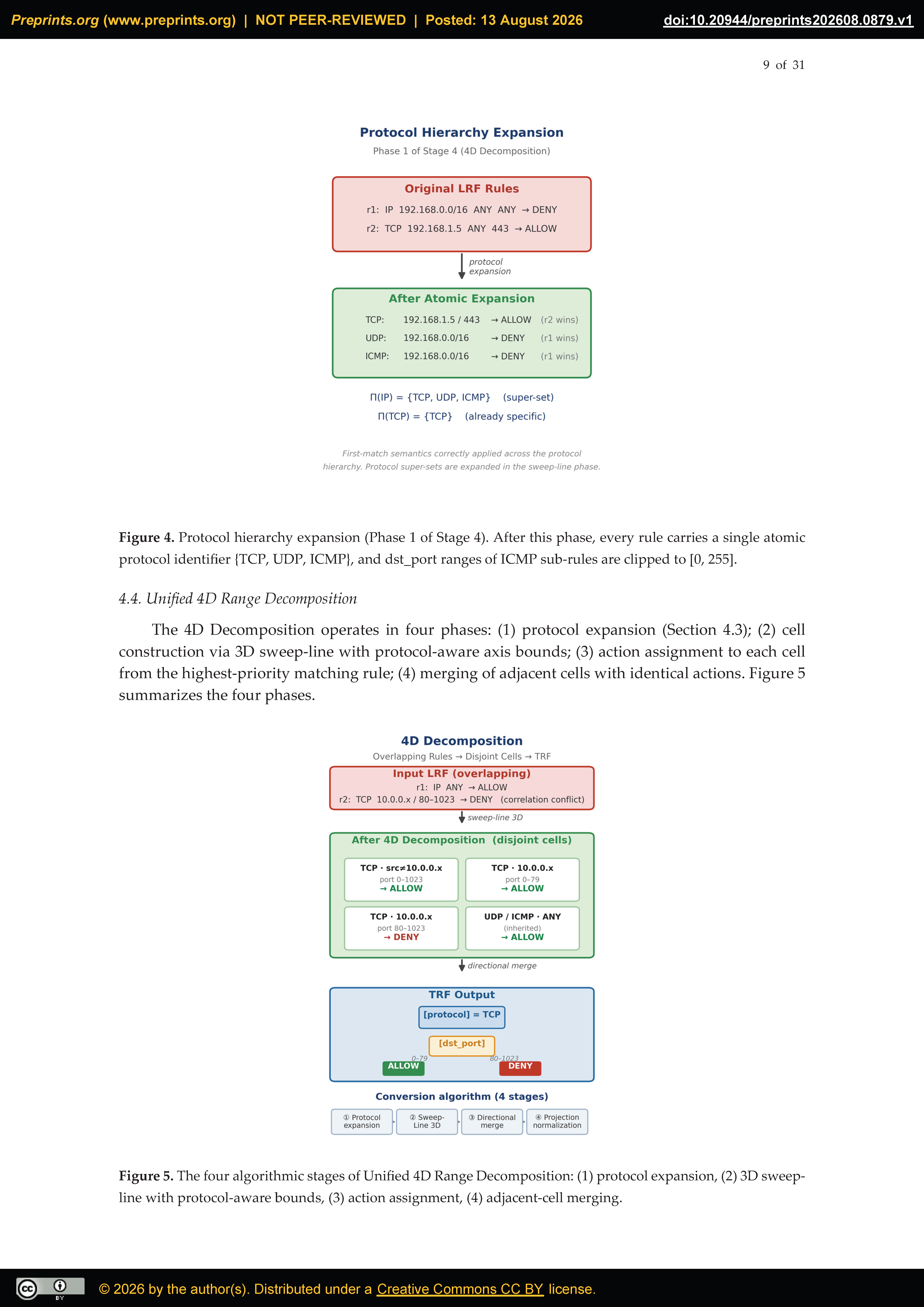
Figure 5.
The four algorithmic stages of Unified 4D Range Decomposition: (1) protocol expansion, (2) 3D sweep-line with protocol-aware bounds, (3) action assignment, (4) adjacent-cell merging.
Figure 5.
The four algorithmic stages of Unified 4D Range Decomposition: (1) protocol expansion, (2) 3D sweep-line with protocol-aware bounds, (3) action assignment, (4) adjacent-cell merging.
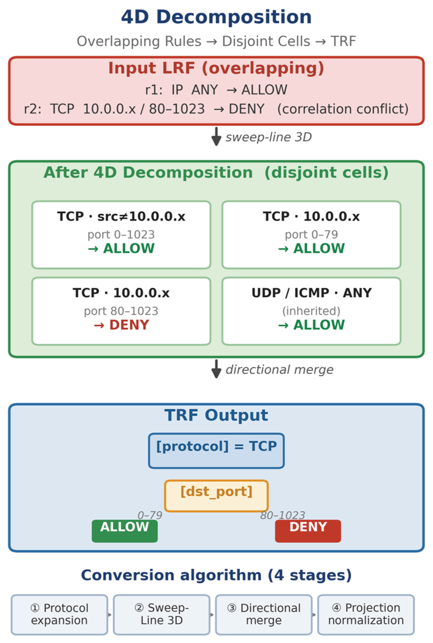
Figure 6.
Conversion time breakdown at n=400 (Ordering 4). Projection Normalization (Stage 5) dominates at approximately 55% of total conversion time, confirming its O(N²) complexity as the bottleneck.
Figure 6.
Conversion time breakdown at n=400 (Ordering 4). Projection Normalization (Stage 5) dominates at approximately 55% of total conversion time, confirming its O(N²) complexity as the bottleneck.
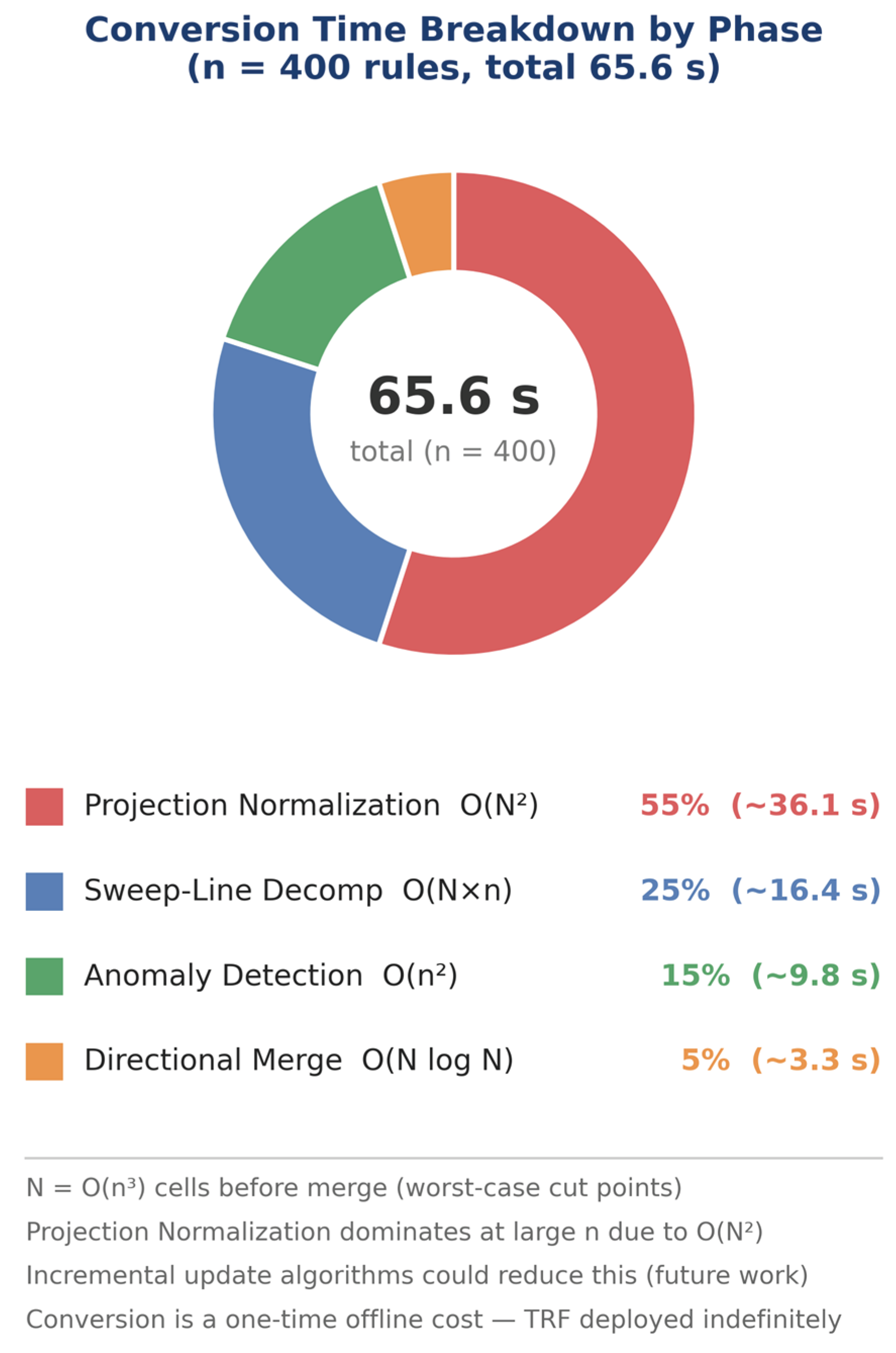
Figure 7.
Projection Normalization (Algorithm 1). Before normalization: two sibling nodes have overlapping dst_port ranges. After normalization: cut-points are unified and cells re-cut so that each packet matches exactly one node.
Figure 7.
Projection Normalization (Algorithm 1). Before normalization: two sibling nodes have overlapping dst_port ranges. After normalization: cut-points are unified and cells re-cut so that each packet matches exactly one node.
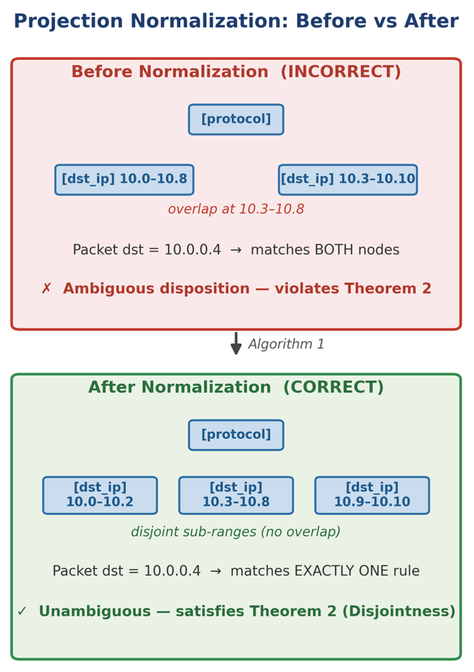
Figure 8.
End-to-end formal correctness chain. Proposition 2 establishes anomaly detection completeness; Proposition 1 proves semantic preservation through Stage 2; Theorems 1 and 2 establish TRF correctness and disjointness; Corollary 1 combines all results.
Figure 8.
End-to-end formal correctness chain. Proposition 2 establishes anomaly detection completeness; Proposition 1 proves semantic preservation through Stage 2; Theorems 1 and 2 establish TRF correctness and disjointness; Corollary 1 combines all results.
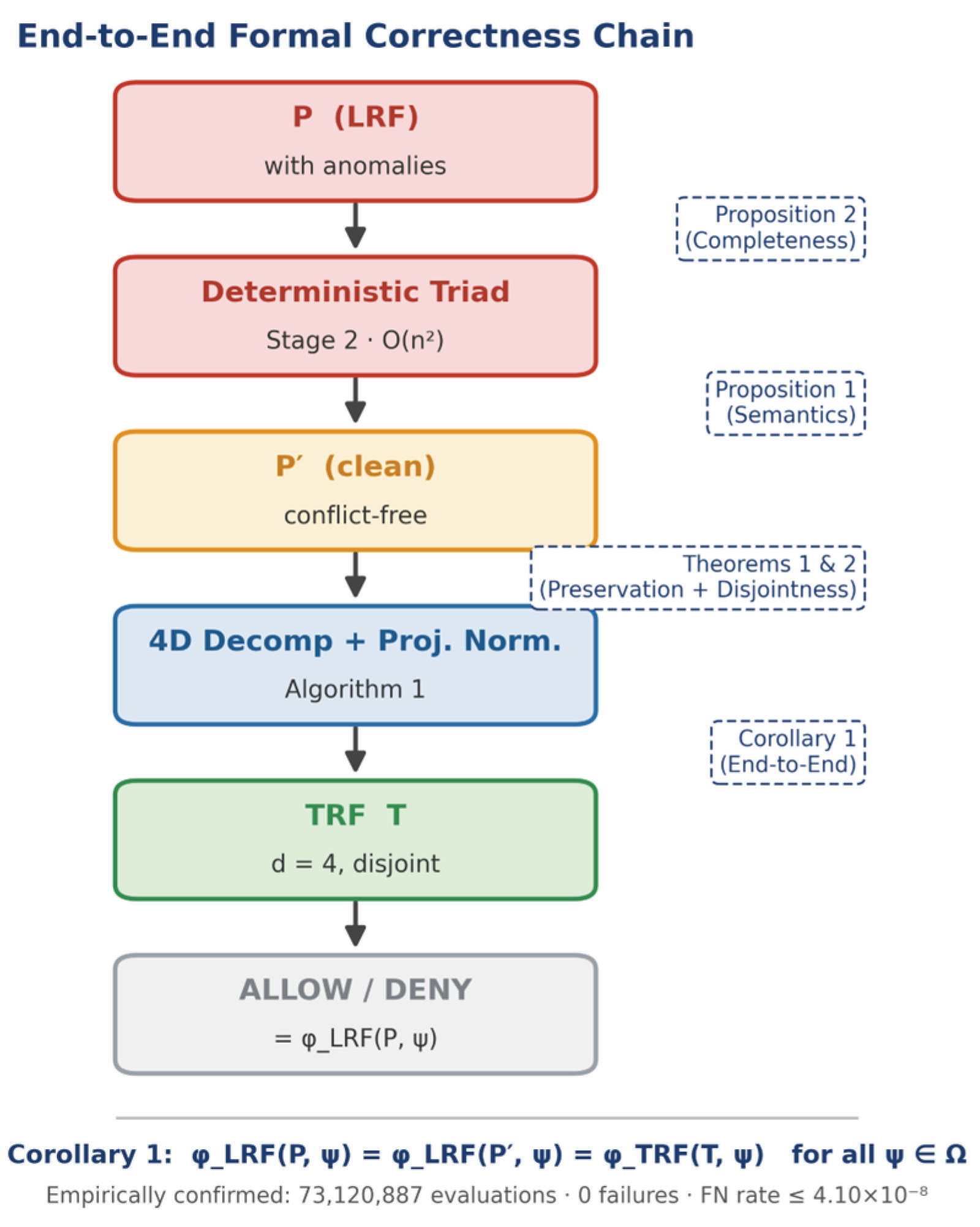
Figure 9.
TRF anatomy with attribute levels. Internal nodes carry attribute labels from ordering A*; edge ranges at every level are non-overlapping (Theorem 2). Each root-to-leaf path corresponds to exactly one cell from the 4D Decomposition.
Figure 9.
TRF anatomy with attribute levels. Internal nodes carry attribute labels from ordering A*; edge ranges at every level are non-overlapping (Theorem 2). Each root-to-leaf path corresponds to exactly one cell from the 4D Decomposition.
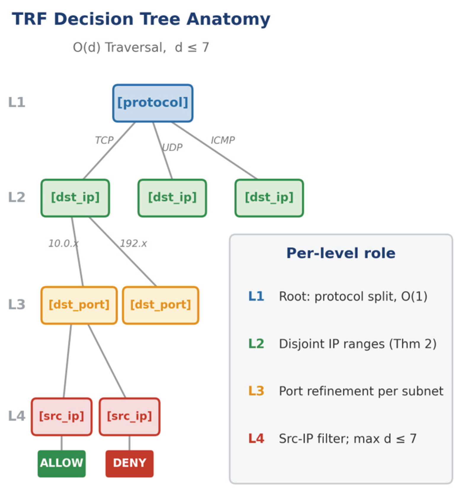
Figure 10.
Anomaly detection results across 7 anomaly types × 2 size categories (Small: 1–25 rules; Medium: 26–100 rules) × 500 trials (7,000 trials total). Total TP = 20,868; FP = FN = 0 in every trial. TP > trial count because multi-anomaly configurations inject 4–5 anomalies per trial.
Figure 10.
Anomaly detection results across 7 anomaly types × 2 size categories (Small: 1–25 rules; Medium: 26–100 rules) × 500 trials (7,000 trials total). Total TP = 20,868; FP = FN = 0 in every trial. TP > trial count because multi-anomaly configurations inject 4–5 anomalies per trial.
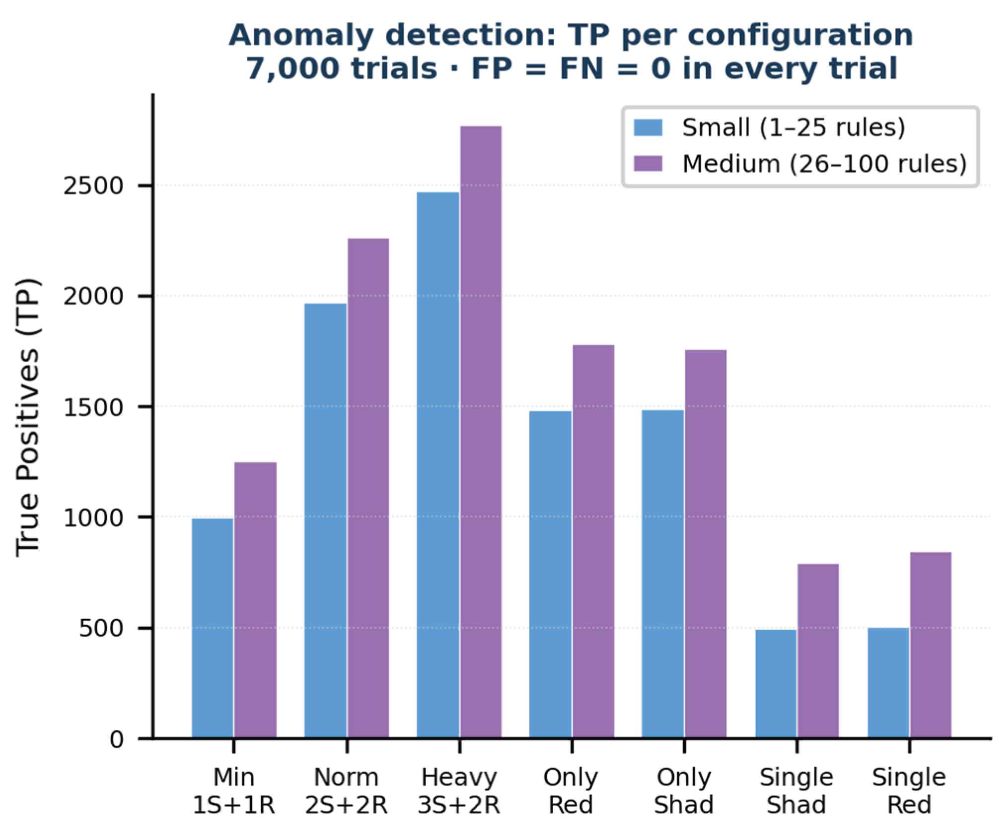
Figure 11.
(a) Match latency: TRF vs LRF across n ∈ {5,10,25,50,100,200,400} (scalability benchmark); size-category shading. Crossover at n≈100 (Medium). (b) Python-level TRF/LRF speedup per n; at n=400 (Large): 3.47×. Compiled Cython crossover at n≈4 (see Section 6.8).
Figure 11.
(a) Match latency: TRF vs LRF across n ∈ {5,10,25,50,100,200,400} (scalability benchmark); size-category shading. Crossover at n≈100 (Medium). (b) Python-level TRF/LRF speedup per n; at n=400 (Large): 3.47×. Compiled Cython crossover at n≈4 (see Section 6.8).
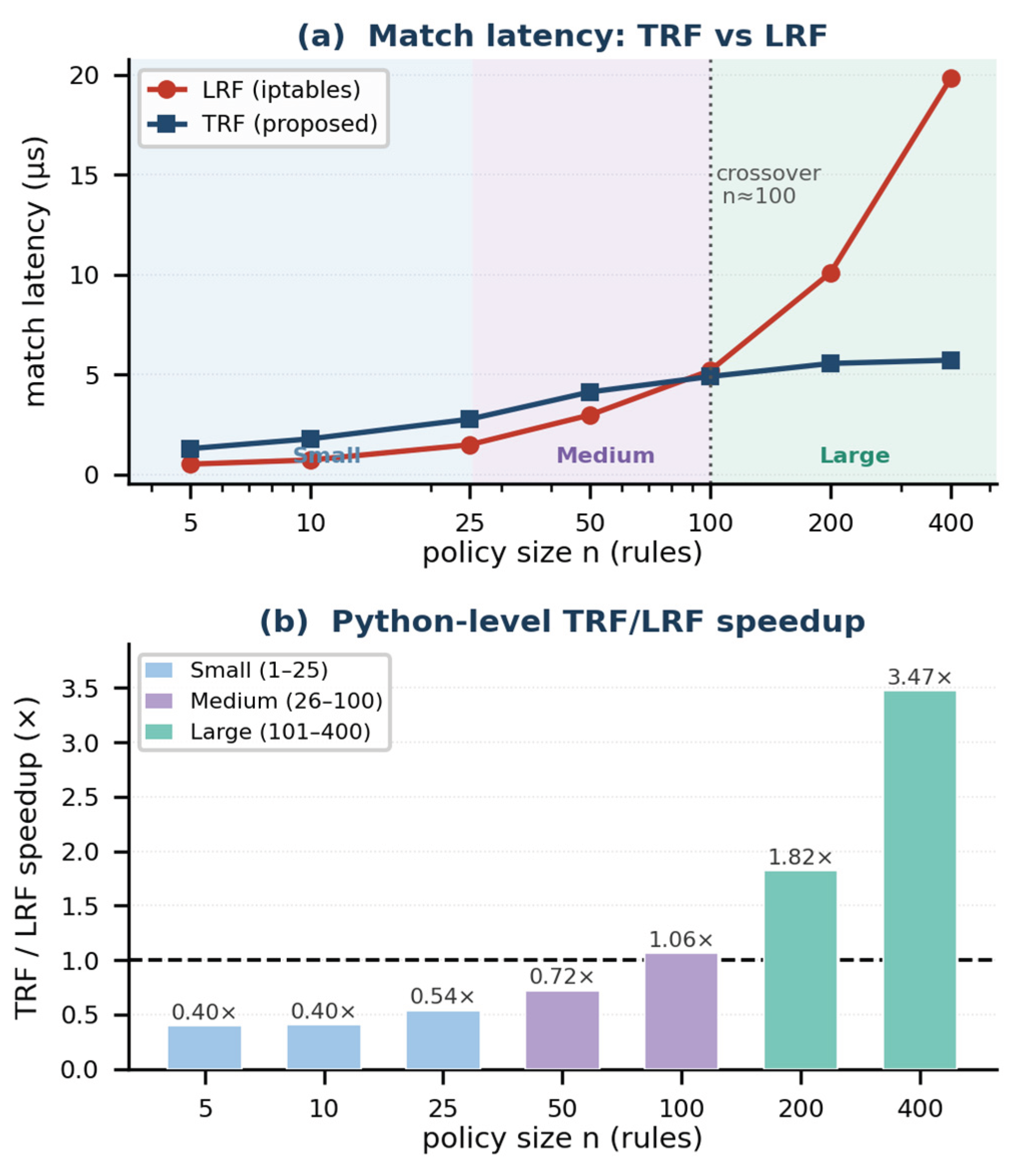
Figure 12.
Per-policy conversion time as a function of n. Super-linear growth is dominated by O(N²) Projection Normalization.
Figure 12.
Per-policy conversion time as a function of n. Super-linear growth is dominated by O(N²) Projection Normalization.
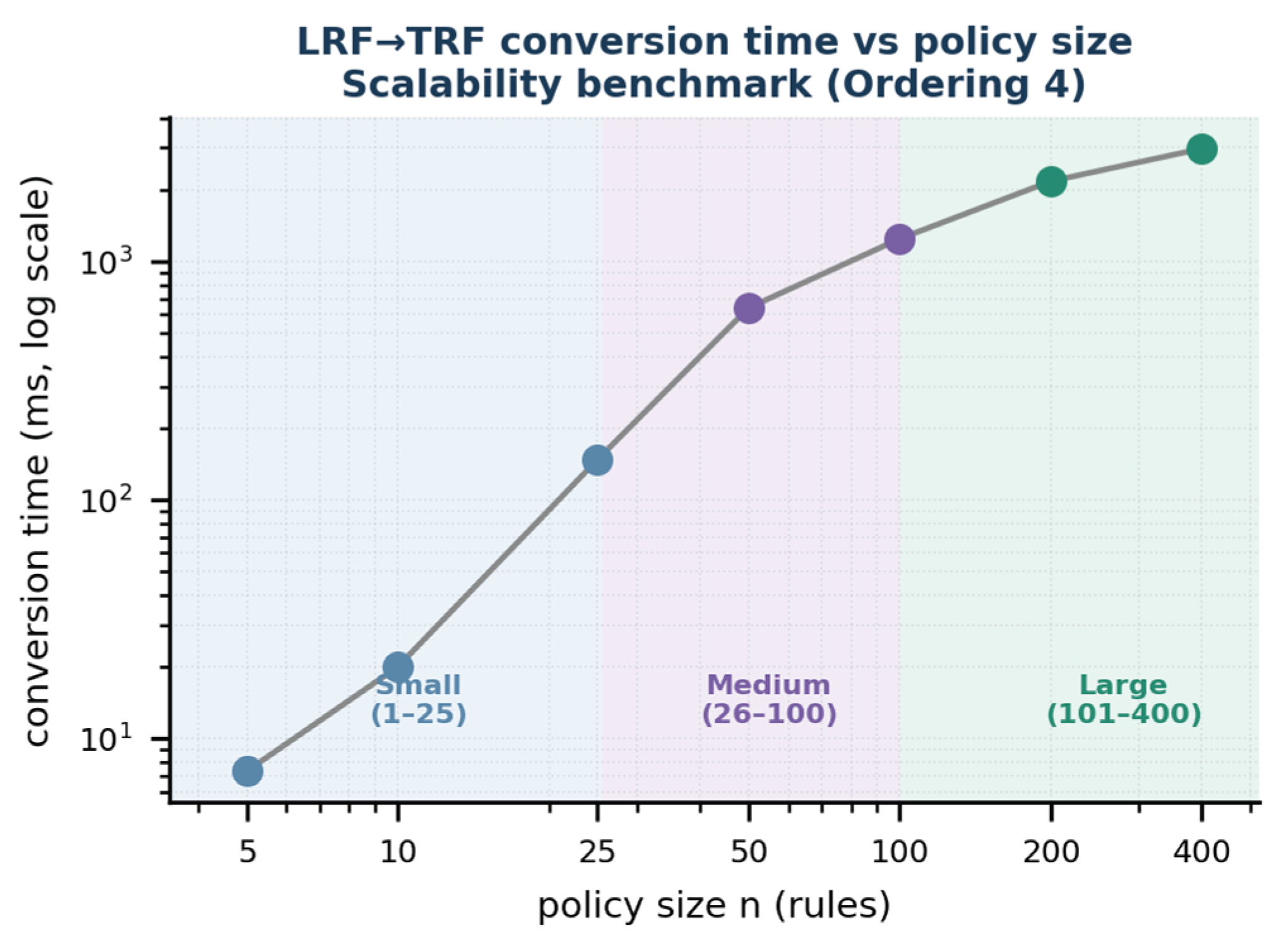
Figure 13.
Full experimental pipeline across six verification steps. All results feed into the main contributions: Table 2, Table 3, Table 4 and Table 5 and Figure 10, Figure 11, Figure 12, Figure 13, Figure 14 and Figure 15 collectively confirm semantic fidelity (Corollary 1), anomaly detection (Proposition 2), O(d) empirical matching (d = 4), and the scale-aware ordering finding.
Figure 13.
Full experimental pipeline across six verification steps. All results feed into the main contributions: Table 2, Table 3, Table 4 and Table 5 and Figure 10, Figure 11, Figure 12, Figure 13, Figure 14 and Figure 15 collectively confirm semantic fidelity (Corollary 1), anomaly detection (Proposition 2), O(d) empirical matching (d = 4), and the scale-aware ordering finding.
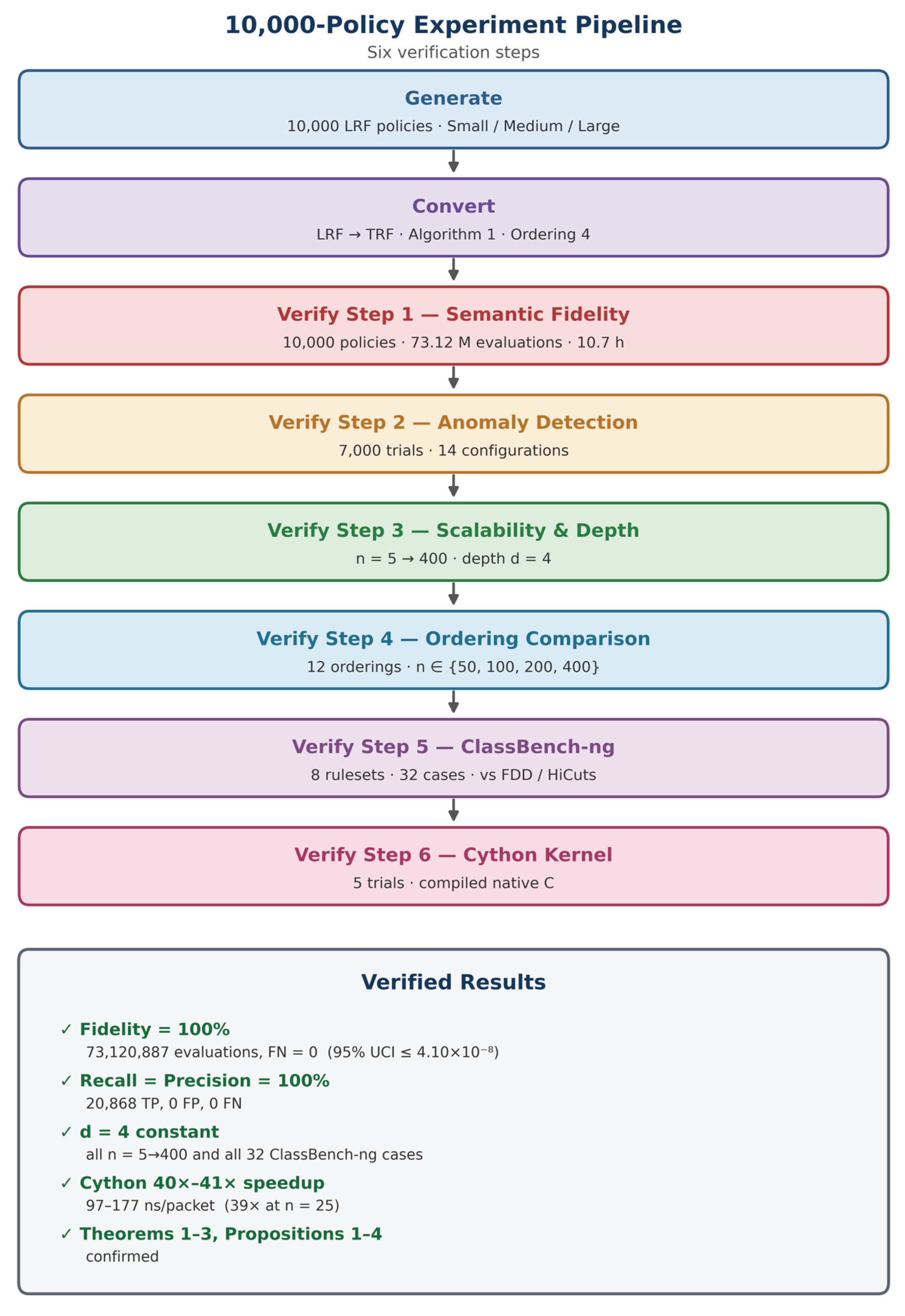
Figure 14.
Match latency (top) and per-ruleset speedup (bottom) on ClassBench-ng rulesets, averaged over 8 rulesets. HiCuts achieves lower per-packet latency due to leaf-level linear scan at binth=8, but TRF and FDD provide deterministic O(d) bounds.
Figure 14.
Match latency (top) and per-ruleset speedup (bottom) on ClassBench-ng rulesets, averaged over 8 rulesets. HiCuts achieves lower per-packet latency due to leaf-level linear scan at binth=8, but TRF and FDD provide deterministic O(d) bounds.
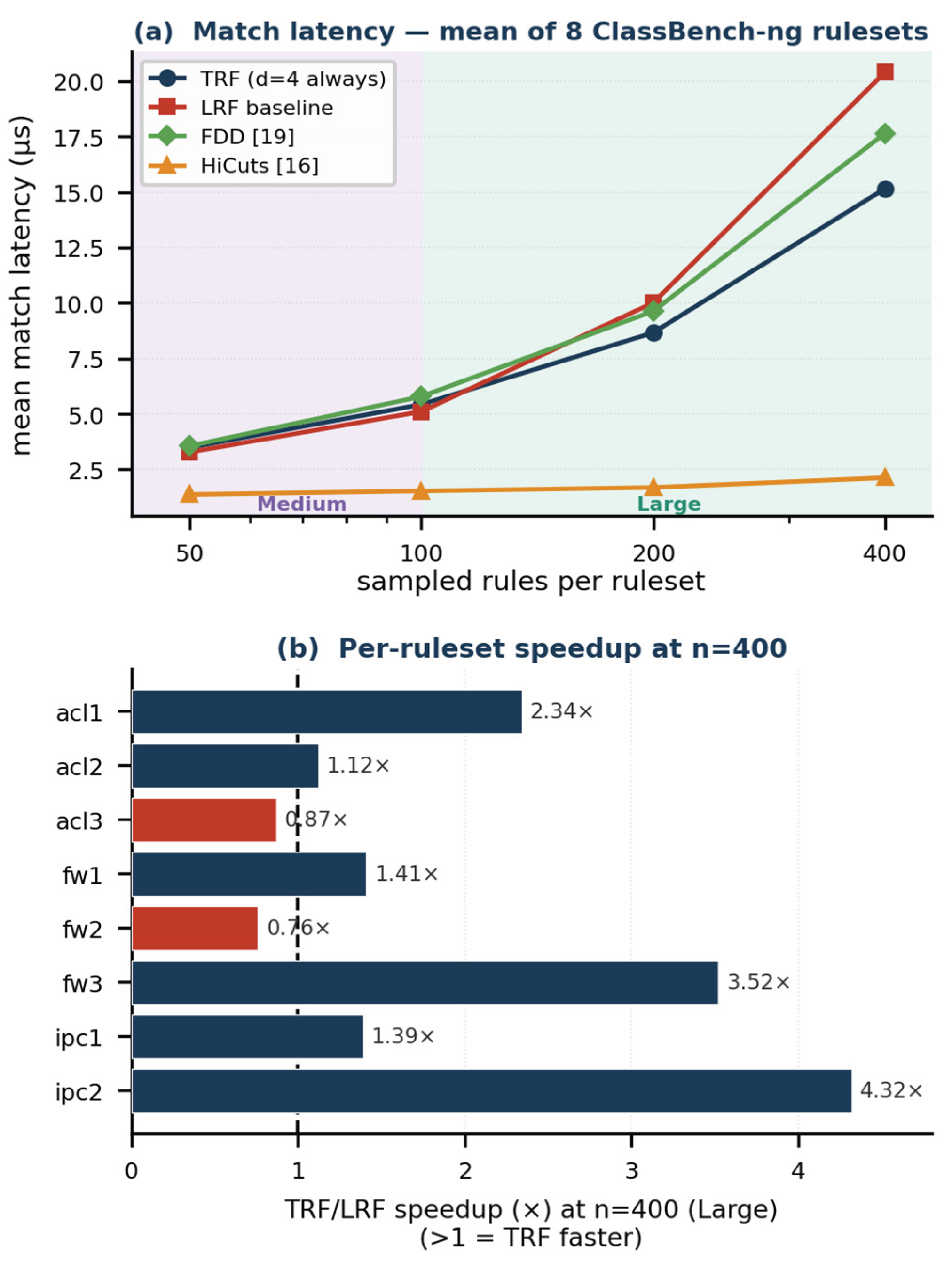
Figure 15.
Tree depth across 32 ClassBench-ng cases. TRF (and FDD) achieve d = 4 across all 32 cases, well within the theoretical d ≤ 7 bound. HiCuts depth varies from 1 to 12 across the 32 cases (2 to 12 at n=400), depending on ruleset complexity; six of the eight rulesets reach depth 12 at n=400, while FW2 never exceeds depth 2.
Figure 15.
Tree depth across 32 ClassBench-ng cases. TRF (and FDD) achieve d = 4 across all 32 cases, well within the theoretical d ≤ 7 bound. HiCuts depth varies from 1 to 12 across the 32 cases (2 to 12 at n=400), depending on ruleset complexity; six of the eight rulesets reach depth 12 at n=400, while FW2 never exceeds depth 2.
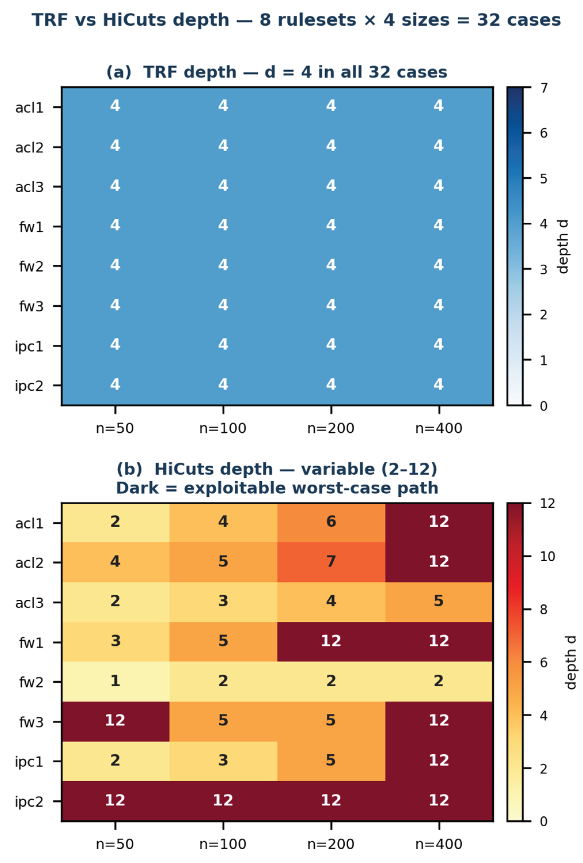

Table 1.
The twelve valid attribute orderings. Observed d = empirically observed depth. PF = protocol-first; PE = protocol-elsewhere.
Table 1.
The twelve valid attribute orderings. Observed d = empirically observed depth. PF = protocol-first; PE = protocol-elsewhere.
| ID | Ordering A* | Type | d obs. |
| 1 | protocol → src_ip → dst_ip → dst_port | PF | 4 |
| 2 | protocol → src_ip → dst_port → dst_ip | PF | 4 |
| 3 | protocol → dst_ip → src_ip → dst_port | PF | 4 |
| 4 | protocol → dst_ip → dst_port → src_ip [default] | PF | 4 |
| 5 | protocol → dst_port → src_ip → dst_ip | PF | 4 |
| 6 | protocol → dst_port → dst_ip → src_ip | PF | 4 |
| 7 | src_ip → protocol → dst_ip → dst_port | PE | 4 |
| 8 | src_ip → protocol → dst_port → dst_ip | PE | 4 |
| 9 | src_ip → dst_ip → protocol → dst_port | PE | 4 |
| 10 | dst_ip → protocol → src_ip → dst_port | PE | 4 |
| 11 | dst_ip → protocol → dst_port → src_ip | PE | 4 |
| 12 | dst_ip → src_ip → protocol → dst_port | PE | 4 |
Table 2.
Semantic fidelity results (10,000-policy dataset, Ordering 4).
| Category | Policies | Evaluations | FN | FN rate ≤ (95% UCI) |
| Small (1–25) | 3,333 | 15.59 M | 0 | 1.92×10⁻⁷ |
| Medium (26–100) | 3,334 | 23.47 M | 0 | 1.28×10⁻⁷ |
| Large (101–400) | 3,333 | 34.06 M | 0 | 8.81×10⁻⁸ |
| TOTAL | 10,000 | 73.12 M | 0 | 4.10×10⁻⁸ |
FN = False Negatives (TRF ≠ LRF). 95% upper-CI computed using the Rule of Three (3/N).
Table 3.
Ordering benchmark results at n ∈ {50,100,200,400} (10,000-policy dataset, 10 independent trials per condition). r_rb = matched-pairs rank-biserial correlation (effect size); Holm p = Holm-Bonferroni-adjusted p-value (all 5 metrics × 4 sizes = 20 comparisons corrected jointly). Protocol-first (PF) dominates structural metrics at all sizes; timing advantages reach confirmed statistical equivalence (TOST) at n=200 (not tested at n=400). ¹Peak memory measured via tracemalloc (Python’s built-in memory profiler), not sys.getsizeof. ²TOST equivalence was evaluated only at n=100 and n=200; n=400 was not tested for equivalence.
Table 3.
Ordering benchmark results at n ∈ {50,100,200,400} (10,000-policy dataset, 10 independent trials per condition). r_rb = matched-pairs rank-biserial correlation (effect size); Holm p = Holm-Bonferroni-adjusted p-value (all 5 metrics × 4 sizes = 20 comparisons corrected jointly). Protocol-first (PF) dominates structural metrics at all sizes; timing advantages reach confirmed statistical equivalence (TOST) at n=200 (not tested at n=400). ¹Peak memory measured via tracemalloc (Python’s built-in memory profiler), not sys.getsizeof. ²TOST equivalence was evaluated only at n=100 and n=200; n=400 was not tested for equivalence.
| Metric | n=50 | n=100 | n=200 | n=400 | r_rb | Holm p | Sig. |
| Tree mem. | 1.49× | 1.25× | 1.10× | 1.03× | 1.00 | 0.0195 | * (all n) |
| Nodes | 1.93× | 1.60× | 1.39× | 1.29× | 1.00 | 0.0195 | * (all n) |
| Match lat. | 1.15× | 1.06× | 0.99× | 0.95× | -0.67–1.00 | 0.0195–1 | *→ns |
| Conv. time | 1.34× | 1.12× | 0.97× | 0.93× | -1.00–1.00 | 0.0195–1 | *→ns |
| Peak mem.¹ | 1.56× | 1.29× | 1.11× | 1.02× | 0.89–1.00 | 0.0195–0.0244 | * (all n) |
Table 4.
ClassBench-ng comparison results (TRF vs FDD-style fixed-order ablation, HiCuts, and LRF), n=400 (Large), mean of 8 rulesets.
Table 4.
ClassBench-ng comparison results (TRF vs FDD-style fixed-order ablation, HiCuts, and LRF), n=400 (Large), mean of 8 rulesets.
| Engine | Build (ms) | Depth | Match (μs) | Notes |
| LRF | ~0 | n/a | 20.41 | Linear scan baseline (no tree) |
| TRF (proposed) | — | 4 | 15.16 | 12 orderings, ICMP-aware, d = 4 (all 32 cases) |
| FDD [19] | — | 4 | 17.65 | Single ordering only |
| HiCuts [16] | — | 2–12 | 2.12 | Variable depth 2–12, no worst-case bound |
Table 5.
Compiled Cython kernel performance. 5 trials, 5,000 packets per trial.
| n | Python (μs) | Cython (μs) | Speedup | TRF nodes / edges |
| 25 | 2.64 | 0.0674 | 39× | 23,937 / 23,936 |
| 50 | 3.88 | 0.0972 | 40× | 84,753 / 84,752 |
| 100 | 4.86 | 0.1198 | 40× | 191,080 / 191,079 |
| 200 | 6.63 | 0.1654 | 40× | 445,567 / 445,566 |
| 400 | 7.14 | 0.1772 | 41× | 596,784 / 596,783 |
Table 6.
Large-scale conversion results (50,000-policy dataset). All policies achieve TRF depth d = 4. Conversion time follows the same O(N²) trend as the original 10,000-policy dataset (Figure 12).
Table 6.
Large-scale conversion results (50,000-policy dataset). All policies achieve TRF depth d = 4. Conversion time follows the same O(N²) trend as the original 10,000-policy dataset (Figure 12).
| Category | Policies | TRF depth | Mean conv. time (s) | Std conv. time (s) | Max conv. time (s) | Mean nodes |
| Small (1–25) | 14,427 | 4 | 0.072 | 0.08 | 0.68 | 355 |
| Medium (26–100) | 18,133 | 4 | 1.428 | 1.181 | 7.35 | 3,064 |
| Large (101–400) | 17,440 | 4 | 10.445 | 6.219 | 36.10 | 11,377 |
| TOTAL | 50,000 | 4 | 4.18* | — | 36.10 | — |
*Overall mean across all 50,000 policies (total conversion time 209,092 s = 58.1 h).
Table 7.
Cross-platform scalability comparison. Main = Intel Core 5 210H (8C/12T, 32 GB, Windows 11). 2nd = Intel Core i7-8700 (6C/12T, 16 GB, Windows 11). TRF depth d = 4 on both platforms at every size.
Table 7.
Cross-platform scalability comparison. Main = Intel Core 5 210H (8C/12T, 32 GB, Windows 11). 2nd = Intel Core i7-8700 (6C/12T, 16 GB, Windows 11). TRF depth d = 4 on both platforms at every size.
| n | Depth | LRF μs (Main) | LRF μs (2nd) | TRF μs (Main) | TRF μs (2nd) | Speedup (Main) | Speedup (2nd) |
| 5 | 4 | 0.51 | 0.61 | 1.29 | 1.52 | 0.40× | 0.40× |
| 10 | 4 | 0.72 | 0.90 | 1.78 | 1.96 | 0.40× | 0.46× |
| 25 | 4 | 1.48 | 1.80 | 2.76 | 3.21 | 0.54× | 0.56× |
| 50 | 4 | 2.97 | 3.45 | 4.12 | 4.79 | 0.72× | 0.72× |
| 100 | 4 | 5.20 | 6.47 | 4.90 | 5.88 | 1.06× | 1.10× |
| 200 | 4 | 10.09 | 12.55 | 5.55 | 6.77 | 1.82× | 1.85× |
| 400 | 4 | 19.84 | 23.84 | 5.71 | 7.03 | 3.47× | 3.39× |
Disclaimer/Publisher’s Note: The statements, opinions and data contained in all publications are solely those of the individual author(s) and contributor(s) and not of MDPI and/or the editor(s). MDPI and/or the editor(s) disclaim responsibility for any injury to people or property resulting from any ideas, methods, instructions or products referred to in the content. |
© 2026 by the authors. Licensee MDPI, Basel, Switzerland. This article is an open access article distributed under the terms and conditions of the Creative Commons Attribution (CC BY) license (http://creativecommons.org/licenses/by/4.0/).
Copyright: This open access article is published under a Creative Commons CC BY 4.0 license, which permit the free download, distribution, and reuse, provided that the author and preprint are cited in any reuse.