
Submitted:
12 August 2026
Posted:
13 August 2026
You are already at the latest version
Abstract
Hospital pharmacy replenishment decisions are made under demand uncertainty, where stockouts may compromise service continuity and overstock may immobilize scarce resources. This study proposes a demand-profile-informed framework for selecting probabilistic inventory models for medication supply decisions. Monthly demand records and consolidated operational cost parameters for 13 medicines over 48 months were analyzed to characterize high-, medium-, low-, and intermittent-demand profiles. Candidate models included normal, gamma, negative binomial type II, and zero-inflated negative binomial distributions. Each fitted distribution was embedded in a two-stage stochastic inventory-cost model, where distribution-specific scenarios determined first-stage replenishment quantities and binary ordering decisions, and second-stage shortage and overstock outcomes were evaluated. A Monte Carlo simulation study assessed model behavior under controlled levels of demand, variability, zero-demand frequency, trend, and shortage-cost exposure. Empirical results showed substantial demand heterogeneity across medicines. Normal and gamma models provided the best statistical fit for most recurrent-demand medicines, whereas zero-inflated negative binomial models dominated several intermittent-demand cases. Model-based replenishment reduced realized costs for 11 of the 13 medicines, with percentage savings ranging from 15.4% to 99.3% among improved cases; however, one medicine showed a negative saving, confirming that statistical fit and operational cost performance may diverge. Simulation results identified zero-demand frequency as the main driver of model selection, with zero-inflated models becoming dominant once zero-demand months were introduced. The proposed framework provides interpretable decision rules to support differentiated, data-driven replenishment decisions in hospital pharmacy management.
Keywords:
hospital pharmacy
; medication supply
; inventory management
; two-stage stochastic programming
; probabilistic demand modelling
; sample-average approximation
; intermittent demand
; zero-inflated negative binomial
; inventory-cost evaluation
; decision support
1. Introduction
Medication supply in hospital pharmacies is a high-stakes operational process because replenishment decisions must be made before future demand, stockout risk, and procurement conditions are fully observed [1]. Shortages may compromise patient-care activities, increase the workload required to manage supply disruptions, and force emergency procurement or therapeutic substitution, whereas excessive inventory immobilizes scarce resources and increases storage, expiration, and obsolescence risks [2]. For this reason, hospital medication inventory should be framed as a decision-making problem under uncertainty, where replenishment policies must balance purchasing costs, holding costs, safety-stock requirements, shortage risk, and service-level requirements in settings characterized by variable demand and constrained resources [3,4,5,6].
Hospital pharmacy managers have traditionally used practical classification and replenishment tools to organize inventory decisions. These include ABC analysis, where items are grouped into A, B, and C classes according to their contribution to annual consumption value or expenditure, and Vital, Essential, and Non-essential/Desirable (VEN/VED) matrices, where medicines are classified according to clinical criticality [7,8]. These tools are useful for prioritization, but they do not by themselves determine which probabilistic demand model should be used when medicines differ in demand volume, variability, zero-demand frequency, shortage exposure, and cost structure [9,10].
Although previous studies have advanced medication inventory optimization under shortage risk [4,5,6], multicriteria and classification-based inventory management [9,11], simulation-based inventory policies [10], digital decision support and medication-management technologies [12,13], and stochastic inventory modelling under uncertain demand [14,15], there is still limited evidence on how to select probabilistic inventory models according to observable medication demand profiles. This creates a specific gap for hospital pharmacy inventory research. More specifically, previous studies rarely integrate: (i) empirical hospital pharmacy data, (ii) classification of medication demand into operationally meaningful profiles, (iii) comparison of alternative probability distributions, (iv) two-stage stochastic inventory-cost evaluation, where distribution-specific demand scenarios determine first-stage replenishment decisions and second-stage shortage and overstock outcomes, and (v) simulation-based decision rules that can be interpreted by hospital pharmacy decision makers [9,10,14,16,17].
The present study addresses this gap by proposing a demand-profile-informed decision-support framework for hospital pharmacy medication supply under uncertainty. The empirical component uses real monthly medication demand and cost data from a public hospital pharmacy to classify products, fit alternative probabilistic demand models, generate distribution-specific demand scenarios, and evaluate inventory performance through a two-stage stochastic inventory-cost model. The simulation component generalizes the empirical setting by generating controlled demand scenarios that vary in demand level, variability, zero-demand frequency, temporal dependence, and shortage-cost exposure. This combined design allows the real hospital case to serve as both a calibration source and an illustrative application, while the simulation study supports more generalizable decision rules [10,14,16].
The core research question is therefore: How do medication demand profiles influence the performance of probabilistic inventory models for hospital pharmacy supply decisions, and under which simulated conditions does each modelling strategy perform best? This question is operationally relevant because a single inventory rule may perform differently for high-volume medicines, medium-demand products, low-demand medicines, and intermittent items, especially when shortage costs, replenishment constraints, and budgetary pressure are incorporated into the decision problem [4,5,9].
We test four working hypotheses. First, high- and medium-demand medicines with relatively stable consumption can be adequately represented by lower-complexity distributions such as the normal model, particularly when zero-demand months are absent or rare [14]. Second, low-demand and positively skewed medicines require non-negative asymmetric or count-based alternatives because symmetric approximations may underrepresent skewness and lower-bound constraints [14,18]. Third, intermittent demand with repeated zero months favors zero-inflated or occurrence–size modelling strategies, since zero-demand periods are a defining feature of intermittent and lumpy demand [16,19]. Fourth, inventory-cost performance may diverge from statistical fit, implying that the Akaike Information Criterion (AIC) or forecast error should not be used as the sole criterion for operational decision-making when holding costs, shortage costs, and service-level consequences are relevant [10,14,16].
The contribution of this article is threefold. First, it provides empirical evidence on how alternative probabilistic demand models behave across medication demand profiles in a hospital pharmacy. Second, it complements the empirical case with a simulation study designed to assess the robustness of model performance under controlled levels of demand variability, intermittency, and shortage-cost exposure. Third, it translates empirical and simulation results into interpretable decision rules that can support hospital pharmacy managers when selecting inventory models under uncertainty [9,10,13].
The remainder of the article is structured as follows. Section 2 summarizes the state of the art and positions the contribution. Section 3 describes the empirical case, operational parameters, demand-profile classification, probabilistic models, stochastic inventory evaluation, simulation design, reproducibility workflow, and decision-rule extraction. Section 4 presents empirical and simulation results. Section 5 discusses the findings, implications for decision makers, limitations, and future research. Section 6 concludes.
2. State of the Art
This section reviews five research streams that are directly related to the proposed framework: classification-based inventory management, simulation and inventory-policy optimization, probabilistic and stochastic inventory modelling, intermittent-demand forecasting, and digital decision support in pharmacy practice. The purpose is not to restate the general importance of medication supply, which was introduced above, but to position the specific gap addressed by this study: the lack of an integrated framework that links medication demand profiles with probabilistic model selection, stochastic inventory-cost performance, simulation evidence, and interpretable decision rules.
A first stream focuses on classification-based inventory management. ABC analysis and VEN/VED matrices have been widely used in hospital pharmacy settings because they help managers prioritize items according to expenditure, demand relevance, and clinical importance [7,8,20]. However, hospital inventories are multidimensional: an item with low annual expenditure may still be operationally critical, difficult to substitute, or exposed to shortage risk. This explains why recent studies have argued for integrating expenditure-based and criticality-based classifications with broader decision-support criteria [11,21]. Multi-criteria decision-support models have therefore been proposed to classify medicines and materials more effectively than single-criterion approaches [9]. These studies are valuable for prioritization, but they generally do not determine which probabilistic demand model should be used for each medication profile, nor do they evaluate how distributional assumptions affect inventory-cost performance.
A second stream focuses on simulation and inventory-policy optimization. Simulation optimization has been applied to outpatient pharmacy inventory settings to determine minimum and maximum stock levels under cost and operational constraints, showing that optimized policies can reduce inventory costs compared with current settings [10]. Other optimization studies have addressed hospital drug shortages and supply-chain disruptions, emphasizing that stochastic demand, supplier unreliability, and service-level targets should be incorporated into replenishment decisions [4,5]. Pharmaceutical supply-chain reliability models have also emphasized that shortage risk depends on disruption frequency, recovery speed, and redundancy in supply configurations [6]. Nevertheless, these studies usually optimize a selected policy or supply-chain configuration, rather than deriving interpretable rules that guide the selection of probabilistic inventory models according to medication demand profiles.
A third stream addresses probabilistic and stochastic inventory modelling. In hospital pharmacy applications, lot-size models under uncertain demand have been formulated using stochastic programming and distributional features such as skewness and kurtosis [14]. This line of work is particularly relevant because medication demand may depart from normality: some products exhibit high and stable consumption, whereas others are skewed, overdispersed, low-volume, or intermittent. In this context, distributional assumptions are not only descriptive choices: they define the demand scenarios used by the stochastic program and can therefore affect first-stage order quantities, second-stage shortage or overstock outcomes, and realized inventory costs. However, the literature still tends to evaluate modelling strategies at the product or case-study level, without systematically translating demand characteristics into operational model-selection rules.
A fourth stream comes from intermittent-demand forecasting. Intermittent and lumpy demand are recognized as difficult to forecast because the time series include many zero-demand periods and irregular positive demand sizes. Critical reviews and recent methodological studies have shown that intermittent-demand problems often require methods that distinguish demand occurrence from demand size, and that forecast accuracy alone may not capture inventory consequences [16,17,18,19]. Although this literature is highly relevant for low-volume and sporadic medicines, most studies are developed in general supply-chain or spare-parts contexts rather than hospital pharmacy settings, and they are rarely integrated with stochastic inventory-cost evaluation.
A fifth stream focuses on digitalization and decision-support systems in pharmacy practice. Clinical decision-support systems have been used by clinical pharmacy teams to detect drug-related problems, while automation and digitalization studies have evaluated the economic implications of hospital medication-management technologies [12,13]. These contributions support the broader movement toward data-driven pharmacy management, but their primary focus is clinical decision support or technological return on investment, rather than probabilistic inventory-model selection for medication supply decisions.
Table 1 summarizes how these streams position the proposed framework. The common limitation is not the absence of inventory, forecasting, or decision-support research, but the lack of an integrated and interpretable framework that links medication demand profiles with probabilistic model selection, stochastic inventory-cost performance, simulation evidence, and practical decision rules for hospital pharmacy managers.
Based on this review, the proposed framework advances the literature in three ways. First, it treats medication demand heterogeneity as a central modelling issue rather than as a secondary descriptive feature. Second, it evaluates probabilistic models not only by statistical fit, but also by inventory-cost performance, shortage exposure, and savings relative to observed or baseline decisions. Third, it uses simulation to move beyond a single empirical case and derive decision rules that can be interpreted and potentially implemented by hospital pharmacy decision makers.
3. Materials and Methods
3.1. Study Design
This study was designed as a two-layer decision-support analysis for hospital pharmacy medication supply under demand uncertainty. The first layer was an empirical case study based on real medication demand and cost records from a public hospital pharmacy. This layer was used to characterize observed demand profiles, estimate probabilistic demand models, and evaluate one-cycle replenishment decisions under actual operational cost parameters. The second layer was a Monte Carlo simulation study designed to assess whether the empirical findings remained consistent under controlled combinations of demand level, variability, intermittency, temporal trend, and shortage-cost exposure.
The methodological rationale was that empirical data provide operational realism, whereas simulation allows systematic variation of conditions that cannot be fully observed in a single hospital case. This combined design is consistent with previous healthcare inventory studies that use simulation optimization to evaluate pharmacy replenishment policies, while extending them by explicitly linking probabilistic model choice to medication demand profiles and inventory-cost performance [10,14]. The stochastic inventory-evaluation component follows the logic of sample-average approximation and two-stage stochastic programming, where distribution-specific demand scenarios determine first-stage replenishment decisions and second-stage shortage and overstock outcomes before the selected decisions are assessed against realized demand [15].
3.2. Empirical Case Study
The empirical component used monthly demand records for 13 medicines dispensed by a hospital pharmacy over a 48-month period. The selected medicines represented four operational demand profiles: high-demand, medium-demand, low-demand, and intermittent-demand items. This selection was intended to reflect the type of heterogeneity commonly faced by hospital pharmacy managers, where medicines differ not only in average consumption, but also in variability, zero-demand frequency, acquisition cost, replenishment scale, and potential shortage consequences.
For each medicine, the empirical dataset included monthly demand, unit acquisition cost, initial inventory for the evaluation period, observed replenishment quantity, fixed ordering cost, unit holding cost, shortage-cost factor, and an operational replenishment-capacity parameter. The monthly demand series were used to fit candidate probability distributions and characterize demand profiles. The cost and inventory variables were used to evaluate the consequences of translating probabilistic demand models into replenishment decisions.
The replenishment-capacity parameter was defined as the maximum feasible replenishment level observed for each medicine during the calibration period. When the inventory model was expressed in monetary terms, this parameter was converted using the corresponding unit acquisition cost. This operational definition was adopted to represent a realistic one-cycle upper bound for replenishment decisions, consistent with the historical scale of procurement observed for each medicine.
The empirical evaluation used the first 47 monthly observations as the calibration window and the final month as the out-of-sample evaluation period. This structure allowed the probabilistic models to be fitted using historical information available before the decision period and then evaluated against subsequently observed demand. Thus, the empirical component reproduced the operational sequence faced by pharmacy decision makers: historical demand is observed, a replenishment decision is made under uncertainty, and the decision is later evaluated once actual demand is realized.
3.3. Data Consolidation and Operational Inputs
The expanded institutional datasets were used to consolidate the empirical inputs required for the decision-support framework. This consolidation did not change the structure of the simulation study, but it strengthened the empirical layer by clarifying which variables were used to construct demand profiles, fit probability distributions, define the observed replenishment decision, and evaluate inventory costs. Table 2 summarizes the main empirical inputs and their role in the analysis.
This consolidation is relevant because the empirical results depend not only on the demand series but also on how inventory decisions are economically evaluated. Consequently, the distributional-fit results should be interpreted as statistical evidence about historical demand, whereas the inventory-cost results should be interpreted as decision outcomes conditional on the consolidated operational parameters, initial stock, observed replenishment, replenishment bounds, and realized final-period demand.
3.4. Operational Cost Parameters
The empirical inventory-cost evaluation used medicine-level and institutional cost parameters. The unit acquisition cost represented the purchase price of medicine i. The initial inventory represented the available stock before the evaluation period. The observed replenishment quantity represented the real order quantity registered for the final evaluation period. The fixed ordering cost represented the administrative and operational cost of issuing an order, while the holding cost represented the cost of storing one unit during the decision period.
Shortage cost was represented as a proportional factor applied to the unit acquisition cost. Thus, the unit shortage cost was expressed as , where is the proportional shortage-cost factor. This formulation allows shortage-cost exposure to be incorporated into both the empirical evaluation and the simulation study. Because institutional definitions of shortage cost may differ depending on whether the objective is to represent only the additional emergency-procurement premium or the full replacement-cost burden, shortage-cost exposure was also considered in the simulation as a sensitivity dimension. This avoids making the results depend exclusively on a single accounting interpretation of stockout cost.
3.5. Demand-Profile Classification
Demand profiles were characterized using descriptive and structural indicators calculated from the calibration window. For each medicine i, the following indicators were computed: mean monthly demand , standard deviation , coefficient of variation , minimum demand, maximum demand, zero-demand share , and empirical skewness when applicable. These indicators were selected because segmentation according to consumption patterns, demand variability, and intermittency can support the selection of differentiated forecasting and inventory-control policies [22,23].
Medicines were assigned to operational demand profiles by combining their ABC demand suffixes with the empirical indicators. Within this study, high- and medium-demand profiles were operationally associated with positive demand during most or all months of the calibration window, whereas low-demand profiles were characterized by lower average consumption and greater relative variability. Intermittent-demand medicines were identified by repeated zero-demand periods separated by irregular positive-demand occurrences, consistent with established descriptions of intermittent demand patterns [23]. This combined classification reflects the broader inventory-management principle that hospital medicines should not be treated as homogeneous items, because expenditure, demand volume, clinical criticality, variability, and shortage exposure may require different managerial responses [9,22].
The classification was not used only as a descriptive label. It served as the main explanatory layer for comparing probabilistic demand models and deriving practical decision rules. In this sense, the methodological focus was not merely to determine which distribution fitted each medicine, but to evaluate whether observable demand-profile indicators could guide the selection of inventory models in a way that is interpretable for hospital pharmacy decision makers.
3.6. Justification of Candidate Probability Distributions
Four candidate probability distributions were evaluated: normal (NO), gamma (GA), negative binomial type II (NBII), and zero-inflated negative binomial (ZINBI). These distributions were selected to represent distinct assumptions regarding the support, symmetry, dispersion, and occurrence of zero observations in medication-demand data. Collectively, they cover approximately symmetric high-volume demand, positive right-skewed demand, overdispersed count demand, and overdispersed demand with excess zeros [24,25,26,27].
The normal distribution was included as a low-complexity benchmark for medicines with relatively high and stable demand. Normal approximations are commonly used in inventory-control settings because they provide a parsimonious and operationally interpretable representation when demand is sufficiently aggregated and its variability is moderate relative to the mean [24]. In this study, the normal distribution was therefore considered most plausible when demand was positive in most or all calibration periods and showed limited asymmetry. Nevertheless, because the distribution is symmetric and defined over the entire real line, it can assign positive probability to negative values and may provide a poor representation of low-volume, strongly right-skewed, or zero-inflated demand.
The gamma distribution was included as a continuous, non-negative, and right-skewed alternative with an established application in stochastic inventory modelling [25]. Its flexibility allows it to represent positive demand with varying degrees of asymmetry and mean-dependent variability, making it potentially appropriate for medicines with positive but uneven monthly consumption. However, because the standard gamma distribution is defined only for strictly positive values and assigns no probability mass to zero, it was considered non-applicable whenever the calibration series contained one or more zero-demand months.
The negative binomial type II distribution was included to represent discrete, non-negative demand characterized by overdispersion. Medication demand is recorded in units, and its empirical variance may substantially exceed its mean, violating the equidispersion assumption of the Poisson distribution. The negative binomial family introduces an additional dispersion parameter and is therefore more flexible for modelling heterogeneous count data [26,28]. More specifically, the NBII parameterization allows the variance to increase quadratically with the conditional mean, making it suitable for demand series in which variability rises disproportionately as the expected consumption level increases [26].
The zero-inflated negative binomial distribution was included to represent overdispersed count demand with an excess frequency of zero observations. Zero-inflated models combine a latent state that generates structural zeros with a count-generating state governed, in this case, by a negative binomial distribution; the latter state may generate both zero and positive observations [27,29]. This structure provides an explicit mechanism for distinguishing periods in which demand is absent from periods in which demand is possible but happens to be zero. It is therefore a relevant candidate for intermittent-demand series characterized by repeated zero-demand intervals and irregular positive-demand occurrences [16,18]. In the present study, ZINBI was considered particularly relevant for low-volume medicines and products exhibiting sparse or irregular dispensing patterns, although its suitability was ultimately determined through empirical goodness-of-fit and predictive-performance criteria rather than by the presence of zeros alone.
3.7. Probabilistic Demand Modelling
For each medicine and candidate distribution, parameters were estimated using the 47-month calibration window. Model fit was assessed using the Akaike Information Criterion (AIC), which balances goodness of fit and model complexity [30]. The model with the lowest AIC was considered the best statistical fit among applicable candidates.
However, AIC was not treated as the sole criterion for decision-making. In inventory systems, the best statistical model may not necessarily minimize operational costs, because differences in tail behavior, zero-demand representation, and dispersion can strongly affect shortage and holding costs. Therefore, each fitted distribution was subsequently embedded in the inventory-cost evaluation described below. This distinction allowed the analysis to compare statistical fit and operational performance as two related but not equivalent criteria.
3.8. Two-Stage Stochastic Inventory-Cost Evaluation
A one-cycle inventory problem was formulated as a two-stage stochastic program for the final evaluation period. The model was solved separately for each medicine i and each applicable candidate demand distribution k. This distribution-specific formulation was necessary because each fitted probability model generated a different set of demand scenarios and, therefore, could lead to different replenishment decisions and different expected shortage or overstock outcomes.
In the first stage, before final-period demand was observed, the model selected the replenishment quantity and the binary ordering decision for medicine i under distribution k. The binary variable was defined as when a positive order was placed and otherwise. In the second stage, after each demand scenario was realized, shortage and overstock quantities were computed as recourse outcomes. This structure allowed the model to evaluate how each distributional assumption affected both the first-stage ordering decision and the second-stage inventory consequences.
For each medicine i, distribution k, and demand scenario m, the second-stage overstock and shortage quantities were defined as:
where is the initial inventory, is the m-th demand scenario generated from distribution k, is the overstock quantity, and is the shortage quantity. The two-stage sample-average approximation problem was formulated as [15]:
subject to:
where is the fixed ordering cost, is the unit acquisition cost, is the unit holding cost, is the unit shortage cost, is the operational replenishment-capacity bound, and M is the number of demand scenarios. The linking constraint ensures that no positive replenishment quantity can be selected unless an order is placed, while also restricting the order quantity to a feasible operational bound.
For each fitted distribution, the model produced a distribution-specific first-stage decision and distribution-specific second-stage expected outcomes, including expected shortage, expected overstock, expected holding cost, expected shortage cost, and expected total cost. The selected first-stage decision was then evaluated against the observed final-month demand to compute realized shortage, realized overstock, realized total cost, and savings relative to the observed replenishment decision. Realized overstock and shortage were computed as:
The realized total cost was therefore:
This distinction between expected second-stage outcomes and realized out-of-sample outcomes was central to the analysis. A distribution may fit historical demand well and generate plausible expected costs, but still produce a less accurate operational decision when evaluated against realized demand. Therefore, distributional assumptions were assessed not only as statistical descriptions of historical demand, but also as scenario-generating mechanisms that affect first-stage replenishment decisions and second-stage shortage or overstock consequences.
3.9. Simulation Study
A Monte Carlo simulation study was designed to assess whether the empirical patterns observed in the hospital case could be generalized beyond the 13 selected medicines. The objective of the simulation was not to reproduce the hospital portfolio exactly, but to generate controlled and interpretable demand regimes that represent plausible medication-demand conditions in hospital pharmacy practice. In this sense, the empirical data were used as a calibration and plausibility layer, while the simulation provided broader analytical evidence on how probabilistic model selection changes when demand level, variability, intermittency, temporal trend, and shortage-cost exposure are systematically varied.
Each synthetic medicine was represented by a 48-month demand series, matching the length of the empirical observation window. The first 47 months were used as the calibration period for fitting the candidate probability distributions, and the final month was used as an out-of-sample inventory-evaluation period. This structure reproduces the empirical workflow and reflects the operational sequence faced by hospital pharmacy decision makers: historical demand is observed, a replenishment decision is made under uncertainty, and the decision is subsequently evaluated after demand is realized.
The simulation varied five factors: demand level, demand variability, zero-demand frequency, temporal trend, and shortage-cost exposure. These factors were selected because they are observable or estimable from routine pharmacy records and because they directly affect both probabilistic model fit and inventory-cost performance. Demand level represents the scale of monthly consumption and distinguishes high-volume chronic medicines from medium- and low-volume products. Demand variability captures uncertainty around expected consumption and affects the risk of overstocking or understocking. Zero-demand frequency represents intermittency and is especially relevant for medicines with sporadic dispensing patterns. Temporal trend captures systematic increases or decreases in consumption that may arise from changes in patient volume, prescribing behavior, therapeutic substitution, or institutional access policies. Shortage-cost exposure represents the economic consequence of underestimating demand, including emergency procurement or replacement purchases.
The simulated factor levels were calibrated using the empirical information available from the hospital pharmacy database. Demand-level categories were defined to reflect the observed separation between high-, medium-, and low-volume medicines. Variability levels were parameterized using the empirical distribution of coefficients of variation. Zero-demand shares were selected to cover the observed transition from recurrent positive demand to clearly intermittent demand. Shortage-cost exposure was evaluated through low, moderate, and high penalty scenarios, allowing the model-selection rules to be interpreted under different institutional assumptions about the cost of stockouts. This design is consistent with the use of simulation as a controlled extension of empirical inventory analysis and with stochastic programming approaches in which demand uncertainty is represented through generated scenarios [10,14,15].
The simulation design is summarized in Table 3.
For each combination of simulation factors, synthetic demand series were generated using mechanisms consistent with the corresponding demand regime. Non-intermittent scenarios were generated from positive or count-based distributions with parameters chosen to match the target mean and coefficient of variation. Intermittent scenarios were generated using a two-part mechanism. First, a Bernoulli occurrence process determined whether demand was positive in a given month. Second, conditional on demand occurrence, positive demand values were generated from a distribution calibrated to the target demand level and variability. This two-part structure reflects the distinction between demand occurrence and demand size, which is central in intermittent-demand modelling [16,18].
The temporal-trend factor was incorporated by allowing the expected monthly demand to change gradually across the 48-month horizon. In the no-trend scenario, the expected demand remained constant. In the increasing and decreasing scenarios, the expected demand was adjusted over time while preserving the target variability and zero-demand structure. This allowed the simulation to evaluate whether model-selection rules were robust when demand was not strictly stationary.
For each simulated series, the same workflow used in the empirical analysis was applied. First, demand-profile indicators were calculated from the 47-month calibration window. Second, the four candidate probability distributions were fitted when applicable: normal, gamma, negative binomial type II, and zero-inflated negative binomial. Third, AIC values were computed to identify the best statistical fit. Fourth, the two-stage stochastic inventory-cost model was solved separately for each fitted distribution using distribution-specific demand scenarios. Fifth, the selected first-stage replenishment decision was evaluated against the final-month simulated demand. Finally, the winning model was recorded according to both statistical and operational criteria. Each scenario was replicated multiple times to reduce Monte Carlo noise and to estimate the frequency with which each model dominated under each demand regime.
3.10. Performance Metrics
Performance was evaluated using both statistical and operational metrics. Statistical performance was measured using the Akaike Information Criterion (AIC) and one-step-ahead predictive accuracy. Operational performance was evaluated at two levels. First, expected second-stage outcomes were computed from the stochastic program, including expected shortage, expected overstock, expected holding cost, expected shortage cost, and expected total cost. Second, the first-stage decisions generated by each fitted distribution were evaluated against the observed or simulated final-period demand to compute realized shortage, realized overstock, realized total cost, and percentage savings relative to the baseline policy.
For the empirical case, the baseline was the observed replenishment decision in the final evaluation period. For the simulation study, the baseline was defined as a simple empirical policy based on the calibration-period mean demand, subject to the same replenishment-capacity bound used by the model-based policies. This allowed the simulation to compare probabilistic inventory decisions against an interpretable rule that resembles average-consumption-based replenishment.
The percentage savings for medicine i and model k was computed as:
A positive value indicates that the model-based replenishment decision reduced realized cost relative to the baseline, whereas a negative value indicates that the baseline decision performed better. For decision-rule extraction, the operationally dominant model was defined as the applicable model whose first-stage decision produced the lowest realized total cost under the corresponding empirical or simulated final-period demand. When differences in realized cost were negligible, preference was given to the simpler model to preserve interpretability.
3.11. Derivation of Decision Rules
Decision rules were derived in three steps. First, empirical results were used to identify which distributions performed best for the observed medicines according to demand profile, AIC, shortage, total cost, and savings. Second, simulation results were used to estimate the frequency with which each model was statistically and operationally dominant across controlled demand regimes. Third, a classification tree was trained using the simulated scenario descriptors as predictors and the operationally dominant model as the target class. Classification trees were selected because they generate hierarchical, interpretable rules that can be translated into operational decision criteria, which is consistent with the objective of producing guidance usable by hospital pharmacy decision makers [31].
The candidate predictors for the classification tree were mean demand, coefficient of variation, zero-demand share, trend indicator, and shortage-cost level. These variables were selected because they are interpretable and can be obtained from routine pharmacy records. The tree output was then translated into simplified decision rules. For example, a high zero-demand share was expected to favor zero-inflated models; low or moderate variability with no zero-demand months was expected to favor simpler positive-demand models; and high shortage-cost exposure was expected to increase the relevance of models that better capture upper-tail demand risk.
The final decision rules were therefore not based solely on statistical fit. They were based on the joint interpretation of demand-profile indicators, simulation dominance frequencies, and inventory-cost consequences. This approach was intended to produce rules that are both analytically grounded and usable by hospital pharmacy decision makers.
3.12. Reproducibility Workflow
The analysis was structured as a reproducible workflow integrating data harmonization, operational-parameter construction, demand-profile classification, probabilistic demand modelling, two-stage stochastic inventory-cost evaluation, Monte Carlo simulation, decision-rule extraction, and automated generation of manuscript-ready tables and figures. As shown in Figure 1, the workflow connects the empirical hospital pharmacy dataset with the simulation layer, allowing both observed-case evaluation and scenario-based generalization.
The anonymized processed dataset, empirical stochastic-programming code, Monte Carlo simulation scripts, reproducibility checks, result tables, and figures are available in Zenodo [32]. The repository supports reproduction of the empirical calculations, regeneration of the simulation study, and reconstruction of the manuscript-ready outputs reported in this article.
4. Results
4.1. Empirical Demand Profiles
Table 4 summarizes the empirical demand characteristics of the 13 medicines included in the case study. The selected medicines represented a broad range of operational profiles, from high-volume products with relatively stable monthly demand to low-volume products with highly variable and intermittent consumption. Medicines classified in the high- and medium-demand groups exhibited no zero-demand months and generally showed low coefficients of variation. For example, M01 and M04 had mean monthly demands above 180,000 units, with coefficients of variation of 0.13 and 0.11, respectively. In contrast, medicines in the low-demand group displayed substantially greater relative variability, with coefficients of variation ranging from 0.62 to 1.79 and between 1 and 33 zero-demand months during the observation period.
These results indicate that medication demand was not homogeneous across the hospital pharmacy portfolio. Group A and B medicines behaved as recurrent consumption products, whereas several Group C medicines combined low average demand with high relative variability and frequent zero-demand periods. This distinction is operationally relevant because models designed for stable positive demand may not be suitable for medicines with repeated zero-demand months or highly irregular positive demand episodes.
Figure 2 illustrates representative empirical demand trajectories over the 48-month observation period. The figure shows that high-volume medicines tend to fluctuate around a positive consumption level, while intermittent medicines alternate between months with no observed demand and sporadic positive demand episodes. This visual evidence supports the need to evaluate probabilistic models that differ in their ability to represent symmetry, non-negative skewness, count overdispersion, and zero inflation.
Overall, the empirical profiles confirm the first premise of the proposed framework: hospital pharmacy medicines cannot be treated as a single demand class. Demand level, relative variability, and the proportion of zero-demand months provide observable indicators that can guide probabilistic model selection before inventory optimization is performed.
4.2. Distributional Fit
Table 5 reports the AIC values obtained for the candidate probability distributions fitted to the calibration window. The results reveal a clear contrast between medicines with recurrent positive demand and medicines exhibiting intermittent demand. Among the high- and medium-demand medicines, the normal distribution obtained the lowest AIC for M01, M02, M04, and M05, whereas the gamma distribution provided the best fit for M03. These findings indicate that relatively simple symmetric models can adequately represent stable positive demand, while a non-negative asymmetric distribution may be preferable when variability and skewness are more pronounced.
A different pattern was observed among ABC Group C medicines. Because each of these series contained at least one zero-demand month, the gamma distribution was treated as non-applicable. ZINBI achieved the lowest AIC for M06, M07, M08, M10, M11, M12, and M13, indicating that an explicit zero-inflation mechanism generally provided the best statistical representation of the more intermittent series. The only Group C exception was M09, for which the normal distribution obtained the lowest AIC. This exception shows that low average demand does not by itself imply that a zero-inflated model will provide the best fit; the frequency of zero observations, the dispersion of positive demand, and the overall shape of the series must be evaluated jointly.
Taken together, the distributional-fit results support the second premise of the framework: model selection should be linked to empirical demand-profile characteristics. Stable positive demand can often be represented using lower-complexity models, whereas repeated zero-demand months tend to favor models that explicitly accommodate zero inflation. Nevertheless, AIC should not be interpreted as a direct measure of inventory performance, because the distribution that best explains historical demand may not generate the lowest-cost replenishment decision.
4.3. Empirical Two-Stage Stochastic Inventory-Cost Evaluation
The inventory-cost evaluation used the consolidated operational inputs described in Section 3.3. Table 6 presents the empirical two-stage stochastic inventory-cost evaluation for the final observation period. For each medicine, the table compares the observed replenishment decision with the distribution-specific first-stage decision that produced the lowest realized total cost among the candidate distributions. The reported outcomes include the observed order quantity and cost, the best operational model, the corresponding model-based order quantity, the realized model-based cost, and the resulting absolute and percentage savings.
Because the stochastic inventory problem was solved separately for each applicable demand distribution, the summary reported in Table 6 does not show all distribution-specific decisions. Table 7 therefore reports the detailed empirical outcomes by medicine and probability distribution. It shows the first-stage replenishment quantity , the binary ordering decision , the realized shortage, the realized overstock, and the realized total cost obtained when each distribution-specific decision was evaluated against the observed final-period demand. This table makes explicit that each assumed demand distribution generated a different scenario set, which could produce different first-stage decisions and different operational consequences.
The detailed distribution-specific results in Table 7 show that the effect of the assumed probability distribution was more visible among high- and medium-demand medicines than among several intermittent Group C medicines. For M01–M05, different distributions generated positive first-stage ordering decisions with different replenishment quantities and realized costs. For example, M02 achieved the lowest realized cost under the gamma distribution, whereas M05 achieved the lowest realized cost under NBII. In contrast, for several Group C medicines, the optimal first-stage decision was and across multiple applicable distributions, reflecting the effect of low or zero final-period demand combined with the consolidated cost and inventory parameters.
The model-based decisions generated positive savings for most medicines in the empirical case. Among the high- and medium-demand products, positive savings were obtained for several medicines, although the magnitude of improvement varied across products. M03 was the only medicine in these groups for which the model-based decision underperformed the observed decision in the base-case evaluation. This result is relevant because M03 also exhibited greater relative variability than the other high- and medium-demand medicines, suggesting that changes in demand level, temporal instability, or higher dispersion may reduce the reliability of a one-cycle decision based only on the calibration window.
Large percentage savings were observed for several ABC Group C medicines. These outcomes were generally associated with model-based replenishment quantities that were substantially smaller than the observed quantities, particularly when final-period demand was zero or low relative to the observed replenishment decision. For medicines with zero final-period demand, a model-based policy recommending no replenishment avoided costs associated with unnecessary positive order quantities. These findings should be interpreted as one-cycle operational evidence rather than as a permanent recommendation to maintain no stock. In hospital pharmacy practice, intermittent medicines may still require minimum inventory or safety stock when their clinical criticality or shortage consequences are high.
A central finding from Table 6 and Table 7 is that the model providing the best statistical fit did not necessarily produce the lowest realized inventory cost. This divergence occurs because the probability distribution is not only a descriptive model of historical demand; it is also the scenario-generating mechanism used by the two-stage stochastic program. Therefore, different fitted distributions may lead to different first-stage decisions and different second-stage shortage or overstock consequences. ZINBI dominated the AIC comparison for most intermittent medicines in Table 5; however, the realized cost evaluation selected different operationally preferred models for some medicines. This supports the methodological decision to assess statistical fit and operational performance separately.
The empirical inventory-cost results should therefore be interpreted as base-case decision outcomes under the consolidated operational parameters. Because shortage-cost exposure may be interpreted differently across institutional accounting practices, the simulation study incorporated shortage-cost exposure as a controlled factor. This allowed the decision rules to be evaluated not only under the empirical case, but also under broader low-, moderate-, and high-shortage-penalty scenarios.
4.4. Simulation Results
The simulation study was designed to assess whether the empirical patterns observed in Table 4, Table 5, Table 6 and Table 7 remained consistent under controlled demand regimes. The simulated scenarios were calibrated from the empirical setting but were not intended to reproduce the hospital portfolio exactly. Instead, they generated interpretable combinations of demand level, variability, zero-demand frequency, temporal trend, and shortage-cost exposure. This design allowed the framework to evaluate how model selection changes when the main observable drivers of demand behavior and inventory risk are systematically varied.
Figure 3 summarizes the most frequent AIC-winning model across simulated combinations of demand variability and zero-demand share. The most visible pattern is that zero-demand frequency was the dominant driver of statistical model selection. When no zero-demand months were simulated, the gamma distribution was most frequently selected across low, moderate, and high variability scenarios. Once zero-demand months were introduced, even at 10%, ZINBI became the most frequent AIC-winning model.
The tabular summary in Table 8 confirms this pattern. Across all simulated variability levels, gamma dominated when the zero-demand share was 0%, whereas ZINBI dominated when the zero-demand share was 10%, 30%, or 50%. This result reinforces the interpretation obtained from the empirical AIC analysis: zero-demand months are not a minor feature of the data, but a structural indicator that changes the appropriate probabilistic representation of medication demand.
The simulation results also clarify the role of variability. In the current simulation design, variability alone did not overturn the effect of zero-demand frequency. Instead, the transition from non-zero to zero-inflated demand was the main boundary separating gamma-dominated scenarios from ZINBI-dominated scenarios. Demand level and temporal trend remained relevant for inventory-cost consequences, but they were less decisive than zero-demand frequency in the statistical selection of the probability distribution. This finding is important for decision makers because the proportion of zero-demand months is easy to compute from routine pharmacy records and can therefore serve as a practical screening criterion before fitting more complex models.
4.5. Decision-Rule Extraction
Figure 4 presents the classification tree used to translate simulation outcomes into interpretable model-selection rules. The first split was based on zero-demand share, indicating that intermittency was the most important predictor in the simulated model-selection process. When zero-demand frequency exceeded the first threshold, zero-inflated models were favored. When zero-demand months were absent or rare, the tree considered additional variables such as coefficient-of-variation level, demand level, temporal trend, and shortage-cost exposure.
Table 9 translates the empirical and simulation evidence into practical decision rules. The rules are intentionally simple because the objective is not only to identify the statistically best model, but also to provide guidance that can be implemented by hospital pharmacy teams. For high- or medium-demand medicines with no or few zero-demand months, normal, gamma, or NBII models may provide a sufficient starting point, depending on dispersion and skewness. For low-demand medicines with positive skewness and no structural zeros, gamma or NBII models should be considered. For medicines with repeated zero-demand months, ZINBI should be evaluated because it explicitly represents the occurrence of zero-demand states. Finally, when shortage costs are high or budgets are tight, model comparison should be based on inventory-cost performance rather than AIC alone.
Together, the empirical and simulation results support the proposed demand-profile-informed framework. The empirical case demonstrates that hospital medicines differ substantially in demand level, variability, and intermittency. The distributional analysis shows that these characteristics affect statistical model fit. The two-stage stochastic inventory evaluation shows that statistical fit and operational cost performance can diverge because each distribution generates different demand scenarios and first-stage decisions. Finally, the simulation study provides a generalizable basis for decision rules, especially regarding the role of zero-demand frequency as a trigger for zero-inflated modelling and the role of inventory-cost evaluation as a necessary second stage for decision making.
5. Discussion
This study proposed and evaluated a demand-profile-informed framework for selecting probabilistic inventory models in hospital pharmacy medication supply under uncertainty. The empirical results showed substantial heterogeneity across the medication portfolio. High- and medium-demand medicines showed recurrent positive consumption, relatively low zero-demand exposure, and lower relative variability. In contrast, low-demand and intermittent medicines showed higher coefficients of variation, repeated zero-demand months, and more irregular positive-demand episodes, as shown in Table 4 and Figure 2. This finding is consistent with hospital inventory studies showing that medicines and clinical materials cannot be managed as homogeneous items because demand, expenditure, criticality, shortage exposure, and operational risk differ across products [4,9].
The distributional-fit results reinforce this point. In Table 5, normal and gamma models performed well for several high- and medium-demand medicines, whereas zero-inflated negative binomial models dominated many intermittent-demand cases. This pattern is aligned with the broader intermittent-demand literature, which emphasizes that zero-demand periods are not merely statistical noise but a structural feature that often requires models capable of separating demand occurrence from demand size [16,18,19]. In hospital pharmacy practice, this distinction is especially relevant because intermittent medicines may be low volume but still clinically important, meaning that poor representation of zero-demand months or positive-demand bursts may produce inappropriate replenishment recommendations.
A central finding is that statistical fit and inventory-cost performance do not necessarily select the same model. The empirical two-stage stochastic inventory-cost evaluation in Table 6 and Table 7 showed cases in which the model with the best Akaike Information Criterion (AIC) was not the model that achieved the lowest realized one-cycle cost. This divergence is important because AIC and inventory-cost performance answer different questions. AIC evaluates how efficiently a probability distribution represents historical demand, whereas the inventory-cost evaluation assesses the economic consequence of using that distribution as an input for a replenishment decision. In the proposed framework, each fitted distribution generates a specific set of demand scenarios; these scenarios determine the first-stage replenishment quantity and binary ordering decision , and they also shape the second-stage shortage and overstock consequences. Therefore, distributional assumptions are not only statistical modelling choices, but also operational assumptions that propagate directly into replenishment decisions and realized inventory costs.
The detailed distribution-specific results in Table 7 make this mechanism explicit. For high- and medium-demand medicines, different probability distributions generated different positive order quantities and different realized costs, even when the cost differences were moderate. This shows that for recurrent-demand medicines, the choice among normal, gamma, negative binomial type II, and zero-inflated negative binomial models can affect the precision of the first-stage replenishment decision. For several low-demand and intermittent medicines, multiple applicable models converged to a zero-order decision, reflecting the combined effect of final-period demand, initial inventory, ordering cost, and shortage-cost assumptions. This does not imply that intermittent medicines should be left without stock; rather, it indicates that under the specific one-cycle empirical conditions evaluated here, the economically preferred decision could be no additional replenishment. In practice, such decisions should be reviewed together with clinical criticality, substitutability, and minimum-service requirements.
The divergence between statistical fit and realized cost also highlights why probability distributions should be evaluated as scenario-generating mechanisms in a two-stage stochastic program. A statistically well-fitting model may still generate a suboptimal operational decision if it underestimates upper-tail demand, overreacts to sparse observations, or recommends an order quantity that performs poorly under the realized final-period demand. Conversely, a model with weaker statistical fit may generate a more robust first-stage decision under the relevant cost structure. Similar concerns have been raised in stochastic inventory and forecasting research, where forecast accuracy or distributional fit alone may not capture the cost consequences of understocking, overstocking, or emergency replenishment [10,14,16]. Therefore, model selection in hospital pharmacy should not rely exclusively on statistical fit, but should also incorporate inventory-cost consequences, shortage-risk exposure, and the operational constraints under which replenishment decisions are made.
The simulation study provided additional support for this interpretation. Figure 3 and Table 8 showed that zero-demand frequency was the main driver of statistical model selection in the simulated scenarios. When zero-demand months were absent, gamma models frequently dominated the AIC comparison. When zero-demand months were introduced, ZINBI became the most frequent AIC-winning model. This result is coherent with the theoretical role of zero-inflated models, which are designed to represent data-generating processes where zeros arise from a separate occurrence mechanism rather than only from random count variation [26,29]. From an operational perspective, the result is useful because zero-demand share is easy to compute from routine pharmacy data and can be used as a practical screening indicator before more complex modelling is attempted.
The classification tree in Figure 4 and the rules summarized in Table 9 translate the empirical and simulation results into an interpretable decision-support structure. This is relevant because hospital pharmacy managers often require operationally usable guidance rather than purely statistical model comparisons. Classification-tree methods are appropriate in this context because they transform multivariable simulation outcomes into simple hierarchical rules that can be implemented in a spreadsheet, script, or dashboard [31]. In this sense, the contribution of the framework is not only methodological but also translational: it converts demand-profile indicators into practical model-selection guidance.
5.1. Comparison with Previous Research
Previous research has contributed important tools for medication inventory management, but each stream leaves part of the current problem unresolved. Classification-based approaches, including ABC and multicriteria models, help prioritize medicines according to expenditure, criticality, or managerial relevance, but they generally do not determine which probability distribution should be used for each demand profile [9]. The present study complements these approaches by showing that classification should be extended beyond prioritization and used as an input for probabilistic model selection.
Simulation-optimization studies have shown that optimized inventory policies can reduce pharmacy inventory costs compared with current or baseline settings [10]. However, many of these studies focus on tuning a specific policy, such as minimum–maximum inventory levels, rather than comparing alternative demand models across heterogeneous medication profiles. The present framework extends this line of work by using simulation not only to evaluate inventory decisions but also to derive decision rules about when different probabilistic models are appropriate.
Stochastic programming and lot-size models have also been applied to hospital pharmacy under uncertain demand, highlighting the importance of demand shape, skewness, and uncertainty in replenishment decisions [14,15]. The present study builds on this literature by explicitly linking distributional assumptions to observable demand-profile indicators and by comparing statistical fit with realized inventory-cost performance. The two-stage formulation strengthens this contribution because it distinguishes first-stage replenishment decisions from second-stage shortage and overstock consequences, making clear how a distributional assumption can propagate from statistical modelling into operational cost outcomes.
Research on pharmaceutical supply-chain reliability and hospital drug shortages has emphasized that inventory decisions affect service continuity, shortage exposure, and resilience [5,6]. The framework proposed here contributes at the pharmacy-decision level by identifying when a medicine should be modelled as stable, skewed, overdispersed, or intermittent. This can support more differentiated replenishment policies and may help reduce unnecessary purchases while preserving attention to medicines with high shortage consequences.
Finally, studies on digitalization and clinical decision support in pharmacy practice demonstrate the growing importance of structured data, automation, and decision-support systems in medication management [12,13]. The present study extends this digital decision-support logic to the inventory domain. Rather than focusing on clinical alerts or automation return on investment, it proposes an analytics workflow that can support recurring replenishment reviews using routinely available demand, inventory, and cost data.
5.2. Implications for Decision Makers
The main implication for hospital pharmacy decision makers is that a single replenishment rule should not be applied uniformly across all medicines. High-volume recurrent medicines, low-volume skewed medicines, and intermittent medicines behave differently and should be evaluated with models that reflect their demand structure. ABC classification remains useful, but the results suggest that it should be complemented with coefficient of variation, zero-demand share, trend, and shortage-cost exposure before selecting a forecasting or inventory model.
A practical implementation could follow a staged workflow. First, medicines are classified using routine monthly demand records. Second, simple demand-profile indicators are computed: mean demand, coefficient of variation, zero-demand share, and trend. Third, candidate distributions are selected according to the decision rules in Table 9. Fourth, fitted models are evaluated not only by AIC but also through a two-stage stochastic inventory-cost model that reports first-stage ordering decisions and second-stage shortage and overstock consequences. Finally, high-cost or clinically critical medicines are subjected to shortage-risk sensitivity analysis before adopting a replenishment recommendation.
This workflow can be implemented at different levels of technological complexity. In a low-resource environment, the rules can be implemented in a spreadsheet that flags medicines with high zero-demand share, high variability, or high shortage-cost exposure. In a more advanced setting, the framework can be implemented in R, Python, or a dashboard connected to pharmacy and procurement records. This is consistent with the broader movement toward data-driven medication management and operational analytics in hospital pharmacy [12,13].
For decision makers, the most important message is that statistical model selection and operational decision selection are related but distinct. A model that describes historical demand well may still lead to an undesirable replenishment decision if it underestimates shortage risk, ignores intermittent structure, or recommends excessive inventory for a low-demand medicine. Therefore, hospital pharmacy teams should evaluate probabilistic models as decision inputs rather than as purely statistical descriptions.
The framework may also support institutional prioritization. Medicines with high volume and stable demand may be managed with simpler models and routine monitoring. Medicines with high variability or increasing trends may require closer review and updated parameters. Intermittent medicines may require explicit zero-demand modelling, but decisions should also consider clinical criticality. High-cost medicines or medicines with severe consequences of stockout should be evaluated using sensitivity analysis around shortage costs and service-level requirements.
5.3. Limitations and Future Work
This study has limitations. First, the empirical component was based on one hospital pharmacy and 13 medicines. Although the simulation study was designed to extend analytical generalizability beyond the empirical case, external validation in other hospitals is necessary before the decision rules can be considered broadly generalizable. Future studies should test the framework using multicenter datasets that include different hospital types, procurement systems, and therapeutic portfolios.
Second, the empirical inventory evaluation used a one-cycle decision structure. This design is useful for reproducing a monthly replenishment decision under uncertainty, but it does not capture all dynamic effects of inventory systems, such as rolling stock balances, lead-time variability, partial deliveries, delayed procurement, or multi-period budget constraints. Future work should extend the framework to multi-period stochastic programming and rolling-horizon inventory control.
Third, shortage costs were represented through an economic shortage-cost factor. This is operationally useful because it reflects the financial consequences of emergency procurement or replacement purchases, but it does not fully capture clinical consequences, patient inconvenience, treatment delay, or therapeutic substitution risk. Future versions of the framework should incorporate clinical criticality, substitutability, and service-level targets as explicit decision dimensions.
Fourth, the simulation study used controlled scenarios based on demand level, variability, zero-demand share, temporal trend, and shortage-cost exposure. These factors were selected because they are interpretable and observable from routine pharmacy data, but they are still simplified representations of real hospital demand. Future simulation designs could incorporate seasonality, correlated demand across medicines, supplier unreliability, lead-time uncertainty, and demand censoring caused by previous stockouts.
Fifth, the current framework compared a selected set of candidate distributions. Although these models were chosen to represent symmetry, non-negative skewness, overdispersion, and zero inflation, other modelling strategies could also be relevant, including hurdle models, Croston-type intermittent-demand methods, Bayesian hierarchical models, and multi-period service-level formulations. Future work should compare these alternatives within the same stochastic inventory-cost framework.
Finally, the decision rules should be interpreted as decision-support guidance, not as automatic prescriptions. Hospital pharmacists and procurement teams should use the rules to structure model selection and identify medicines requiring deeper review. Final replenishment decisions should also consider clinical priorities, procurement constraints, supplier reliability, and institutional policies.
6. Conclusions
This study developed a demand-profile-informed framework for selecting probabilistic inventory models in hospital pharmacy medication supply under uncertainty. By combining empirical hospital pharmacy data, probabilistic demand modelling, two-stage stochastic inventory-cost evaluation, Monte Carlo simulation, and classification-tree-based decision rules, the framework provides a reproducible approach for connecting demand characteristics with operational replenishment decisions. By incorporating consolidated operational parameters, the framework links statistical demand modelling with the economic consequences of replenishment decisions.
The empirical results showed that medication demand profiles differ substantially across the pharmacy portfolio. High- and medium-demand medicines generally showed recurrent positive demand and lower zero-demand exposure, whereas low-demand and intermittent medicines showed greater variability and repeated zero-demand months. The distributional analysis showed that these characteristics affect statistical model fit, with simpler distributions performing adequately for recurrent demand and zero-inflated models becoming more relevant when zero-demand months are frequent.
The two-stage stochastic inventory-cost evaluation showed that the statistically best-fitting model is not always the operationally best model. This finding is central for hospital pharmacy decision makers because each fitted probability distribution generates a different demand-scenario set, which may produce different first-stage replenishment decisions, different second-stage shortage or overstock outcomes, and different realized costs. Therefore, probabilistic model selection should incorporate both statistical fit and operational cost performance.
The simulation study strengthened the empirical findings by showing that zero-demand frequency is a key driver of model selection and can be used as an interpretable decision criterion. The resulting decision rules provide a practical starting point for hospital pharmacy teams seeking to differentiate inventory models according to demand level, variability, intermittency, and shortage-cost exposure.
Overall, the proposed framework supports a shift from uniform replenishment rules toward differentiated, data-driven inventory decision support in hospital pharmacy. Its main contribution is to translate empirical demand heterogeneity and simulation evidence into practical model-selection guidance. Future research should validate the framework in multiple hospitals, extend it to multi-period stochastic inventory models, incorporate lead-time and supplier uncertainty, and integrate clinical criticality into the decision rules.
References
Author Contributions
Conceptualization, F.R.-Z. and L.A.M.-A.; methodology, F.R.-Z. and L.A.M.-A.; formal analysis, F.R.-Z.; data curation, L.A.M.-A. and F.R.-Z.; writing—original draft preparation, F.R.-Z.; writing—review and editing, F.R.-Z. and L.A.M.-A.; supervision, F.R.-Z. All authors should review and approve the final author contribution statement before submission.
Funding
This research received no external funding at the time of drafting. Publication funding may be requested from the Programa de Magíster en Gestión Farmacéutica y Farmacia Asistencial, Universidad de Valparaíso, and complementary institutional sources.
Institutional Review Board Statement
Not applicable to this draft because the dataset contains aggregate medication-demand and inventory information. This statement should be verified with the institutional ethics committee before submission.
Informed Consent Statement
Not applicable.
Data Availability Statement
The processed anonymized data, empirical and simulation scripts, reproducibility code, result tables, and figures associated with this study are available in Zenodo [32]. The repository includes the processed CSV files, code for the empirical stochastic-programming analysis, simulation scripts, manuscript-ready tables and figures, and reproducibility checks used to support the reported results.
Conflicts of Interest
The authors declare no conflicts of interest. This statement should be confirmed before submission.
References
- Franco, C.; Alfonso-Lizarazo, E. Optimization under Uncertainty of the Pharmaceutical Supply Chain in Hospitals. Comput. Chem. Eng. 2020, 135, 106689. [Google Scholar] [CrossRef]
- Baumer, A.M.; Clark, A.M.; Witmer, D.R.; Geize, S.B.; Vermeulen, L.C.; Deffenbaugh, J.H. National Survey of the Impact of Drug Shortages in Acute Care Hospitals. Am. J. Health-Syst. Pharm. 2004, 61, 2015–2022. [Google Scholar] [CrossRef] [PubMed]
- Maestre-Torreblanca, J.M.; Isla-Tejera, B.; Fernández-García, M.I.; del Prado-Llergo, J.R.; Álamo-Cantarero, T.; Fernández-Camacho, E. Stockout Risk Analysis and Minimization Applied to Hospital Pharmacy Management. Farm. Hosp. 2012, 36, 130–134. [Google Scholar] [CrossRef] [PubMed]
- Abu Zwaida, T.; Pham, C.; Beauregard, Y. Optimization of Inventory Management to Prevent Drug Shortages in the Hospital Supply Chain. Appl. Sci. 2021, 11, 2726. [Google Scholar] [CrossRef]
- Bozkir, C.D.C.; Kundakcioglu, O.E.; Henry, A.C. Hospital Service Levels during Drug Shortages: Stocking and Transshipment Policies for Pharmaceutical Inventory. J. Glob. Optim. 2022, 83, 565–584. [Google Scholar] [CrossRef]
- Tucker, E.L.; Daskin, M.S. Pharmaceutical Supply Chain Reliability and Effects on Drug Shortages. Comput. Ind. Eng. 2022, 169, 108258. [Google Scholar] [CrossRef]
- Devnani, M.; Gupta, A.K.; Nigah, R. ABC and VED Analysis of the Pharmacy Store of a Tertiary Care Teaching, Research and Referral Healthcare Institute of India. J. Young Pharm. 2010, 2, 201–205. [Google Scholar] [CrossRef] [PubMed]
- Kant, S.; Haldar, P.; Singh, A.; Kankaria, A. Inventory Management in Medical Stores by ABC Analysis and VED Analysis. J. Acad. Hosp. Adm. 1997, 9, 39–42. [Google Scholar]
- de Assis, A.G.; dos Santos, A.F.A.; dos Santos, L.A.; da Costa, J.F.; Cabral, M.A.L.; de Souza, R.P. Classification of Medicines and Materials in Hospital Inventory Management: A Multi-Criteria Analysis. BMC Med. Inform. Decis. Mak. 2022, 22, 325. [Google Scholar] [CrossRef] [PubMed]
- Chen, C.N.; Lai, C.H.; Lu, G.W.; Huang, C.C.; Wu, L.J.; Lin, H.C.; Chen, P.S. Applying Simulation Optimization to Minimize Drug Inventory Costs: A Study of a Case Outpatient Pharmacy. Healthcare 2022, 10, 556. [Google Scholar] [CrossRef] [PubMed]
- Ramanathan, R. ABC Inventory Classification with Multiple-Criteria Using Weighted Linear Optimization. Comput. Oper. Res. 2006, 33, 695–700. [Google Scholar] [CrossRef]
- Robert, L.; Cuvelier, E.; Rousselière, C.; Gautier, S.; Odou, P.; Beuscart, J.B.; Décaudin, B. Detection of Drug-Related Problems through a Clinical Decision Support System Used by a Clinical Pharmacy Team. Healthcare 2023, 11, 827. [Google Scholar] [CrossRef] [PubMed]
- Orsini, F.F.; Bellavia, D.; Schettini, F.; Foglia, E. The Impact of Automation and Digitalization in Hospital Medication Management: Economic Analysis in the European Countries. Healthcare 2025, 13, 1604. [Google Scholar] [CrossRef] [PubMed]
- Rojas, F.; Leiva, V.; Huerta, M.; Martin-Barreiro, C. Lot-Size Models with Uncertain Demand Considering Its Skewness/Kurtosis and Stochastic Programming Applied to Hospital Pharmacy with Sensor-Related COVID-19 Data. Sensors 2021, 21, 5198. [Google Scholar] [CrossRef] [PubMed]
- Shapiro, A.; Dentcheva, D.; Ruszczyński, A. Lectures on Stochastic Programming: Modeling and Theory; Society for Industrial and Applied Mathematics: Philadelphia, 2009. [Google Scholar] [CrossRef]
- Rožanec, J.M.; Mladenić, D. Reframing Demand Forecasting: A Two-Fold Approach for Lumpy and Intermittent Demand. Sustainability 2022, 14, 9295. [Google Scholar] [CrossRef]
- Li, L.; Kang, Y.; Petropoulos, F.; Li, F. Feature-Based Intermittent Demand Forecast Combinations: Accuracy and Inventory Implications. Int. J. Prod. Res. 2023, 61, 7557–7572. [Google Scholar] [CrossRef]
- Pinçe, Ç.; Turrini, L.; Meissner, J. Intermittent Demand Forecasting for Spare Parts: A Critical Review. Omega 2021, 105, 102513. [Google Scholar] [CrossRef]
- Sanguri, K.; Shukla, N.; Tiwari, M.K. Forecasting of Intermittent Demands under the Risk of Inventory Obsolescence. J. Forecast. 2021, 40, 1025–1043. [Google Scholar] [CrossRef]
- Pund, S.B.; Kuril, B.M.; Doibale, M.K.; Ankushe, R.T.; Kumar, P.; Siddiqui, N. ABC-VED Matrix Analysis of Government Medical College, Aurangabad Drug Store. Int. J. Community Med. Public Health 2016, 3, 469–472. [Google Scholar] [CrossRef]
- Axsäter, S. Inventory Control, 3 ed.; Springer: Cham, 2015. [Google Scholar] [CrossRef]
- Bialas, C.; Revanoglou, A.; Manthou, V. Improving Hospital Pharmacy Inventory Management Using Data Segmentation. Am. J. Health-Syst. Pharm. 2020, 77, 371–377. [Google Scholar] [CrossRef] [PubMed]
- Syntetos, A.A.; Boylan, J.E.; Croston, J.D. On the Categorization of Demand Patterns. J. Oper. Res. Soc. 2005, 56, 495–503. [Google Scholar] [CrossRef]
- Tyworth, J.E.; O’Neill, L. Robustness of the Normal Approximation of Lead-Time Demand in a Distribution Setting. Nav. Res. Logist. 1997, 44, 165–186. [Google Scholar] [CrossRef]
- Burgin, T.A. The Gamma Distribution and Inventory Control. Oper. Res. Q. 1975, 26, 507–525. [Google Scholar] [CrossRef]
- Hilbe, J.M. Negative Binomial Regression, 2 ed.; Cambridge University Press: Cambridge, 2011. [Google Scholar] [CrossRef]
- Mwalili, S.M.; Lesaffre, E.; Declerck, D. The Zero-Inflated Negative Binomial Regression Model with Correction for Misclassification: An Example in Caries Research. Stat. Methods Med. Res. 2008, 17, 123–139. [Google Scholar] [CrossRef] [PubMed]
- Cameron, A.C.; Trivedi, P.K. Econometric Models Based on Count Data: Comparisons and Applications of Some Estimators and Tests. J. Appl. Econom. 1986, 1, 29–53. [Google Scholar] [CrossRef]
- Lambert, D. Zero-Inflated Poisson Regression, with an Application to Defects in Manufacturing. Technometrics 1992, 34, 1–14. [Google Scholar] [CrossRef]
- Akaike, H. A New Look at the Statistical Model Identification. IEEE Trans. Autom. Control 1974, 19, 716–723. [Google Scholar] [CrossRef]
- Breiman, L.; Friedman, J.H.; Olshen, R.A.; Stone, C.J. Classification and Regression Trees; Wadsworth International Group: Belmont, CA, 1984. [Google Scholar]
- Rojas, F. Dataset and Code: A Data-Driven Decision Support Framework for Hospital Pharmacy Medication Supply under Demand Uncertainty. In Zenodo;Dataset and code; 2026. [Google Scholar] [CrossRef]
Figure 1.
Reproducible workflow for the empirical and simulation-based decision-support framework. The workflow includes data harmonization, construction of operational parameters, empirical demand-profile classification, probabilistic demand modelling, two-stage stochastic inventory-cost evaluation, Monte Carlo simulation, decision-rule extraction, and automated generation of tables and figures.
Figure 1.
Reproducible workflow for the empirical and simulation-based decision-support framework. The workflow includes data harmonization, construction of operational parameters, empirical demand-profile classification, probabilistic demand modelling, two-stage stochastic inventory-cost evaluation, Monte Carlo simulation, decision-rule extraction, and automated generation of tables and figures.
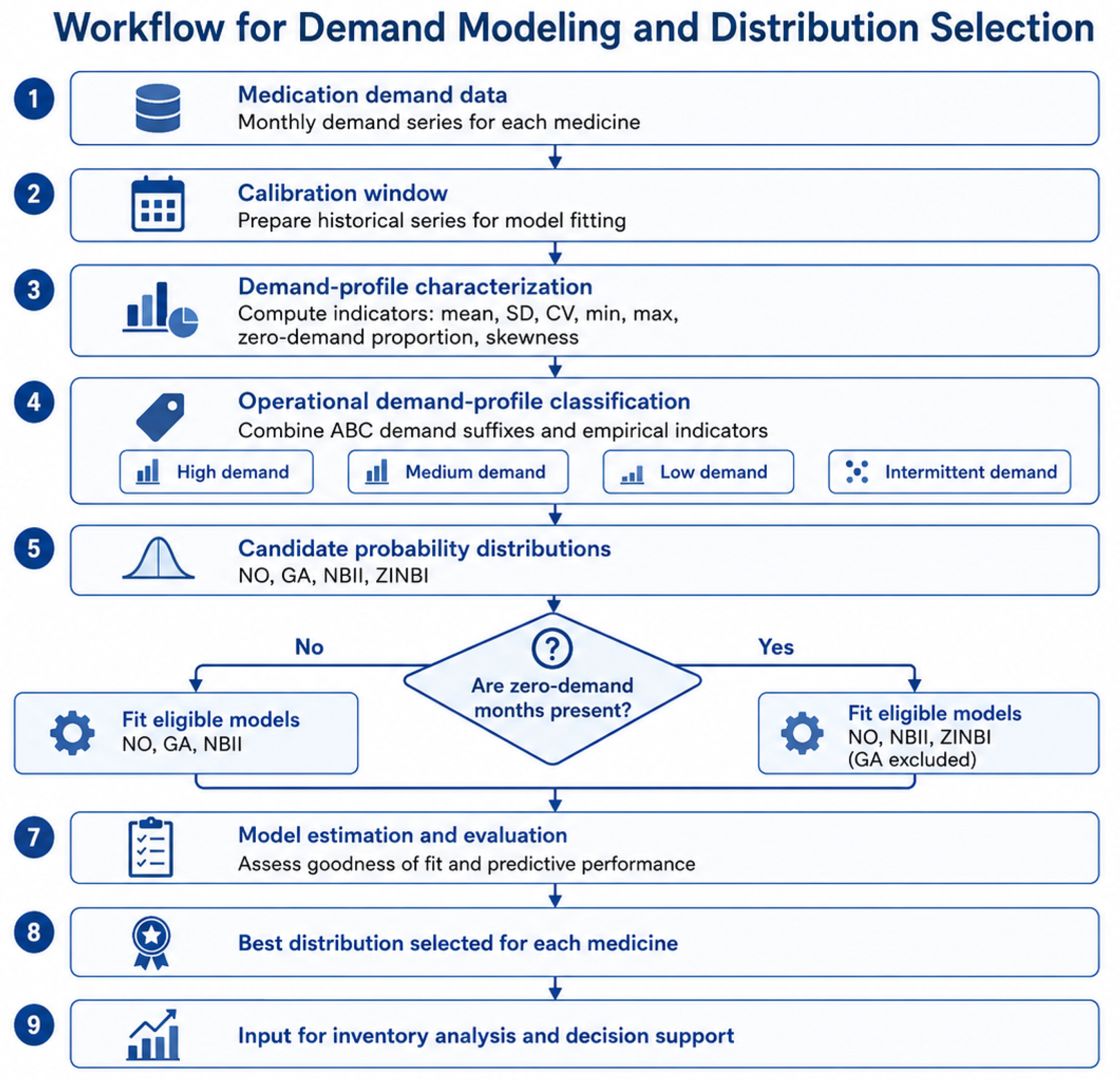
Figure 2.
Representative monthly demand profiles from the case study: (a) high-demand medicine (M01), (b) medium-demand medicine (M04), (c) low-demand medicine (M09), and (d) intermittent-demand medicine (M11). Medicine identifiers were anonymized.
Figure 2.
Representative monthly demand profiles from the case study: (a) high-demand medicine (M01), (b) medium-demand medicine (M04), (c) low-demand medicine (M09), and (d) intermittent-demand medicine (M11). Medicine identifiers were anonymized.
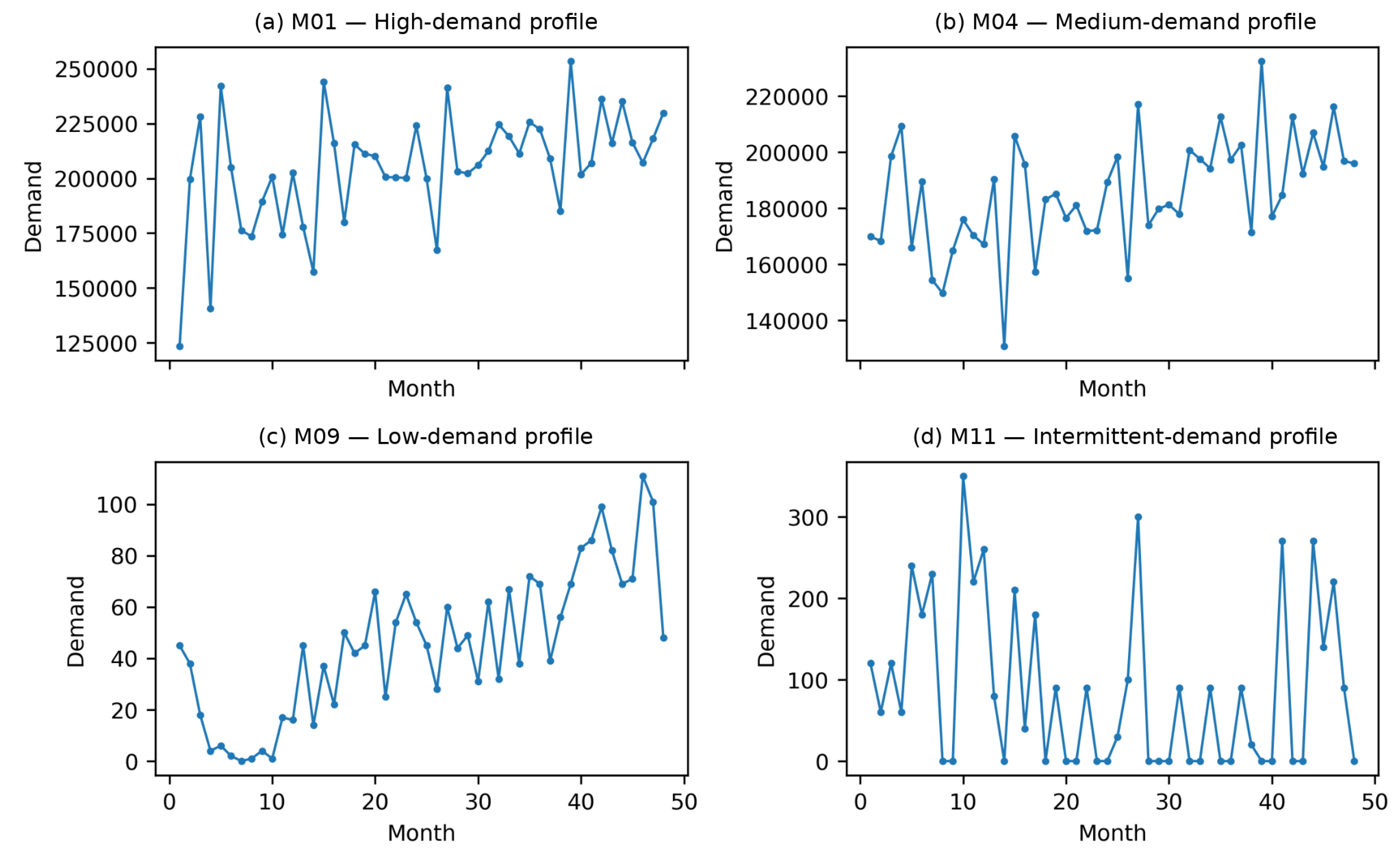
Figure 3.
Most frequent AIC-winning model in the simulation study by demand variability and zero-demand share. The heatmap shows that zero-demand frequency strongly shifts statistical model selection toward zero-inflated models.
Figure 3.
Most frequent AIC-winning model in the simulation study by demand variability and zero-demand share. The heatmap shows that zero-demand frequency strongly shifts statistical model selection toward zero-inflated models.
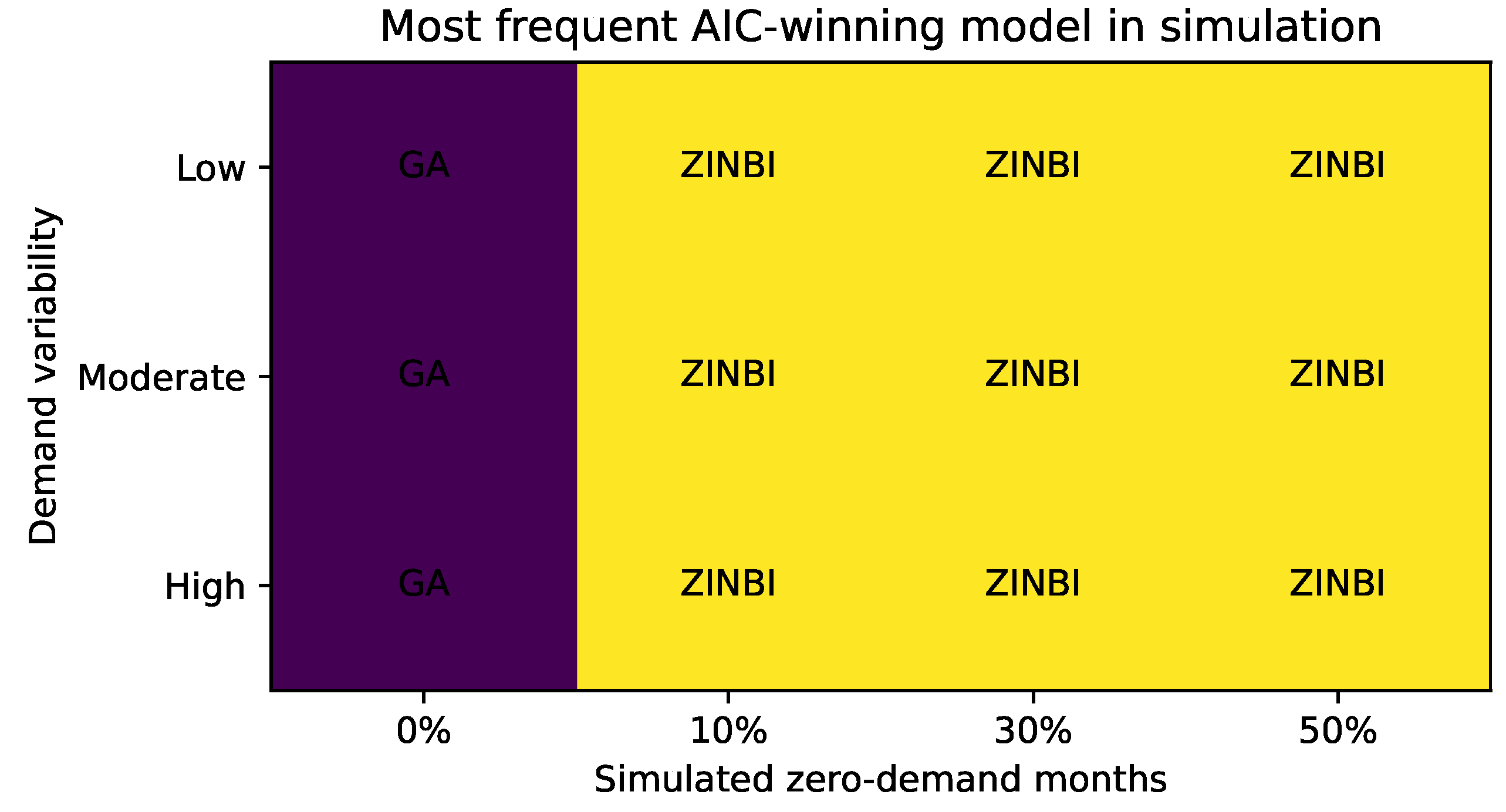
Figure 4.
Classification tree used to translate simulation outcomes into model-selection rules. The first split shows the central role of zero-demand share in distinguishing intermittent from non-intermittent demand regimes.
Figure 4.
Classification tree used to translate simulation outcomes into model-selection rules. The first split shows the central role of zero-demand share in distinguishing intermittent from non-intermittent demand regimes.
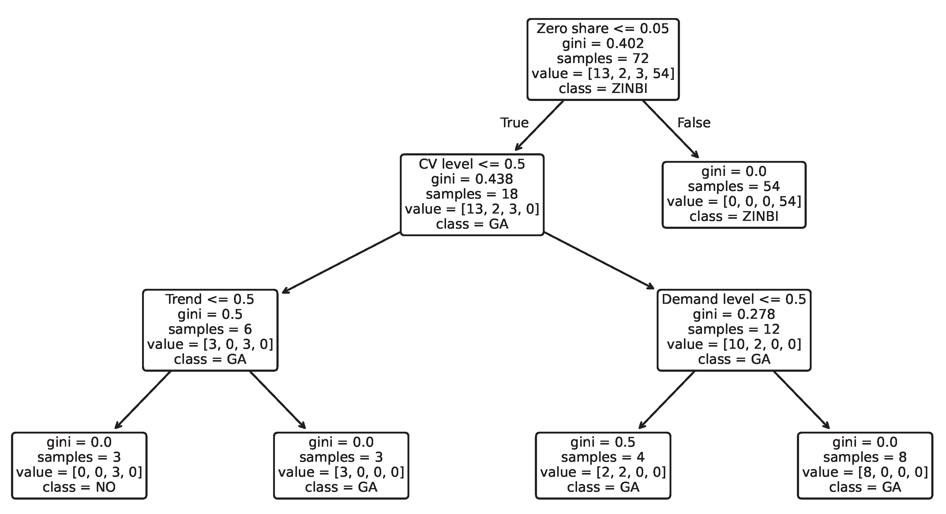

Table 1.
Positioning of the proposed demand-profile-informed inventory framework relative to related literature.
Table 1.
Positioning of the proposed demand-profile-informed inventory framework relative to related literature.
| Study | Setting or problem | Main methodological focus | Main contribution | Gap addressed by this article |
|---|---|---|---|---|
| Abu Zwaida et al. [4] | Hospital supply chain and drug shortages | Inventory optimization to prevent shortages | Highlights the need for efficient inventory policies under shortage risk | Does not provide model-selection rules by medication demand profile |
| Tucker and Daskin [6] | Pharmaceutical supply-chain reliability | Reliability modelling, disruption risk, recovery, redundancy | Links supply-chain configuration with expected drug-shortage outcomes | Focuses on supply reliability rather than pharmacy-level probabilistic demand modelling |
| Bozkir et al. [5] | Health-network drug shortages | Stocking and transshipment policies under stochastic demand | Connects pharmaceutical inventory with service-level preservation during shortages | Focuses on inventory sharing and service levels, not distributional selection for heterogeneous medication demand |
| de Assis et al. [9] | Hospital medicines and materials | Multi-criteria decision analysis for inventory classification | Shows that hospital inventory classification should consider multiple criteria beyond ABC | Classifies items, but does not compare probabilistic demand models or stochastic inventory-cost outcomes |
| Chen et al. [10] | Case outpatient pharmacy | Simulation optimization of minimum–maximum inventory levels | Demonstrates that optimized inventory settings can reduce drug inventory costs | Optimizes stock levels in a case setting, but does not derive generalizable demand-profile decision rules |
| Rojas et al. [14] | Hospital pharmacy under uncertain demand | Lot-size models, skewness/kurtosis, stochastic programming | Shows that distributional shape can affect lot-size and inventory-cost decisions | Does not explicitly combine empirical profiles, simulation scenarios, and interpretable model-selection rules |
| Pinçe et al. [18] | Intermittent-demand forecasting | Critical review of intermittent-demand methods | Shows that intermittent demand requires specialized forecasting approaches | Focuses mainly on forecasting literature, not hospital pharmacy inventory-cost evaluation |
| Rožanec and Mladenić [16] | Lumpy and intermittent demand | Two-fold modelling of occurrence and demand size | Supports separating zero-demand occurrence from positive demand size | Not specific to hospital medications and not integrated with stochastic inventory optimization |
| Sanguri et al. [19] | Intermittent demand with obsolescence risk | Forecasting under intermittent demand and inventory obsolescence | Connects intermittent demand with inventory-relevant consequences | Does not address hospital pharmacy cost structures or medication demand profiles |
| Li et al. [17] | Intermittent-demand forecasting | Feature-based forecast combinations and inventory implications | Shows that demand features can guide forecasting choices and inventory outcomes | Does not translate features into hospital pharmacy probabilistic inventory-model selection rules |
| Robert et al. [12] | Clinical pharmacy decision support | Clinical decision-support system for drug-related problems | Demonstrates the value of structured pharmacy decision support | Clinical rather than logistics-oriented decision support |
| Orsini et al. [13] | Hospital medication management | Economic evaluation of automation and digitalization | Shows the economic relevance of digital medication-management systems | Evaluates digitalization benefits, not demand-profile-based inventory modelling |
| This study | Public hospital pharmacy medication supply | Empirical demand profiling, probabilistic modelling, stochastic inventory evaluation, Monte Carlo simulation, and decision-rule extraction | Integrates real hospital data and simulation evidence to derive interpretable inventory model-selection rules | Addresses the gap between statistical demand modelling and operational inventory decision-making |
Table 2.
Consolidated empirical inputs used in the hospital pharmacy inventory analysis.
| Input category | Variables used | Role in the analysis |
|---|---|---|
| Monthly demand records | Monthly medication demand over 48 months | Used to estimate descriptive demand-profile indicators, fit candidate probability distributions, and define the calibration and evaluation periods. |
| Demand-profile indicators | Mean demand, standard deviation, coefficient of variation, zero-demand share, minimum, maximum, and skewness | Used to classify medicines into recurrent, low-volume, and intermittent demand profiles and to support model-selection rules. |
| Observed operational decision | Observed replenishment quantity in the final evaluation period | Used as the empirical baseline against which model-based replenishment decisions were compared. |
| Inventory state | Initial inventory before the evaluation period | Used to compute shortages, ending inventory, and realized one-cycle cost under both observed and model-based decisions. |
| Economic parameters | Unit acquisition cost, fixed ordering cost, unit holding cost, and shortage-cost factor | Used to translate replenishment decisions into comparable total inventory costs. |
| Replenishment bound | Operational replenishment-capacity parameter | Used to restrict model-based order quantities to a realistic decision range consistent with the historical procurement scale. |
| Shortage-cost exposure | Proportional penalty applied to the unit acquisition cost | Used in the empirical cost function and represented as a sensitivity dimension in the simulation study. |
Table 3.
Simulation factors used to evaluate the robustness of probabilistic model selection.
| Factor | Levels | Empirical calibration | Methodological rationale |
|---|---|---|---|
| Demand level | Low, medium, high | Based on the observed separation between low-, medium-, and high-volume medicines in the empirical database | Represents heterogeneous medication consumption volumes in hospital pharmacy practice. |
| Demand variability | Low, moderate, high | Based on the empirical distribution of coefficients of variation | Captures uncertainty around expected monthly consumption and affects safety-stock and shortage risk. |
| Zero-demand frequency | 0%, 10%, 30%, 50% | Selected to cover recurrent, weakly intermittent, moderately intermittent, and highly intermittent profiles | Represents the transition from continuous positive demand to sparse medication consumption. |
| Temporal trend | None, increasing, decreasing | Included to reflect observed and plausible changes in patient volume, prescribing patterns, or therapeutic substitution | Evaluates the effect of systematic demand change on model selection and replenishment performance. |
| Shortage-cost exposure | Low, moderate, high | Parameterized as proportional penalties applied to unit acquisition cost | Captures the operational and financial consequences of understocking and emergency procurement. |
Table 4.
Empirical demand profiles of the medicines included in the case study. Medicine identifiers were anonymized.
Table 4.
Empirical demand profiles of the medicines included in the case study. Medicine identifiers were anonymized.
| Medicine ID | ABC group | Mean | SD | CV | Zero months | Dec-2023 demand |
|---|---|---|---|---|---|---|
| M01 | A | 205,067 | 25,919 | 0.13 | 0 | 229,907 |
| M02 | A | 1,953 | 339.9 | 0.17 | 0 | 1,381 |
| M03 | A | 655.3 | 313.2 | 0.48 | 0 | 1,390 |
| M04 | B | 185,246 | 19,989 | 0.11 | 0 | 195,965 |
| M05 | B | 70,973 | 8,259 | 0.12 | 0 | 62,130 |
| M06 | C | 224.4 | 217.7 | 0.97 | 9 | 0 |
| M07 | C | 266.5 | 177.8 | 0.67 | 8 | 360 |
| M08 | C | 109.4 | 70.5 | 0.65 | 2 | 291 |
| M09 | C | 45.5 | 28.4 | 0.62 | 1 | 48 |
| M10 | C | 182.7 | 199.4 | 1.09 | 17 | 400 |
| M11 | C | 88.3 | 102.2 | 1.16 | 20 | 0 |
| M12 | C | 48.7 | 64.0 | 1.31 | 21 | 0 |
| M13 | C | 52.7 | 94.6 | 1.79 | 33 | 0 |
0.98 Note: Medicine IDs are anonymized and preserve the ordering used throughout the analysis.
Table 5.
Distributional fit by medicine ID using AIC on the calibration window. Lower AIC values indicate better relative fit.
Table 5.
Distributional fit by medicine ID using AIC on the calibration window. Lower AIC values indicate better relative fit.
| Medicine ID | ABC group | Normal | Gamma | NBII | ZINBI | Winner |
|---|---|---|---|---|---|---|
| M01 | A | 1,092 | 1,096 | 1,096 | 1,098 | NO |
| M02 | A | 682 | 683 | 683 | 685 | NO |
| M03 | A | 672 | 658 | 659 | 660 | GA |
| M04 | B | 1,068 | 1,069 | 1,069 | 1,071 | NO |
| M05 | B | 984 | 984 | 984 | 986 | NO |
| M06 | C | 642 | – | 616 | 557 | ZINBI |
| M07 | C | 624 | – | 686 | 552 | ZINBI |
| M08 | C | 530 | – | 537 | 516 | ZINBI |
| M09 | C | 452 | – | 466 | 456 | NO |
| M10 | C | 634 | – | 562 | 457 | ZINBI |
| M11 | C | 572 | – | 497 | 396 | ZINBI |
| M12 | C | 528 | – | 424 | 360 | ZINBI |
| M13 | C | 565 | – | 321 | 244 | ZINBI |
0.98 Note: Medicine IDs are anonymized and follow the ordering reported in Table 4. Gamma was treated as non-applicable when the calibration series contained zero-demand months. Displayed AIC values are rounded; winners were determined using the unrounded values.
Table 6.
Empirical one-cycle inventory evaluation for December 2023. Costs and savings are expressed in Chilean pesos.
Table 6.
Empirical one-cycle inventory evaluation for December 2023. Costs and savings are expressed in Chilean pesos.
| Medicine ID | ABC group | Observed Q | Observed cost | Best operational model | Model-based Q | Model-based cost | Savings | Savings (%) |
|---|---|---|---|---|---|---|---|---|
| M01 | A | 292,732 | 41,059,936 | NO | 197,764 | 34,717,239 | 6,342,696 | 15.4 |
| M02 | A | 2,596 | 22,535,789 | GA | 1,361 | 11,818,274 | 10,717,515 | 47.6 |
| M03 | A | 1,525 | 25,643,385 | NO | 215 | 28,024,379 | -2,380,994 | -9.3 |
| M04 | B | 56,169 | 2,917,206 | NO | 143,800 | 2,077,224 | 839,982 | 28.8 |
| M05 | B | 69,134 | 1,418,036 | NBII | 38,462 | 580,076 | 837,960 | 59.1 |
| M06 | C | 489 | 320,987 | NO | 0 | 2,148 | 318,839 | 99.3 |
| M07 | C | 219 | 98,400 | NO | 0 | 4,296 | 94,104 | 95.6 |
| M08 | C | 117 | 35,656 | NO | 0 | 4,009 | 31,648 | 88.8 |
| M09 | C | 84 | 1,246,795 | NO | 15 | 404,218 | 842,577 | 67.6 |
| M10 | C | 243 | 570,364 | NO | 0 | 294,615 | 275,750 | 48.3 |
| M11 | C | 48 | 41,096 | NO | 0 | 2,864 | 38,232 | 93.0 |
| M12 | C | 41 | 26,907 | NO | 0 | 2,134 | 24,773 | 92.1 |
| M13 | C | 0 | 2,434 | NO | 0 | 2,434 | 0 | 0.0 |
Table 7.
Distribution-specific first-stage decisions and realized inventory-cost outcomes in the empirical case. Costs are expressed in Chilean pesos. Gamma was treated as non-applicable when the calibration series contained zero-demand months.
Table 7.
Distribution-specific first-stage decisions and realized inventory-cost outcomes in the empirical case. Costs are expressed in Chilean pesos. Gamma was treated as non-applicable when the calibration series contained zero-demand months.
| Medicine ID | Group | Distribution | Realized shortage | Realized overstock | Realized cost | ||
|---|---|---|---|---|---|---|---|
| M01 | A | NO | 197,764 | 1 | 29,656 | 0 | 34,717,239 |
| M01 | A | GA | 196,499 | 1 | 30,921 | 0 | 34,868,257 |
| M01 | A | NBII | 196,834 | 1 | 30,586 | 0 | 34,828,264 |
| M01 | A | ZINBI | 197,142 | 1 | 30,278 | 0 | 34,791,495 |
| M02 | A | NO | 1,392 | 1 | 0 | 563 | 12,087,271 |
| M02 | A | GA | 1,361 | 1 | 0 | 532 | 11,818,274 |
| M02 | A | NBII | 1,362 | 1 | 0 | 533 | 11,826,951 |
| M02 | A | ZINBI | 1,371 | 1 | 0 | 542 | 11,905,047 |
| M03 | A | NO | 215 | 1 | 776 | 0 | 28,024,379 |
| M03 | A | GA | 185 | 1 | 806 | 0 | 28,463,486 |
| M03 | A | NBII | 174 | 1 | 817 | 0 | 28,624,492 |
| M03 | A | ZINBI | 181 | 1 | 810 | 0 | 28,522,033 |
| M04 | B | NO | 143,800 | 1 | 23,080 | 0 | 2,077,224 |
| M04 | B | GA | 143,378 | 1 | 23,502 | 0 | 2,081,269 |
| M04 | B | NBII | 143,721 | 1 | 23,159 | 0 | 2,077,981 |
| M04 | B | ZINBI | 143,518 | 1 | 23,362 | 0 | 2,079,927 |
| M05 | B | NO | 38,617 | 1 | 0 | 4,328 | 584,311 |
| M05 | B | GA | 38,733 | 1 | 0 | 4,444 | 587,480 |
| M05 | B | NBII | 38,462 | 1 | 0 | 4,173 | 580,076 |
| M05 | B | ZINBI | 38,584 | 1 | 0 | 4,295 | 583,409 |
| M06 | C | NO | 0 | 0 | 0 | 150 | 2,148 |
| M06 | C | GA | – | – | – | – | – |
| M06 | C | NBII | 0 | 0 | 0 | 150 | 2,148 |
| M06 | C | ZINBI | 0 | 0 | 0 | 150 | 2,148 |
| M07 | C | NO | 0 | 0 | 0 | 300 | 4,296 |
| M07 | C | GA | – | – | – | – | – |
| M07 | C | NBII | 0 | 0 | 0 | 300 | 4,296 |
| M07 | C | ZINBI | 0 | 0 | 0 | 300 | 4,296 |
| M08 | C | NO | 0 | 0 | 18 | 0 | 4,009 |
| M08 | C | GA | – | – | – | – | – |
| M08 | C | NBII | 0 | 0 | 18 | 0 | 4,009 |
| M08 | C | ZINBI | 0 | 0 | 18 | 0 | 4,009 |
| M09 | C | NO | 15 | 1 | 6 | 0 | 404,218 |
| M09 | C | GA | – | – | – | – | – |
| M09 | C | NBII | 11 | 1 | 10 | 0 | 455,236 |
| M09 | C | ZINBI | 0 | 0 | 21 | 0 | 575,225 |
| M10 | C | NO | 0 | 0 | 70 | 0 | 294,615 |
| M10 | C | GA | – | – | – | – | – |
| M10 | C | NBII | 0 | 0 | 70 | 0 | 294,615 |
| M10 | C | ZINBI | 0 | 0 | 70 | 0 | 294,615 |
| M11 | C | NO | 0 | 0 | 0 | 200 | 2,864 |
| M11 | C | GA | – | – | – | – | – |
| M11 | C | NBII | 0 | 0 | 0 | 200 | 2,864 |
| M11 | C | ZINBI | 0 | 0 | 0 | 200 | 2,864 |
| M12 | C | NO | 0 | 0 | 0 | 149 | 2,134 |
| M12 | C | GA | – | – | – | – | – |
| M12 | C | NBII | 0 | 0 | 0 | 149 | 2,134 |
| M12 | C | ZINBI | 0 | 0 | 0 | 149 | 2,134 |
| M13 | C | NO | 0 | 0 | 0 | 170 | 2,434 |
| M13 | C | GA | – | – | – | – | – |
| M13 | C | NBII | 0 | 0 | 0 | 170 | 2,434 |
| M13 | C | ZINBI | 0 | 0 | 0 | 170 | 2,434 |
Table 8.
Simulation summary: most frequent AIC-winning model across demand levels and trend scenarios.
Table 8.
Simulation summary: most frequent AIC-winning model across demand levels and trend scenarios.
| Variability | 0% zeros | 10% zeros | 30% zeros | 50% zeros |
|---|---|---|---|---|
| Low | GA | ZINBI | ZINBI | ZINBI |
| Moderate | GA | ZINBI | ZINBI | ZINBI |
| High | GA | ZINBI | ZINBI | ZINBI |
Table 9.
Practical decision rules derived from the empirical and simulation analyses.
| Demand condition | Recommended model | Rationale |
|---|---|---|
| High or medium demand with low-to-moderate zeros | Normal or NBII | Stable demand can often be captured by lower-complexity models, while NBII accommodates count dispersion. |
| Low demand with positive skew and no structural zeros | Gamma or NBII | Asymmetry and non-negative support become more relevant as volume decreases. |
| Intermittent demand with repeated zero months | ZINBI | Explicit zero inflation avoids forcing all zeros through the count component. |
| High shortage-cost or tight budget scenarios | Compare candidates by inventory cost, not AIC alone | The statistically best fit is not always the economically best decision. |
Disclaimer/Publisher’s Note: The statements, opinions and data contained in all publications are solely those of the individual author(s) and contributor(s) and not of MDPI and/or the editor(s). MDPI and/or the editor(s) disclaim responsibility for any injury to people or property resulting from any ideas, methods, instructions or products referred to in the content. |
© 2026 by the authors. Licensee MDPI, Basel, Switzerland. This article is an open access article distributed under the terms and conditions of the Creative Commons Attribution (CC BY) license (http://creativecommons.org/licenses/by/4.0/).
Copyright: This open access article is published under a Creative Commons CC BY 4.0 license, which permit the free download, distribution, and reuse, provided that the author and preprint are cited in any reuse.


